AWS Big Data Blog: Recent Episodes
None

It’s AWS re:Invent time, where you turn your ideas into reality. Get a front row seat to hear real stories from AWS customers, experts and leaders about navigating pressing topics like generative AI and data analytics.
For data enthusiasts and data professionals alike, this blog is a curated and comprehensive guide to all analytics sessions, for you to efficiently plan your itinerary. Secure your spot early for must-attend sessions through the attendee portal. Can’t join in person? No worries – grab a free pass to stream live sessions online.
Join us at the AWS Analytics Kiosk in the AWS Village Expo to get your data questions answered by AWS experts, to dive deeper into re:Invent launches, participate in a data-centric quiz and AWS authored book giveaways.
Keynotes KEY002 | CEO Keynote with Matt Garman | Tuesday, Dec 3 | 8:00 AM – 10:30 AM PST | Venetian | Level 2 | Venetian Ballroom F
Join AWS CEO Matt Garman to hear how AWS is innovating across every aspect of the world’s leading cloud. He explores how we are reinventing foundational building blocks as well as developing brand new experiences, all to empower customers and partners with what they need to build a better future.
KEY003 | Swami Sivasubramanian, Vice President, Data and AI at AWS | Wednesday, Dec 4 | 8:00 AM – 10:30 AM PST | Venetian | Level 2 | Venetian Ballroom F
Join Dr. Swami Sivasubramanian, VP of AI and Data at AWS, to discover how you can use a strong data foundation to create innovative and differentiated solutions for your customers. Hear from customer speakers with real-world examples of how they’ve used data to support a variety of use cases, including generative AI, to create unique customer experiences.
KEY005 | Dr. Werner Vogels (Vice President and Chief Technology Officer, Amazon.com) | Thursday, Dec 5 | 8:30 AM – 10:30 AM PST | Venetian | Level 2 | Venetian Ballroom F
Join Dr. Werner Vogels, VP and CTO at Amazon.com, as he shares the critical lessons and strategies he’s learned for managing increasingly complex systems. The keynote explores the core principles for embracing complexity, drawing on Amazon experiences building distributed systems at massive scale.
Analytics Innovation Talk ANT204-INT | Beyond boundaries: Converging analytics and AI to reshape the future | Wednesday, Dec 4 | 2:30 PM – 3:30 PM PST | Venetian | Level 5 | Palazzo Ballroom B
The boundaries between data analytics and AI are blurring as data workers’ behaviors evolve, and previously distinct data roles and use cases converge. Getting to near real-time, trustworthy insights has become paramount, so data workers are seeking seamless collaboration and interoperability across tools and data sources. In this talk, join Sirish Chandrasekaran, Director for Data Warehousing at AWS, and Rick Sears, Director for Data Processing at AWS, to envision a future with AWS where your data workers can effortlessly move between analyzing historical patterns, predicting future scenarios, and automating decision flows at scale, breaking through disparate tools and siloed workflows.
Breakout sessions Dive into cutting-edge topics with re:Invent breakout sessions. These immersive, hour-long lectures are led by AWS experts, customers, and partners, offering you unparalleled insights and knowledge in a concise format. Whether you’re exploring the latest in cloud technology, AWS Analytics advancements, or industry-specific solutions, these sessions are designed to expand your horizon and inspire your next big idea.
| Monday, Dec 2 | Tuesday, Dec 3 | Wednesday, Dec 4 | Thursday, Dec 5 | | 8:30 AM – 9:30 AM PST | MGM Grand ANT324 | Accelerate value from data: Migrating from batch to stream processing | 12:00 PM – 1:00 PM PST | Caesars Forum ANT341 | Enhance performance with observability, security, and log analytics | 8:30 AM – 9:30 AM PST | Mandalay Bay ANT343 | Monitor and manage data quality | 11:00 AM – 12:00 PM PST |Mandalay Bay ANT325 | Achieve seamless and secure data sharing | | 10:00 AM – 11:00 AM PST| Mandalay Bay ANT335 | Build highly performant data solutions with serverless analytics | 12:00 PM – 1:00 PM PST | MGM Grand ANT327 | What’s new: Data streaming on AWS | 9:00 AM – 10:00 AM PST | MGM Grand BSI201|Supercharge your apps with embedded Amazon QuickSight and Amazon Q | 11:00 AM – 12:00 PM PST | MGM Grand ANT340 | Revolutionize your search applications for generative AI | | 1:00 PM – 2:00 PM PST | Mandalay Bay ANT342 | Operate and scale managed Apache Kafka and Apache Flink clusters | 1:30 PM – 2:30 PM PST | MGM Grand ANT349| Innovations in AWS analytics: Data warehousing and SQL analytics | 10:00 AM – 11:00 AM PST | Mandalay Bay ANT336 | Build large-scale transactional data lakes with open table formats | 11:30 AM – 12:30 PM PST | Caesars Forum ANT344 | Cost-effective data processing with Amazon EMR | | 1:00 PM – 2:00 PM PST | Wynn BSI101 | Reimagine business intelligence with generative AI | 1:30 PM – 2:30 PM PST | Wynn ANT334 | Scale with self-service analytics on AWS | 11:30 AM – 12:30 PM PST | Mandalay Bay ANT329 | What’s new in search, observability & vectors in Amazon OpenSearch Service | . | | 5:30 PM – 6:30 PM PST | Mandalay Bay ANT347 | Maximize efficiency and reduce costs with Amazon OpenSearch Service | 2:30 PM – 3:30 PM PST | Mandalay Bay ANT328 | AI-powered analytics with Amazon Redshift Serverless & data sharing | 11:30 AM – 12:30 PM PST | Mandalay Bay BSI102 | What’s new with Amazon QuickSight | . | | . | 3:00 PM – 4:00 PM PST | Caesars Forum ANT346 | Innovations in AWS analytics: Data processing | 12:00 PM – 1:00 PM PST| Mandalay Bay ANT339 | Scaling to new heights with Amazon Redshift multi-cluster architecture | . | | . | 4:00 PM – 5:00 PM PST | Venetian ANT302 | Data foundation in the age of generative AI | 1:00 PM – 2:00 PM PST | Mandalay Bay ANT303 | Explore what’s new in data governance with AWS analytics | . | | . | 4:00 PM – 5:00 PM PST | Mandalay Bay ANT202 | Demystify and democratize access to your data with a business catalog | 1:00 PM – 2:00 PM PST | Mandalay Bay ANT330 | Solving different data ingestion use cases with AWS | . | | . | 4:00 PM – 5:00 PM PST | Wynn ANT348 | Innovations in AWS analytics: Zero-ETL and data integrations | . | . | | . | 4:00 PM – 5:00 PM PST | Mandalay Bay BSI206 | Scale BI to all your users with Amazon Q in QuickSight | . | . | | . | 5:30 PM – 6:30 PM PST | MGM Grand BSI205 | Migrate to QuickSight: Reduce costs and increase productivity | . | . | | . | 5:30 PM – 6:30 PM PST | MGM Grand ANT345 | Modernize your data warehouse by moving to Amazon Redshift | . | . |
Chalk talks These hour-long, highly engaging sessions offer a unique blend of expert insight and collaborative learning. An AWS specialist kicks off with a concise, informative lecture, setting the stage for an in-depth, interactive Q&A. With a limited audience size, you’ll have the opportunity to dive deep into topics, ask pressing questions, and engage in meaningful discussions with both the presenter and fellow attendees.
| Monday, Dec 2 | Tuesday, Dec 3 | Wednesday, Dec 4 | Thursday, Dec 5 | | 10:00 AM – 11:00 AM PST | MGM Grand ANT316-R | Architectural patterns for near real-time data analytics on AWS | 11:30 AM – 12:30 PM PST | Caesars Forum ANT315 | Amazon OpenSearch Service cost optimizations | 10:00 AM – 11:00 AM PST | Mandalay Bay ANT305 | Strategies for efficient zero-ETL integrations | 11:00 AM – 12:00 PM PST | Mandalay Bay ANT304-R1 | Accelerating the shift from batch to stream processing | | 11:30 AM – 12:30 PM PST | MGM Grand ANT337-R | Cost optimization for data analytics on AWS | 11:30 AM – 12:30 PM PST | Wynn ANT410 | Maximize your data performance with Amazon EMR on Amazon EKS | 10:30 AM – 11:30 AM PST | MGM Grand BSI304 | Security and governance: Safeguarding your data with Amazon QuickSight | 12:30 PM – 1:30 PM PST | Mandalay Bay ANT411 | Data integration with AWS Glue and Amazon MWAA | | 11:30 AM – 12:30 PM PST | MGM Grand ANT337-R | Cost optimization for data analytics on AWS | 12:00 PM – 1:00 PM PST | MGM Grand ANT332-R | Democratize generative AI data access without compromising on security | 11:30 AM – 12:30 PM PST | Mandalay Bay ANT331-R1 | Build your data strategy for generative AI with Amazon Redshift | 12:30 PM – 1:30 PM PST | MGM Grand ANT409-R1 | Optimize Apache Spark workloads with Amazon EMR Serverless | | 1:00 PM – 2:00 PM PST | Mandalay Bay ANT318 | Build serverless streaming data pipelines for real-time analytics | 1:00 PM – 2:00 PM PST | MGM Grand ANT326 | Build multi-tenant data processing architectures | 1:00 PM – 2:00 PM PST | Wynn ANT317-R1 | Best practices for migrating to Amazon OpenSearch Service | 2:00 PM – 3:00 PM PST | Mandalay Bay ANT320 | Data preparation authoring with AWS Glue Studio | | 2:30 PM – 3:30 PM PST | Mandalay Bay ANT412 | Ingest streaming data into Apache Iceberg tables with AWS streaming | 1:00 PM – 2:00 PM PST | Caesars Forum ANT413-R | Data governance with AWS analytics | 1:00 PM – 2:00 PM PST | Caesars Forum ANT323-R1 | Catalog and govern your data for generative AI | 2:00 PM – 3:00 PM PST | MGM Grand ANT338 | Using natural language to author data integration applications | | 4:00 PM – 5:00 PM PST | Caesars Forum ANT317-R | Best practices for migrating to Amazon OpenSearch Service | 1:30 PM – 2:30 PM PST | Wynn ANT323-R | Catalog and govern your data for generative AI | 1:00 PM – 2:00 PM PST | Mandalay Bay ANT414-R1 | Scalable design patterns for Apache Iceberg–based data lakes | 3:30 PM – 4:30 PM PST | MGM Grand ANT413-R1 | Data governance with AWS analytics | | 5:30 PM – 6:30 PM PST | Caesars Forum ANT304-R | Accelerating the shift from batch to stream processing | 2:30 PM – 3:30 PM PST | Wynn ANT314 | Add search to your existing databases with Amazon OpenSearch Ingestion | 2:30 PM – 3:30 PM PST | Caesars Forum ANT333 | Streamline data access management with trusted identity propagation | . | | . | 2:30 PM – 3:30 PM PST | Caesars Forum ANT331-R | Build your data strategy for generative AI with Amazon Redshift | 4:00 PM – 5:00 PM PST | Caesars Forum ANT321 | Model your business structure with Amazon DataZone | . | | . | 3:00 PM – 4:00 PM PST | MGM Grand ANT319 | Create a data marketplace with Amazon DataZone | 4:00 PM – 5:00 PM PST | MGM Grand ANT322 | Modernize and simplify ETL with AWS Glue | | . | 4:00 PM – 5:00 PM PST | Caesars Forum ANT414-R | Scalable design patterns for Apache Iceberg–based data lakes | 4:30 PM – 5:30 PM PST | Caesars Forum ANT337-R1 | Cost optimization for data analytics on AWS | . | | . | 4:30 PM – 5:30 PM PST | MGM Grand ANT409-R | Optimize Apache Spark workloads with Amazon EMR Serverless | 5:30 PM – 6:30 PM PST | MGM Grand ANT332-R1 | Democratize generative AI data access without compromising on security | . | | . | 5:30 PM – 6:30 PM PST | Caesars Forum ANT316-R1 | Architectural patterns for near real-time data analytics on AWS | . | . |
Builders’ sessions Immerse yourself in our builders’ sessions – a hands-on learning experience designed to elevate your AWS skills. These focused, hour-long workshops bring together a small group of up to ten attendees with a dedicated AWS expert at each table.
| Monday, Dec 2 | Tuesday, Dec 3 | Wednesday, Dec 4 | | 8:30 AM – 9:30 AM PST | Caesars Forum ANT306-R | Orchestrate data and ML workflows with managed Apache Airflow | 12:00 PM – 1:00 PM PST | Caesars Forum ANT307-R | Seamless data sharing with Amazon Redshift | 8:30 AM – 9:30 AM PST | Caesars Forum ANT307-R3 | Seamless data sharing with Amazon Redshift | | 5:30 PM – 6:30 PM PST | Caesars Forum ANT306-R1 | Orchestrate data and ML workflows with managed Apache Airflow | 12:00 PM – 1:00 PM PST | Wynn ANT401 | Vector search with Amazon OpenSearch Service | . | | . | 1:30 PM – 2:30 PM PST | Wynn ANT306-R2 | Orchestrate data and ML workflows with managed Apache Airflow | . | | . | 1:30 PM – 2:30 PM PST | Caesars Forum ANT307-R1 | Seamless data sharing with Amazon Redshift | . | | . | 3:00 PM – 4:00 PM PST | Caesars Forum ANT307-R2 | Seamless data sharing with Amazon Redshift | . | | . | 4:30 PM – 5:30 PM PST | Caesars Forum ANT306-R3 | Orchestrate data and ML workflows with managed Apache Airflow | . |
Workshops Roll your sleeves in our dynamic 2-hour workshops, where you’ll tackle real-world challenges using AWS services. These interactive sessions kick off with a brief, informative lecture to set the stage, then quickly transition into hands-on problem-solving. Bring your laptop and prepare to build alongside AWS experts, who will guide you through practical applications of cloud computing concepts. Whether you’re new to AWS or looking to sharpen your skills, these workshops offer a unique opportunity to learn by doing, enabling you to leave with confidence and applicable knowledge in AWS technologies.
| Mon, Dec 2 | Tuesday, Dec 3 | Wednesday, Dec 4 | Thursday, Dec 5 | | 12:00 PM – 2:00 PM PST | Mandalay Bay ANT404 | Migrating from self-managed Apache Kafka to Amazon MSK | 11:30 AM – 1:30 PM PST | Venetian ANT309 | Enhance insights for your data warehouse with zero-ETL & generative AI | 9:00 AM – 11:00 AM PST | MGM Grand ANT310 | Low-cost logging and observability with Amazon OpenSearch Service | 12:00 PM – 2:00 PM PST | Mandalay Bay ANT350-R1 | End-to-end data integration and data engineering on AWS | | 3:00 PM – 5:00 PM PST | Mandalay Bay ANT312 | Unlock your enterprise data with intelligent document search | 11:30 AM – 1:30 PM PST | MGM Grand BSI204-R | Hands-on with Amazon Q in QuickSight: A step-by-step workshop | 1:00 PM – 3:00 PM PST | MGM Grand ANT350-R | End-to-end data integration and data engineering on AWS | 3:00 PM – 5:00 PM PST | Mandalay Bay ANT402-R1 | Build open table data lakes for real-time insights with Apache Iceberg | | . | 12:30 PM – 2:30 PM PST | Caesars Forum ANT402-R | Build open table data lakes for real-time insights with Apache Iceberg | 4:00 PM – 6:00 PM PST | MGM Grand ANT308-R1 | Build and govern your data mesh with Amazon DataZone | 3:30 PM – 5:30 PM PST | Venetian BSI204-R1 | Hands-on with Amazon Q in QuickSight: A step-by-step workshop | | . | 3:30 PM – 5:30 PM PST | Wynn ANT308-R | Build and govern your data mesh with Amazon DataZone | . | . | | . | 4:30 PM – 6:30 PM PST | MGM Grand ANT311 | Prepare your data for generative AI | . | . |
Code talks Dive into the world of practical AWS development with our engaging Code Talks. These sessions elevate the popular chalk talk format by shifting focus from architectural concepts to hands-on coding. Watch as expert speakers guide you through live coding demonstrations, showcasing real-world solutions in action. You’ll gain insights into the reasoning behind each implementation choice and witness the development process unfold in real-time. Whether you’re a seasoned developer or just starting your AWS journey, Code Talks offer a unique opportunity to enhance your skills and deepen your understanding of AWS solutions through practical, code-centric discussions.
| Mon, Dec 2 | Tuesday, Dec 3 | Wednesday, Dec 4 | Thursday, Dec 5 | | 1:00 PM – 2:00 PM PST | Wynn ANT407 | Predictive maintenance with Amazon Managed Service for Apache Flink | 3:00 PM – 4:00 PM PST | Wynn ANT406-R | Generative AI–powered search with Amazon OpenSearch Service | 12:00 PM – 1:00 PM PST | Wynn ANT408 | Working with UDFs in Amazon Redshift and Amazon Athena | 2:30 PM – 3:30 PM PST | Wynn ANT406-R1 | Generative AI–powered search with Amazon OpenSearch Service |
Session IDs for chalk talks, builders’ sessions, workshops, and code talks that end with R (for example, ANT406-R), indicate repeat sessions.
Conclusion We hope this post acts as your go-to resource for navigating the AWS analytics track at re:Invent 2024. For staying in the know about the most recent trends and advancements in AWS Analytics, follow our LinkedIn page.
About the Authors Imtiaz (Taz) Sayed is the WW Tech Leader for Analytics at AWS. He enjoys engaging with the community on all things data and analytics. He can be reached through LinkedIn.
Navnit Shukla serves as an AWS Specialist Solutions Architect with a focus on Analytics. He possesses a strong enthusiasm for assisting clients in discovering valuable insights from their data. Through his expertise, he constructs innovative solutions that empower businesses to arrive at informed, data-driven choices. Notably, Navnit Shukla is the accomplished author of the book titled Data Wrangling on AWS. He can be reached through LinkedIn.
Many organizations specializing in communications and navigation surveillance technologies are required to support multi-modal transportation supply chain markets such as road, water, air, space, and rail. One common use case is provisioning of emergency alerts services for multiple government agencies.
These organizations use third-party satellite-powered terminal devices for remote monitoring using telemetry and NMEA-0183 formatted messages generated in near real time. This post demonstrates how to implement a satellite-based remote alerting and response solution on the AWS Cloud to provide time-critical alerts and actionable insights, with a focus on telemetry message ingestion and alerts. Key services in the solution include Amazon API Gateway, Amazon Data Firehose, and Amazon Location Service.
The challenge In the event of a disaster e.g. water flood, there is usually a lack of terrestrial data connectivity that prevents monitoring stations from taking actionable measures in real time. In the space analytics domain, many organizations deploy satellite-powered terminals on these monitoring stations.
These terminal devices transmit telemetry and NMEA-0183 formatted messages to a satellite network managed by a third-party entity, which is subsequently traversed down to an API endpoint.
Our AWS-powered solution aims to capture, enrich, and ingest satellite-powered telemetry messages as well as deliver alerts in near real time. This solution is based on AWS serverless services such as API Gateway, Data Firehose, and Amazon Simple Storage Service (Amazon S3), and is able to scale to more than a million terminal devices transmitting an hourly state of health telemetry message over the satellite.
Solution overview This telemetry message processing begins with an API endpoint created using API Gateway, securing HTTPS transmission over a satellite network. This endpoint receives raw JSON messages and responds with an HTTP 200 success code. We take advantage of the direct integration between API Gateway and Data Firehose to ingest these messages into Amazon S3 in near real time. The default message reception limit on an API Gateway endpoint is 10,000 messages per second, which can be increased upon request.
Upon receiving messages through API Gateway, Data Firehose batches them into 60-second intervals or 1 MB size files, whichever comes first, and delivers them to Amazon S3. This configuration enables near real-time processing, which is essential for timely alerts and responses. We use the built-in features of Data Firehose, including AWS Lambda for necessary data transformation and Amazon Simple Notification Service (Amazon SNS) for near real-time alerts. Additionally, Data Firehose converts JSON data to Parquet format before delivering it to Amazon S3, optimizing data consumption by tools like Amazon Athena, which are ideal for partitioned data formats.
To maintain up-to-date data, an AWS Glue crawler reads and updates the AWS Glue Data Catalog from transformed Parquet files. This crawler runs one time a day by default to optimize costs, but you can adjust its schedule to meet varying end-user requirements.
We use an AWS CloudFormation template to implement the solution architecture, as illustrated in the following diagram.
Cloudformation template to implement the solution architecture
For this post, we deliver sample JSON formatted telemetry messages to an API Gateway endpoint test interface to simulate the satellite-powered terminal device functionality. API Gateway integrates with Data Firehose, which uses Lambda to perform the following actions in near real time:
- Parse the message and decode the data blob from base64 encoding to utf-8. Most third-party satellite-powered terminal devices transmit messages in an encoded format and require decoding to a standard readable format such as utf-8.
- Use Amazon Location and append with location specifics (such as street, city, and ZIP) based on the latitude and longitude of the terminal device.
- Detect if the solar panel battery of the terminal device is lower than the defined threshold and generate an alert through Amazon SNS to the user-provided email address. For simplicity, the CloudFormation template creates an SNS topic within the same account instead of a cross-account consumer application. You must subscribe to the topic using an email received at the provided email address.
- Ingest the messages in an S3 bucket received in 1 minute or aggregate to 1 MB size files.
The solution uses the following key services:
- Amazon API Gateway – API Gateway is a fully managed service that makes it straightforward developers to create, publish, maintain, monitor, and secure APIs at any scale. APIs act as the entry point for applications to access data, business logic, or functionality from your backend services.
- Amazon Data Firehose – Data Firehose is an extract, transform, and load (ETL) service that reliably captures, transforms, and delivers streaming data to data lakes, data stores, and analytics services.
- AWS Glue – The AWS Glue Data Catalog is your persistent technical metadata store in the AWS Cloud. Each AWS account has one Data Catalog per AWS Region. Each Data Catalog is a highly scalable collection of tables organized into databases. A table is metadata representation of a collection of structured or semi-structured data stored in sources such as Amazon Relational Database Service (Amazon RDS), Apache Hadoop Distributed File System (HDFS), Amazon OpenSearch Service, and others.
- IAM – With AWS Identity and Access Management (IAM), you can specify who or what can access services and resources in AWS, centrally manage fine-grained permissions, and analyze access to refine permissions across AWS.
- AWS Lambda – Lambda is a serverless, event-driven compute service that lets you run code for virtually any type of application or backend service without provisioning or managing servers. You can invoke Lambda functions from over 200 AWS services and software as a service (SaaS) applications, and only pay for what you use.
- Amazon Location Service – Location Service makes it straightforward for developers to add location functionality, such as maps, points of interest, geocoding, routing, tracking, and geofencing, to their applications without sacrificing data security and user privacy.
- Amazon S3 – Amazon S3 is an object storage service offering industry-leading scalability, data availability, security, and performance. Customers of all sizes and industries can store and protect any amount of data for virtually any use case, such as data lakes, cloud-centered applications, and mobile apps.
- Amazon SNS – Amazon SNS sends notifications two ways: application-to-application (A2A) and application-to-person (A2P). A2A provides high-throughput, push-based, many-to-many messaging between distributed systems, microservices, and event-driven serverless applications. These applications include Amazon Simple Queue Service (SQS), Data Firehose, Lambda, and other HTTPS endpoints. A2P functionality lets you send messages to your customers with SMS texts, push notifications, and email.
Deploy the solution AWS CloudFormation creates the API Gateway endpoint, Data Firehose delivery stream, Lambda function, Amazon Location index, SNS topic, S3 bucket, and AWS Glue database, table, and crawler. To deploy the solution, launch the CloudFormation stack and provide the following parameters:
- S3 bucket name – The bucket that stores terminal device messages ingested in near real time by the Data Firehose delivery stream
- Email address – The email of the user to subscribe for SNS alerts
- Database name – The name of the AWS Glue database
Test the solution The following is a sample JSON state of health telemetry message transmitted by a terminal device:
{ "packetId": 29957891, "deviceType": 1, "deviceId": 6113, "userApplicationId": 65535, "organizationId": 65681, "data": "eyJsbiI6LTEwNC45NTUsInNpIjowLjAsImJpIjowLjIxMiwic3YiOjAuMDA4LCJsdCI6MzkuNTc1MiwiYnYiOjMuNzI4LCJkIjoxNjU4NzQ1MzM2LCJuIjo2NjksImEiOjE3MzguMCwicyI6NS4wLCJjIjozMjAuMCwiciI6LTEwMSwidGkiOjAuMDM2fQ==", "len": 142, "status": 0, "hiveRxTime": "2022-07-25T13:03:29"}
The data blob in the preceding sample telemetry message is encoded in base64. The following chart explains the metadata of each key indicating state of health and location of the terminal device.
| Parameter | Key | Sample Value | Notes | | Longitude | ln | -104.955 | Negative = Westing from PM | | Solar Panel Current | si | 0.176 | (Amps) | | Battery Current | bi | 0.228 | (Amps) | | Solar Panel Voltage | sv | 19.088 | (Volts) | | Latitude | lt | 39.5751 | Positive = Northing from Equator | | Battery Voltage | bv | 4.12 | (Volts) Full charge ~4.12V Dead ~ 3.3V | | Date and Time | d | 1658248415 | Epoch Seconds | | Number of Messages Sent Since Last Power Cycle | n | 531 | | Altitude | a | 1721.0 | (Meters) GPS value | | Speed | s | 1.0 | (km/h) Stationary terminal reports non-zero value | | Course: | c | 139.0 | (degrees) Nautical heading convention | | Last RSSI Value | r | -100 | (dBm) >-90 = marginal link. | | Modem Current | ti | 0.04 | (Amps) |
These telemetry messages can vary based on the default configuration of the device terminal manufacturer or user definitions.
To demonstrate the capability of the solution, we send the sample telemetry message to the API Gateway endpoint through its test interface, as shown in the following screenshot.
Sending sample telemetry message
After about a minute, you should see the delivered message to Amazon S3 through Data Firehose in the stage folder.
Delivered message to Amazon S3
You should also receive an SNS alert at the provided email address.
SNS alert message
To see the results in Athena, we crawl this data with the AWS Glue crawler created by the CloudFormation template. By default, the crawler is scheduled daily to reflect newer records for the day in the stage table.
AWS Glue crawler execution
After the data is crawled successfully, you can query the results in Athena.
Query results in Athena
Best practices and considerations Keep in mind the following best practices when implementing this solution:
- Make sure API Gateway is protected using an API key or other authorization method
- Adhere to the least privilege principle for all created users and roles to mitigate potential security breaches
- Conduct load testing of the solution using an API simulator tailored to your specific use case
- Automate the solution using the AWS Cloud Development Kit (AWS CDK), AWS CloudFormation, or your preferred infrastructure as code (IaC) tools
Additionally, Data Firehose now supports zero buffering. For more information, refer to Amazon Kinesis Data Firehose now supports zero buffering.
Conclusion In this post, we provided a proof of concept to implement a satellite-based remote alerting and response solution to provide time-critical alerts and actionable insights, for use cases in the space analytics domain. Make sure to adhere to AWS best practices and your organizational security policies before deploying this solution in a production environment.
Try out the solution for your own use case, and let us know your feedback and questions in the comments section.
About the authors Srini Ponnada is a Sr. Data Architect at AWS. He has helped customers build scalable data warehousing and big data solutions for over 20 years. He loves to design and build efficient end-to-end solutions on AWS. In his spare time, he loves walking, and playing Tennis.
Munim Abbasi is currently a Sr. Data Architect at AWS with more than ten years of experience in Data & Analytics domain. Leveraging his core competencies in data architecture, design and engineering, he strives to make his customers empowered through their data by helping them deploy scalable cloud solutions adhering to AWS best practices. Outside of work, he holds great love for music, strength training and family.
Vivek Shrivastava is a Principal Data Architect, Data Lake in AWS Professional Services. He is a big data enthusiast and holds 14 AWS Certifications. He is passionate about helping customers build scalable and high-performance data analytics solutions in the cloud. In his spare time, he loves reading and finds areas for home automation.
The landscape of big data management has been transformed by the rising popularity of open table formats such as Apache Iceberg, Apache Hudi, and Linux Foundation Delta Lake. These formats, designed to address the limitations of traditional data storage systems, have become essential in modern data architectures. As organizations adopt various open table formats to suit their specific needs, the demand for interoperability between these formats has grown significantly. This interoperability is crucial for enabling seamless data access, reducing data silos, and fostering a more flexible and efficient data ecosystem.
Delta Lake UniForm is an open table format extension designed to provide a universal data representation that can be efficiently read by different processing engines. It aims to bridge the gap between various data formats and processing systems, offering a standardized approach to data storage and retrieval. With UniForm, you can read Delta Lake tables as Apache Iceberg tables. This expands data access to broader options of analytics engines.
This post explores how to start using Delta Lake UniForm on Amazon Web Services (AWS). You can learn how to query Delta Lake native tables through UniForm from different data warehouses or engines such as Amazon Redshift as an example of expanding data access to more engines.
How Delta Lake UniForm works UniForm allows other table format clients such as Apache Iceberg to access Delta Lake tables. Under the hood, UniForm generates Iceberg metadata files (including metadata and manifest files) that are required for Iceberg clients to access the underlying data files in Delta Lake tables. Both Delta Lake and Iceberg metadata files reference the same data files. UniForm generates multiple table format metadata without duplicating the actual data files. When an Iceberg client reads a UniForm table, it first accesses the Iceberg metadata files for the UniForm table, which then allows the Iceberg client to read the underlying data files.
There are two options to use UniForm:
- Create a new Delta Lake table with UniForm
- Enable UniForm on your existing Delta Lake table
First, to create a new Delta Lake table enabling UniForm, you configure table properties for UniForm in a CREATE TABLE DDL query. The table properties are 'delta.universalFormat.enabledFormats'='iceberg' and 'delta.enableIcebergCompatV2'='true'. When these options are set to the CREATE TABLE query, Iceberg metadata files are generated along with Delta Lake metadata files. In addition to these options, Delta Lake table protocol versions that define supported features by the table such as delta.minReaderVersion and delta.minWriterVersion are required to be set to 2 and 7 or more respectively. For more information about the table protocol versions, refer to What is a table protocol specification? in Delta Lake public document. Appendix 1. Create a new Delta Lake table with UniForm shows an example query to create a new Delta Lake UniForm table.
You can also enable UniForm on an existing Delta Lake table. This option is suitable if you have Delta Lake tables in your environment. Enabling UniForm doesn’t affect your current operations on the Delta Lake tables. To enable UniForm on a Delta Lake table, run REORG TABLE db.existing_delta_lake_table APPLY (UPGRADE UNIFORM(ICEBERG_COMPAT_VERSION=2)). After running this query, Delta Lake automatically generates Iceberg metadata files for the Iceberg client. In the example in this post, you run this option and enable UniForm after you create a Delta Lake table.
For the information about enabling UniForm, refer to Enable Delta Lake UniForm in the Delta Lake public document. Note that the extra package (delta-iceberg) is required to create a UniForm table in AWS Glue Data Catalog. The extra package is also required to generate Iceberg metadata along with Delta Lake metadata for the UniForm table.
Example use case A fictional company built a data lake with Delta Lake on Amazon Simple Storage Service (Amazon S3) that’s mainly used through Amazon Athena. According to its usage expansion, this company wants to expand data access to cloud-based data warehouses such as Amazon Redshift for flexible analytics use cases.
There are a few challenges to achieve this requirement. Delta Lake isn’t natively supported in Amazon Redshift. For those data warehouses, Delta Lake tables need to be converted to manifest tables, which requires additional operational overhead. You need to run the GENERATE command on Spark or use a crawler in AWS Glue to generate manifest tables, and you need to sync those manifest tables every time the Delta tables are updated.
Delta Lake UniForm can be a solution to meet this requirement. With Delta Lake UniForm, you can make the Delta Table compatible with the other open table formats such as Apache Iceberg, which is natively supported in Amazon Redshift. Users can query those Delta Lake tables as Iceberg tables through UniForm.
The following diagram describes the architectural overview to achieve that requirement.
In this tutorial, you create a Delta Lake table with a synthetic review dataset that includes different products and customer reviews and enable UniForm on that Delta Lake table to make it accessible from Amazon Redshift. Each component works as follows in this scenario:
- Amazon EMR (Amazon EMR on EC2 cluster with Apache Spark): An Apache Spark application on an Amazon EMR cluster creates a Delta Lake table and enables UniForm on it. Only Delta Lake client can write to the Delta Lake UniForm table, making Amazon EMR act as a writer.
- Amazon Redshift: Amazon Redshift uses Iceberg clients to read records from the Delta Lake UniForm table. It’s limited to reading records from the table and cannot write to it.
- Amazon S3 and AWS Glue Data Catalog: These are used to manage the underlying files and the catalog of the Delta Lake UniForm table. The data and metadata files for the table are stored in an S3 bucket. The table is registered in AWS Glue Data Catalog.
Set up resources In this section, you complete the following resource setup:
- Launch an AWS CloudFormation template to configure resources such as S3 buckets, an Amazon Virtual Private Cloud (Amazon VPC) and a subnet, a database for Delta Lake in Data Catalog, AWS Identity and Access Management (IAM) policy and role with required permissions for Amazon EMR Studio, and an EC2 instance profile for Amazon EMR on EC2 cluster
- Launch an Amazon EMR on EC2 cluster
- Create an Amazon EMR Studio Workspace
- Upload a Jupyter Notebook on Amazon EMR Studio Workspace
- Launch a CloudFormation template to configure Amazon Redshift Serverless and relevant subnets
Launch a CloudFormation template to configure basic resources You use a provided CloudFormation template to set up resources to build Delta Lake UniForm environments. The template creates the following resources.
- An S3 bucket to store the Delta Lake table data
- An S3 bucket to store an Amazon EMR Studio Workspace metadata and configuration files
- An IAM role for Amazon EMR Studio
- An EC2 instance profile for Amazon EMR on EC2 cluster
- VPC and subnet for an Amazon EMR on EC2 cluster
- A database for a Delta Lake table in Data Catalog
Complete the following steps to deploy the resources.
-
Choose Launch stack:
-
For Stack name, enter
delta-lake-uniform-on-aws. For the Parameters, DeltaDatabaseName, PublicSubnetForEMRonEC2, and VpcCIDRForEMRonEC2 are set by default. You can also change the default values. Then, choose Next. - Choose Next.
- Choose I acknowledge that AWS CloudFormation might create IAM resources with custom names.
- Choose Submit.
- After the stack creation is complete, check the Outputs. The resource values are used in the following sections and in the Appendices.
Launch an Amazon EMR on EC2 cluster Complete the following steps to create an Amazon EMR on EC2 cluster.
- Open the Amazon EMR on EC2 console.
- Choose Create cluster.
- Enter
delta-lake-uniform-blog-postin Name and confirm choosing emr-7.3.0 as its release label. - For Application bundle, select Spark 3.5.1, Hadoop 3.3.6 and JupyterEnterpriseGateway 2.6.0.
- For AWS Glue Data Catalog settings, enable Use for Spark table metadata.
- For Networking, enter the values from the CloudFormation Outputs tab for VpcForEMR and PublicSubnetForEMR into Virtual private cloud (VPC) andSubnet respectively. For EC2 security groups, keep Create ElasticMapReduce-Primary for Primary node, and Create ElasticMapReduce-Core for Core and task nodes. The security groups for the Amazon EMR primary and core nodes are automatically created.
- For Cluster logs, enter
s3://<DeltaLakeS3Bucket>/emr-cluster-logsas the Amazon S3 location. Replace<DeltaLakeS3Bucket>with the S3 bucket from the CloudFormation stack Outputs tab. - For Software settings, select Load JSON from Amazon S3 and enter
s3://aws-blogs-artifacts-public/artifacts/BDB-4538/config.jsonas the Amazon S3 location. - For Amazon EMR service role in Identity and Access Management (IAM) roles section, choose Create a service role. Then, set default to Security Group. If there are existing security groups for Amazon EMR Primary and Core or Task nodes, set those security groups to Security Group.
- For EC2 instance profile for Amazon EMR, choose Choose an existing instance profile, and set EMRInstanceProfileRole to Instance profile.
- After reviewing the configuration, choose Create cluster.
- After the cluster status is Waiting on the Amazon EMR console, the cluster setup is complete (it approximately takes 10 minutes).
Create an Amazon EMR Studio Workspace Complete the following steps to create an Amazon EMR Studio Workspace to use Delta Lake UniForm on Amazon EMR on EC2.
- Open Amazon EMR Studio console.
- Choose Create Studio.
- For Setup options, choose Custom.
- For Studio settings, enter
delta-lake-uniform-studioas the Studio name. - For S3 location for Workspace storage, choose Select existing location as a Workspace storage. The S3 location (
s3://aws-emr-studio-<ACCOUNT_ID>-<REGION>-delta-lake-uniform-on-aws) can be obtained from EMRStudioS3Bucket on the CloudFormation Outputs tab. Then, choose EMRStudioRole as the IAM role (you can find the IAM Role name on the CloudFormation Outputs tab). - For Workspace settings, enter
delta-lake-workspaceas the Workspace name. - In Networking and security, choose the VPC ID and Subnet ID that you created in Launch an AWS CloudFormation template. You can obtain the VPC ID and Subnet ID from the
VpcForEMRandPublicSubnetForEMRkeys on the CloudFormation Outputs tab respectively. - After reviewing the settings, choose Create Studio and launch Workspace.
- After creating the Studio Workspace is complete, you are redirected to Jupyter Notebook.
Upload Jupyter Notebook Complete the following steps to configure a Jupyter Notebook to use Delta Lake UniForm with Amazon EMR.
- Download delta-lake-uniform-on-aws.ipynb.
-
Choose the arrow icon at the top of the page and upload the Notebook you just downloaded.
-
Choose and open the notebook (
delta-lake-uniform-on-aws.ipynb) you uploaded in the left pane. -
After the notebook is opened, choose EMR Compute in the navigation pane.
-
Attach the Amazon EMR on EC2 cluster you created in the previous section. Choose EMR on EC2 cluster and set the cluster you created previously to EMR on EC2 cluster, then choose Attach.
- After attaching the cluster is successful, Cluster is attached to the Workspace is displayed on the console.
Create a workgroup and a namespace for Amazon Redshift Serverless For this step, you configure a workgroup and a namespace for Amazon Redshift Serverless to run queries on a Delta Lake UniForm table. You also configure two subnets in the same VPC created by the CloudFormation stack delta-lake-uniform-on-aws. To deploy the resources, complete the following steps:
-
Choose Launch stack:
-
For Stack name, enter
redshift-serverless-for-delta-lake-uniform. - For Parameters, enter the Availability Zone and an IP range for each subnet. The VPC ID is automatically retrieved from the CloudFormation stack you created in Launch an AWS CloudFormation template to configure basic resources. If you change the default subnet, note that at least one subnet needs to be the same subnet you created for the Amazon EMR on EC2 cluster (by default, the subnet for Amazon EMR on EC2 cluster is automatically retrieved during this CloudFormation stack creation). You can check the subnet for the cluster on the CloudFormation Outputs Then, choose Next.
- Choose Next again, and then choose Submit.
- After the stack creation is complete, check the CloudFormation Outputs Make a note of the two Subnet IDs on the Outputs tab to use later in Run queries from Amazon Redshift against the UniForm table.
Now you’re ready to use Delta Lake UniForm on Amazon EMR.
Enable Delta Lake UniForm Start by creating a Delta Lake table that contains the customer review dataset. After creating the table, run REORG query to enable UniForm on the Delta Lake table.
Create a Delta Lake table Complete the following steps to create a Delta Lake table based on a customer review dataset and review the table metadata.
-
Return to the Jupyter Notebook connected to the Amazon EMR on EC2 cluster and run the following cell to add
delta-iceberg.jarto use UniForm and configure the spark extension. -
Initialize the SparkSession. The following configuration is necessary to use Iceberg through UniForm. Before running the code, replace
<DeltaLakeS3Bucket>with the name of the S3 bucket for Delta Lake, which you can find on the CloudFormation stack Outputs tab. -
Create a Spark DataFrame from customer reviews.
-
Create a Delta Lake table with the customer reviews dataset. This step takes approximately 5 minutes.
-
Run
DESCRIBE EXTENDED {DB_TBL}in the next cell to review the table. The output includes the table schema, location, table properties, and so on.
The Delta Lake table creation is complete. Next, enable UniForm on this Delta Lake table.
Run REORG query to enable UniForm To allow an Iceberg client to access the Delta Lake table you created, enable UniForm on the table. You can also create a new Delta Lake table with UniForm enabled. For more information, see Appendix 1at the end of this post. To enable UniForm and review the table metadata, complete the following steps.
-
Run the following query to enable UniForm on the Delta Lake table. To enable UniForm on an existing Delta Lake table, you run
REORGquery against the table. -
Run
DESCRIBE EXTENDED {DB_TBL}in the next cell to review the table metadata and compare it from before and after enabling UniForm. The new properties, such asdelta.enableIcebergCompatV2=trueanddelta.universalFormat.enabledFormats=iceberg, are added to the table properties. -
Run
aws s3 ls s3://<DeltaLakeS3Bucket>/warehouse/ --recursiveto confirm if the Iceberg table metadata is created. Replace<DeltaLakeS3Bucket>with the S3 bucket from the CloudFormation Outputs tab. The following screenshot shows the command output of table metadata and data files. You can confirm that Delta Lake UniForm generates both Iceberg metadata and Delta Lake metadata files as indicated by the red rectangles below. -
Before querying the Delta Lake UniForm table from an Iceberg client, run the following analytic query for the Delta Lake UniForm table from Amazon EMR on EC2 side, and review the reviews count by each product category.
-
The query result shows the output of the reviews count by
product_category:
Enabling UniForm on the Delta Lake table is complete, and now you can query the Delta Lake table from an Iceberg client. Next, you query the Delta Lake table as an Iceberg table from Amazon Redshift.
Run queries against the UniForm table from Amazon Redshift In the previous section, you enabled UniForm on your existing Delta Lake table. This allows you to run queries on a Delta Lake table as if it were an Iceberg table from Amazon Redshift. In this section, you run an analytic query on the UniForm table using Amazon Redshift Serverless and add records with a new product category to the UniForm table through the Jupyter Notebook connected to the Amazon EMR on EC2 cluster. Then, you verify the added records with another analytic query from Amazon Redshift. You can confirm that Delta Lake UniForm enables Amazon Redshift to query the Delta Lake table through this section.
Query the UniForm table from Amazon Redshift Serverless 1. Open Amazon Redshift Serverless console
2. In Namespaces/Workgroups, select the delta-lake-uniform-namespace that you created using the CloudFormation stack.
3. Choose Query data on the right top corner to open the Amazon Redshift query editor.
4. After opening the editor, select the delta-lake-uniform-workgroup workgroup in the left pane.
5. Choose Create connection.
6. After you successfully create a connection, you can see the delta_uniform_db database and customer_review table you created in the left pane of the editor.
7. Copy and paste the following analytic query to the editor and choose Run.
SELECT product_category, count(*) as count_by_product_category FROM "awsdatacatalog"."delta_uniform_db"."customer_reviews"GROUP BY product_category ORDER BY count_by_product_category DESC
8. The editor shows the same result of the review count by product_category as you obtained from Jupyter Notebook in Run REORG query to enable UniForm.
Add new product category records into Delta Lake UniForm table from Amazon EMR Go back to the Jupyter Notebook on Amazon EMR Workspace to add new records with a new product category (Books) into the Delta Lake UniForm table. After adding the records, query the UniForm table again from Amazon Redshift Serverless.
-
On the Jupyter Notebook, go to Add new product category records into the UniForm table and run the following cell to load new records.
-
Run the following cell and review the five records with
Booksas the product category. The following screenshot shows the output of this code. -
Add the new reviews with
Booksproduct category. This takes around 2 minutes.
In the next section, you run a query on the UniForm table from Amazon Redshift Serverless to check if the new records with the Books product category have been added.
Review the added records in Delta Lake UniForm table from Amazon Redshift Serverless To check if the result output includes the records of Books product category:
- On the query editor of Amazon Redshift, run the following query and check if the result output includes the records of
Booksproduct category.
SELECT product_category, count(*) as count_by_product_category FROM "awsdatacatalog"."delta_uniform_db"."customer_reviews"GROUP BY product_category ORDER BY count_by_product_category DESC
2. The following screenshot shows the output of the query you ran in the previous step. You can confirm the new product category Books has been added to the table from Amazon Redshift side.
Now you can query from Amazon Redshift against the Delta Lake table by enabling Delta Lake UniForm.
Clean up resources To clean up your resources, complete the following steps:
- In the Amazon EMR Workspaces console, choose Actions and then Delete to delete the workspace.
- Choose Delete to delete the Studio.
- In the Amazon EMR on EC2 console, choose Terminate to delete the Amazon EMR on EC2 cluster.
- In the Amazon S3 console, choose Empty to delete all objects in the following S3 buckets.
- The S3 bucket for Amazon EMR Studio such as
aws-emr-studio-<ACCOUNT_ID>-<REGION>-delta-lake-uniform-on-aws. Replace<ACCOUNT_ID>and<REGION>with your account ID and the bucket’s region. - The S3 bucket for Delta Lake tables such as
delta-lake-uniform-on-aws-deltalakes3bucket-abcdefghijk.
- The S3 bucket for Amazon EMR Studio such as
- After you confirm the two buckets are empty, delete the CloudFormation stack
redshift-serverless-for-delta-lake-uniform. - After the first CloudFormation stack has been deleted, delete the CloudFormation stack
delta-lake-uniform-on-aws.
Conclusion Delta Lake UniForm on AWS represents an advancement in addressing the challenges of data interoperability and accessibility in modern big data architectures. By enabling Delta Lake tables to be read as Apache Iceberg tables, UniForm expands data access capabilities, allowing organizations to use a broader range of analytics engines and data warehouses such as Amazon Redshift.
The practical implications of this technology are substantial, offering new possibilities for data analysis and insights across diverse platforms. As organizations continue to navigate the complexities of big data, solutions like Delta Lake UniForm that promote interoperability and reduce data silos will become increasingly valuable.
By adopting these advanced open table formats and using cloud platforms such as AWS, organizations can build more robust and efficient data ecosystems. This approach not only enhances the value of existing data assets but also fosters a more agile and adaptable data strategy, ultimately driving innovation and improving decision-making processes in our data-driven world.
Appendix 1: Create a new Delta Lake table with UniForm You can create a Delta Lake table with UniForm enabled using the following DDL.
CREATE TABLE IF NOT EXISTS delta_uniform_db.customer_reviews_create ( marketplace string, customer_id string, review_id string, product_id string, product_title string, star_rating bigint, helpful_votes bigint, total_votes bigint, insight string, review_headline string, review_body string, review_date timestamp, review_year bigint, product_category string)USING deltaTBLPROPERTIES ( 'delta.universalFormat.enabledFormats'='iceberg', 'delta.enableIcebergCompatV2'='true', 'delta.minReaderVersion'='2', 'delta.minWriterVersion'='7')
Appendix 2: Run queries from Snowflake against the UniForm table Delta Lake UniForm also allows you to run queries on a Delta Lake table from Snowflake. In this section, you run the same analytic query on the UniForm table using Snowflake as you previously did using Amazon Redshift Serverless in Run queries from Amazon Redshift against the UniForm table. Then you confirm that the query results from Snowflake match the results obtained from the Amazon Redshift Serverless query.
Configure IAM roles for Snowflake to access AWS Glue Data Catalog and Amazon S3 To query the Delta Lake UniForm table in Data Catalog from Snowflake, the following configurations are required.
- IAM roles: Create IAM roles for Snowflake to access Data Catalog and Amazon S3.
- Data Catalog integration with Snowflake: Snowflake provides two catalog options for Iceberg tables such as Using Snowflake as the Iceberg catalog and Using an external catalog such as Data Catalog. In this post, you choose AWS Glue Data Catalog as an external catalog. For information about the catalog options, refer to Iceberg catalog options in the Snowflake public documentation.
- An external volume creation for Amazon S3: To access the UniForm table from Snowflake, an external volume for Amazon S3 needs to be configured. With this configuration, Snowflake can connect the S3 bucket that you created for Iceberg tables. For information about the external volume, refer to Configure an external volume for Iceberg tables.
Create IAM roles for Snowflake to access AWS Glue Data Catalog and Amazon S3 Create the following two IAM roles for Snowflake to access AWS Glue Data Catalog and Amazon S3.
- SnowflakeIcebergGlueCatalogRole: This IAM role is used for Snowflake to access the Delta Lake UniForm table in AWS Glue Data Catalog.
- SnowflakeIcebergS3Role: This IAM role is used for Snowflake to access the table’s underlying data in the S3 bucket.
To configure the IAM roles, complete the following steps:
-
Choose Launch stack:
-
Enter
snowflake-icebergas the stack name and choose Next. - Select I acknowledge that AWS CloudFormation might create IAM resources with custom names.
- Choose Submit.
- After the stack creation is complete, check the CloudFormation Outputs tab. Make a note of the names and ARNs of the two IAM roles, which are used in the following section.
Create an AWS Glue Data Catalog Integration Create a catalog integration for AWS Glue Data Catalog. For more information about the catalog integration for AWS Glue Data Catalog, refer to Configure a catalog integration for AWS Glue in the Snowflake public documentation. To configure the catalog integration, complete the following steps:
- Access your Snowflake account and open an empty worksheet (query editor).
- Run the following query and create a catalog integration with AWS Glue Data Catalog. Replace
<YOUR_ACCOUNT_ID>with the IAM role ARN from thesnowflake-icebergCloudFormation Ouputs tab, and replace<REGION>with the region of AWS Glue Data Catalog.
CREATE CATALOG INTEGRATION glue_catalog_integration CATALOG_SOURCE=GLUE CATALOG_NAMESPACE='delta_uniform_db' TABLE_FORMAT=ICEBERG GLUE_AWS_ROLE_ARN='arn:aws:iam::<YOUR_ACCOUNT_ID>:role/SnowflakeIcebergGlueCatalogRole' GLUE_CATALOG_ID='<YOUR_ACCOUNT_ID>' GLUE_REGION='<REGION>' ENABLED=TRUE;
3. Retrieve GLUE_AWS_IAM_USER_ARN and GLUE_AWS_EXTERNAL_ID by using DESCRIBE CATALOG INTEGRATION glue_catalog_integration in the editor. The output is similar to the following:
+------------------------------------------------------------------------------------------------------------------------------+| property | property_type | property_value | property_default ||--------------------------+---------------+----------------------------------------------------------------+------------------|| ENABLED | Boolean | true | false || CATALOG_SOURCE | String | GLUE | || CATALOG_NAMESPACE | String | delta_uniform_db | || TABLE_FORMAT | String | ICEBERG | || REFRESH_INTERVAL_SECONDS | Integer | 30 | 30 || GLUE_AWS_ROLE_ARN | String | arn:aws:iam::123456789012:role/SnowflakeIcebergGlueCatalogRole | || GLUE_CATALOG_ID | String | 123456789012 | || GLUE_REGION | String | us-east-1 | || GLUE_AWS_IAM_USER_ARN | String | arn:aws:iam::123456789012:user/<ID> | || GLUE_AWS_EXTERNAL_ID | String | An external ID specified on the IAM Role trust relationships | || COMMENT | String | | |+------------------------------------------------------------------------------------------------------------------------------+
4. Update the IAM role you created using the CloudFormation stack to enable Snowflake to access AWS Glue Data Catalog using that IAM role. Open Trust Relationships of SnowflakeIcebergGlueCatalogRole on the IAM console, choose Edit and update the trust relationship using the following policy. Replace <GLUE_AWS_IAM_USER_ARN> and <GLUE_AWS_EXTERNAL_ID> with the names you obtained in the previous step.
{ "Version": "2012-10-17", "Statement": [ { "Sid": "", "Effect": "Allow", "Principal": {"AWS": "<GLUE_AWS_IAM_USER_ARN>" }, "Action": "sts:AssumeRole", "Condition": {"StringEquals": { "sts:ExternalId": "<GLUE_AWS_EXTERNAL_ID>"} } } ]}
You completed setting up the IAM role for Snowflake to access your Data Catalog resources. Next, configure the IAM role for Amazon S3 access.
Register Amazon S3 as an external volume In this section, you configure an external volume for Amazon S3. Snowflake accesses the UniForm table data files in S3 through the external volume. For the configuration of an external volume for S3, refer to Configure an external volume for Amazon S3 in Snowflake public documentation. To configure the external volume, complete the following steps:
- In the query editor, run the following query to create an external volume for the Delta Lake S3 bucket. Replace
<DeltaLakeS3Bucket>with the name of the S3 bucket that you created in Launch a CloudFormation template to configure basic resources from the CloudFormation Outputs tab. Replace<ACCOUNT_ID>with your AWS account ID.
CREATE OR REPLACE EXTERNAL VOLUME delta_lake_uniform_s3 STORAGE_LOCATIONS = ( (NAME = 'delta-lake-uniform-on-aws'STORAGE_PROVIDER = 'S3'STORAGE_BASE_URL = 's3://<DeltaLakeS3Bucket>'STORAGE_AWS_ROLE_ARN = 'arn:aws:iam::<ACCOUNT_ID>:role/SnowflakeIcebergS3Role' ) );
2. Retrieve STORAGE_AWS_IAM_USER_ARN and STORAGE_AWS_EXTERNAL_ID by running DESCRIBE EXTERNAL VOLUME delta_lake_uniform_s3 in the editor. The output is similar to the following:
+------------------------------------------------------------------------------------------------------------------------------------------------------------------------------------------------------------------+| parent_property | property | property_type | property_value | property_default ||-------------------+--------------------+---------------+--------------------------------------------------------------------------------------------------------------------------------------+------------------|| | ALLOW_WRITES | Boolean | true | true || STORAGE_LOCATIONS | STORAGE_LOCATION_1 | String | {"NAME":"uniform_s3_location","STORAGE_PROVIDER":"S3","STORAGE_BASE_URL":"s3://<DeltaLakeS3Bucket>","STORAGE_ALLOWED_LOCATIONS":["s3 | || | | | ://<DeltaLakeS3Bucket>/*"],"STORAGE_REGION":"us-east-1","PRIVILEGES_VERIFIED":true,"STORAGE_AWS_ROLE_ARN":"arn:aws:iam::123456789012 | || | | | :role/SnowflakeIcebergS3Role","STORAGE_AWS_IAM_USER_ARN":"arn:aws:iam::123456789012:user/<ID>","STORAGE_AWS_EXTERNAL_ID":"<External | || | | | ID>",... } | || STORAGE_LOCATIONS | ACTIVE | String | uniform_s3_location | |+------------------------------------------------------------------------------------------------------------------------------------------------------------------------------------------------------------------+
2. Update the IAM role you created using the CloudFormation template (in Create IAM roles for Snowflake to access AWS Glue Data Catalog and Amazon S3) to enable Snowflake to use this IAM role. Open Trust Relationships of SnowflakeIcebergS3Role on the IAM console, choose Edit, and update the trust relationship with the following policy. Replace <STORAGE_AWS_IAM_USER_ARN> and <STORAGE_AWS_EXTERNAL_ID> with the values from the previous step.
{ "Version": "2012-10-17", "Statement": [ { "Sid": "", "Effect": "Allow", "Principal": { "AWS": "<STORAGE_AWS_IAM_USER_ARN&>" }, "Action": "sts:AssumeRole", "Condition": { "StringEquals": { "sts:ExternalId": "<STORAGE_AWS_EXTERNAL_ID>" } } } ]}
The next step is to create an Iceberg table to run queries from Snowflake.
Create an Iceberg table in Snowflake In this section, you create an Iceberg table in Snowflake. The table is an entry point for Snowflake to access the Delta Lake UniForm table in AWS Glue Data Catalog. To create the table, complete the following steps:
- (Optional) If you don’t have a database in Snowflake, run
CREATE DATABASE <DATABASE_NAME>, replacing<DATABASE_NAME>with a unique database name for the Iceberg table. - Run the following query in the Snowflake query editor. In this case, the database
delta_uniform_snow_dbis chosen for the table. Configure the following parameters:EXTERNAL_VOLUME: created byCREATE OR REPLACE EXTERNAL VOLUMEquery in the previous section, such asdelta_lake_uniform_s3.CATALOG: created by theCREATE CATALOG INTEGRATIONquery in the previous section, such asglue_catalog_integration.CATALOG_TABLE_NAME: the name of Delta Lake UniForm table you created in Data Catalog such ascustomer_reviews.
The complete query is below:
CREATE OR REPLACE ICEBERG TABLE customer_reviews_snow EXTERNAL_VOLUME='delta_lake_uniform_s3' CATALOG='glue_catalog_integration' CATALOG_TABLE_NAME='customer_reviews';
After the table creation is complete, you’re ready to query the UniForm table in AWS Glue Data Catalog from Snowflake.
Query the UniForm table from Snowflake In this step, you query the UniForm table from Snowflake. Paste and run the following analytic query in the Snowflake query editor.
SELECT product_category, count(*) as count_by_product_category FROM customer_reviews_snow GROUP BY product_category ORDER BY count_by_product_category DESC
The query result shows the same output as you saw in Review the added records in Delta Lake UniForm table from Amazon Redshift Serverless section.
+--------------------------------------------------+| PRODUCT_CATEGORY | COUNT_BY_PRODUCT_CATEGORY ||----------------------+---------------------------|| Office_Products | 9673711 || Books | 9672664 || Apparel | 6448747 || Computers | 3224215 || Beauty_Personal_Care | 3223599 |+--------------------------------------------------+
Now you can query from Snowflake against the Delta Lake table by enabling Delta Lake UniForm.
About the Authors Tomohiro Tanaka is a Senior Cloud Support Engineer at Amazon Web Services. He’s passionate about helping customers use Apache Iceberg for their data lakes on AWS. In his free time, he enjoys a coffee break with his colleagues and making coffee at home.
Noritaka Sekiyama is a Principal Big Data Architect on the AWS Glue team. He works based in Tokyo, Japan. He is responsible for building software artifacts to help customers. In his spare time, he enjoys cycling with his road bike.
This is a joint post co-authored with Martin Mikoleizig from Volkswagen Autoeuropa.
This second post of a two-part series that details how Volkswagen Autoeuropa, a Volkswagen Group plant, together with AWS, built a data solution with a robust governance framework using Amazon DataZone to become a data-driven factory. Part 1 of this series focused on the customer challenges, overall solution architecture and solution features, and how they helped Volkswagen Autoeuropa overcome their challenges. This post dives into the technical details, highlighting the robust data governance framework that enables ease of access to quality data using Amazon DataZone.
At Amazon, we work backward, a systematic way to vet ideas and create new products. The key tenet of this approach is to start by defining the customer experience, then iteratively work backward from that point until the team achieves clarity of thought around what to build. The first section of this post discusses how we aligned the technical design of the data solution with the data strategy of Volkswagen Autoeuropa. Next, we detail the governance guardrails of the Volkswagen Autoeuropa data solution. Finally, we highlight the key business outcomes.
Aligning the solution with the data strategy At an early stage of the project, the Volkswagen Autoeuropa and AWS team identified that a data mesh architecture for the data solution aligns with the Volkswagen Autoeuropa’s vision of becoming a data-driven factory. With this in mind, the team implemented the following steps:
- Define data domains – In a workshop, the team identified the data landscape and its distribution in Volkswagen Autoeuropa. Next, the team grouped the data assets of the organization along the lines of business and defined the data domains. Because Volkswagen Autoeuropa is at an early stage of their data mesh journey, defining data domains along the lines of business is the recommended approach. As the data solution evolves, Volkswagen Autoeuropa might consider other criteria such as business subdomains to define data domains. The team defined more than five data domains, such as production, quality, logistics, planning, and finance.
- Identify pioneer cases – The team identified the pioneer use cases that onboard the data solution first, to validate its business value. The team identified two use cases. The first use case helps predict test results during the car assembly process. The second use case enables the creation of reports containing shop floor key metrics for different management levels. The following criteria were considered to identify these use cases:
- Use cases that deliver measurable business value for Volkswagen Autoeuropa.
- Use cases with high AWS maturity.
- Use cases whose requirements can be met with the first release version of the data solution.
- Onboard key data products – The team identified the key data products that enabled these two use cases and aligned to onboard them into the data solution. These data products belonged to data domains such as production, finance, and logistics. In addition, the team aligned on business metadata attributes that would help with data discovery. The data products are classified as either source-based data or consumer-based data. Source-based data is the unaltered, raw data that is generated from source systems (for example, quality data, safety data) and is useful for other business use cases. Consumer-based data is the aggregated and transformed data from source systems. Reuse of consumer-based data saves cost in extract, transform, and load (ETL) implementation and system maintenance.
In addition to the preceding steps, the team established a data quality framework to improve the quality of the data product registered in the data solution. The following table shows the mapping of the data mesh-based solution components to Amazon DataZone and AWS Glue features. The table also provides generic examples of the components in the automotive industry.
| Data Solution Components | AWS Service Features | Generic Examples | | Data domains | Amazon DataZone projects and Amazon DataZone domain units | Production, logistics | | Use cases | Amazon DataZone projects | Smart manufacturing, predictive maintenance | | Data products | Amazon DataZone assets | Sales data, sensor data | | Business metadata | Amazon DataZone glossaries and metadata forms | Data product owner information, data refresh frequency | | Data quality framework | AWS Glue Data Quality | A quality score of 92% |
Empowering teams with a governance framework This section discusses the governance framework that was put in place to empower the teams at Volkswagen Autoeuropa by enhancing their analytics journey. It highlights the guardrails that enable ease of access to quality data.
Business metadata Business metadata helps users understand the context of the data, which can lead to increased trust in the data. Moreover, establishing a common set of attributes of the data products promotes a consistent experience for the users. In addition to the business context, at Volkswagen Autoeuropa, the metadata includes information related to data classification and if the data contains personally identifiable information (PII). The data solution uses Amazon DataZone glossaries and metadata forms to provide business context to their data. Apart from the previous benefits, using the appropriate keywords in Amazon DataZone glossary terms and metadata forms can help with the search and filtering capability of data products in the Amazon DataZone data portal.
Data quality framework The data quality framework is a comprehensive solution designed to streamline the process of data quality checks and publishing a quality score. It uses AWS Glue Data Quality to generate recommendation rulesets, run orchestrated jobs, store results, and send notifications. This framework can be seamlessly integrated into an AWS Glue job, providing a quality score for data pipeline jobs. The quality score of a data product is published in the Amazon DataZone data portal for consumers to evaluate. The key components of the solution are as follows:
- Recommendation ruleset generation – The framework generates tailored rulesets based on metadata from the AWS Glue Data Catalog table, providing relevant and comprehensive quality checks.
- Orchestrated job execution – Jobs are run in AWS Step Functions to perform data quality checks using the generated rulesets against data sources, evaluating data quality based on defined rules and criteria.
- Result storage and notification – Results, including quality scores, quality status, and rulesets checked, are stored in an Amazon Simple Storage Service (Amazon S3) bucket, maintaining a historical record. End-users receive notifications with relevant details.
- Data quality score publishing – The quality scores are published in the Amazon DataZone data portal, enabling consumers to access and evaluate data quality.
- Subscription and quality score requirements – Consumers can subscribe to data sources or targets based on their desired quality score thresholds, making sure they receive data that meets their specific needs and standards.
- Integration and extensibility – The framework is designed for seamless integration into existing AWS Glue jobs or data pipelines and provides a flexible and extensible architecture for customization and enhancement.
Federated governance Federated governance empowers producer and consumer teams to operate independently while adhering to a central governance model. For the data solution at Volkswagen Autoeuropa, this meant a centralized team defined the governance guardrails and decentralized data teams employed those guardrails. The following are a few examples of how the team established federated governance in Volkswagen Autoeuropa:
-
Management of Amazon DataZone glossaries and metadata forms – In this mechanism, the Volkswagen Autoeuropa IT team defined the Amazon DataZone glossaries and metadata forms in a central manner. The data teams used them to publish the data assets in the Amazon DataZone. This provides consistency of business metadata across the organization. The following figure explains the process.
The workflow in the Amazon DataZone data portal consists of the following steps: -
- The data solution administrator belonging to the Volkswagen Autoeuropa IT team aligns with stakeholders such as data producers, data consumers, and source system owners, and maintains the business metadata using the Amazon DataZone glossaries and metadata forms.
- The producer project teams use the Amazon DataZone glossary terms and fill the Amazon DataZone metadata forms to enrich the inventory assets.
- After the business metadata is populated, the team publishes the assets in the Amazon DataZone data portal.
-
Management of Amazon DataZone project membership – In this scenario, the management of Amazon DataZone project membership is delegated to a designated administrator of the project. The following figure explains the process.
The workflow consists of the following steps: -
- The data solution administrator belonging to the Volkswagen Autoeuropa IT team provisions the Amazon DataZone project and environment using automation. The data solution administrator is the owner of the project.
- The data solution administrator delegates the management of the Amazon DataZone project membership to a designated administrator by assigning the owner role.
- The Amazon DataZone project administrator assigns the contributor role to eligible users.
- The users access the Amazon DataZone project and its assets from the Amazon DataZone data portal.
Authentication and authorization The Amazon DataZone portal supports two types of authorizations: AWS Identity and Access Management (IAM) roles and AWS IAM Identity Center users. The data solution supports both of these authorization methods. The choice of authentication mechanism is a function of the type of authorization used for Amazon DataZone.
For IAM role authorization, an IAM role is created for each user, incorporating a prefix. Each data solution user role has a permission to list the Amazon DataZone domains (datazone:ListDomains) and to get the data portal login URL (datazone:GetIamPortalLoginUrl) in the Amazon DataZone AWS account. For reasons that are out of scope for this post, there could only be three SAML federated roles in an AWS account in the customer environment. As such, the team didn’t have a dedicated SAML federated role for each Amazon DataZone user. The data solution user role implemented a trust policy allowing the user’s AWS Security Token Service (AWS STS) federated user session principal Amazon Resource Name (ARN). If you don’t have limitations on the number of SAML federated roles per AWS account, you can make all data solution user roles SAML federated roles and update the trust policy accordingly.
For IAM Identity Center authorization, the configuration is done either at the AWS Organizations level or AWS account level in IAM Identity Center. Because there are currently no APIs available for identity source configuration in IAM Identity Center, the team followed the appropriate instructions to configure the identity source on the AWS Management Console.
After the chosen authorization option is activated, Amazon DataZone administrators grant the IAM principals (IAM role or IAM Identity Center user) access to the Amazon DataZone portal. For more details, refer to Manage users in the Amazon DataZone console.
Business outcomes Volkswagen Autoeuropa and AWS established an iterative mechanism to enable the continuous growth of the data solution. This iterative improvement is expressed as a flywheel as shown in the following figure.
The outcome of each component of the flywheel powers the next component, creating a virtuous cycle. The data solution flywheel consists of five components:
- Data solution growth – The primary focus of the flywheel is to accelerate the growth of the data solution. This growth is measured by metrics such as number of data products, number of use cases onboarded into the solution, and number of users.
- Enhancing user experience – This component focuses on enhancing the user experience of the data solution. One way to measure the user experience is through user feedback surveys.
- Data solution use cases – Improved, positive user experience with the data solution contributes to the increased number of use cases that want to onboard the data solution.
- Data producers and consumers – As the number of use cases increases, so does the number of data producers and consumers. Data producers make data available to power the use cases. Data consumers use the data to drive the use cases.
- Selection of data products – After data producers onboard the data solution, they publish the assets in the Amazon DataZone data portal. This leads to a larger selection of data products. This, in turn, creates a positive experience for the data solution users.
In addition to the previous components, the positive user experience is reinforced by improving governance guardrails, increasing number of reusable assets, and maximizing operational excellence.
As of writing this post, Volkswagen Autoeuropa reduced the time to discover data from days to minutes using the data solution. This led to approximately 384 times improvement in data discovery time. Data access took several weeks before the Volkswagen Autoeuropa and AWS collaboration. With the help of the data solution powered by Amazon DataZone, the data access time was reduced to minutes. Overall, the data solution resulted in regaining between 48 hours and weeks of customer productivity over the course of a month.
The data solution powered by Amazon DataZone is driving measurable business impact for Volkswagen Autoeuropa. It enables Volkswagen Autoeuropa to deliver digital use cases faster, with less effort, and a higher overall quality. Volkswagen Autoeuropa believes that Amazon DataZone will be key in their journey to become a data-driven factory and to leverage AI.
Conclusion This post explored how Volkswagen Autoeuropa built a robust and scalable data solution using Amazon DataZone. The first step was to align the solution with Volkswagen Autoeuropa’s overarching data strategy to drive business value.
The establishment of a comprehensive governance framework was central to this effort. This framework encompasses key components, such as business metadata, data quality, federated governance, access controls, and security, which maintain the trustworthiness and reliability of Volkswagen Autoeuropa’s data assets. The post highlighted the Volkswagen Autoeuropa data solution flywheel, showcasing how the solution enabled improved decision-making, increased operational efficiency, and accelerated digital transformation initiatives across the organization.
The data solution built at Volkswagen Autoeuropa is one of the first implementations within the Volkswagen Group and is a blueprint for other Volkswagen production plants.
“This project is a blueprint for other Volkswagen production plants. By involving the AWS team and using Amazon DataZone, we are able to govern our data centrally and make it accessible in an automated and secure way.”
– Daniel Madrid, Head of IT, Volkswagen Autoeuropa.
If you’re looking to harness the power of data mesh to drive innovation and business value within your organization, we’ve got you covered. In Strategies for building a data mesh-based enterprise solution on AWS, we dive deep into the key considerations and current recommendations to establish a robust, scalable, and well-governed data mesh on AWS. This documentation covers everything from aligning your data mesh with overall business strategy to implementing the data mesh strategy framework.
To get hands-on experience with real-world code examples, see our GitHub repository. This open source project provides a step-by-step blueprint for constructing a data mesh architecture using the powerful capabilities of Amazon DataZone, AWS Cloud Development Kit (AWS CDK), and AWS CloudFormation.
About the Authors Dhrubajyoti Mukherjee is a Cloud Infrastructure Architect with a strong focus on data strategy, data analytics, and data governance at AWS. He uses his deep expertise to provide guidance to global enterprise customers across industries, helping them build scalable and secure AWS solutions that drive meaningful business outcomes. Dhrubajyoti is passionate about creating innovative, customer-centric solutions that enable digital transformation, business agility, and performance improvement. An active contributor to the AWS community, Dhrubajyoti authors AWS Prescriptive Guidance publications, blog posts, and open source artifacts, sharing his insights and best practices with the broader community. Outside of work, Dhrubajyoti enjoys spending quality time with his family and exploring nature through his love of hiking mountains.
Ravi Kumar is a Data Architect and Analytics expert at AWS, where he finds immense fulfilment in working with data. His days are dedicated to designing and analyzing complex data systems, uncovering valuable insights that drive business decisions. Outside of work, he unwinds by listening to music and watching movies, activities that allow him to recharge after a long day of data wrangling.
Martin Mikoleizig studied mechanical engineering and production technology at the RWTH Aachen University before starting to work in Dr. h.c. Ing. F. Porsche AG 2015 as a production planner for the engine assembly. Over several years as a Project Manager on Testing Technology for new engine models, he also introduced several innovations like human-machine collaborations and intelligent assistance systems. Starting in 2017, he was responsible for the shop floor IT team of the module lines in Zuffenhausen before he became responsible for the planning of the E-Drive assembly at Porsche. Additionally, he was responsible for the Digitalisation Strategy of the Production Ressort at Porsche. In October 2022, he was assigned to Volkswagen Autoeuropa in Portugal in the role of a Digital Transformation Manager for the plant, driving the digital transformation towards a data-driven factory.
Weizhou Sun is a Lead Architect at AWS, specializing in digital manufacturing solutions and IoT. With extensive experience in Europe, she has enhanced operational efficiencies, reducing latency and increasing throughput. Weizhou’s expertise includes industrial computer vision, predictive maintenance, and predictive quality, consistently delivering top performance and client satisfaction. A recognized thought leader in IoT and remote driving, she has contributed to business growth through innovations and open source work. Committed to knowledge sharing, Weizhou mentors colleagues and contributes to practice development. Known for her problem-solving skills and customer focus, she delivers solutions that exceed expectations. In her free time, Weizhou explores new technologies and fosters a collaborative culture.
Ajinkya Patil is a Senior Security Architect with AWS Professional Services, specializing in security consulting for customers in the automotive industry. Since joining AWS in 2019, he has played a key role in helping automotive companies design and implement robust security solutions on AWS. Ajinkya is an active contributor to the AWS community, having presented at AWS re:Inforce and authored articles for the AWS Security Blog and AWS Prescriptive Guidance. Outside of his professional pursuits, Ajinkya is passionate about travel and photography, often capturing the diverse landscapes he encounters on his journeys.
Adjoa Taylor has over 20 years of experience in industrial manufacturing, providing industry and technology consulting services, digital transformation, and solution delivery. Currently, Adjoa leads Product Centric Digital Transformation, enabling customers in solving complex manufacturing problems using smart factory and industry-leading transformation mechanisms. Most recently, she drives value with AI/ML and generative AI use cases for the plant floor. Adjoa is an experienced leader, having spent over 20 years of her career delivering projects in countries throughout North America, Latin America, Europe, and Asia. Adjoa brings deep experience across multiple business segments with a focus on business outcome-driven solutions. Adjoa is passionate about helping customers solve problems while realizing the art of the possible through implementing value-based solutions.
Many Amazon Web Services (AWS) customers have integrated their data across multiple sources using AWS Glue, a serverless data integration service. By providing seamless integration throughout the development lifecycle, AWS Glue enables organizations to make data-driven business decisions.
AWS Glue Studio visual jobs provide a graphical interface called the visual editor that you can use to author extract, transform, and load (ETL) jobs in AWS Glue visually. The visual editor maintains a visual representation that a variety of data sources, transformations, and data sinks. With its intuitive interface, you can easily create large-scale data integration jobs without needing coding expertise, simplifying workflows and eliminating the need for manual ETL script programming.
As data engineers increasingly rely on the AWS Glue Studio visual editor to create data integration jobs, the need for a streamlined development lifecycle and seamless synchronization between environments has become paramount. Additionally, managing versions of visual directed acyclic graphs (DAGs) is crucial for tracking changes, collaboration, and maintaining consistency across environments.
This post introduces an end-to-end solution that addresses these needs by combining the power of the AWS Glue Visual Job API, a custom AWS Glue Resource Sync Utility, and an based continuous integration and continuous deployment (CI/CD) pipeline.
A few common questions from our customers include:
- What are the best practices for moving our workloads from a pre-production environment to production?
- What are the recommended best practices for provisioning data integration components?
- How can I build AWS Glue visual jobs in the development environment and automatically propagate them to the production account using the CI/CD pipeline?
- How can I version control and track changes to my AWS Glue Studio visual jobs?
End-to-end development lifecycle for data integration pipeline The software development lifecycle on AWS has six phases: plan, design, implement, test, deploy, and maintain, as shown in the following diagram.
For more information regarding each component, check out End-to-end development lifecycle for data engineers to build a data integration pipeline using AWS Glue.
AWS Glue Resource Sync Utility As part of synchronizing AWS Glue visual jobs across different environments, requirements include:
- Manage version control of visual DAGs by tracking changes to AWS Glue Studio visual jobs using version control systems such as Git
- Promote AWS Glue visual jobs from a pre-production environment to a production environment
- Transfer ownership of AWS Glue visual jobs between different AWS accounts
- Replicate AWS Glue visual jobs from one AWS Region to another as part of a disaster recovery strategy
The AWS Glue Resource Sync Utility is a Python application developed on top of the AWS Glue Visual Job API, designed to synchronize AWS Glue Studio visual jobs across different accounts without losing the visual representation. It operates by using source and target AWS environment profiles. Optionally, a list of jobs for synchronization can be provided along with a mapping file to replace environment-specific resources.
For more information on the AWS Glue Resource Sync Utility, refer to Synchronize your AWS Glue Studio Visual Jobs to different environments.
Solution overview As shown in the following diagram, this solution uses three separate AWS accounts. One account is designated for the development environment, another for the production environment, and a third to host the CI/CD infrastructure and pipeline.
The solution emphasizes version controlling AWS Glue Studio visual jobs by serializing them into JSON files and storing them in a Git repository. As a result, you can:
- Track changes to your visual DAGs over time.
- Collaborate with team members.
- Restore and deploy visual DAGs in different environments seamlessly.
The AWS account responsible for hosting the CI/CD pipeline is composed of three key components:
- Managing AWS Glue Job updates – Provides smooth updates and maintenance of AWS Glue jobs.
- Cross-Account Access Management – Enables secure promotion of updates from the development environment to the production environment.
- Version Control Integration – Incorporates serialized visual DAGs into the CI/CD pipeline for deployment to target environments.
You can create AWS Glue Studio visual jobs using the intuitive visual editor in your development account. After these jobs are configured, they can serialize the visual DAGs into JSON files and commit them to a Git repository. The CI/CD pipeline detects changes to the repository and automatically triggers the deployment process.
The pipeline includes a step where the AWS Glue Resource Sync Utility deserializes the visual DAGs from the committed JSON files and deploys them to the production environment. This approach promotes consistent deployment of jobs while maintaining their visual representation.
The solution uses the AWS Glue Visual Job API, AWS Glue Resource Sync Utility, and AWS CDK to streamline deployment across environments. It enables seamless synchronization and consistent versioning of AWS Glue jobs between development and production, preserving visual workflows and reducing manual tasks. The solution consists of two main parts:
- Initial steps (one-time setup) – Setting up the development environment, bootstrapping AWS environments, deploying the CI/CD pipeline, and integrating the AWS Glue Resource Sync Utility
- Day-to-day development (repeated) – Ongoing activities such as creating visual jobs, serializing them, committing changes to the repository, deploying to production through the pipeline, and verifying the jobs
The solution follows these high-level steps for the initial setup:
- Set up the development environment
- Bootstrap your AWS environments
- Deploy the CI/CD pipeline
- Configure AWS developer tools connection on GitHub
- Integrate the CI/CD pipeline with the AWS Glue Resource Sync Utility
The solution follows these high-level steps for the day-to-day development:
- Create visual jobs in the development account
- Serialize visual jobs
- Commit changes to Git repository
- Deploy visual jobs to production
- Verify visual jobs in production
Prerequisites Before you begin, make sure you have the following:
- GitHub account
- Git (
gitcommand) - Python 3.9 or later
- Package installer for Python (
pipcommand) - AWS CDK Toolkit (
cdkcommand) 2.155.0 or later - AWS CLI configured with appropriate credentials for your accounts
- Three AWS accounts:
- Development account
- Production account
- Pipeline account (for hosting the CI/CD pipeline)
Technical solution walkthrough This section provides a detailed guide to setting up and using an automated CI/CD pipeline for AWS Glue Studio visual jobs.
Initial steps (one-time setup) In this section, we walk through the foundational steps required to establish the CI/CD pipeline for AWS Glue Studio visual jobs. These initial steps set up the necessary infrastructure and configurations, providing a smooth and automated deployment process across your development and production environments.
Set up the development environment To set up the development environment, follow these steps:
- Fork the aws-glue-cdk-baseline repository
- Clone the forked repository:
git clone https://github.com/<YOUR-GITHUB-USERNAME>/aws-glue-cdk-baseline.gitcd aws-glue-cdk-baseline
3. Create and activate a Python virtual environment:
python3 -m venv .venv# On Windows, use .venv\\Scripts\\activate.batsource .venv/bin/activate
4. Install required dependencies:
pip install -r requirements.txtpip install -r requirements-dev.txt
5. To configure the default settings, edit the default-config.yaml file with your AWS account details and replace placeholders with your AWS account details:
6. Pipeline account: awsAccountId and awsRegion.
7. Development account: awsAccountId and awsRegion.
8. Production account: awsAccountId and awsRegion.
Bootstrap your AWS environments Bootstrapping prepares your AWS accounts for AWS CDK deployments. To bootstrap your AWS environments, run the following commands, replacing placeholders with your account numbers, Regions, and AWS CLI profiles:
```
Bootstrap the pipeline accountcdk bootstrap aws:/// --profile # Bootstrap the development account, trusting the pipeline accountcdk bootstrap aws:/// --profile --trust # Bootstrap the production account, trusting the pipeline accountcdk bootstrap aws:/// --profile --trust
``` Deploy the CI/CD pipeline Deploy the pipeline stack to your pipeline account:
cdk deploy --profile <PIPELINE-PROFILE>
This command creates:
- The pipeline stack in the pipeline account
- The AWS Glue app stack in the development account
Configure AWS developer tools connection to GitHub To establish a connection between AWS CodePipeline and your GitHub repository, follow these steps:
- Create a GitHub connection
- In the AWS Management Console for your pipeline account, navigate to AWS CodePipeline
- In the navigation pane, choose Connections
- Choose Create connection
- Select GitHub as the source provider
- Authorize the connection
- Provide a connection name (such as MyGitHubConnection)
- Choose Connect to GitHub
- Follow the prompts to authorize AWS CodePipeline to access your GitHub account
- Make sure that the connection has access to your forked
aws-glue-cdk-baselinerepository - Note the connection Amazon Resource Name (ARN)
- After the connection is established, note the Connection ARN because you’ll need it when configuring the pipeline
Integrate the CI/CD pipeline with the AWS Glue Resource Sync Utility To integrate the AWS Glue Resource Sync Utility into the pipeline to automate the synchronization of AWS Glue visual jobs, follow these steps:
- Download the
sync.pyscript from the AWS Glue Samples repository:
wget https://raw.githubusercontent.com/aws-samples/aws-glue-samples/master/utilities/resource_sync/sync.py \-O aws_glue_cdk_baseline/job_scripts/sync.py
2. Create a new file aws_glue_cdk_baseline/job_scripts/generate_mapping.py with the following content:
import yamlimport json def generate_mapping(): with open('default-config.yaml', 'r') as config_file: config = yaml.safe_load(config_file) mapping = { f"s3://aws-glue-assets-{config['devAccount']['awsAccountId']}-{config['devAccount']['awsRegion']}": f"s3://aws-glue-assets-{config['prodAccount']['awsAccountId']}-{config['prodAccount']['awsRegion']}", f"arn:aws:iam::{config['devAccount']['awsAccountId']}:role/service-role/AWSGlueServiceRole": f"arn:aws:iam::{config['prodAccount']['awsAccountId']}:role/service-role/AWSGlueServiceRole", f"s3://dev-glue-data-{config['devAccount']['awsAccountId']}-{config['prodAccount']['awsRegion']}": f"s3://prod-glue-data-{config['prodAccount']['awsAccountId']}-{config['prodAccount']['awsRegion']}" } with open('mapping.json', 'w') as mapping_file: json.dump(mapping, mapping_file, indent=2) if __name__ == "__main__": generate_mapping()
This script generates a mapping.json file that the sync.py script will use to synchronize the jobs between the development and production environments. The mapping.json file contains the mapping of the development environment assets to the production environment assets:
- The
s3://aws-glue-assets-*Amazon Simple Storage Service (Amazon S3) bucket contains the AWS Glue Studio visual job definitions - The
arn:aws:iam::*:role/service-role/AWSGlueServiceRoleAWS Identity and Access Management (IAM) role is used by the AWS Glue Studio jobs to access AWS resources -
The
s3://dev-glue-data-*ands3://prod-glue-data-*S3 buckets contain scripts and data used by the AWS Glue Studio jobs -
Update the
aws_glue_cdk_baseline/pipeline_stack.pyfile to include a step that deserializes the JSON file and deploys the AWS Glue jobs to the production environment:
from typing import Dictimport aws_cdk as cdkfrom aws_cdk import ( Stack, aws_iam as iam)from constructs import Constructfrom aws_cdk.pipelines import CodePipeline, CodePipelineSource, CodeBuildStepfrom aws_glue_cdk_baseline.glue_app_stage import GlueAppStage GITHUB_REPO = "YOUR-GITHUB-USERNAME/aws-glue-cdk-baseline"GITHUB_BRANCH = "main"GITHUB_CONNECTION_ARN = "YOUR-GITHUB-CONNECTION-ARN" class PipelineStack(Stack): def __init__(self, scope: Construct, construct_id: str, config: Dict, **kwargs) -> None: super().__init__(scope, construct_id, **kwargs) source = CodePipelineSource.connection( GITHUB_REPO, GITHUB_BRANCH, connection_arn=GITHUB_CONNECTION_ARN ) pipeline = CodePipeline(self, "GluePipeline", pipeline_name="GluePipeline", cross_account_keys=True, docker_enabled_for_synth=True, synth=CodeBuildStep("CdkSynth", input=source, install_commands=[ "pip install -r requirements.txt", "pip install -r requirements-dev.txt", "npm install -g aws-cdk", ], commands=[ "cdk synth", ] ) ) # Add development stage dev_stage = GlueAppStage(self, "DevStage", config=config, stage="dev", env=cdk.Environment( account=str(config['devAccount']['awsAccountId']), region=config['devAccount']['awsRegion'] )) pipeline.add_stage(dev_stage) # Add production stage prod_stage = GlueAppStage(self, "ProdStage", config=config, stage="prod", env=cdk.Environment( account=str(config['prodAccount']['awsAccountId']), region=config['prodAccount']['awsRegion'] )) pipeline.add_stage(prod_stage) # Glue Resource Sync as a separate step in the pipeline pipeline.add_wave("GlueJobSync").add_post(CodeBuildStep("GlueJobSync", input=source, commands=[ "python $(pwd)/aws_glue_cdk_baseline/job_scripts/generate_mapping.py", "python aws_glue_cdk_baseline/job_scripts/sync.py " "--dst-role-arn arn:aws:iam::{0}:role/GlueCrossAccountRole-prod " "--dst-region {1} " "--deserialize-from-file aws_glue_cdk_baseline/resources/resources.json " "--config-path mapping.json " "--targets job,catalog " "--skip-prompt".format( config['prodAccount']['awsAccountId'], config['prodAccount']['awsRegion'] ), ], role_policy_statements=[ iam.PolicyStatement( actions=[ "sts:AssumeRole", ], resources=["*"] ) ] ))
Replace the placeholders in the pipeline_stack.py file with your values:
GITHUB_REPOwith the name of your GitHub repositoryGITHUB_BRANCHwith the name of the branch you want to use for the pipeline-
GITHUB_CONNECTION_ARNwith the ARN of the GitHub connection you created in Step 4 -
Update the
aws_glue_cdk_baseline/glue_app_stack.pyfile to create a cross-account role with the necessary permissions to access the development environment resources:
self.cross_account_role = self.create_cross_account_role( f"GlueCrossAccountRole-{stage}", str(config['pipelineAccount']['awsAccountId']) ) def create_cross_account_role(self, role_name: str, trusted_account_id: str): return iam.Role(self, f"{role_name}CrossAccountRole", role_name=role_name, assumed_by=iam.AccountPrincipal(trusted_account_id), managed_policies=[iam.ManagedPolicy.from_aws_managed_policy_name("AdministratorAccess")] ) @property def cross_account_role_arn(self): return self.cross_account_role.role_arn @property def cross_account_role_arn(self): return self.glue_app_stack.cross_account_role_arn
Check the andreimaksimov/aws-glue-cdk-baseline for a complete diff.
- Commit your changes to the repository:
git add aws_glue_cdk_baseline/job_scripts/sync.pygit add aws_glue_cdk_baseline/job_scripts/generate_mapping.pygit add pipeline_stack.pygit commit -m "Integrate Glue Resource Sync Utility into the pipeline"git push
Day-to-day development (repeated) With the initial setup complete, you can now proceed with your regular development activities. This section outlines the steps you’ll repeat during your day-to-day work to develop, version control, and deploy AWS Glue visual jobs.
Create visual jobs in the development account In this step, you’ll use AWS Glue Studio to create and configure your visual jobs within the development environment.
- In your development account, in AWS Glue Studio, select AWS Glue Studio
- To create a new visual job, choose Create job
- Choose Visual with a blank canvas and use the visual editor to design your ETL job
- Configure the job settings:
- Job name: Provide a meaningful name
- IAM role: Select an IAM role with necessary permissions
- Other configurations: Adjust as needed
- To save the job, choose Save
Repeat these steps to create additional jobs as required.
Serialize visual jobs To serialize your visual jobs to enable version control and preparation for deployment, follow these steps:
- Run the AWS Glue Resource Sync Utility:
python sync.py \ --src-role-arn arn:aws:iam::<DEV-ACCOUNT-NUMBER>:role/GlueCrossAccountRole-dev \ --src-region us-east-1 \ --serialize-to-file resources.json \ --targets job,catalog \ --skip-prompt
2. Replace <DEV-ACCOUNT-NUMBER> with your development account number
3. Replace <DEV-REGION> with your development Region (for example, us-east-1)
4. Verify the serialized file:
5. Locate JSON in aws_glue_cdk_baseline/resources/
6. Make sure it contains the definitions of your visual jobs
Commit changes to Git repository To commit changes to the Git repository, follow these steps:
- Add the serialized resources to Git:
git add aws_glue_cdk_baseline/resources/resources.json
2. Commit your changes:
git commit -m "Add serialized Glue Visual Jobs"
3. Push to GitHub:
git push
This action triggers the CI/CD pipeline.
Deploy visual jobs to production The CI/CD pipeline automatically deploys the following changes:
- Synthesize the AWS CDK application
- Deploy to the development environment
- Deploy to the production environment
- Execute the AWS Glue Resource Sync Utility
The following screenshot shows the CI/CD pipeline.
Verify visual jobs in production After the pipeline has completed the deployment, it’s important to verify that the visual jobs are correctly reflected in the production environment. To do so, follow these steps:
- In the production account, on the AWS Glue Studio console, select AWS Glue Studio
- Verify the deployed jobs:
- Make sure that the visual jobs are present
- Open each job to confirm that the visual DAGs are preserved
By following these steps in your day-to-day workflow, you make sure that your AWS Glue visual jobs are version-controlled, consistent across environments, and that your production environment reflects the latest tested changes.
Version control for AWS Glue visual jobs By serializing AWS Glue Studio visual jobs to JSON files and committing them to a Git repository, you enable version control for your data integration workflows. By following this approach you can:
- Track Changes – Monitor modifications to your AWS Glue jobs over time
- Collaborate – Work with team members on developing and refining jobs
- Restore and deploy – Easily restore jobs in other accounts or environments
The serialization and deserialization steps are integral to your development and deployment process, making sure that all changes are captured and seamlessly propagated.
Conclusion By combining the AWS Glue Visual Job API, AWS Glue Resource Sync Utility, and an AWS CDK based CI/CD pipeline, we’ve crafted a comprehensive solution for managing AWS Glue Studio visual jobs across different environments. This integrated approach offers several benefits:
- Version control integration – Manage and track changes to your AWS Glue visual jobs using Git, enabling collaboration and change tracking
- Streamlined development – Easily develop and test AWS Glue jobs using the Visual Editor in the development environment
- Automated deployment – Use a CI/CD pipeline to automatically deploy serialized visual DAGs to the production environment
- Environment consistency – Promote consistency across development and production environments by using the same job definitions
- Visual representation preservation – Maintain the visual DAG representation when synchronizing jobs between environments
This solution empowers data engineers to focus on building robust data integration pipelines while automating the complexities of managing and deploying AWS Glue Studio visual jobs across multiple environments.
We encourage you to try this solution and adapt it to your needs. As always, we welcome your feedback and suggestions for further improvements.
About the Authors Andrei Maksimov is an AWS Senior Cloud Infrastructure Architect specializing in cloud infrastructure, software development, and DevOps. He designs and implements scalable, secure, and efficient cloud solutions and helps customers optimize their cloud environments. Outside of work, Andrei enjoys participating in hackathons, contributing to open source projects, and exploring the latest advancements in AI. You can connect with him on LinkedIn.
David Zhang is an AWS Data Architect specializing in designing and implementing analytics infrastructure, data management, ETL, and extensive data systems. He helps customers modernize their AWS data platforms. David is also an active speaker at AWS conferences and contributor to AWS conferences, technical content, and open source initiatives. He enjoys playing volleyball, tennis, and weightlifting in his free time. Feel free to connect with him on LinkedIn.
Noritaka Sekiyama is a Principal Big Data Architect on the AWS Glue team. He is responsible for designing AWS features, implementing software artifacts, and helping with customer architectures. In his spare time, he enjoys watching anime on Prime Video. You can connect with him on LinkedIn.
In this post, we show how to use Amazon Kinesis Data Streams to buffer and aggregate real-time streaming data for delivery into Amazon OpenSearch Service domains and collections using Amazon OpenSearch Ingestion. You can use this approach for a variety of use cases, from real-time log analytics to integrating application messaging data for real-time search. In this post, we focus on the use case for centralizing log aggregation for an organization that has a compliance need to archive and retain its log data.
Kinesis Data Streams is a fully managed, serverless data streaming service that stores and ingests various streaming data in real time at any scale. For log analytics use cases, Kinesis Data Streams enhances log aggregation by decoupling producer and consumer applications, and providing a resilient, scalable buffer to capture and serve log data. This decoupling provides advantages over traditional architectures. As log producers scale up and down, Kinesis Data Streams can be scaled dynamically to persistently buffer log data. This prevents load changes from impacting an OpenSearch Service domain, and provides a resilient store of log data for consumption. It also allows for multiple consumers to process log data in real time, providing a persistent store of real-time data for applications to consume. This allows the log analytics pipeline to meet Well-Architected best practices for resilience (REL04-BP02) and cost (COST09-BP02).
OpenSearch Ingestion is a serverless pipeline that provides powerful tools for extracting, transforming, and loading data into an OpenSearch Service domain. OpenSearch Ingestion integrates with many AWS services, and provides ready-made blueprints to accelerate ingesting data for a variety of analytics use cases into OpenSearch Service domains. When paired with Kinesis Data Streams, OpenSearch Ingestion allows for sophisticated real-time analytics of data, and helps reduce the undifferentiated heavy lifting of creating a real-time search and analytics architecture.
Solution overview In this solution, we consider a common use case for centralized log aggregation for an organization. Organizations might consider a centralized log aggregation approach for a variety of reasons. Many organizations have compliance and governance requirements that have stipulations for what data needs to be logged, and how long log data must be retained and remain searchable for investigations. Other organizations seek to consolidate application and security operations, and provide common observability toolsets and capabilities across their teams.
To meet such requirements, you need to collect data from log sources (producers) in a scalable, resilient, and cost-effective manner. Log sources may vary between application and infrastructure use cases and configurations, as illustrated in the following table.
| Log Producer | Example | Example Producer Log Configuration | | Application Logs | AWS Lambda | Amazon CloudWatch Logs | | Application Agents | FluentBit | Amazon OpenSearch Ingestion | | AWS Service Logs | Amazon Web Application Firewall | Amazon S3 |
The following diagram illustrates an example architecture.
You can use Kinesis Data Streams for a variety of these use cases. You can configure Amazon CloudWatch logs to send data to Kinesis Data Streams using a subscription filter (see Real-time processing of log data with subscriptions). If you send data with Kinesis Data Streams for analytics use cases, you can use OpenSearch Ingestion to create a scalable, extensible pipeline to consume your streaming data and write it to OpenSearch Service indexes. Kinesis Data Streams provides a buffer that can support multiple consumers, configurable retention, and built-in integration with a variety of AWS services. For other use cases where data is stored in Amazon Simple Storage Service (Amazon S3), or where an agent writes data such as FluentBit, an agent can write data directly to OpenSearch Ingestion without an intermediate buffer thanks to OpenSearch Ingestion’s built-in persistent buffers and automatic scaling.
Standardizing logging approaches reduces development and operational overhead for organizations. For example, you might standardize on all applications logging to CloudWatch logs when feasible, and also handle Amazon S3 logs where CloudWatch logs are unsupported. This reduces the number of use cases that a centralized team needs to handle in their log aggregation approach, and reduces the complexity of the log aggregation solution. For more sophisticated development teams, you might standardize on using FluentBit agents to write data directly to OpenSearch Ingestion to lower cost when log data doesn’t need to be stored in CloudWatch.
This solution focuses on using CloudWatch logs as a data source for log aggregation. For the Amazon S3 log use case, see Using an OpenSearch Ingestion pipeline with Amazon S3. For agent-based solutions, see the agent-specific documentation for integration with OpenSearch Ingestion, such as Using an OpenSearch Ingestion pipeline with Fluent Bit.
Prerequisites Several key pieces of infrastructure used in this solution are required to ingest data into OpenSearch Service with OpenSearch Ingestion:
- A Kinesis data stream to aggregate the log data from CloudWatch
- An OpenSearch domain to store the log data
When creating the Kinesis data stream, we recommend starting with On-Demand mode. This will allow Kinesis Data Streams to automatically scale the number of shards needed for your log throughput. After you identify the steady state workload for your log aggregation use case, we recommend moving to Provisioned mode, using the number of shards identified in On-Demand mode. This can help you optimize long-term cost for high-throughput use cases.
In general, we recommend using one Kinesis data stream for your log aggregation workload. OpenSearch Ingestion supports up to 96 OCUs per pipeline, and 24,000 characters per pipeline definition file (see OpenSearch Ingestion quotas). This means that each pipeline can support a Kinesis data stream with up to 96 shards, because each OCU processes one shard. Using one Kinesis data stream simplifies the overall process to aggregate log data into OpenSearch Service, and simplifies the process for creating and managing subscription filters for log groups.
Depending on the scale of your log workloads, and the complexity of your OpenSearch Ingestion pipeline logic, you may consider more Kinesis data streams for your use case. For example, you may consider one stream for each major log type in your production workload. Having log data for different use cases separated into different streams can help reduce the operational complexity of managing OpenSearch Ingestion pipelines, and allows you to scale and deploy changes to each log use case separately when required.
To create a Kinesis Data Stream, see Create a data stream.
To create an OpenSearch domain, see Creating and managing Amazon OpenSearch domains.
Configure log subscription filters You can implement CloudWatch log group subscription filters at the account level or log group level. In both cases, we recommend creating a subscription filter with a random distribution method to make sure log data is evenly distributed across Kinesis data stream shards.
Account-level subscription filters are applied to all log groups in an account, and can be used to subscribe all log data to a single destination. This works well if you want to store all your log data in OpenSearch Service using Kinesis Data Streams. There is a limit of one account-level subscription filter per account. Using Kinesis Data Streams as the destination also allows you to have multiple log consumers to process the account log data when relevant. To create an account-level subscription filter, see Account-level subscription filters.
Log group-level subscription filters are applied on each log group. This approach works well if you want to store a subset of your log data in OpenSearch Service using Kinesis Data Streams, and if you want to use multiple different data streams to store and process multiple log types. There is a limit of two log group-level subscription filters per log group. To create a log group-level subscription filter, see Log group-level subscription filters.
After you create your subscription filter, verify that log data is being sent to your Kinesis data stream. On the Kinesis Data Streams console, choose the link for your stream name.
Choose a shard with Starting position set as Trim horizon, and choose Get records.
You should see records with a unique Partition key column value and binary Data column. This is because CloudWatch sends data in .gzip format to compress log data.
Configure an OpenSearch Ingestion pipeline Now that you have a Kinesis data stream and CloudWatch subscription filters to send data to the data stream, you can configure your OpenSearch Ingestion pipeline to process your log data. To begin, you create an AWS Identity and Access Management (IAM) role that allows read access to the Kinesis data stream and read/write access to the OpenSearch domain. To create your pipeline, your manager role that is used to create the pipeline will require iam:PassRole permissions to the pipeline role created in this step.
- Create an IAM role with the following permissions to read from your Kinesis data stream and access your OpenSearch domain:
{ "Version": "2012-10-17", "Statement": [ { "Sid": "allowReadFromStream", "Effect": "Allow", "Action": [ "kinesis:DescribeStream", "kinesis:DescribeStreamConsumer", "kinesis:DescribeStreamSummary", "kinesis:GetRecords", "kinesis:GetShardIterator", "kinesis:ListShards", "kinesis:ListStreams", "kinesis:ListStreamConsumers", "kinesis:RegisterStreamConsumer", "kinesis:SubscribeToShard" ], "Resource": [ "arn:aws:kinesis:{{region}}:{{account-id}}:stream/{{stream-name}}" ] }, { "Sid": "allowAccessToOS", "Effect": "Allow", "Action": [ "es:DescribeDomain", "es:ESHttp*" ], "Resource": [ "arn:aws:es:{region}:{account-id}:domain/{domain-name}", "arn:aws:es:{region}:{account-id}:domain/{domain-name}/*" ] } ]} - Give your role a trust policy that allows access from osis-pipelines.amazonaws.com:
{ "Version": "2012-10-17", "Statement": [ { "Sid": "", "Effect": "Allow", "Principal": { "Service": [ "osis-pipelines.amazonaws.com" ] }, "Action": "sts:AssumeRole", "Condition": { "StringEquals": { "aws:SourceAccount": "{account-id}" }, "ArnLike": { "aws:SourceArn": "arn:aws:osis:{region}:{account-id}:pipeline/*" } } } ]}
For a pipeline to write data to a domain, the domain must have a domain-level access policy that allows the pipeline role to access it, and if your domain uses fine-grained access control, then the IAM role needs to be mapped to a backend role in the OpenSearch Service security plugin that allows access to create and write to indexes.
- After you create your pipeline role, on the OpenSearch Service console, choose Pipelines under Ingestion in the navigation pane.
- Choose Create pipeline.
- Search for Kinesis in the blueprints, select the Kinesis Data Streams blueprint, and choose Select blueprint.
- Under Pipeline settings, enter a name for your pipeline, and set Max capacity for the pipeline to be equal to the number of shards in your Kinesis data stream.
If you’re using On-Demand mode for the data stream, choose a capacity equal to the current number of shards in the stream. This use case doesn’t require a persistent buffer, because Kinesis Data Streams provides a persistent buffer for the log data, and OpenSearch Ingestion tracks its position in the Kinesis data stream over time, preventing data loss on restarts.
- Under Pipeline configuration, update the pipeline source settings to use your Kinesis data stream name and pipeline IAM role Amazon Resource Name (ARN).
For full configuration information, see . For most configurations, you can use the default values. By default, the pipeline will write batches of 100 documents every 1 second, and will subscribe to the Kinesis data stream from the latest position in the stream using enhanced fan-out, checkpointing its position in the stream every 2 minutes. You can adjust this behavior as desired to tune how frequently the consumer checkpoints, where it begins in the stream, and use polling to reduce costs from enhanced fan-out.
source: kinesis-data-streams: acknowledgments: true codec: # JSON codec supports parsing nested CloudWatch events into # individual log entries that will be written as documents to # OpenSearch json: key_name: "logEvents" # These keys contain the metadata sent by CloudWatch Subscription Filters # in addition to the individual log events: # https://docs.aws.amazon.com/AmazonCloudWatch/latest/logs/SubscriptionFilters.html#DestinationKinesisExample include_keys: ['owner', 'logGroup', 'logStream' ] streams: # Update to use your Kinesis Stream name used in your Subscription Filters: - stream_name: "KINESIS_STREAM_NAME" # Can customize initial position if you don't want OSI to consume the entire stream: initial_position: "EARLIEST" # Compression will always be gzip for CloudWatch, but will vary for other sources: compression: "gzip" aws: # Provide the Role ARN with access to KDS. This role should have a trust relationship with osis-pipelines.amazonaws.com # This must be the same role used below in the Sink configuration. sts_role_arn: "PIPELINE_ROLE_ARN" # Provide the region of the Data Stream. region: "REGION"
8. Update the pipeline sink settings to include your OpenSearch domain endpoint URL and pipeline IAM role ARN.
The IAM role ARN must be the same for both the OpenSearch Servicer sink definition and the Kinesis Data Streams source definition. You can control what data gets indexed in different indexes using the index definition in the sink. For example, you can use metadata about the Kinesis data stream name to index by data stream (${getMetadata("kinesis_stream_name")), or you can use document fields to index data depending on the CloudWatch log group or other document data (${path/to/field/in/document}). In this example, we use three document-level fields (data_stream.type, data_stream.dataset, and data_stream.namespace) to index our documents, and create these fields in our pipeline processor logic in the next section:
sink: - opensearch: # Provide an AWS OpenSearch Service domain endpoint hosts: [ "OPENSEARCH_ENDPOINT" ] # Route log data to different target indexes depending on the log context: index: "ss4o_${data_stream/type}-${data_stream/dataset}-${data_stream/namespace}" aws: # Provide a Role ARN with access to the domain. This role should have a trust relationship with osis-pipelines.amazonaws.com # This role must be the same as the role used above for Kinesis. sts_role_arn: "PIPELINE_ROLE_ARN" # Provide the region of the domain. region: "REGION" # Enable the 'serverless' flag if the sink is an Amazon OpenSearch Serverless collection serverless: false
Finally, you can update the pipeline configuration to include processor definitions to transform your log data before writing documents to the OpenSearch domain. For example, this use case adopts Simple Schema for Observability (SS4O) and uses the OpenSearch Ingestion pipeline to create the desired schema for SS4O. This includes adding common fields to associate metadata with the indexed documents, as well as parsing the log data to make data more searchable. This use case also uses the log group name to identify different log types as datasets, and uses this information to write documents to different indexes depending on their use cases.
- Rename the CloudWatch event timestamp to mark the observed timestamp when the log was generated using the rename_keys processor, and add the current timestamp as the processed timestamp when OpenSearch Ingestion handled the record using the date processor:
# Processor logic is used to change how log data is parsed for OpenSearch. processor: - rename_keys: entries: # Include CloudWatch timestamp as the observation timestamp - the time the log # was generated and sent to CloudWatch: - from_key: "timestamp" to_key: "observed_timestamp" - date: # Include the current timestamp that OSI processed the log event: from_time_received: true destination: "processed_timestamp" - Use the add_entries processor to include metadata about the processed document, including the log group, log stream, account ID, AWS Region, Kinesis data stream information, and dataset metadata:
```- add_entries: entries: # Support SS4O common log fields (https://opensearch.org/docs/latest/observing-your-data/ss4o/) - key: "cloud/provider" value: "aws" - key: "cloud/account/id" format: "${owner}" - key: "cloud/region" value: "us-west-2" - key: "aws/cloudwatch/log_group" format: "${logGroup}" - key: "aws/cloudwatch/log_stream" format: "${logStream}" # Include default values for the data_stream: - key: "data_stream/namespace" value: "default" - key: "data_stream/type" value: "logs" - key: "data_stream/dataset" value: "general" # Include metadata about the source Kinesis message that contained this log event: - key: "aws/kinesis/stream_name" value_expression: "getMetadata(\"stream_name\")" - key: "aws/kinesis/partition_key" value_expression: "getMetadata(\"partition_key\")" - key: "aws/kinesis/sequence_number" value_expression: "getMetadata(\"sequence_number\")" - key: "aws/kinesis/sub_sequence_number" value_expression: "getMetadata(\"sub_sequence_number\")" ```
- Use conditional expression syntax to update the
data_stream.datasetfields depending on the log source, to control what index the document is written to, and use the delete_entries processor to delete the original CloudWatch document fields that were renamed:
```- add_entries: entries: # Update the data_stream fields based on the log event context - in this case # classifying the log events by their source (CloudTrail or Lambda). # Additional logic could be added to classify the logs by business or application context: - key: "data_stream/dataset" value: "cloudtrail" add_when: "contains(/logGroup, \"cloudtrail\") or contains(/logGroup, \"CloudTrail\")" overwrite_if_key_exists: true - key: "data_stream/dataset" value: "lambda" add_when: "contains(/logGroup, \"/aws/lambda/\")" overwrite_if_key_exists: true - key: "data_stream/dataset" value: "apache" add_when: "contains(/logGroup, \"/apache/\")" overwrite_if_key_exists: true # Remove the default CloudWatch fields, as we re-mapped them to SS4O fields: - delete_entries: with_keys: - "logGroup" - "logStream" - "owner" ```
- Parse the log message fields to allow structured and JSON data to be more searchable in the OpenSearch indexes using the grok and parse_json
Grok processors use pattern matching to parse data from structured text fields. For examples of built-in Grok patterns, see java-grok patterns and dataprepper grok patterns.
# Use Grok parser to parse non-JSON apache logs - grok: grok_when: "/data_stream/dataset == \"apache\"" match: message: ['%{COMMONAPACHELOG_DATATYPED}'] target_key: "http" # Attempt to parse the log data as JSON to support field-level searches in the OpenSearch index: - parse_json: # Parse root message object into aws.cloudtrail to match SS4O standard for SS4O logs source: "message" destination: "aws/cloudtrail" parse_when: "/data_stream/dataset == \"cloudtrail\"" tags_on_failure: ["json_parse_fail"] - parse_json: # Parse root message object as JSON when possible for Lambda function logs - can also set up Grok support # for Lambda function logs to capture non-JSON logging function data as searchable fields source: "message" destination: "aws/lambda" parse_when: "/data_stream/dataset == \"lambda\"" tags_on_failure: ["json_parse_fail"] - parse_json: # Parse root message object as JSON when possible for general logs source: "message" destination: "body" parse_when: "/data_stream/dataset == \"general\"" tags_on_failure: ["json_parse_fail"]
When it’s all put together, your pipeline configuration will look like the following code:
version: "2"kinesis-pipeline: source: kinesis-data-streams: acknowledgments: true codec: # JSON codec supports parsing nested CloudWatch events into # individual log entries that will be written as documents to # OpenSearch json: key_name: "logEvents" # These keys contain the metadata sent by CloudWatch Subscription Filters # in addition to the individual log events: # https://docs.aws.amazon.com/AmazonCloudWatch/latest/logs/SubscriptionFilters.html#DestinationKinesisExample include_keys: ['owner', 'logGroup', 'logStream' ] streams: # Update to use your Kinesis Stream name used in your Subscription Filters: - stream_name: "KINESIS_STREAM_NAME" # Can customize initial position if you don't want OSI to consume the entire stream: initial_position: "EARLIEST" # Compression will always be gzip for CloudWatch, but will vary for other sources: compression: "gzip" aws: # Provide the Role ARN with access to KDS. This role should have a trust relationship with osis-pipelines.amazonaws.com # This must be the same role used below in the Sink configuration. sts_role_arn: "PIPELINE_ROLE_ARN" # Provide the region of the Data Stream. region: "REGION" # Processor logic is used to change how log data is parsed for OpenSearch. processor: - rename_keys: entries: # Include CloudWatch timestamp as the observation timestamp - the time the log # was generated and sent to CloudWatch: - from_key: "timestamp" to_key: "observed_timestamp" - date: # Include the current timestamp that OSI processed the log event: from_time_received: true destination: "processed_timestamp" - add_entries: entries: # Support SS4O common log fields (https://opensearch.org/docs/latest/observing-your-data/ss4o/) - key: "cloud/provider" value: "aws" - key: "cloud/account/id" format: "${owner}" - key: "cloud/region" value: "us-west-2" - key: "aws/cloudwatch/log_group" format: "${logGroup}" - key: "aws/cloudwatch/log_stream" format: "${logStream}" # Include default values for the data_stream: - key: "data_stream/namespace" value: "default" - key: "data_stream/type" value: "logs" - key: "data_stream/dataset" value: "general" # Include metadata about the source Kinesis message that contained this log event: - key: "aws/kinesis/stream_name" value_expression: "getMetadata(\"stream_name\")" - key: "aws/kinesis/partition_key" value_expression: "getMetadata(\"partition_key\")" - key: "aws/kinesis/sequence_number" value_expression: "getMetadata(\"sequence_number\")" - key: "aws/kinesis/sub_sequence_number" value_expression: "getMetadata(\"sub_sequence_number\")" - add_entries: entries: # Update the data_stream fields based on the log event context - in this case # classifying the log events by their source (CloudTrail or Lambda). # Additional logic could be added to classify the logs by business or application context: - key: "data_stream/dataset" value: "cloudtrail" add_when: "contains(/logGroup, \"cloudtrail\") or contains(/logGroup, \"CloudTrail\")" overwrite_if_key_exists: true - key: "data_stream/dataset" value: "lambda" add_when: "contains(/logGroup, \"/aws/lambda/\")" overwrite_if_key_exists: true - key: "data_stream/dataset" value: "apache" add_when: "contains(/logGroup, \"/apache/\")" overwrite_if_key_exists: true # Remove the default CloudWatch fields, as we re-mapped them to SS4O fields: - delete_entries: with_keys: - "logGroup" - "logStream" - "owner" # Use Grok parser to parse non-JSON apache logs - grok: grok_when: "/data_stream/dataset == \"apache\"" match: message: ['%{COMMONAPACHELOG_DATATYPED}'] target_key: "http" # Attempt to parse the log data as JSON to support field-level searches in the OpenSearch index: - parse_json: # Parse root message object into aws.cloudtrail to match SS4O standard for SS4O logs source: "message" destination: "aws/cloudtrail" parse_when: "/data_stream/dataset == \"cloudtrail\"" tags_on_failure: ["json_parse_fail"] - parse_json: # Parse root message object as JSON when possible for Lambda function logs - can also set up Grok support # for Lambda function logs to capture non-JSON logging function data as searchable fields source: "message" destination: "aws/lambda" parse_when: "/data_stream/dataset == \"lambda\"" tags_on_failure: ["json_parse_fail"] - parse_json: # Parse root message object as JSON when possible for general logs source: "message" destination: "body" parse_when: "/data_stream/dataset == \"general\"" tags_on_failure: ["json_parse_fail"] sink: - opensearch: # Provide an AWS OpenSearch Service domain endpoint hosts: [ "OPENSEARCH_ENDPOINT" ] # Route log data to different target indexes depending on the log context: index: "ss4o_${data_stream/type}-${data_stream/dataset}-${data_stream/namespace}" aws: # Provide a Role ARN with access to the domain. This role should have a trust relationship with osis-pipelines.amazonaws.com # This role must be the same as the role used above for Kinesis. sts_role_arn: "PIPELINE_ROLE_ARN" # Provide the region of the domain. region: "REGION" # Enable the 'serverless' flag if the sink is an Amazon OpenSearch Serverless collection serverless: false
13. When your configuration is complete, choose Validate pipeline to check your pipeline syntax for errors.
14. In the Pipeline role section, optionally enter a suffix to create a unique service role that will be used to start your pipeline run.
15. In the Network section, select VPC access.
For a Kinesis Data Streams source, you don’t need to select a virtual private cloud (VPC), subnets, or security groups. OpenSearch Ingestion only requires these attributes for HTTP data sources that are located within a VPC. For Kinesis Data Streams, OpenSearch Ingestion uses AWS PrivateLink to read from Kinesis Data Streams and write to OpenSearch domains or serverless collections.
- Optionally, enable CloudWatch logging for your pipeline.
- Choose Next to review and create your pipeline.
If you’re using account-level subscription filters for CloudWatch logs in the account where OpenSearch Ingestion is running, this log group should be excluded from the account-level subscription. This is because OpenSearch Ingestion pipeline logs could cause a recursive loop with the subscription filter that could lead to high volumes of log data ingestion and cost.
- In the Review and create section, choose Create pipeline.
When your pipeline enters the Active state, you’ll see logs begin to populate in your OpenSearch domain or serverless collection.
Monitor the solution To maintain the health of the log ingestion pipeline, there are several key areas to monitor:
- Kinesis Data Streams metrics – You should monitor the following metrics:
- FailedRecords – Indicates an issue in CloudWatch subscription filters writing to the Kinesis data stream. Reach out to AWS Support if this metric stays at a non-zero level for a sustained period.
- ThrottledRecords – Indicates your Kinesis data stream needs more shards to accommodate the log volume from CloudWatch.
- ReadProvisionedThroughputExceeded – Indicates your Kinesis data stream has more consumers consuming read throughput than supplied by the shard limits, and you may need to move to an enhanced fan-out consumer strategy.
- WriteProvisionedThroughputExceeded – Indicates your Kinesis data stream needs more shards to accommodate the log volume from CloudWatch, or that your log volume is being unevenly distributed to your shards. Make sure the subscription filter distribution strategy is set to random, and consider enabling enhanced shard-level monitoring on the data stream to identify hot shards.
- RateExceeded – Indicates that a consumer is incorrectly configured for the stream, and there may be an issue in your OpenSearch Ingestion pipeline causing it to subscribe too often. Investigate your consumer strategy for the Kinesis data stream.
- MillisBehindLatest – Indicates the enhanced fan-out consumer isn’t keeping up with the load in the data stream. Investigate the OpenSearch Ingestion pipeline OCU configuration and make sure there are sufficient OCUs to accommodate the Kinesis data stream shards.
- IteratorAgeMilliseconds – Indicates the polling consumer isn’t keeping up with the load in the data stream. Investigate the OpenSearch Ingestion pipeline OCU configuration and make sure there are sufficient OCUs to accommodate the Kinesis data stream shards, and investigate the polling strategy for the consumer.
- CloudWatch subscription filter metrics – You should monitor the following metrics:
- DeliveryErrors – Indicates an issue in CloudWatch subscription filter delivering data to the Kinesis data stream. Investigate data stream metrics.
- DeliveryThrottling – Indicates insufficient capacity in the Kinesis data stream. Investigate data stream metrics.
- OpenSearch Ingestion metrics – For recommended monitoring for OpenSearch Ingestion, see Recommended CloudWatch alarms.
- OpenSearch Service metrics – For recommended monitoring for OpenSearch Service, see Recommended CloudWatch alarms for Amazon OpenSearch Service.
Clean up Make sure you clean up unwanted AWS resources created while following this post in order to prevent additional billing for these resources. Follow these steps to clean up your AWS account:
- Delete your Kinesis data stream.
- Delete your OpenSearch Service domain.
- Use the DeleteAccountPolicy API to remove your account-level CloudWatch subscription filter.
- Delete your log group-level CloudWatch subscription filter:
- On the CloudWatch console, select the desired log group.
- On the Actions menu, choose Subscription Filters and Delete all subscription filter(s).
- Delete the OpenSearch Ingestion pipeline.
Conclusion In this post, you learned how to create a serverless ingestion pipeline to deliver CloudWatch logs in real time to an OpenSearch domain or serverless collection using OpenSearch Ingestion. You can use this approach for a variety of real-time data ingestion use cases, and add it to existing workloads that use Kinesis Data Streams for real-time data analytics.
For other use cases for OpenSearch Ingestion and Kinesis Data Streams, consider the following:
- Use anomaly detection in OpenSearch Service to perform real-time anomaly detection on logs, events, or other data
- Use trace analytics in OpenSearch Service to analyze trace data from distributed applications
- Use hybrid search with OpenSearch Service to perform natural language and neural search queries using the native machine learning and vector database functionality in OpenSearch Service
To continue improving your log analytics use cases in OpenSearch, consider using some of the pre-built dashboards available in Integrations in OpenSearch Dashboards.
About the authors M Mehrtens has been working in distributed systems engineering throughout their career, working as a Software Engineer, Architect, and Data Engineer. In the past, M has supported and built systems to process terrabytes of streaming data at low latency, run enterprise Machine Learning pipelines, and created systems to share data across teams seamlessly with varying data toolsets and software stacks. At AWS, they are a Sr. Solutions Architect supporting US Federal Financial customers.
Arjun Nambiar is a Product Manager with Amazon OpenSearch Service. He focuses on ingestion technologies that enable ingesting data from a wide variety of sources into Amazon OpenSearch Service at scale. Arjun is interested in large-scale distributed systems and cloud-centered technologies, and is based out of Seattle, Washington.
Muthu Pitchaimani is a Search Specialist with Amazon OpenSearch Service. He builds large-scale search applications and solutions. Muthu is interested in the topics of networking and security, and is based out of Austin, Texas.
Amazon OpenSearch Service is a fully managed service offered by AWS that enables you to deploy, operate, and scale OpenSearch domains effortlessly. OpenSearch is a distributed search and analytics engine, which is an open-source project. OpenSearch Service seamlessly integrates with other AWS offerings, providing a robust solution for building scalable and resilient search and analytics applications in the cloud.
Disaster recovery is vital for organizations, offering a proactive strategy to mitigate the impact of unforeseen events like system failures, natural disasters, or cyberattacks.
In Disaster Recovery (DR) Architecture on AWS, Part I: Strategies for Recovery in the Cloud, we introduced four major strategies for disaster recovery (DR) on AWS. These strategies enable you to prepare for and recover from a disaster. By using the best practices provided in the AWS Well-Architected Reliability Pillar to design your DR strategy, your workloads can remain available despite disaster events such as natural disasters, technical failures, or human actions. OpenSearch Service provides various DR solutions, including active-passive and active-active approaches. This post focuses on introducing an active-passive approach using a snapshot and restore strategy.
Snapshot and restore in OpenSearch Service The snapshot and restore strategy in OpenSearch Service involves creating point-in-time backups, known as snapshots, of your OpenSearch domain. These snapshots capture the entire state of the domain, including indexes, mappings, and settings. In the event of data loss or system failure, these snapshots will be used to restore the domain to a specific point in time. Implementing a snapshot and restore strategy helps organizations meet Recovery Point Objectives (RPOs) and Recovery Time Objectives (RTOs), providing minimal data loss and rapid system recovery in case of disasters.
Snapshot and restore results in longer downtimes and greater loss of data between when the disaster event occurs and recovery. However, backup and restore can still be the right strategy for your workload because it is the most straightforward and least expensive strategy to implement. Additionally, not all workloads require RTO and RPO in minutes or less.
Solution overview The following architecture diagram illustrates how manual snapshots are taken from the OpenSearch Service domain in the primary AWS Region and stored in an Amazon Simple Storage Service (Amazon S3) bucket in the secondary Region.
We walk through each step and discuss scenarios for failing over to the OpenSearch Service domain in the secondary Region in the event of a disaster in the primary Region, as well as how to fail back to the OpenSearch Service domain to resume operations in the primary Region.
The workflow consists of the following initial steps:
- OpenSearch Service is hosted in the primary Region, and all the active traffic is routed to the OpenSearch Service domain in the primary Region.
- The manual snapshots from the OpenSearch Service domain in the primary Region are transferred to the S3 bucket in the secondary Region on a predefined schedule.
This process can be programmatically scheduled using an AWS Lambda function, as described in Unleash the power of Snapshot Management to take automated snapshots using Amazon OpenSearch Service. This gives you the most effective protection from disasters of any scope of impact. In the event of a disaster in the primary Region, in addition to OpenSearch data recovery from backup, you must also be able to restore your infrastructure in the secondary Region. Infrastructure as code (IaC) methods such as using AWS CloudFormation or the AWS Cloud Development Kit (AWS CDK) enable you to deploy consistent infrastructure across Regions.
The following diagram illustrates the architecture in the event of a disaster.
The workflow consists of the following steps:
- In the event of a disaster making the OpenSearch Service domain in the primary Region unavailable, all active traffic routed to the primary Region’s OpenSearch Service domain will cease.
- When the OpenSearch Service domain becomes unavailable, the manual snapshots to Amazon S3 will no longer be taken at the predefined intervals.
- To fail over, launch the OpenSearch Service domain in the secondary Region using IaC. Restore manual snapshots from the S3 bucket in the secondary Region to the OpenSearch Service domain in the secondary domain. For log workloads, restore only recent or relevant logs to save time and use this opportunity to purge unnecessary documents or indexes.
- Update the DNS controller (Amazon Route 53) to redirect traffic to the OpenSearch Service domain in the secondary Region.
- When the primary Region becomes available, set up manual snapshots from the OpenSearch Service domain in the secondary Region to the S3 bucket in the primary Region.
The following diagram illustrates the architecture after the primary Region becomes available.
The workflow consists of the following steps:
- When the primary Region becomes available again, destroy the existing OpenSearch domain in the primary Region. Launch a new OpenSearch Service domain in the primary Region.
- Restore manual snapshots from the S3 bucket in the primary Region to the new OpenSearch Service domain created in the previous step.
- Update Route 53 to redirect traffic to the new OpenSearch Service domain in the primary Region.
- Set up manual snapshots from the new OpenSearch Service domain in the primary Region to a new prefix in the S3 bucket in the secondary Region.
- After successfully failing back to the OpenSearch Service domain in the primary Region, destroy the OpenSearch Service domain in the secondary Region.
In this post, we demonstrate how to launch an OpenSearch Service domain in the primary Region and set up manual snapshots to an S3 bucket in the secondary Region. Then we simulate a failover to resume operations using the OpenSearch Service domain in the secondary Region in the event of a disaster. Finally, we illustrate the failback mechanism by reverting to the OpenSearch Service domain in the primary Region.
Regular operations In this section, we discuss the regular operations to set up the solution architecture.
Launch an OpenSearch Service domain in the primary Region Create an OpenSearch Service domain in the primary Region by following the instructions in Creating and managing Amazon OpenSearch Service domains with fine-grained access control enabled. Do not enable standby mode. Create indexes and populate them with documents.
Create an S3 bucket in the secondary Region To store OpenSearch snapshots in the secondary Region, you need to create S3 buckets in that Region. For instructions, see Creating a bucket.
Create the snapshot IAM role The snapshot AWS Identity and Access Management (IAM) role is necessary to grant permissions specifically for managing snapshots within the OpenSearch Service domain. For instructions, see Creating an IAM role (console). We refer to this role as TheSnapshotRole in this post.
- Attach the following IAM policy to
TheSnapshotRole:
{ "Version": "2012-10-17", "Statement": [{ "Action": [ "s3:ListBucket" ], "Effect": "Allow", "Resource": [ "arn:aws:s3:::s3-bucket-name" ] }, { "Action": [ "s3:GetObject", "s3:PutObject", "s3:DeleteObject" ], "Effect": "Allow", "Resource": [ "arn:aws:s3:::s3-bucket-name/*" ] } ]} - Edit the trust relationship of
TheSnapshotRoleto specify OpenSearch Service in thePrincipalstatement, as shown in the following example:
{ "Version": "2012-10-17", "Statement": [{ "Sid": "", "Effect": "Allow", "Principal": { "Service": "es.amazonaws.com" }, "Action": "sts:AssumeRole" }]}
To register the snapshot repository, you need to be able to pass TheSnapshotRole to OpenSearch Service. You also need access to the es:ESHttpPut action.
- To grant both of these permissions, attach the following policy to the IAM role whose credentials are being used to sign the request:
{ "Version": "2012-10-17", "Statement": [ { "Effect": "Allow", "Action": "iam:PassRole", "Resource": "arn:aws:iam::123456789012:role/TheSnapshotRole" }, { "Effect": "Allow", "Action": "es:ESHttpPut", "Resource": "arn:aws:es:region:123456789012:domain/domain-name/*" } ]}
Associate the IAM role or user to the OpenSearch security role for manual snapshots Fine-grained access control introduces an additional step when registering a repository. Even if you use HTTP basic authentication for all other purposes, you need to map the manage_snapshots role to your IAM role that has iam:PassRole permissions to pass TheSnapshotRole. Snapshots can only be taken by a process or user associated with an IAM identity. This makes sure only authorized entities can create, manage, or restore snapshots.
One such method is to use Amazon Cognito. With Amazon Cognito, users can sign in with IAM credentials indirectly, either using proxy mapping with SAML or through user pool credentials. This setup provides a secure way to manage access while using the capabilities of IAM. The preferred method is to use a process that signs requests with AWS SigV4. This approach involves programmatically signing each request to OpenSearch with the appropriate IAM credentials, making sure only authorized processes can manage snapshots. This method is recommended because it provides a higher level of security and can be automated using Lambda functions as part of your backup and DR workflows.
- On OpenSearch Dashboards, navigate to the main menu and choose Security.
- Choose Roles and search for the
manage_snapshots - Choose Mapped users and choose Manage mappings.
- Add the Amazon Resource Name (ARN) of
TheSnapshotRoleto the backend roles.
Register a snapshot repository on the OpenSearch Service domain To register a snapshot repository, send a signed PUT request to the OpenSearch Service domain endpoint using Curl; integrated development environments (IDEs) like PyCharm or VS Code, Postman; or another method. Using a PUT request in OpenSearch Dashboards for repository registration is not supported. For more details, see Using OpenSearch Dashboards with Amazon OpenSearch Service.
The curl command is as follows:
curl —aws-sigv4 "aws:amz:us-east-1:es" —user "ACCESS_KEY:SECRET_KEY" -XPUT "https://DOMAIN_ENDPOINT/_snapshot/REPOSITORY_NAME" -H 'Content-Type: application/json' -d '{ "type": "s3", "settings": { "bucket": "BUCKET_NAME", "endpoint": "s3.amazonaws.com", "role_arn": "ROLE_ARN" }}'
Use the curl command to register a snapshot repository in the OpenSearch Service domain in the primary Region pointing to the S3 bucket in the secondary Region.
To verify the snapshot repository creation, run the following query:
GET /_snapshot/os-snapshot-repo
Take manual snapshots To take a manual snapshot, perform the following steps from OpenSearch Dashboards. To include or exclude certain indexes and specify other settings, add a request body. For the request structure, see Take snapshots in the OpenSearch documentation.
- To create a manual snapshot, use the following query. In this query, the repository name is
os-snapshot-repoand the snapshot name is2023-11-18.
PUT /_snapshot/os-snapshot-repo/2023-11-18
- Verify the snapshot has been created and indexes for which snapshot was taken:
GET /_snapshot/os-snapshot-repo/_all
- Schedule your manual snapshot at a defined interval (for example, every 1 hour) based on your RPO requirements.
You can schedule this by creating an Amazon EventBridge rule to invoke a Lambda function every hour. For instructions, see Tutorial: Create an EventBridge scheduled rule for AWS Lambda functions. The Lambda function will transfer incremental manual snapshots into Amazon S3. For more information, see Unleash the power of Snapshot Management to take automated snapshots using Amazon OpenSearch Service.
Failover scenario In a disaster, if your OpenSearch Service domain in the primary Region goes down, you can fail over to a domain in the secondary Region. This provides business continuity and minimizes downtime during unexpected Region failures.
To maintain business continuity during a disaster, you can use message queues like Amazon Simple Queue Service (Amazon SQS) and streaming solutions like Apache Kafka or Amazon Kinesis. These tools buffer incoming data in the primary Region, allowing you to replay traffic on a predefined period in the secondary Region when you fail over, to keep the OpenSearch Service domain up to date with all recent changes.
Launch an OpenSearch Service domain in the Secondary Region Create an OpenSearch Service domain in the secondary Region by following the instructions in Creating and managing Amazon OpenSearch Service domains with fine-grained access control enabled. Do not enable standby mode.
Depending on your RTO requirements, you can keep the OpenSearch Service domain in the secondary Region up and running if you have an RTO of less than 1 hour. However, it will incur additional costs. If you have an RTO of more than 1 hour, you can launch a new OpenSearch Service domain in the secondary Region during the failover activity to reduce operational costs.
Associate the IAM role or user to the OpenSearch security role for manual snapshots Follow the instructions in the previous section to associate the IAM role with the OpenSearch security role.
Register a snapshot repository on the OpenSearch Service domain To make sure your data is available for failover, you need to register a snapshot repository on the OpenSearch Service domain in the secondary Region. The snapshots taken from your OpenSearch Service domain in the primary Region can be restored. Use the following command:
curl —aws-sigv4 "aws:amz:us-west-2:es" —user "ACCESS_KEY:SECRET_KEY" -XPUT "https://DOMAIN_ENDPOINT/_snapshot/REPOSITORY_NAME" -H 'Content-Type: application/json' -d '{ "type": "s3", "settings": { "bucket": "BUCKET_NAME", "endpoint": "s3.amazonaws.com", "role_arn": "ROLE_ARN" }}'
The S3 bucket should be the bucket created in the secondary Region where the snapshots from your OpenSearch Service domain in the primary Region are stored.
Restore snapshots Before you restore a snapshot, make sure that the destination domain doesn’t use Multi-AZ with standby.
After you register the snapshot repository on your OpenSearch Service domain in the secondary Region, the next step is to restore the desired indexes from the snapshot repository. This step makes sure your data is available in the OpenSearch Service domain in the secondary Region. This step allows you to selectively restore specific index from your snapshot, providing flexibility to recover only the necessary data. Use the following command:
POST /_snapshot/<REPOSITORY_NAME>/<SNAPSHOT_NAME>/_restore
{
"indices": "movie-index"
}
Verify the snapshots for all the necessary indexes are stored in the OpenSearch Service domain in the secondary Region.
Update Route 53 to redirect traffic to the OpenSearch Service domain in the secondary Region After you restore the snapshots to the OpenSearch Service domain in the secondary Region, update the DNS settings (Route 53) with the new OpenSearch Service domain endpoint to redirect indexing traffic to the OpenSearch Service domain in the secondary Region. Route 53, a scalable DNS service, can seamlessly redirect traffic to the new OpenSearch endpoint by updating its DNS records.
A Route 53 resource record set directs internet traffic to specific resources, such as an OpenSearch Service domain. It includes a domain name, a record type (for example, CNAME), and the DNS name or IP address of the endpoint. To redirect traffic to a new endpoint, update or create a new record set.
Set up manual snapshots from the OpenSearch Service domain in the secondary Region to the Amazon S3 bucket in the primary Region Complete the following steps to set up manual snapshots from the OpenSearch Service domain in the secondary Region to the S3 bucket in the primary Region:
- Create S3 bucket in the primary Region, following the steps from earlier in this post.
- Associate the IAM role or user to the OpenSearch security role for taking manual snapshots in your OpenSearch Service domain in the secondary Region. For instructions, refer to the earlier section in this post.
- Register a snapshot repository on the OpenSearch Service domain in the secondary Region pointing to the S3 bucket in the primary Region. For instructions, refer to the earlier section in this post.
- Take manual snapshots of the OpenSearch Service domain in the secondary Region to the S3 bucket in the primary Region, following the instructions from earlier in this post.
- Schedule your manual snapshot from the OpenSearch Service domain in the secondary Region to the S3 bucket in the primary Region at a defined interval (for example, every 1 hour) based on your RPO requirements.
Failback scenario When the primary Region becomes available again, you can seamlessly revert to the OpenSearch Service domain in the primary Region. This failback process involves the following steps.
Destroy an existing OpenSearch Service domain in the primary Region When the primary Region becomes available again, destroy the existing OpenSearch Service domain in the primary Region from the OpenSearch Service console. In the following screenshot, the primary Region is US East (N. Virginia).
Launch a new OpenSearch Service domain in the primary Region Create an OpenSearch Service domain in the primary Region by following the instructions in Creating and managing Amazon OpenSearch Service domains with fine-grained access control. Do not enable standby mode.
Associate the IAM role or user to the OpenSearch security role for restoring manual snapshots Follow the instructions from earlier in this post to associate the IAM role or user to the OpenSearch security role.
Register a snapshot repository on the OpenSearch Service domain To make sure your data is available for failover, you need to register a snapshot repository on the new OpenSearch Service domain in the primary Region. The snapshots taken from your OpenSearch Service domain in the secondary Region can be restored. Use the following command:
curl —aws-sigv4 "aws:amz:us-west-2:es" —user "ACCESS_KEY:SECRET_KEY" -XPUT "https://DOMAIN_ENDPOINT/_snapshot/REPOSITORY_NAME" -H 'Content-Type: application/json' -d '{ "type": "s3", "settings": { "bucket": "BUCKET_NAME", "endpoint": "s3.amazonaws.com", "role_arn": "ROLE_ARN" }}'
The S3 bucket should be the bucket created in the primary Region where the snapshots from your OpenSearch Service domain in the secondary Region are stored.
Restore manual snapshots from the S3 bucket in the primary Region to the new OpenSearch Service domain in the primary Region To restore the manual snapshots, complete the following steps:
- Use the following code to restore the manual snapshots from the S3 bucket in the primary Region to the new OpenSearch Service domain in the primary Region:
POST /_snapshot/os-snapshot-repo/2023-11-18/_restore
{
"indices": "movie-index"
}
- Verify data integrity and make sure the primary domain is up to date by checking the document count of the index:
GET movie-index/_count
- Update Route 53 to redirect traffic to the new OpenSearch Service domain in the primary Region.
- Set up manual snapshots from the new OpenSearch Service domain in the primary Region to a new prefix in the S3 bucket in the secondary Region.
Destroy the OpenSearch Service domain in the secondary Region After you have successfully failed back to the OpenSearch Service domain in the primary Region, destroy the OpenSearch Service domain in the secondary Region. In the following screenshot, the secondary Region is US West (Oregon).
Conclusion In this post, we explained how you can implement a DR pattern on OpenSearch Service using a snapshot and restore strategy. It’s highly recommended to define your RPO and RTO for your workload and choose an appropriate DR strategy. Then, using AWS services, you can design an architecture that achieves the RTO and RPO for your business needs.
About the Authors Samir Patel is a Senior Data Architect at Amazon Web Services, where he specializes in OpenSearch, data analytics, and cutting-edge generative AI technologies. Samir works directly with enterprise customers to design and build customized solutions catered to their data analytics and cybersecurity needs. When not immersed in technical work, Samir pursues his passion for outdoor activities, including hiking, pickleball, and grilling with family and friends.
Sesha Sanjana Mylavarapu is an Associate Data Lake Consultant at AWS Professional Services. She specializes in cloud-based data management and collaborates with enterprise clients to design and implement scalable data lakes. She has a strong interest in data analytics and enjoys assisting customers solve their business and technical challenges. Beyond her professional pursuits, Sanjana enjoys hiking, playing guitar, and is passionate about teaching yoga.
Vivek Gautam is a Senior Data Architect with specialization in data analytics at AWS Professional Services. He works with enterprise customers building data products, analytics platforms, streaming, and search solutions on AWS. When not building and designing data products, Vivek is a food enthusiast who also likes to explore new travel destinations and go on hikes.
Amazon Redshift is a fast, fully managed cloud data warehouse that makes it cost-effective to analyze your data using standard SQL and business intelligence tools. You can use Amazon Redshift to analyze structured and semi-structured data and seamlessly query data lakes and operational databases, using AWS designed hardware and automated machine learning (ML)-based tuning to deliver top-tier price performance at scale.
Amazon Redshift delivers price performance right out of the box. However, it also offers additional optimizations that you can use to further improve this performance and achieve even faster query response times from your data warehouse.
One such optimization for reducing query runtime is to precompute query results in the form of a materialized view. Materialized views in Redshift speed up running queries on large tables. This is useful for queries that involve aggregations and multi-table joins. Materialized views store a precomputed result set of these queries and also support incremental refresh capability for local tables.
Customers use data lake tables to achieve cost effective storage and interoperability with other tools. With open table formats (OTFs) such as Apache Iceberg, data is continuously being added and updated.
Amazon Redshift now provides the ability to incrementally refresh your materialized views on data lake tables including open file and table formats such as Apache Iceberg.
In this post, we will show you step-by-step what operations are supported on both open file formats and transactional data lake tables to enable incremental refresh of the materialized view.
Prerequisites To walk through the examples in this post, you need the following prerequisites:
- You can test the incremental refresh of materialized views on standard data lake tables in your account using an existing Redshift data warehouse and data lake. However, if you want to test the examples using sample data, download the sample data. The sample files are ‘|’ delimited text files.
- An AWS Identity and Access Management (IAM) role attached to Amazon Redshift to grant the minimum permissions required to use Redshift Spectrum with Amazon Simple Storage Service (Amazon S3) and AWS Glue.
- Set the IAM Role as the default role in Amazon Redshift.
Incremental materialized view refresh on standard data lake tables In this section, you learn how to can build and incrementally refresh materialized views in Amazon Redshift on standard text files in Amazon S3, maintaining data freshness with a cost-effective approach.
- Upload the first file,
customer.tbl.1, downloaded from the Prerequisites section in your desired S3 bucket with the prefixcustomer. - Connect to your Amazon Redshift Serverless workgroup or Redshift provisioned cluster using Query editor v2.
- Create an external schema.
create external schema datalake_mv_demofrom data catalog database 'datalake-mv-demo'iam_role default; - Create an external table named
customerin the external schemadatalake_mv_democreated in the preceding step.
create external table datalake_mv_demo.customer( c_custkey int8, c_name varchar(25), c_address varchar(40), c_nationkey int4, c_phone char(15), c_acctbal numeric(12, 2), c_mktsegment char(10), c_comment varchar(117) ) row format delimited fields terminated by '|' stored as textfile location 's3://<your-s3-bucket-name>/customer/'; - Validate the sample data in the external customer.
select * from datalake_mv_demo.customer; - Create a materialized view on the external table.
CREATE MATERIALIZED VIEW customer_mv ASselect * from datalake_mv_demo.customer; - Validate the data in the materialized view.
select * from customer_mv limit 5; - Upload a new file
customer.tbl.2in the same S3 bucket andcustomerprefix location. This file contains one additional record. - Using Query editor v2 , refresh the materialized view
customer_mv.
REFRESH MATERIALIZED VIEW customer_mv; - Validate the incremental refresh of the materialized view when the new file is added.
select mv_name, status, start_time, end_timefrom SYS_MV_REFRESH_HISTORYwhere mv_name='customer_mv'order by start_time DESC; - Retrieve the current number of rows present in the materialized view
customer_mv.
select count(*) from customer_mv; - Delete the existing file
customer.tbl.1from the same S3 bucket and prefixcustomer. You should only havecustomer.tbl.2in thecustomerprefix of your S3 bucket. - Using Query editor v2, refresh the materialized view
customer_mvagain.
REFRESH MATERIALIZED VIEW customer_mv; - Verify that the materialized view is refreshed incrementally when the existing file is deleted.
select mv_name, status, start_time, end_timefrom SYS_MV_REFRESH_HISTORYwhere mv_name='customer_mv'order by start_time DESC; - Retrieve the current row count in the materialized view
customer_mv. It should now have one record as present in thecustomer.tbl.2file.
select count(*) from customer_mv; - Modify the contents of the previously downloaded
customer.tbl.2file by altering the customer key from999999999to111111111. - Save the modified file and upload it again to the same S3 bucket, overwriting the existing file within the
customerprefix. - Using Query editor v2, refresh the materialized view
customer_mv
REFRESH MATERIALIZED VIEW customer_mv; - Validate that the materialized view was incrementally refreshed after the data was modified in the file.
select mv_name, status, start_time, end_timefrom SYS_MV_REFRESH_HISTORYwhere mv_name='customer_mv'order by start_time DESC; - Validate that the data in the materialized view reflects your prior data changes from
999999999to111111111.
select * from customer_mv;
Incremental materialized view refresh on Apache Iceberg data lake tables Apache Iceberg is a data lake open table format that’s rapidly becoming an industry standard for managing data in data lakes. Iceberg introduces new capabilities that enable multiple applications to work together on the same data in a transactionally consistent manner.
In this section, we will explore how Amazon Redshift can seamlessly integrate with Apache Iceberg. You can use this integration to build materialized views and incrementally refresh them using a cost-effective approach, maintaining the freshness of the stored data.
- Sign in to the AWS Management Console, go to Amazon Athena, and execute the following SQL to create a database in an AWS Glue catalog.
create database iceberg_mv_demo; - Create a new Iceberg table
create table iceberg_mv_demo.category ( catid int , catgroup string , catname string , catdesc string) PARTITIONED BY (catid, bucket(16,catid)) LOCATION 's3://<your-s3-bucket-name>/iceberg/' TBLPROPERTIES ( 'table_type'='iceberg', 'write_compression'='snappy', 'format'='parquet'); - Add some sample data to
iceberg_mv_demo.category.
insert into iceberg_mv_demo.category values(1, 'Sports', 'MLB', 'Major League Basebal'),(2, 'Sports', 'NHL', 'National Hockey League'),(3, 'Sports', 'NFL', 'National Football League'),(4, 'Sports', 'NBA', 'National Basketball Association'),(5, 'Sports', 'MLS', 'Major League Soccer'); - Validate the sample data in
iceberg_mv_demo.category.
select * from iceberg_mv_demo.category; - Connect to your Amazon Redshift Serverless workgroup or Redshift provisioned cluster using Query editor v2.
- Create an external schema
CREATE external schema iceberg_schemafrom data catalogdatabase 'iceberg_mv_demo'region 'us-east-1'iam_role default; - Query the Iceberg table data from Amazon Redshift.
SELECT * FROM "dev"."iceberg_schema"."category"; - Create a materialized view using the external schema.
create MATERIALIZED view mv_category asselect * from"dev"."iceberg_schema"."category"; - Validate the data in the materialized view.
select * from"dev"."iceberg_schema"."category"; - Using Amazon Athena, modify the Iceberg table
iceberg_mv_demo.categoryand insert sample data.
insert into category values(12, 'Concerts', 'Comedy', 'All stand-up comedy performances'),(13, 'Concerts', 'Other', 'General'); - Using Query editor v2, refresh the materialized view
mv_category.
Refresh MATERIALIZED view mv_category; - Validate the incremental refresh of the materialized view after the additional data was populated in the Iceberg table.
select mv_name, status, start_time, end_timefrom SYS_MV_REFRESH_HISTORYwhere mv_name='mv_category'order by start_time DESC; - Using Amazon Athena, modify the Iceberg table
iceberg_mv_demo.categoryby deleting and updating records.
delete from iceberg_mv_demo.categorywhere catid = 3; update iceberg_mv_demo.categoryset catdesc= 'American National Basketball Association'where catid=4; - Validate the sample data in
iceberg_mv_demo.categoryto confirm thatcatid=4has been updated andcatid=3has been deleted from the table.
select * from iceberg_mv_demo.category; - Using Query editor v2, Refresh the materialized view
mv_category.
Refresh MATERIALIZED view mv_category; - Validate the incremental refresh of the materialized view after one row was updated and another was deleted.
select mv_name, status, start_time, end_timefrom SYS_MV_REFRESH_HISTORYwhere mv_name='mv_category'order by start_time DESC;
Performance Improvements To understand the performance improvements of incremental refresh over full recompute, we used the industry-standard TPC-DS benchmark using 3 TB data sets for Iceberg tables configured in copy-on-write. In our benchmark, fact tables are stored on Amazon S3, while dimension tables are in Redshift. We created 34 materialized views representing different customer use cases on a Redshift provisioned cluster of size ra3.4xl with 4 nodes. We applied 1% inserts and deletes on fact tables, i.e., tables store_sales, catalog_sales and web_sales. We ran the inserts and deletes with Spark SQL on EMR serverless. We refreshed all 34 materialized views using incremental refresh and measured refresh latencies. We repeated the experiment using full recompute.
Our experiments show that incremental refresh provides substantial performance gains over full recompute. After insertions, incremental refresh was 13.5X faster on average than full recompute (maximum 43.8X, minimum 1.8X). After deletions, incremental refresh was 15X faster on average (maximum 47X, minimum 1.2X). The following graphs illustrate the latency of refresh.
Inserts
Deletes
Clean up When you’re done, remove any resources that you no longer need to avoid ongoing charges.
- Run the following script to clean up the Amazon Redshift objects.
DROP MATERIALIZED view mv_category;DROP MATERIALIZED view customer_mv; - Run the following script to clean up the Apache Iceberg tables using Amazon Athena.
DROP TABLE iceberg_mv_demo.category;
Conclusion Materialized views on Amazon Redshift can be a powerful optimization tool. With incremental refresh of materialized views on data lake tables, you can store pre-computed results of your queries over one or more base tables, providing a cost-effective approach to maintaining fresh data. We encourage you to update your data lake workloads and use the incremental materialized view feature. If you’re new to Amazon Redshift, try the Getting Started tutorial and use the free trial to create and provision your first cluster and experiment with the feature.
See Materialized views on external data lake tables in Amazon Redshift Spectrum for considerations and best practices.
About the authors Raks Khare is a Senior Analytics Specialist Solutions Architect at AWS based out of Pennsylvania. He helps customers across varying industries and regions architect data analytics solutions at scale on the AWS platform. Outside of work, he likes exploring new travel and food destinations and spending quality time with his family.
Tahir Aziz is an Analytics Solution Architect at AWS. He has worked with building data warehouses and big data solutions for over 15+ years. He loves to help customers design end-to-end analytics solutions on AWS. Outside of work, he enjoys traveling and cooking.
Raza Hafeez is a Senior Product Manager at Amazon Redshift. He has over 13 years of professional experience building and optimizing enterprise data warehouses and is passionate about enabling customers to realize the power of their data. He specializes in migrating enterprise data warehouses to AWS Modern Data Architecture.
Enrico Siragusa is a Senior Software Development Engineer at Amazon Redshift. He contributed to query processing and materialized views. Enrico holds a M.Sc. in Computer Science from the University of Paris-Est and a Ph.D. in Bioinformatics from the International Max Planck Research School in Computational Biology and Scientific Computing in Berlin.
Amazon OpenSearch Service supports 19 versions of Elasticsearch opensource, and 11 versions of OpenSearch. Over the years, we have added several stability, resiliency, and security features to recent engine versions, helping customers derive better value from OpenSearch Service. As software versions grow older, we need to make sure that these versions continue to meet high security and compliance standards. Many of the legacy versions supported on OpenSearch Service, such as Elasticsearch versions 1.5 and 2.3, depend on third-party dependencies that are no longer actively supported. By moving to the latest engine versions, customers can derive maximum benefit from the new features, improved price-performance, and security improvements we make to OpenSearch.
Today, we’re announcing timelines for end of Standard Support and Extended Support for legacy Elasticsearch versions up to 6.7, Elasticsearch versions 7.1 through 7.8, OpenSearch versions from 1.0 through 1.2, and OpenSearch versions 2.3 through 2.9 available on Amazon OpenSearch Service. Versions that are under Standard Support receive regular bug fixes and security fixes, and versions in Extended Support receive critical security fixes and operating system patches for an additional flat fee per normalized instance hour. With Extended Support, we want to make sure that our customers continue to receive critical security fixes for an adequate time, while they plan to upgrade to more recent engine versions. For more details on Extended Support please see the FAQs.
End of Standard Support and Extended Support for Elasticsearch versions See Table 1 that follows for end of Standard Support and Extended Support dates for legacy Elasticsearch versions available on OpenSearch Service. We recommend that customers running Elasticsearch versions upgrade to the latest OpenSearch versions. All Elasticsearch versions will receive at least 12 months of Extended Support, and version 5.6 will receive 36 months of Extended Support. After Extended Support ends for a version, domains running the specific version will not receive bug fixes or security updates.
| Software version | End of Standard Support | End of Extended Support | | Elasticsearch versions 1.5 and 2.3 | November 7, 2025 | November 7, 2026 | | Elasticsearch versions 5.1 to 5.5 | November 7, 2025 | November 7, 2026 | | Elasticsearch version 5.6 | November 7, 2025 | November 7, 2028 | | Elasticsearch versions 6.0 to 6.7 | November 7, 2025 | November 7, 2026 | | Elasticsearch version 6.8 | Not announced | Not announced | | Elasticsearch versions 7.1 to 7.8 | November 7, 2025 | November 7, 2026 | | Elasticsearch version 7.9 | Not announced | Not announced | | Elasticsearch version 7.10 | Not announced | Not announced |
End of Standard Support and Extended Support for OpenSearch versions For OpenSearch versions running on Amazon OpenSearch Service, we will provide at least 12 months of Standard Support after the end of support date for the corresponding upstream open source OpenSearch version, or 12 months of Standard Support after the release of the next minor version on OpenSearch Service, whichever is longer. All OpenSearch versions will receive at least 12 months of Extended Support after the end of Standard Support date. For more details, check the open source OpenSearch maintenance policy.
See Table 2 that follows for end of Standard Support and Extended Support dates for various OpenSearch versions available on OpenSearch Service. For future updates on versions in Standard Support and Extended Support, follow supported versions.
| Software Version | End of Standard Support | End of Extended Support | | OpenSearch versions 1.0 to 1.2 | November 7, 2025 | November 7, 2026 | | OpenSearch version 1.3 | Not announced | Not announced | | OpenSearch versions 2.3 to 2.9 | November 7, 2025 | November 7, 2026 | | OpenSearch versions 2.11 and higher versions | Not announced | Not announced |
Upgrading OpenSearch Service domains: We recommend that you update your domains to the latest available OpenSearch version to derive maximum value out of OpenSearch Service. Minor version upgrades on OpenSearch tend to be seamless because they don’t contain breaking changes, and we recommend moving to the latest minor version, or a version for which end of support has not yet been announced. For example, if you are on OpenSearch version 1.2, you can move to OpenSearch version 1.3, because it’s the last minor version of the 1.x series and because presently it continues to be supported by the open source community and AWS. If you want to choose an Elasticsearch version, and you are running an older 6.x or 7.x version, you can move to version 6.8, or 7.10.
There are various ways to upgrade your cluster to a newer version, and the steps vary depending on the version your domain is running and the version you want to upgrade to. See Upgrading OpenSearch Service domains for detailed instructions on upgrading your domain to a new version. You can also use the Migration Assistant for Amazon OpenSearch Service for upgrading to newer versions
Calculating Extended Support charges: Domains running versions under Extended Support will be charged a flat additional fee per normalized instance hour (NIH). For example, $0.0065 per NIH in the US East (North Virginia) AWS Region. See the pricing page for exact pricing by Region.
NIH is computed as a factor of the instance size (for example, medium or large), and the number of instance hours. For example, if you’re running an m7g.medium.search instance for 24 hours in the US EAST (North Virginia) Region, which is priced at $0.068 per instance hour (on-demand), you will typically pay $1.632 ($0.068×24). If you’re running a version that is in Extended Support, you will pay an additional $0.0065 per NIH, which is computed as $0.0065 x 24 (number of instance hours) x 2 (size normalization factor, which is 2 for medium-sized instances), which comes to $0.312 for Extended Support for 24 hours. The total amount that you will pay for 24 hours will be a sum of the standard instance usage cost and the Extended Support cost, which is $1.944 ($1.632+$0.312, excluding storage cost). The following table shows the normalization factor for various instance sizes in OpenSearch Service.
| Instance size | Normalization Factor | | nano | 0.25 | | micro | 0.5 | | small | 1 | | medium | 2 | | large | 4 | | xlarge | 8 | | 2xlarge | 16 | | 4xlarge | 32 | | 8xlarge | 64 | | 9xlarge | 72 | | 10xlarge | 80 | | 12xlarge | 96 | | 16xlarge | 128 | | 18xlarge | 144 | | 24xlarge | 192 | | 32xlarge | 256 |
Summary We add new capabilities across various vectors to the latest OpenSearch versions, which include new features, performance and resiliency improvements, and security improvements. We recommend that you update to recent OpenSearch versions to get the most benefit out of OpenSearch Service. For any questions on Standard and Extended Support options, see the FAQs. For further questions, contact AWS Support.
About the authors Arvind Mahesh is a Senior Manager-Product at Amazon Web Services for Amazon OpenSearch Service. He has close to two decades of technology experience across a variety of domains such as Analytics, Search, Cloud, Network Security, and Telecom.
Kuldeep Yadav is a Senior Technical Program Manager at Amazon Web Services who is passionate about driving innovation and complex problem solving. He works closely with teams and customers in ensuring operational excellence and achieving more with less. Outside of work he enjoys trekking and all sports
Jon Handler is a Senior Principal Solutions Architect at Amazon Web Services based in Palo Alto, CA. Jon works closely with OpenSearch and Amazon OpenSearch Service, providing help and guidance to a broad range of customers who have search and log analytics workloads that they want to move to the AWS Cloud. Prior to joining AWS, Jon’s career as a software developer included 4 years of coding a large-scale, ecommerce search engine. Jon holds a Bachelor of the Arts from the University of Pennsylvania, and a Master of Science and a PhD in Computer Science and Artificial Intelligence from Northwestern University.
Amazon Redshift is a fully managed, AI-powered cloud data warehouse that delivers the best price-performance for your analytics workloads at any scale. Amazon Q generative SQL brings the capabilities of generative AI directly into the Amazon Redshift query editor. Amazon Q generative SQL for Amazon Redshift was launched in preview during AWS re:Invent 2023. With over 85,000 queries executed in preview, Amazon Redshift announced the general availability in September 2024.
Amazon Q generative SQL for Amazon Redshift uses generative AI to analyze user intent, query patterns, and schema metadata to identify common SQL query patterns directly within Amazon Redshift, accelerating the query authoring process for users and reducing the time required to derive actionable data insights. It provides a conversational interface where users can submit queries in natural language within the scope of their current data permissions. Generative SQL uses query history for better accuracy, and you can further improve accuracy through custom context, such as table descriptions, column descriptions, foreign key and primary key definitions, and sample queries. Custom context enhances the AI model’s understanding of your specific data model, business logic, and query patterns, allowing it to generate more relevant and accurate SQL recommendations. It enables you to get insights faster without extensive knowledge of your organization’s complex database schema and metadata.
Within this feature, user data is secure and private. Your data is not shared across accounts. Your queries, data and database schemas are not used to train a generative AI foundational model (FM). Your input is used as contextual prompts to the FM to answer only your queries.
In this post, we show you how to enable the Amazon Q generative SQL feature in the Redshift query editor and use the feature to get tailored SQL commands based on your natural language queries. With Amazon Q, you can spend less time worrying about the nuances of SQL syntax and optimizations, allowing you to concentrate your efforts on extracting invaluable business insights from your data.
Solution overview At a high level, the feature works as follows:
- For generating the SQL code, you can write your query request in plain English within the conversational interface in the Redshift query editor.
- The query editor sends the query context to the underlying Amazon Q generative SQL platform, which uses generative AI to generate SQL code recommendations based on your Redshift metadata.
- You receive the generated SQL code suggestions within the same chat interface.
The following diagram illustrates this workflow.
Your content processed by generative SQL is not stored or used by AWS for service improvement.
Amazon Q generative SQL uses a large language model (LLM) and Amazon Bedrock to generate the SQL query. AWS uses different techniques, such as prompt engineering and Retrieval Augmented Generation (RAG), to query the model based on your context:
- The database you’re connected to
- The schema you’re working on
- Your query history
- Optionally, the query history of other users connected to the same endpoint
Amazon Q generative SQL is conversational, and you can ask it to refine a previously generated query.
In the following sections, we demonstrate how to enable the generative SQL feature in the Redshift query editor and use it to generate SQL queries using natural language.
Prerequisites To get started, you need an Amazon Redshift Serverless endpoint or an Amazon Redshift provisioned cluster. For this post, we use Redshift Serverless. Refer to Easy analytics and cost-optimization with Amazon Redshift Serverless to get started.
Enable the Amazon Q generative SQL feature in the Redshift query editor If you’re using the feature for the first time, you need to enable the Amazon Q generative SQL feature in the Redshift query editor.
To enable the feature, complete the following steps:
- On the Amazon Redshift console, open the Redshift Serverless dashboard.
- Choose Query data.
You can also choose Query Editor V2 in the navigation pane of the Amazon Redshift console.
When you open the Redshift query editor, you will see the new icon for Amazon Q next to the database dropdown menu on the top of the query editor console.
If you choose the Amazon Q icon, you will see the message “Amazon Redshift query editor V2 now supports generative SQL functionality. Contact your administrator to activate this feature in Settings.” If you’re not the administrator, you need to work with the account administrator to enable this feature.
- If you’re the administrator, choose the hyperlink in the message, or go to the settings icon and choose Generative SQL settings.
- In the Generative SQL settings section, select Q generative SQL, which will turn on Amazon Q generative SQL for all users of the account.
Amazon Q generative SQL is personalized to your database and, based on the updates or conversations you have had with the feature, will apply those learnings to other user conversations who connect to the same database with their own credentials. In the generative SQL settings, you can see the instructions to grant the sys:monitor role to a user or role.
- Choose Save.
You will receive a confirmation that the Amazon Q generative SQL settings have been successfully updated.
Load notebooks with sample TPC-DS data The Redshift query editor comes with sample data and SQL notebooks that you can load into a sample database and corresponding schema. For this post, we use TPC-DS for a decision support benchmark.
We start by loading the TPC-DS data into the Redshift database. When you load this data, the schema tpcds is updated with sample data. We also use the provided notebooks with the tpcds schema to run queries to build a query history.
Complete the following steps:
- Connect to your Redshift Serverless workgroup or Redshift provisioned cluster.
- Navigate to the
sample_data_devdatabase to view the sample databases available for running the generative SQL feature. - Hover over the
tpcdsschema and choose Open sample notebooks. - In the Create sample database pop-up message, choose Create.
In a few seconds, you will see the notification that the database sample_data_dev is created successfully and tpcds sample data is loaded successfully. Two sample notebooks for the schema are also generated.
- Choose Run all on each notebook tab.
This will take a few minutes to run and will establish a query history for the tpcds data.
This step is not mandatory for using the feature for your organization’s data warehouse.
Use Amazon Q to generate SQL queries from natural language Now that the Amazon Q generative SQL feature is enabled and ready for use, open a new notebook and choose the Amazon Q icon to open a chat pane in the Redshift query editor.
Amazon Q generative SQL is personalized to your schema. It uses metadata from database schemas to improve the SQL query suggestions. Optionally, administrators can allow the use of the account’s query history to further improve the generated SQL. This can be enabled by running the following GRANT commands to provide access to your query history to other roles or users:
GRANT ROLE SYS:MONITOR to "IAMR:role-name";GRANT ROLE SYS:MONITOR to "IAM:user-name";GRANT ROLE SYS:MONITOR to "database-username";
This optional step allows users to make query monitoring history available to other users connected to the same database.
Let’s get started with some query examples.
- First, make sure you’re connected to
sample_data_dev - Let’s ask the query “What are the top 10 stores in sales in 1998?”
This generates a SQL query. Amazon Q generative SQL is also personalized to your data domain. You will notice that it joins to the Store table to retrieve store_name.
- Choose Add to notebook under the query to add the generated SQL.
Our query runs successfully and shows that the store able has the most sales.
- Amazon Q is personalized to your conversation. Suppose you want to know what the top selling item was for store
able. You can ask this question “What was the unique identifier of the top selling item for the store ‘able’?”
The results show the top selling item. However, the query didn’t filter on the year.
- Let’s ask Amazon Q to give us the top selling item for store
ablein 1998. Instead of repeating the whole question again, you can simply ask “Can you filter by the year 1998?”
Now we have the top selling item for store able for 1998.
- To display the item description, you can ask the query “Can you modify the query to include its name and description?”
Amazon Q added the join to the item table and the query ran successfully.
Now that we have done some basic queries, let’s do some deeper analysis.
- Let’s ask Amazon Q “Can you give me aggregated store sales, for each county by quarter for all years?”
The answer is correct, but let’s ask a follow-up to include the state.
- Ask the follow-up question: “Can you include state?”
This answer looks good; you can also add an ORDER BY clause if you want the data sorted or ask Amazon Q to add that.
So far, we have only been looking at store_sales data. The TPC-DS data contains data for other sales channels, including web_sales and catalog_sales.
- Let’s ask Amazon Q “Can you give me the total sales for 1998, from different sales channels, using a union of the sales data from different channels?”
Let’s dive deeper into some other capabilities of Amazon Q generative SQL.
- Let’s try logging in with a different user and see how Amazon Q generative SQL interacts with that user. We have created
User3and granted thesys:monitor - Logged in as
User3, let’s ask the original question of “What are the top 10 stores in sales in 1998?”
Amazon Q generative SQL is able to use the query history and provide SQL recommendations for User3’s prompts because they have access to the system metadata provided through the role sys:monitor.
Safety features Amazon Q generative SQL has built-in safety features to warn if a generated SQL statement will modify data and will only run based on user permissions. To test this, let’s ask Amazon Q to “delete data from web_sales table.”
Amazon Q gives a message “I detected that this query changes your database. Only run this SQL command if that is appropriate.”
Now, still logged in as User3, choose Run to try to delete the web_sales data.
As expected, User3 gets a permission denied error, because they don’t have the necessary privileges to delete the web_sales table.
Custom context Custom context is a feature that allows you to provide domain-specific knowledge and preferences, giving you fine-grained control over the SQL generation process.
The custom context is defined in a JSON file, which can be uploaded by the query editor administrator or can be added directly in the Custom context section in Amazon Q generative SQL settings.
This JSON file contains information that helps Amazon Q generative SQL better understand the specific requirements and constraints of your domain, enabling it to generate more targeted and relevant SQL queries.
By providing a custom context, you can influence factors such as:
- The terminology and vocabulary used in the generated SQL
- The level of complexity and optimization of the SQL queries
- The formatting and structure of the SQL statements
- The data sources and tables that should be considered
The custom context feature empowers you to take a more active role in shaping the SQL generation process, leading to SQL queries that are better suited to your data and business requirements.
In this post, we use the BIRD (BIg Bench for LaRge-scale Database Grounded Text-to-SQL Evaluation) sample dataset, consisting of three tables. BIRD represents a pioneering, cross-domain dataset that examines the impact of extensive database contents on text-to-SQL parsing.
You can load the following BIRD sample dataset into your Redshift data warehouse to experiment with using custom contexts.
For this post, we demonstrate with three custom contexts.
TablesToInclude TablesToInclude specifies a set of tables that are considered for SQL generation. This field is crucial when you want to limit the scope of SQL queries to a defined subset of available tables. It can help optimize the generation process by reducing unnecessary table references.
Let’s ask Amazon Q “List the distinct translated title and the set code of all cards translated into Spanish.”
This SQL unnecessarily uses the public.cards table. The public.set_translations table contains the data sufficient to answer the question.
We can add the following TablesToInclude custom context JSON:
{ "resources": [ { "ResourceId":"Serverless:Serverless-workgroup-name", "ResourceType": "REDSHIFT_WAREHOUSE", "TablesToInclude": [ "bird.public.set_translations" ] } ]}
After adding the custom context, the unwanted joins are eliminated and the correct SQL is generated.
ColumnAnnotations ColumnAnnotations allows you to provide metadata or annotations specific to individual columns in your data tables. These annotations can offer valuable insights into the definitions and characteristics of the columns, which can be beneficial in guiding the SQL generation process.
Let’s ask Amazon Q to “Show me the unconverted mana cost and name for all the cards created by Rob Alexander.”
The generated SQL points to the column convertedmanacost, which doesn’t give a value for unconverted mana cost. The manacost column gives the unconverted mana cost.
Let’s add this using ColumnAnnotations in the custom context JSON:
{ "resources": [ { "ResourceId": "Serverless: Serverless-workgroup-name", "ResourceType": "REDSHIFT_WAREHOUSE", "ColumnAnnotations": {"bird.public.cards": { "manaCost": "manaCost is the unconverted mana"} } } ]}
After the custom context is added, the correct SQL gets generated.
CuratedQueries CuratedQueries provides a set of predefined question and answer pairs. In this set, the questions are written in natural language and the corresponding answers are the SQL queries that should be generated to address those questions.
These examples serve as a valuable reference point for Amazon Q generative SQL, helping it understand the types of queries it is expected to generate. You can guide Amazon Q generative SQL with the desired format, structure, and content of the SQL queries it should produce.
Let’s ask Amazon Q “List down the name of artists for cards in Chinese Simplified.”
Although the join key multiverseid exists, it is not correct.
Let’s add the following using CuratedQueries in the custom context JSON:
{ "resources": [ { "ResourceId": "Serverless: Serverless-workgroup-name", "ResourceType": "REDSHIFT_WAREHOUSE", "CuratedQueries": [ { "Question": "List down the name of artists for cards in Spanish.", "Answer": "SELECT artist FROM public.cards c JOIN public.foreign_data f ON c.uuid = f.uuid WHERE f.language = 'Spanish';" } ] } ]}
After the custom context is added, the correct SQL gets generated.
Additional features In this section, we discuss the supporting features available with Amazon Q generative SQL feature for Redshift query editor:
Provide feedback Amazon Q generative SQL allows you to provide feedback on the SQL queries it generates, helping improve the quality and relevance of the SQL over time. This feedback mechanism is accessible through the Amazon Q generative SQL interface, where you can indicate whether the generated SQL was helpful or not.
If you find the generated SQL to not be helpful, you can categorize the feedback into the following areas:
- Incorrect Tables/Columns – This indicates that the SQL references the wrong tables or columns, or is missing essential tables or columns
- Incorrect Predicates/Literals/Group By – This category covers issues with the SQL’s filter conditions, literal values, or grouping logic
- Incorrect SQL Structure – This feedback suggests that the overall structure or syntax of the generated SQL is not correct
- Other – This option allows you to provide feedback that doesn’t fit into the preceding categories
In addition to selecting the appropriate feedback category, you can also provide free text comments to elaborate on the specific issues or inaccuracies you found in the generated SQL. This additional information can be valuable for Amazon Q to better understand the problems and make improvements.
By actively providing this feedback, you play a crucial role in refining the generation capabilities of Amazon Q generative SQL. The feedback you provide helps the service learn from its mistakes, leading to more accurate and relevant SQL queries that better meet your needs over time.
This feedback loop is an important part of Amazon Q generative SQL’s continuous improvement, because it allows the service to adapt and evolve based on your specific requirements and use cases.
Regenerate SQL The Regenerate SQL option will prompt Amazon Q to generate a new SQL query based on the same natural language prompt, using its learning and improvement capabilities to provide a potentially better-suited response.
Refresh database By choosing Refresh database, you can instruct Amazon Q generative SQL to re-fetch and update the metadata information about the connected database.
This metadata includes:
- Schema definitions – The structure and organization of your database schemas
- Table definitions – The names, columns, and other properties of the tables in your database
- Column definitions – The data types, names, and other characteristics of the columns within your database tables
Tips and techniques To get more accurate SQL recommendations from Amazon Q generative SQL, keep in mind the following best practices:
- Be as specific as possible. Instead of asking for total store sales, ask for total sales across all sales channels if that is what you need.
- Add your schema to the path. For example:
set search_path to tpcds; - Iterate when you have complex requests and verify the results. For example, ask which county has the most sales in 2000 and follow up with which item had the most sales.
- Ask follow-up questions to make queries more specific.
- If an incomplete response is generated, instead of rephrasing the entire request, provide specific instructions to Amazon Q as a continuation to the prior question.
Clean up To avoid incurring future charges, delete the Redshift cluster you provisioned as part of this post.
Conclusion Amazon Q generative SQL for Amazon Redshift simplifies query authoring and increases productivity by allowing you to express queries in natural language and receive SQL code recommendations. This post demonstrated how the Amazon Q generative SQL feature can accelerate data analysis by reducing the time required to write SQL queries. By using natural language processing and seamlessly converting it into SQL, you can boost productivity without requiring an in-depth understanding of your organization’s database structures. Importantly, the robust security measures of Amazon Redshift remain fully enforced, and the quality of the generated SQL continues to improve over time by enabling query history sharing across users.
Get started on your Amazon Q generative SQL journey with Amazon Redshift today by implementing the solution in this post or by referring to Interacting with Amazon Q generative SQL. For pricing information, refer to Amazon Q generative SQL pricing. Also, please try other Redshift generative AI features such as Amazon Redshift Integration with Amazon Bedrock and Amazon Redshift Serverless AI-driven scaling and optimization.
About the authors Raghu Kuppala is an Analytics Specialist Solutions Architect experienced working in the databases, data warehousing, and analytics space. Outside of work, he enjoys trying different cuisines and spending time with his family and friends.
Sushmita Barthakur is a Senior Data Solutions Architect at Amazon Web Services (AWS), supporting Enterprise customers architect their data workloads on AWS. With a strong background in data analytics, she has extensive experience helping customers architect and build enterprise data lakes, ETL workloads, data warehouses and data analytics solutions, both on-premises and the cloud. Sushmita is based out of Tampa, FL and enjoys traveling, reading and playing tennis.
Xiao Qin is a senior applied scientist with the Learned Systems Group (LSG) at Amazon Web Services (AWS). He studies and applies machine learning techniques to solve data management problems. He is one of the developers that build the Amazon Q generative SQL capability.
Erol Murtezaoglu, a Technical Product Manager at AWS, is an inquisitive and enthusiastic thinker with a drive for self-improvement and learning. He has a strong and proven technical background in software development and architecture, balanced with a drive to deliver commercially successful products. Erol highly values the process of understanding customer needs and problems, in order to deliver solutions that exceed expectations.
Phil Bates was a Senior Analytics Specialist Solutions Architect at AWS, before retiring, with over 25 years of data warehouse experience.
Amazon OpenSearch Service launches a modernized operational analytics experience that can provide comprehensive observability spanning multiple data sources, so that you can gain insights from OpenSearch and other integrated data sources in one place. The launch also introduces OpenSearch Workspaces that provides tailored experience for popular use cases and supports access control, so that you can create a private space for your use case and share it only to your collaborators. With the next-generation user interface (UI), the Discover experience has been improved to simplify interactive analysis, so that you can easily utilize features such as natural language query generation to gain insights from your data.
Multiple Data Source: You might have already used OpenSearch Dashboards to provide an operational analytics experience for your OpenSearch clusters. OpenSearch Dashboards is co-located with a cluster, so that each OpenSearch Dashboards can only work with one cluster. And as you scale up your workload across multiple clusters, there is not a unified experience to analyze your data in one place. In comparison, the next-generation OpenSearch UI is designed to work across multiple OpenSearch clusters to aggregate the comprehensive insights in one place. An OpenSearch application is an instance of the next-generation OpenSearch UI. Currently, OpenSearch applications can be associated with multiple OpenSearch clusters (above version 1.3), Amazon OpenSearch Service Serverless collections, and integrated data sources such as Amazon S3. Each OpenSearch cluster can be associated with multiple OpenSearch applications, in addition to its co-located OpenSearch Dashboards that will remain functional.
Workspace: With workspaces, you can easily create your use case specific contents in a private space and manage the permissions in team collaboration. Workspace provide curated experiences for popular use cases such as Observability, Security Analytics and Search, so that you can find it straightforward to build contents for your use case. Workspace supports collaborator management, so that you can share your workspace only to your intended collaborators, and manage the permissions for each collaborator.
Discover: The improved Discover feature now provides a unified log exploration experience that adds the support for SQL and Piped Processing Language (PPL), in addition to the existing support for DQL and Lucene. Discover features a new data selector to support multiple data sources, a new visual design, query autocomplete and natural language query generation for improved usability. With the enhanced Discover interface, you can now analyze data from multiple sources without switching tools, reducing complexity and improving efficiency.
Solution Overview The following diagram illustrates architecture of the OpenSearch Dashboards.
The following diagram illustrates the next-generation OpenSearch UI architecture.
In the following sections, we discuss the following topics
- The process of creating an application
- Setting up and using the new Workspaces functionality
- The enhanced Discover experience
We’ll demonstrate how these improvements streamline data analysis, foster collaboration, and empower you to extract insights more efficiently across various use cases.
Create an application: To begin using the next-generation OpenSearch UI, you can first create an application. An application is an instance of the OpenSearch UI (Dashboards), and you have the flexibility to create multiple applications within a single account. To create a new application, complete the following steps:
- On the Amazon OpenSearch Service console, choose OpenSearch UI (Dashboards)under Central management in the navigation panel.
- Choose Create application.
- For application name, enter a descriptive name for your new application.
- AWS Identity and Access Management (IAM) is the default authentication mechanism. Optionally, you can select Authentication with IAM Identity Center (IDC), so that you can use credentials and access management from your existing identity providers to manage user access.
- For OpenSearch application admins, specify the IAM principals or IDC users that will have permissions to update or delete the application configuration. You will automatically be set as the first admin.
This page lists all the existing applications under your account in the current AWS region. You can create new application from this page.
This page is the create application workflow. You can specify the application name, enable/disable IDC and define application admins to create an application.
After you configured these settings and created an application, your new OpenSearch application will be ready for you to associate data sources and start using the enhanced UI capabilities.
Associating data sources: After you create your new OpenSearch application, the next step is to associate the relevant data sources. This allows you to connect the application to the necessary OpenSearch domains, collections, and other data sources.
- On the application details page, choose Manage data sources.
You will be presented with a list of all the OpenSearch data sources you have access to, including managed domains and serverless collections.
- Select the data sources you want to associate with this application.
OpenSearch domains below version v1.3 will not be compatible with the next-generation UI, and will be grayed out in the list. Additionally, if you need to connect to a domain within a virtual private cloud (VPC), you will need to authorize OpenSearch application as a new principal under its security configurations. If you need to connect to a collection within a VPC, you will need to configure its network policy to Private, enable AWS service private access with OpenSearch application.
- Choose Save to finalize the data source association.
Your OpenSearch application is now ready to use, with access to the connected data.
Working with the OpenSearch application: To access your new OpenSearch application, you can either choose the application URL or choose Launch application on the application details page. After you’ve successfully logged in either with IAM or IDC, you’ll be directed to the application’s homepage. From here, you can choose to create a new workspace or navigate to an existing one that you have access to.
Creating a new workspace: A workspace is a tailored experience for your use case and team collaboration. There are five types of workspaces: Observability, Security Analytics, Search, Essentials, and Analytics. You can click on the info button to learn more about each workspace type. Existing workspaces will be listed on the homepage. To create a new workspace, complete the following steps:
- Choose Create workspace.
- Enter a name for your workspace.
- Optionally, you can select a different color for the workspace icon for easier identification.
- Select the type of workspace you want to create: Observability, Security Analytics, Search, Essentials, or Analytics
- Add at least one data source for this workspace (from the list of data sources you previously associated with the application).
For this post, we create an Observability workspace named MyWorkspace and associate it with one Amazon OpenSearch Serverless collection and one Amazon OpenSearch Service managed cluster. You can always manage the data sources associated with a workspace, even after it has been created.
Invite Collaborators After you create your new workspace, you can add users or groups as collaborators. Workspace collaborators are the users you want to invite to work with you in this workspace, and there are three available permission levels for collaborators: admin, read/write, and read-only. Read/write permission allows a collaborator to create, edit and delete the dashboards, visualizations, and saved queries within the workspace, whereas collaborators with read-only access can only view the results. Admin level gives a collaborator the same permissions as you to not only read/write but also update the configurations of the workspace or delete it.
To add collaborators to your workspace, complete the following steps:
- Choose Collaborators in the navigation panel.
- Choose *Add collaborators.*
- Choose the type of users you want to add as collaborators. You can add collaborators by their IAM Amazon Resource Name (ARN) or IDC username.
- Select a permission level for the collaborator from the three options: Read only, Read and write, and Admin
If you do not know the ARN of your intended collaborator, follow the instruction to check for their ARN, for example.
Improved navigation: The improved navigation in workspaces provides a more contextual and purpose-built interface, ensuring that each workspace includes only the tools and features relevant to its use case. With enhanced clarity and better organization, the new navigation system is tailored to help you find the features you need quickly, improving overall productivity and minimizing time spent searching through menus.
Revamped Discover experience Discover is now revamped to offer improved usability and efficiency. You can access multiple data sources, natural language query generation, a new data selector, and polished design with optimized data density, allowing you to effortlessly navigate and analyze your data:
-
Unified language selector – Discover now offers a unified language selector, allowing users to choose from SQL, PPL, Dashboards Query Language (DQL), or Lucene, making it convenient to work with your preferred query languages in one place.
-
Natural language query generation – Discover now supports natural language query building for PPL. Enter your questions in plain language, and Discover converts them to PPL syntax, making data exploration simpler and more accessible. This new feature empowers users of different skill levels to get insights without needing to fully understand the PPL syntax.
-
Powerful query autocomplete – The enhanced query bar includes autocomplete functionality and natural language query generation support, simplifying query building by offering relevant suggestions as you type, making it faster and more efficient to write complex queries
-
New data selector– The new data selector makes it straightforward to connect to multiple data sources, bringing data from Amazon OpenSearch Service domains and serverless collections, and Amazon S3 into a unified view.
Conclusion In this post, we discussed the features of the next-generation OpenSearch UI. These improvements streamline data analytics, foster collaboration, and empower you to extract insights more efficiently across various use cases.
You can create your own OpenSearch UI applications today in the US East (N. Virginia), US West (N. California, Oregon), Asia Pacific (Mumbai, Singapore, Sydney, Tokyo), South America (São Paulo), Europe (Frankfurt, Ireland, London, Paris) and Canada (Central) Regions.
About the Authors Hang (Arthur) Zuo is a Senior Product Manager with Amazon OpenSearch Service. Arthur leads the core experience in the next-gen OpenSearch UI and data migration to Amazon OpenSearch Service. Arthur is passionate about cloud technologies and building data products that help users and businesses gain actionable insights and achieve operational excellence.
Rushabh Vora is a Principal Product Manager for the OpenSearch project of Amazon Web Services. Rushabh leads core experiences in data exploration, dashboards, visualizations, reporting, and data management to help organizations unlock insights at scale. Rushabh is passionate about cloud technologies and building products that enable businesses to make data-driven decisions and achieve operational excellence.
Sohaib Katariwala is a Senior Specialist Solutions Architect at AWS focused on Amazon OpenSearch Service based out of Chicago, IL. His interests are in all things data and analytics. More specifically he loves to help customers use AI in their data strategy to solve modern day challenges.
Arun Lakshmanan is a Search Specialist with Amazon OpenSearch Service based out of Chicago, IL. He works closely with customers on their OpenSearch journey across various use cases including vector search, observability, and security analytics.
Xenia Tupitsyna is a UX Designer at OpenSearch. She is working on user experiences across security analytics solutions, anomaly detection, alerting, and core dashboards.
Accelerating SQL code migration from Google BigQuery to Amazon Redshift can be a complex and time-consuming task. Businesses often struggle to efficiently translate their existing BigQuery code to Amazon Redshift, which can delay critical data modernization initiatives. However, with the right tools and approach, this migration process can be significantly streamlined.
This post explores how you can use BladeBridge, a leading data environment modernization solution, to simplify and accelerate the migration of SQL code from BigQuery to Amazon Redshift. BladeBridge offers a comprehensive suite of tools that automate much of the complex conversion work, allowing organizations to quickly and reliably transition their data analytics capabilities to the scalable Amazon Redshift data warehouse. BladeBridge provides a configurable framework to seamlessly convert legacy metadata and code into more modern services such as Amazon Redshift.
Amazon Redshift is a fully managed data warehouse service offered by Amazon Web Services (AWS). Tens of thousands of customers use Amazon Redshift every day to run analytics, processing exabytes of data for business insights. Whether your growing data is stored in operational data stores, data lakes, streaming data services, or third-party datasets, Amazon Redshift helps you securely access, combine, and share data with minimal movement or copying. Amazon Redshift is built for scale and delivers up to 7.9 times better price performance than other cloud data warehouses.
By using the BladeBridge Analyzer and BladeBridge Converter tools, organizations can significantly reduce the time and effort required to migrate BigQuery code to Amazon Redshift. The Analyzer provides detailed assessments of the complexity and requirements for the migration, and the Converter automates the actual code conversion process, using pattern-based customizable rules to streamline the transition.
In this post, we walk through the step-by-step process of using BladeBridge to accelerate the migration of BigQuery SQL code to Amazon Redshift.
Solution overview The BladeBridge solution is composed of two key components: the BladeBridge Analyzer and the BladeBridge Converter.
BladeBridge Analyzer The Analyzer is designed to thoroughly assess the complexities of the existing data environment, in this case, Google BigQuery. After assessment of the source SQL files, it generates a comprehensive report that provides valuable insights into the migration effort. The Analyzer report includes the following:
- Summary of the total number of SQL scripts, file scripts, data definition language (DDL) statements, and other key metrics
- Categorization of the SQL code complexity into levels such as low, medium, complex, and very complex
- Insights that help both the organizations and systems integrators prepare more accurate project estimates and migration plans
BladeBridge Converter The Converter is a pattern-based automation tool that streamlines the actual code conversion process from BigQuery to Amazon Redshift. The Converter uses a set of predefined conversion rules and patterns to automatically translate 70–95% of the legacy SQL code. This significantly reduces the manual effort required by developers. The Converter works by doing the following:
- Parsing the source SQL files and analyzing the code semantically
- Applying the appropriate translation rules and patterns to convert source database code to the target, in this case, Google BigQuery to Amazon Redshift
The out-of-the-box code handles most conversions. The Converter allows developers to customize the conversion patterns for more complex transformations.
The following is the migration procedure:
- Prepare SQL files
- Using BladeBridge Analyzer, create an analyzer report
- Purchase license keys for converter
- Using BladeBridge Converter, convert SQL files
The following diagram illustrates these steps.
Prerequisites You need the following prerequisites to implement the solution:
- An AWS account
- An Amazon Redshift provisioned cluster or Amazon Redshift serverless workgroup
- An Amazon Elastic Compute Cloud (Amazon EC2) instance, on-premises server, or desktop or laptop with the following requirements:
- MacOS, Windows 7 or higher with 32-bit or 64-bit, Linux Redhat, Ubuntu, or similar operating system
- A minimum of 8 GB RAM is recommended
- Visit the BladeBridge community portal and sign up to create your account. The portal gives you access to a comprehensive suite of resources, including the BladeBridge Analyzer, Converter, and other training materials. This post contains some links that are only accessible to registered members of the BladeBridge community portal.
- Contact BladeBridge through Request demo and obtain an Analyzer key for your organization.
Solution walkthrough Follow these solution steps:
Prepare SQL files For SQL data warehouses such as BigQuery, code preparation starts by exporting the SQL files out of the data warehouse solution. If your BigQuery SQL code is stored in a single file containing multiple database objects, you need to split them into individual files before using the BladeBridge tools to convert the code to Amazon Redshift. To split into multiple files, you can use the BladeBridge SQL File Splitter utility. The BladeBridge conversion process is optimized to work with each database object (for example, tables, views, and materialized views) and code object (for example, stored procedures and functions) stored in its own separate SQL file. This allows the BladeBridge Analyzer to scan each file individually, gaining a comprehensive understanding of the code patterns, complexity, and structure. To use BladeBridge SQL File Splitter utility, follow these steps:
- Log in to BladeBridge portal and download the SQL file splitter utility for your operating system.
- Create an input file directory and place your BigQuery SQL code files in the directory.
- Create an empty output file directory. The files generated by the splitter will be stored here.
- Navigate to the directory where you downloaded the bbsqlsplit executable file and run the following command in your terminal (Mac or Linux) or command prompt (Windows), replacing the input and output file directory paths:
Syntax
bbsqlsplit######## OPTIONS ########-d <<input file directory path>>-o <<output file directory path>>-E sql
Example
bbsqlsplit-d C:\Users\XXXXX\Desktop\BladeBridge\SplitFilesUtility\source-o C:\Users\XXXXX\Desktop\BladeBridge\SplitFilesUtility\splitFiles-E sql
For more options of the bbsqlsplit command, refer to the SQL file split documentation in the BladeBridge community portal.
Using BladeBridge Analyzer, create an analyzer report The Analyzer provides a detailed assessment of the existing BigQuery code, generating a comprehensive report that outlines the complexity and requirements for the migration to Amazon Redshift.
To run the BladeBridge Analyzer, follow these steps:
- Log in to the BladeBridge portal and navigate to the Analyzer Download
- Download the Analyzer executable file for your operating system (for example, bbanalyzer.exe for Windows, bbanalyzer.gz for Linux and macOS). For macOS and Linux users, you need to deflate the downloaded gzip file.
-
Download the configuration file (general_sql_specs.json) from the BladeBridge community portal, as shown in the following screenshot.
-
On the BladeBridge community portal, choose Assets. This page should display the Analyzer key for your organization.
-
From the assets page, download the Analyzer key as shown in the following screenshot.
In the directory where you downloaded the bbanalyzer executable file, run the following command in your terminal (Mac or Linux) or command prompt (Windows), replacing the necessary paths.
Syntax
bbanalyzer######## OPTIONS ########-c <<path to your analyzer key>>-t SQL-d <<path to your source code directory>>-r <<name for the output report>>.xlsx
Example
bbanalyzer-c C:\Users\XXXXX\Desktop\BladeBridge\analyzer_key.txt-t SQL-d C:\Users\XXXXX\Desktop\BladeBridge\SplitFilesUtility\splitFiles-r analyzer_report.xlsx
After running the command successfully, the Analyzer generates a report. Review the report thoroughly, because it provides a summary and in-depth explanations of the SQL analysis. The summary sheet, shown in the following image, provides an overview of the migration, including the number of total SQL scripts, file scripts, and DDLs. Each SQL script is categorized into LOW, MEDIUM, COMPLEX, or VERY_COMPLEX complexities, which are determined by the Analyzer Complexity Determination Algorithm. The summary will also help with understanding the overall complexity and migration effort before performing the actual conversion.
If you observe an error when running BladeBridge Analyzer, review following troubleshooting tips:
- Configure the write permission – You may need to add necessary permission to the analyzer executable file. For Mac and Linux users, run chmod 755 ./bbanalyzer to modify the permission.
- Allow running third party software – Because BladeBridge Analyzer is a third-party software, MacOS may raise a warning or an error when running Analyzer. If you’re using Mac, follow the instructions in Open a Mac app from an unidentified developer.
- Use local drive – In some cases, you might encounter an error if the executable is located in a network drive. We recommend that you run the executable on the local drive.
- Don’t include whitespace in the path – Make sure the path to the executable doesn’t contain a directory with spaces in the directory name.
For more details, refer to the BladeBridge Analyzer Demo.
Purchase license keys for convertor To use the BladeBridge Converter and automate the code translation process, you need to purchase the necessary license keys. These license keys are tied to the specific SQL files you are converting, making sure that updates to the source code require the appropriate license.
To obtain the license keys, follow these steps:
- Share the output of the BladeBridge Analyzer report and the provided pricing calculator Excel sheet with BladeBridge.
- The BladeBridge team will review the information and provide you with the required license keys to run the Converter.
The license key is tied to the file hash of the SQL files you are converting. If you make updates to the source SQL files, you need to purchase new license keys to convert the modified code. Therefore, make sure to purchase the necessary license keys and manage your files with a version control system to have smooth transitions when converting your BigQuery SQL code to Amazon Redshift.
Using BladeBridge Converter, convert SQL files The Converter uses the predefined conversion rules that are available in the out-of-the-box configuration files to automatically translate 70–95% of the legacy code, significantly reducing manual effort for your development team. The out-of-the-box configuration file handles conversion for common code patterns from Google BigQuery to Amazon Redshift. For those custom patterns that aren’t covered by an out-of-the-box configuration file, you can create custom conversion rules by creating additional configuration files.
Follow these steps to run the BladeBridge Converter:
-
Log in to the BladeBridge portal and on the Convertor downloads page, download the Convertor executable file for your operating system (sqlconv.exe for Windows or sqlconv.gz for Mac or Linux)
-
From the same page, download the configuration file (general_sql_specs.json)
- Create an output directory where the converted files will be saved
- In the folder where you downloaded the Convertor executable sqlconv, run the following command
Syntax
sqlconv-c <<converter license file name obtained from BladeBridge>>-d <<input folder for SQL files>>-n <<output folder for converted files>>-u <<path for the config files/s provide at least one file>>
Example
sqlconv-c converter_license.txt-d C:\Users\XXXXX\Desktop\BladeBridge\SplitFilesUtility\splitFiles-n C:\Users\XXXXX\Desktop\BladeBridge\SplitFilesUtility\cnvrtdFiles-u bq2redshift.json
5. Run the generated SQL files in your Amazon Redshift data warehouse. If you encounter errors, analyze them and determine if custom conversion rules, not already covered in the out-of-the-box configuration files, need to be applied.
6. If custom conversion rules are needed, create a new configuration file following the guidelines in the Customize Configuration File section. Provide the new config file name in the -u option and rerun the Converter.
7. Repeat these steps until all files are converted successfully or manually modified.
Customize configuration file Customizing a configuration file is an iterative process that can help automate the conversion for occurrences in your codebase. However, manual conversion may be required if the conversion is needed for only a few files and a few occurrences.
The configuration is defined in a JSON file. There is a general configuration file with common rules and custom configuration files for each client with client-specific rules. Rules can be added to the general configuration file if they are applicable for all clients. For client-specific rules, a separate JSON file should be created and referenced. This keeps the general rules clean and organized.
The conversion rules in BladeBridge’s configuration file fall into one of three categories:
- Line substitution
- Block substitution
- Function substitution
Every line ending with a ; is a statement. This line ending also can be replaced with other breakers. Refer to this BladeBridge documentation to get more details on SQL and expression conversion.
The following are considerations while using the customized configuration:
- Nested functions in BigQuery allow for complex operations within a single SQL statement, which may need to be broken down into multiple steps in Amazon Redshift
- Array functions in BigQuery provide capabilities for manipulating and transforming array data types, which may require alternative approaches in Amazon Redshift
- You need to carefully analyze the requirements and implement workarounds or alternative solutions when migrating from BigQuery to Amazon Redshift, especially for advanced functionality not directly supported in Amazon Redshift
Line substitution Line substitution applies regular expressions to each line of code. This has the from clause, which has the expression to be converted. The to section has the target mapping for which it’ll be converted. Statement_categories limit the application of line substitution to specific statements such as DDL or procedure. For example:
- The first expression in the following code example replaces the regular expression pattern ROWNUM with the SQL expression row_number() over (order by 1)
- The second expression in the following code example replaces the regular expression pattern SYSDATE with the SQL expression CURRENT_TIMESTAMP.
“**line\_subst**” : [{“from” : “\bROWNUM\b”, “to” : “row_number() over (order by 1)”},{“from” : “SYSDATE”, “to” : “CURRENT_TIMESTAMP”}]
Block substitution Block substitution applies regular expressions across multiple lines. This applies to statements that stretch over multiple lines, which are generally more complex than the line substitutions. The following expression in the example replaces the block. In this example, the procedure is created in the target database.
BEGINEXECUTE IMMEDIATE(‘SQL Statement’);EXCEPTION WHEN OTHERSTHENNULLEND;ToCALL SP_DYN_SQL(‘parameters’);“block_subst” : [{“from”: “BEGIN(.*?)execute immediate(.*);.*exception\s*when\s*others\s*then\s*null(.*?)end;(.*)”, “to”: “CALL sp_dyn_sql($2);”}]
Function substitution Function substitution allows replacing one function with an equivalent function in the target data warehouse. The configuration also allows for specifying custom functions.
Function substitution points to an array of instructions responsible for altering function calls. This section is used when function translations are required or function arguments (function signature) have to be altered. The following expression converts the NVL2 function to CASE function on Amazon Redshift.
“function_subst” : [{“from”: “NVL2”, “output_template” : “CASE WHEN $1 IS NOT NULL THEN $2 ELSE $3 END”}]
Conclusion In this post, we demonstrated how to use the BladeBridge Analyzer and BladeBridge Converter to streamline the migration of SQL code from Google BigQuery to Amazon Redshift. By using BladeBridge, organizations can significantly reduce the time and effort required to translate their existing BigQuery code for migration to the Amazon Redshift data warehouse. The Analyzer provides a detailed assessment of the source SQL code, and the Converter automates the actual conversion process using a set of predefined, customizable rules and patterns.
We also covered the customization capabilities of the BladeBridge solution, showcasing how you can tailor the conversion rules to handle more complex transformations. By using the line substitution, block substitution, and function substitution features, you can have a seamless migration that addresses the unique requirements of your data analytics infrastructure.
We encourage you to try out BladeBridge’s GCP BigQuery to Amazon Redshift solution and explore the various configuration options. If you encounter any challenges or have additional requirements, refer to the BladeBridge community support portal or reach out to the BladeBridge team for further assistance.
About the authors Ritesh Kumar Sinha is an Analytics Specialist Solutions Architect based out of San Francisco. He has helped customers build scalable data warehousing and big data solutions for over 16 years. He loves to design and build efficient end-to-end solutions on AWS. In his spare time, he loves reading, walking, and doing yoga.
Anusha Challa is a Senior Analytics Specialist Solutions Architect focused on Amazon Redshift. She has helped many customers build large-scale data warehouse solutions in the cloud and on premises. She is passionate about data analytics and data science.
Yota Hamaoka is an Analytics Solution Architect at Amazon Web Services. He is focused on driving customers to accelerate their analytics journey with Amazon Redshift.
Milind Oke is a Data Warehouse Specialist Solutions Architect based out of New York. He has been building data warehouse solutions for over 15 years and specializes in Amazon Redshift.
Raza Hafeez is a Senior Product Manager at Amazon Redshift. He has over 13 years of professional experience building and optimizing enterprise data warehouses and is passionate about enabling customers to realize the power of their data. He specializes in migrating enterprise data warehouses to AWS Modern Data Architecture.
Businesses today heavily rely on advanced technology to boost customer engagement and streamline operations. Generative AI, particularly through the use of large language models (LLMs), has become a focal point for creating intelligent applications that deliver personalized experiences. However, static pre-trained models often struggle to provide accurate and up-to-date responses without real-time data.
To help address this, we’re introducing a real-time vector embedding blueprint, which simplifies building real-time AI applications by automatically generating vector embeddings using Amazon Bedrock from streaming data in Amazon Managed Streaming for Apache Kafka (Amazon MSK) and indexing them in Amazon OpenSearch Service.
In this post, we discuss the importance of real-time data for generative AI applications, typical architectural patterns for building Retrieval Augmented Generation (RAG) capabilities, and how to use real-time vector embedding blueprints for Amazon MSK to simplify your RAG architecture. We cover the key components required to ingest streaming data, generate vector embeddings, and store them in a vector database. This will enable RAG capabilities for your generative AI models.
The importance of real-time data with generative AI The potential applications of generative AI extend well beyond chatbots, encompassing various scenarios such as content generation, personalized marketing, and data analysis. For example, businesses can use generative AI for sentiment analysis of customer reviews, transforming vast amounts of feedback into actionable insights. In a world where businesses continuously generate data—from Internet of Things (IoT) devices to application logs—the ability to process this data swiftly and accurately is paramount.
Traditional large language models (LLMs) are trained on vast datasets but are often limited by their reliance on static information. As a result, they can generate outdated or irrelevant responses, leading to user frustration. This limitation highlights the importance of integrating real-time data streams into AI applications. Generative AI applications need contextually rich, up-to-date information to make sure they provide accurate, reliable, and meaningful responses to end users. Without access to the latest data, these models risk delivering suboptimal outputs that fail to meet user needs. Using real-time data streams is crucial for powering next-generation generative AI applications.
Retrieval Augmented Generation Retrieval Augmented Generation (RAG) is the process of optimizing the output of an LLM so it references an authoritative knowledge base outside of its training data sources before generating a response. LLMs are trained on vast volumes of data and use billions of parameters to generate original output for tasks such as answering questions, translating languages, and completing sentences. RAG extends the already powerful capabilities of LLMs to specific domains or an organization’s internal knowledge base, all without the need to retrain the model. It’s a cost-effective approach to improving LLM output so it remains relevant, accurate, and useful in various contexts.
At the core of RAG is the ability to fetch the most relevant information from a continuously updated vector database. Vector embeddings are numerical representations that capture the relationships and meanings of words, sentences, and other data types. They enable more nuanced and effective semantic searches than traditional keyword-based systems. By converting data into vector embeddings, organizations can build robust retrieval mechanisms that enhance the output of LLMs.
At the time of writing, many processes for creating and managing vector embeddings occur in batch mode. This approach can lead to stale data in the vector database, diminishing the effectiveness of RAG applications and the responses that AI applications generate. A streaming engine capable of invoking embedding models and writing directly to a vector database can help maintain an up-to-date RAG vector database. This helps make sure generative AI models can fetch the more relevant information in real time, providing timely and more contextually accurate outputs.
Solution overview To build an efficient real-time generative AI application, we can divide the flow of the application into two main parts:
- Data ingestion – This involves ingesting data from streaming sources, converting it to vector embeddings, and storing them in a vector database
- Insights retrieval – This involves invoking an LLM with user queries to retrieve insights, employing the RAG technique
Data ingestion The following diagram outlines the data ingestion flow.
The workflow includes the following steps:
- The application processes feeds from streaming sources such as social media platforms, Amazon Kinesis Data Streams, or Amazon MSK.
- The incoming data is converted to vector embeddings in real time.
- The vector embeddings are stored in a vector database for subsequent retrieval.
Data is ingested from a streaming source (for example, social media feeds) and processed using an Amazon Managed Service for Apache Flink application. Apache Flink is an open source stream processing framework that provides powerful streaming capabilities, enabling real-time processing, stateful computations, fault tolerance, high throughput, and low latency. It processes the streaming data, performs deduplication, and invokes an embedding model to create vector embeddings.
After the text data is converted into vectors, these embeddings are persisted in an OpenSearch Service domain, serving as a vector database. Unlike traditional relational databases, where data is organized in rows and columns, vector databases represent data points as vectors with a fixed number of dimensions. These vectors are clustered based on similarity, allowing for efficient retrieval.
OpenSearch Service offers scalable and efficient similarity search capabilities tailored for handling large volumes of dense vector data. With features like approximate k-Nearest Neighbor (k-NN) search algorithms, dense vector support, and robust monitoring through Amazon CloudWatch, OpenSearch Service alleviates the operational overhead of managing infrastructure. This makes it a suitable solution for applications requiring fast and accurate similarity-based retrieval tasks using vector embeddings.
Insights retrieval The following diagram illustrates the flow from the user side, where the user submits a query through the frontend and receives a response from the LLM model using the retrieved vector database documents as context.
The workflow includes the following steps:
- A user submits a text query.
- The text query is converted into vector embeddings using the same model used for data ingestion.
- The vector embeddings are used to perform a semantic search in the vector database, retrieving related vectors and associated text.
- The retrieved information, along with any previous conversation history, and the user prompt are compiled into a single prompt for the LLM.
- The LLM is invoked to generate a response based on the enriched prompt.
This process helps make sure the generative AI application can use the most up-to-date context when responding to user queries, providing relevant and timely insights.
Real-time vector embedding blueprints for generative applications To facilitate the adoption of real-time generative AI applications, we are excited to introduce real-time vector embedding blueprints. This new blueprint includes a Managed Service for Apache Flink application that receives events from an MSK cluster, processes the events, and calls Amazon Bedrock using your embedding model of choice, while storing the vectors in an OpenSearch Service cluster. This new blueprint simplifies the data ingestion piece of the architecture with a low-code approach to integrate MSK streams with OpenSearch Service and Amazon Bedrock.
Implement the solution To use real-time data from Amazon MSK as an input for generative AI applications, you need to set up several components:
- An MSK stream to provide the real-time data source
- An Amazon Bedrock vector embedding model to generate embeddings from the data
- An OpenSearch Service vector data store to store the generated embeddings
- An application to orchestrate the data flow between these components
The real-time vector embedding blueprint packages all these components into a preconfigured solution that’s straightforward to deploy. This blueprint will generate embeddings for your real-time data, store the embeddings in an OpenSearch Service vector index, and make the data available for your generative AI applications to query and process. You can access this blueprint using either the Managed Service for Apache Flink or Amazon MSK console. To get started with this blueprint, complete the following steps:
- Use an existing MSK cluster or create a new one.
- Choose your preferred Amazon Bedrock embedding model and make sure you have access to the model.
- Choose an existing OpenSearch Service vector index to store all embeddings or create a new vector index.
- Choose Deploy blueprint.
After the Managed Service for Apache Flink blueprint is up and running, all real-time data is automatically vectorized and available for generative AI applications to process.
For the detailed setup steps, see real-time vector embedding blueprint documentation
If you want to include additional data processing steps before the creation of vector embeddings, you can use the GitHub source code for this blueprint.
The real-time vector embedding blueprint reduces the time required and the level of expertise needed to set up this data integration, so you can focus on building and improving your generative AI application.
Conclusion By integrating streaming data ingestion, vector embeddings, and RAG techniques, organizations can enhance the capabilities of their generative AI applications. Using Amazon MSK, Managed Service for Apache Flink, and Amazon Bedrock provides a solid foundation for building applications that deliver real-time insights. The introduction of the real-time vector embedding blueprint further simplifies the development process, allowing teams to focus on innovation rather than writing custom code for integration. With just a few clicks, you can configure the blueprint to continuously generate vector embeddings using Amazon Bedrock embedding models, then index those embeddings in OpenSearch Service for your MSK data streams. This allows you to combine the context from real-time data with the powerful LLMs on Amazon Bedrock to generate accurate, up-to-date AI responses without writing custom code. You can also improve the efficiency of data retrieval using built-in support for data chunking techniques from LangChain, an open source library, supporting high-quality inputs for model ingestion.
As businesses continue to generate vast amounts of data, the ability to process this information in real time will be a crucial differentiator in today’s competitive landscape. Embracing this technology allows organizations to stay agile, responsive, and innovative, ultimately driving better customer engagement and operational efficiency. Real-time vector embedding blueprint is generally available in the US East (N. Virginia), US East (Ohio), US West (Oregon), Europe (Paris), Europe (London), Europe (Ireland) and South America (Sao Paulo) AWS Regions. Visit the Amazon MSK documentation for the list of additional Regions, which will be supported over the next few weeks.
About the authors Francisco Morillo is a Streaming Solutions Architect at AWS. Francisco works with AWS customers, helping them design real-time analytics architectures using AWS services, supporting Amazon Managed Streaming for Apache Kafka (Amazon MSK) and Amazon Managed Service for Apache Flink.
Anusha Dasarakothapalli is a Principal Software Engineer for Amazon Managed Streaming for Apache Kafka (Amazon MSK) at AWS. She started her software engineering career with Amazon in 2015 and worked on products such as S3-Glacier and S3 Glacier Deep Archive, before transitioning to MSK in 2022. Her primary areas of focus lie in streaming technology, distributed systems, and storage.
Shakhi Hali is a Principal Product Manager for Amazon Managed Streaming for Apache Kafka (Amazon MSK) at AWS. She is passionate about helping customers generate business value from real-time data. Before joining MSK, Shakhi was a PM with Amazon S3. In her free time, Shakhi enjoys traveling, cooking, and spending time with family.
Digish Reshamwala is a Software Development Manager for Amazon Managed Streaming for Apache Kafka (Amazon MSK) at AWS. He started his career with Amazon in 2022 and worked on product such as AWS Fargate, before transitioning to MSK in 2024. Before joining AWS, Digish worked at NortonLifelLock and Symantec in engineering roles. He holds an MS degree from University of Southern California. His primary areas of focus lie in streaming technology and distributed computing.
Amazon Kinesis Data Streams is a serverless data streaming service that makes it straightforward to capture and store streaming data at any scale. Kinesis Data Streams not only offers the flexibility to use many out-of-box integrations to process the data published to the streams, but also provides the capability to build custom stream processing applications that can be deployed on your compute fleet.
When building custom stream processing applications, developers typically face challenges with managing distributed computing at scale that is required to process high throughput data in real time. This is where Kinesis Client Library (KCL) comes in. Thousands of AWS customers use KCL to operate custom stream processing applications with Kinesis Data Streams without worrying about the complexities of distributed systems. KCL uses Kinesis Data Streams APIs to read data from the streams and handles the heavy lifting of balancing stream processing across multiple workers, managing failovers, and checkpointing processed records. By abstracting away these concerns, KCL allows developers to focus on what matters most—implementing their core business logic for processing streaming data.
As applications process more and more data over time, customers are looking to reduce the compute costs for their stream processing applications. We are excited to launch Kinesis Client Library 3.0, which enables you to reduce your stream processing cost by up to 33% compared to previous KCL versions. KCL 3.0 achieves this with a new load balancing algorithm that continuously monitors the resource utilization of workers and redistributes the load evenly to all workers. This allows you to process the same data with fewer compute resources.
In this post, we discuss load balancing challenges in stream processing using a sample workload, demonstrating how uneven load distribution across workers increases processing costs. We then show how KCL 3.0 addresses this challenge to reduce compute costs, and walk you through how to effortlessly upgrade from KCL 2.x to 3.0. Additionally, we cover additional benefits that KCL 3.0 provides. This includes using the AWS SDK for Java 2.x and removing the dependency on the AWS SDK for Java v1.x. Lastly, we provide a key checklist as you prepare to upgrade your stream processing application to use KCL 3.0.
Load balancing challenges with operating custom stream processing applications Customers processing real-time data streams typically use multiple compute hosts such as Amazon Elastic Compute Cloud (Amazon EC2) to handle the high throughput in parallel. In many cases, data streams contain records that must be processed by the same worker. For example, a trucking company might use multiple EC2 instances, each running one worker, to process streaming data with real-time location coordinates published from thousands of vehicles. To accurately keep track of routes of vehicles, each truck’s location needs to be processed by the same worker. For such applications, customers specify the vehicle ID as a partition key for every record published to the data stream. Kinesis Data Streams writes data records belonging to the same partition key to a single shard (the base throughput unit of Kinesis Data Streams) so that they can be processed in order.
However, data in the stream is often unevenly distributed across shards due to varying traffic associated with partition keys. For instance, some vehicles may send more frequent location updates when operational, whereas others send less frequent updates when idle. With previous KCL versions, each worker in the stream processing application processed an equal number of shards in parallel. As a result, workers processing data-heavy shards might reach their data processing limits, whereas those handling lighter shards remain underutilized. This workload imbalance presents a challenge for customers seeking to optimize their resource utilization and stream processing efficiency.
Let’s look at a sample workload with uneven traffic across shards in the stream to elaborate how this leads to uneven utilization of the compute fleet with KCL 2.6, and why it results in higher costs.
In the sample workload, the producer application publishes 2.5MBps of data across four shards. However, two shards receive 1MBps each and the other two receive 0.25MBps based on the traffic pattern associated with partition keys. In our trucking company example, you can think of it as two shards storing data from actively operating vehicles and the other two shards storing data from idle vehicles. We used three EC2 instances, each running one worker, to process this data with KCL 2.6 for this sample workload.
Initially, the load was distributed across three workers with the CPU utilizations of 50%, 50%, and 25%, averaging 42% (as shown in the following figure in the 12:18–12:29 timeframe). Because the EC2 fleet is under-utilized, we removed one EC2 instance (worker) from the fleet to operate with two workers for better cost-efficiency. However, after we removed the worker (red vertical dotted line in the following figure), the CPU utilization of one EC2 instance went up to almost 100%.
This occurs because KCL 2.6 and earlier versions distribute the load to make sure each worker processes the same number of shards, regardless of throughput or CPU utilization of workers. In this scenario, one worker processed two high-throughput shards, reaching 100% CPU utilization, and another worker handled two low-throughput shards, operating at only 25% CPU utilization.
Due to this CPU utilization imbalance, the worker compute fleet can’t be scaled down because it can lead to processing delays due to over-utilization of some workers. Even though the entire fleet is under-utilized in aggregate, uneven distribution of the load prevents us from downsizing the fleet. This increases compute costs of the stream processing application.
Next, we explore how KCL 3.0 addresses these load balancing challenges.
Load balancing improvements with KCL 3.0 KCL 3.0 introduces a new load balancing algorithm that monitors CPU utilization of KCL workers and rebalances the stream processing load. When it detects a worker approaching data processing limits or high variance in CPU utilization across workers, it redistributes the load from over-utilized to underutilized workers. This balances the stream processing load across all workers. As a result, you can avoid over-provisioning of capacity due to imbalanced CPU utilization among workers and save costs by right-sizing your compute capacity.
The following figure shows the result for KCL 3.0 with the same simulation settings we had with KCL 2.6.
With three workers, KCL 3.0 initially distributed the load similarly to KCL 2.6, resulting in 42% average CPU utilization (20:35–20:55 timeframe). However, when we removed one worker (marked with the red vertical dotted line), KCL 3.0 rebalanced the load from one worker to other two workers considering the throughput variability in shards, not just equally distributing shards based on the number of shards. As a result, two workers ended up running at about 65% CPU utilization, allowing us to safely scaling down the compute capacity without any performance risk.
In this scenario, we were able to reduce the compute fleet size from three workers to two workers, resulting in 33% reduction in compute costs compared to KCL 2.6. Although this is a sample workload, imagine the potential savings you can achieve when streaming gigabytes of data per second with hundreds of EC2 instances processing them! You can realize the same cost saving benefit for your KCL 3.0 applications deployed in containerized environments such as Amazon Elastic Container Service (Amazon ECS), Amazon Elastic Kubernetes Service (Amazon EKS), AWS Fargate, or your own self-managed Kubernetes clusters.
Other benefits in KCL 3.0 In addition to the stream processing cost savings, KCL 3.0 offers several other benefits:
- Amazon DynamoDB read capacity unit (RCU) reduction – KCL 3.0 reduces the Amazon DynamoDB cost associated with KCL by optimizing read operations on the DynamoDB table storing metadata. KCL uses DynamoDB to store metadata such as shard-worker mapping and checkpoints.
- Graceful handoff of shards from one worker to another – KCL 3.0 minimizes reprocessing of data when the shard processed by one worker is handed over to another worker during the rebalancing or during deployments. It allows the current worker to complete checkpointing the records that it has processed and the new worker taking over the work from the previous worker to pick up from the latest checkpoint.
- Removal of the AWS SDK for Java 1.x dependency – KCL 3.0 has completely removed the dependency on the AWS SDK for Java 1.x, aligning with the AWS recommendation to use the latest SDK versions. This change improves overall performance, security, and maintainability of KCL applications. For details regarding AWS SDK for Java 2.x benefits, refer to Use features of the AWS SDK for Java 2.x.
Migrating to KCL 3.0 You may now be wondering how to migrate to KCL 3.0 and what code changes you’ll need to make to take advantage of its benefits. If you’re currently on KCL 2.x version, you don’t have to make any changes to your application code! Complete the following steps to migrate to KCL 3.0:
- Update your Maven (or build environment) dependency to KCL 3.0.
- Set the
clientVersionConfigtoCLIENT_VERSION_CONFIG_COMPATIBLE_WITH_2X. - Build and deploy your code.
After all KCL workers are updated, KCL 3.0 automatically starts running the new load balancing algorithm to achieve even utilization of the workers. For detailed migration instructions, see Migrating from previous KCL versions.
Key checklists when you choose to use KCL 3.0 We recommend checking the following when you decide to use KCL 3.0 for your stream processing application:
- Make sure you added proper permissions required for KCL 3.0. KCL 3.0 creates and manages two new metadata tables (worker metrics table, coordinator state table) and a global secondary index on the lease table in DynamoDB. See IAM permissions required for KCL consumer applications for detailed permission settings you need to add.
- The new load balancing algorithm introduced in KCL 3.0 aims to achieve even CPU utilizations across workers, not an equal number of leases per worker. Setting the
maxLeasesForWorkerconfiguration too low may limit the KCL’s ability to balance the workload effectively. If you use themaxLeasesForWorkerconfiguration, consider increasing its value to allow for optimal load distribution. - If you use automatic scaling for your KCL application, it’s important to review your scaling policy after upgrading to KCL 3.0. Specifically, if you’re using average CPU utilization as a scaling threshold, you should reassess this value. If you’re conservatively using a higher-than-needed threshold value to make sure your stream processing application won’t have some workers running hot due to the imbalanced load balancing, you might be able to adjust this now. KCL 3.0 introduces improved load balancing, which results in more evenly distributed workloads across workers. After deploying KCL 3.0, monitor your workers’ CPU utilization and see if you can lower your scaling threshold to optimize your resource usage and costs while maintaining performance. This step makes sure you’re taking full advantage of KCL 3.0’s enhanced load balancing capabilities.
- To gracefully hand off leases, make sure you have implemented a checkpointing logic inside your
shutdownRequested()method in theRecordProcessorclass. Refer to Step 4 of Migrating from KCL 2.x to KCL 3.x for details.
Conclusion The release of KCL 3.0 introduces significant enhancements that can help optimize the cost-efficiency and performance of KCL applications. The new load balancing algorithm enables more even CPU utilization across worker instances, potentially allowing for right-sized and more cost-effective stream processing fleets. By following the key checklists, you can take full advantage of KCL 3.0’s features to build efficient, reliable, and cost-optimized stream processing applications with Kinesis Data Streams.
About the Authors Minu Hong is a Senior Product Manager for Amazon Kinesis Data Streams at AWS. He is passionate about understanding customer challenges around streaming data and developing optimized solutions for them. Outside of work, Minu enjoys traveling, playing tennis, skiing, and cooking.
Pratik Patel is a Senior Technical Account Manager and streaming analytics specialist. He works with AWS customers and provides ongoing support and technical guidance to help plan and build solutions using best practices and proactively helps in keeping customers’ AWS environments operationally healthy.
Priyanka Chaudhary is a Senior Solutions Architect and data analytics specialist. She works with AWS customers as their trusted advisor, providing technical guidance and support in building Well-Architected, innovative industry solutions.
As businesses generate more data from a variety of sources, they need systems to effectively manage that data and use it for business outcomes—such as providing better customer experiences or reducing costs. We see these trends across many industries—online media and gaming companies providing recommendations and customized advertising, factories monitoring equipment for maintenance and failures, theme parks providing wait times for popular attractions, and many others.
To build such applications, engineering teams are increasingly adopting two trends. First, they’re replacing batch data processing pipelines with real-time streaming, so applications can derive insight and take action within seconds instead of waiting for daily or hourly batch extract, transform, and load (ETL) jobs. Second, because traditional data warehousing approaches are unable to keep up with the volume, velocity, and variety of data, engineering teams are building data lakes and adopting open data formats such as Parquet and Apache Iceberg to store their data. Iceberg brings the reliability and simplicity of SQL tables to Amazon Simple Storage Service (Amazon S3) data lakes. By using Iceberg for storage, engineers can build applications using different analytics and machine learning frameworks such as Apache Spark, Apache Flink, Presto, Hive, or Impala, or AWS services such as Amazon SageMaker, Amazon Athena, AWS Glue, Amazon EMR, Amazon Managed Service for Apache Flink, or Amazon Redshift.
Iceberg is popular because first, it’s widely supported by different open-source frameworks and vendors. Second, it allows customers to read and write data concurrently using different frameworks. For example, you can write some records using a batch ETL Spark job and other data from a Flink application at the same time and into the same table. Third, it allows scenarios such as time travel and rollback, so you can run SQL queries on a point-in-time snapshot of your data, or rollback data to a previously known good version. Fourth, it supports schema evolution, so when your applications evolve, you can add new columns to your tables without having to rewrite data or change existing applications. To learn more, see Apache Iceberg.
In this post, we discuss how you can send real-time data streams into Iceberg tables on Amazon S3 by using Amazon Data Firehose. Amazon Data Firehose simplifies the process of streaming data by allowing users to configure a delivery stream, select a data source, and set Iceberg tables as the destination. Once set up, the Firehose stream is ready to deliver data. Firehose is integrated with over 20 AWS services, so you can deliver real-time data from Amazon Kinesis Data Streams, Amazon Managed Streaming for Apache Kafka, Amazon CloudWatch Logs, AWS Internet of Things (AWS IoT), AWS WAF, Amazon Network Firewall Logs, or from your custom applications (by invoking the Firehose API) into Iceberg tables. It’s cost effective because Firehose is serverless, you only pay for the data sent and written to your Iceberg tables. You don’t have to provision anything or pay anything when your streams are idle during nights, weekends, or other non-use hours.
Firehose also simplifies setting up and running advanced scenarios. For example, if you want to route data to different Iceberg tables to have data isolation or better query performance, you can set up a stream to automatically route records into different tables based on what’s in your incoming data and distribute records from a single stream into dozens of Iceberg tables. Firehose automatically scales—so you don’t have to plan for how much data goes into which table—and has built-in mechanisms to handle delivery failures and guarantee exactly once delivery. Firehose supports updating and deleting records in a table based on the incoming data stream, so you can support scenarios such as GDPR and right-to-forget regulations. Because Firehose is fully compatible with Iceberg, you can write data using it and simultaneously use other applications to read and write to the same tables. Firehose integrates with the AWS Glue Data Catalog, so you can use features in AWS Glue such as managed compaction for Iceberg tables.
In the following sections, you’ll learn how to set up Firehose to deliver real-time streams into Iceberg tables to address four different scenarios:
- Deliver data from a stream into a single Iceberg table and insert all incoming records.
- Deliver data from a stream into a single Iceberg table and perform record inserts, updates, and deletes.
- Route records to different tables based on the content of the incoming data by specifying a JSON Query expression.
- Route records to different tables based on the content of the incoming data by using a Lambda function.
You will also learn how to query the data you have delivered to Iceberg tables using a standard SQL query in Amazon Athena. All of the AWS services used in these examples are serverless, so you don’t have to provision and manage any infrastructure.
Solution overview The following diagram illustrates the architecture.
In our examples, we use Kinesis Data Generator, a sample application to generate and publish data streams to Firehose. You can also set up Firehose to use other data sources for your real-time streams. We set up Firehose to deliver the stream into Iceberg tables in the Data Catalog.
Walkthrough This post includes an AWS CloudFormation template for a quick setup. You can review and customize it to suit your needs. The template performs the following operations:
- Creates a Data Catalog database for the destination Iceberg tables
- Creates four tables in the AWS Glue database that are configured to use the Apache Iceberg format
- Specifies the S3 bucket locations for the destination tables
- Creates a Lambda function (optional)
- Sets up an AWS Identity and Access Management (IAM) role for Firehose
- Creates resources for Kinesis Data Generator
Prerequisites For this walkthrough, you should have the following prerequisites:
- An AWS account. If you don’t have an account, you can create one.
Deploy the solution The first step is to deploy the required resources into your AWS environment by using a CloudFormation template.
- Sign in to the AWS Management Console for CloudFormation.
- Choose Launch Stack.
- Choose Next.
- Leave the stack name as Firehose-Iceberg-Stack, and in the parameters, enter the username and password that you want to use for accessing Kinesis Data Generator.
- Go to the bottom of the page and select I acknowledge that AWS CloudFormation might create IAM resources and choose Next.
- Review the deployment and choose Submit.
The stack can take 5–10 minutes to complete, after which you can view the deployed stack on the CloudFormation console. The following figure shows the deployed Firehose-Iceberg-stack details.
Before you set up Firehose to deliver streams, you must create the destination tables in the Data Catalog. For the examples discussed here, we use the CloudFormation template to automatically create the tables used in the examples. For your custom applications, you can create your tables using CloudFormation, or by using DDL commands in Athena or Glue. The following is the DDL command for creating a table used in our example:
CREATE TABLE firehose_iceberg_db.firehose_events_1 (type struct<device: string, event: string, action: string>,customer_id string,event_timestamp timestamp,region string)LOCATION 's3://firehose-demo-iceberg-<account_id>-<region>/iceberg/events_1'TBLPROPERTIES ('table_type'='iceberg','write_compression'='zstd');
Also note that the four tables that we use in the examples have the same schema, but you can have tables with different schemas in your application.
Use case 1: Deliver data from a stream into a single Iceberg table and insert all incoming records Now that you have set up the source for your data stream and the destination tables, you’re ready to set up Firehose to deliver streams into the Iceberg tables.
Create a Firehose stream:
- Go to the Data Firehose console and choose Create Firehose stream.
- Select Direct PUT as the Source and Apache Iceberg Tables as the Destination.
This example uses Direct PUT as the source, but the same steps can be applied for other Firehose sources such as Kinesis Data Streams, and Amazon MSK.
- For the Firehose stream name, enter
firehose-iceberg-events-1. - In Destination settings, enable Inline parsing for routing information. Because all records from the stream are inserted into a single destination table, you specify a destination database and table. By default, Firehose inserts all incoming records into the specified destination table.
- Database expression: “
firehose_iceberg_db” - Table expression: “
firehose_events_1”
- Database expression: “
Include double quotation marks to use the literal value for the database and table name. If you do not use double quotations marks, Firehose assumes that this is a JSON Query expression and will attempt to parse the expression when processing your stream and fail.
- Go to Buffer hints and reduce the Buffer size to 1 MiB and the Buffer interval to 60 You can fine tune these settings for your application.
- For Backup settings:
- Select the S3 bucket created by the CloudFormation template. It has the following structure:
s3://firehose-demo-iceberg-*<account\_id>*-*<region>* - For error output prefix enter:
error/events-1/
- Select the S3 bucket created by the CloudFormation template. It has the following structure:
- In Advanced settings, enable CloudWatch error logging, and in Existing IAM roles, select the role that starts with Firehose-Iceberg-Stack-FirehoseIamRole-*, created by the CloudFormation template.
- Choose Create Firehose stream.
Generate streaming data:
Use Kinesis Data Generator to publish data records into your Firehose stream.
- Go to the CloudFormation stack, select the Nested stack for the generator, and choose Outputs.
- Choose the KinesisDataGenerator URL and enter the credentials that you defined when deploying the CloudFormation stack.
- Select the AWS Region where you deployed the CloudFormation stack and select your Firehose stream.
- For template, replace the values on the screen with the following:
{"type": {"device": "{{random.arrayElement(["mobile", "desktop", "tablet"])}}","event": "{{random.arrayElement(["firehose_events_1", "firehose_events_2"])}}","action": "update"},"customer_id": "{{random.number({ "min": 1, "max": 1500})}}","event_timestamp": "{{date.now("YYYY-MM-DDTHH:mm:ss.SSS")}}","region": "{{random.arrayElement(["pdx", "nyc"])}}"} - Before sending data, choose Test template to see an example payload.
- Choose Send data.
Querying with Athena:
You can query the data you’ve written to your Iceberg tables using different processing engines such as Apache Spark, Apache Flink, or Trino. In this example, we will show you how you can use Athena to query data that you’ve written to Iceberg tables.
- Go to the Athena console.
- Configure a Location of query result. You can use the same S3 bucket for this but add a suffix at the end.
s3://firehose-demo-iceberg-<account_id>-<region>/athena/ - In the query editor, in Tables and views, select the options button next to firehose_events_1 and select Preview Table.
You should be able to see data in the Apache Iceberg tables by using Athena.
With that, you ‘ve delivered data streams into an Apache Iceberg table using Firehose and run a SQL query against your data.
Now let’s explore the other scenarios. We will follow the same procedure as before for creating the Firehose stream and querying Iceberg tables with Amazon Athena.
Use case 2: Deliver data from a stream into a single Iceberg table and perform record inserts, updates, and deletes One of the advantages of using Apache Iceberg is that it allows you to perform row-level operations such as updates and deletes on tables in a data lake. Firehose can be set up to automatically apply record update and delete operations in your Iceberg tables.
Things to know:
- When you apply an update or delete operation through Firehose, the data in Amazon S3 isn’t actually deleted. Instead, a marker record is written according to the Apache Iceberg format specification to indicate that the record is updated or deleted, so subsequent read and write operations get the latest record. If you want to purge (remove the underlying data from Amazon S3) the deleted records, you can use tools developed for purging records in Apache Iceberg.
- If you attempt to update a record using Firehose and the underlying record doesn’t already exist in the destination table, Firehose will insert the record as a new row.
Create a Firehose stream:
- Go to the Amazon Data Firehose console.
- Choose Create Firehose stream.
- For Source, select Direct PUT. For Destination select Apache Iceberg Tables.
- For the Firehose stream name, enter
firehose-iceberg-events-2. - In the e, enable inline parsing for routing information and provide the required values as static values for Database expression and Table expression. Because you want to be able to update records, you also need to specify the Operation expression.
- Database expression: “
firehose_iceberg_db” - Table expression: “
firehose_events_2” - Operation expression: “
update”
- Database expression: “
Include double quotation marks to use the literal value for the database and table name. If you do not use double quotations marks, Firehose assumes that this is a JSON Query expression and will attempt to parse the expression when processing your stream and fail.
- Because you want to perform update and delete operations, you need to provide the columns in the destination table that will be used as unique keys to identify the record in the destination to be updated or deleted.
- For DestinationDatabaseName: “
firehose_iceberg_db“ - For DestinationTableName: “
firehose_events_2” - In UniqueKeys, replace the existing value with: “
customer_id”
- For DestinationDatabaseName: “
- Change the Buffer hints to
1MiB and60 - In Backup settings, select the same bucket from the stack, but enter the following in the error output prefix:
error/events-2/ - In Advanced settings, enable CloudWatch Error logging and select the existing role of the stack and create the new Firehose stream.
Use Kinesis Data Generator to publish records into your Firehose stream. You might need to refresh the page or change regions so that it refreshes and shows the newly created delivery stream.
Don’t make any changes to the template and start sending data to the firehose-iceberg-events-2 stream.
Run the following query in Athena to see data in the firehose_events_2 table. Note that you can send updated records for the same unique key (same customer_id value) into your Firehose stream, and Firehose automatically applies record updates in the destination table. Thus, when you query data in Athena, you will see only one record for each unique value of customer_id, even if you have sent multiple updates into your stream.
SELECT customer_id, count(*) FROM "firehose_iceberg_db"."firehose_events_2" GROUP BY customer_id LIMIT 10;
Use case 3: Route records to different tables based on the content of the incoming data by specifying a JSON Query expression Until now, you provided the routing and operation information as static values to perform operations on a single table. However, you can specify JSON Query expressions to define how Firehose should retrieve the destination database, destination table, and operation from your incoming data stream, and accordingly route the record and perform the corresponding operation. Based on your specification, Firehose automatically routes and delivers each record into the appropriate destination table and applies the corresponding operation.
Create a Firehose stream:
- Go back to the Amazon Data Firehose console.
- Choose Create Firehose Stream.
- For Source, select Direct PUT. For Destination, select Apache Iceberg Tables.
- For the Firehose stream name, enter
firehose-iceberg-events-3. - In Destination settings, enable Inline parsing for routing information.
- For Database expression, provide the same value as before as a static string: “
firehose_iceberg_db” - For Table expression, retrieve this value from the nested incoming record using JSON Query.
.type.event - For Operation expression, we will also retrieve this value from our nested record using JSON Query.
.type.action
- For Database expression, provide the same value as before as a static string: “
If you have the following incoming events with different event values, With the preceding JSON Query expressions, Firehose will parse and get “firehose_event_3” or “firehose_event_4” as the table names, and “update” as the intended operation from the incoming records.
{ "type": { "device": "tablet", "event": "firehose_events_3", "action": "update" },"customer_id": "112", "event_timestamp": "2024-10-02T15:46:52.901","region": "pdx"}{ "type": { "device": "tablet", "event": "firehose_events_4", "action": "update" },"customer_id": "112", "event_timestamp": "2024-10-02T15:46:52.901","region": "pdx"}
6. Because this is an update operation, you need to configure unique keys for each table. Also, because you want to deliver records to multiple Iceberg tables, you need to provide configurations for each of the two destination tables that records can be written to.
7. Change the Buffer hints to 1 MiB and 60
8. In Backup settings, select the same bucket from the stack, but in the error output prefix enter the following:
error/events-3/
9. In Advanced settings, select the existing IAM role created by the CloudFormation stack and create the new Firehose stream.
10. In Kinesis Data Generator, refresh the page and select the newly created Firehose stream: firehose-iceberg-events-3
If you query the firehose_events_3 and firehose_events_4 tables using Athena, you should find the data routed to right tables by Firehose using the routing information retrieved using JSON Query expressions.
Table below showing events with event “firehose_events_3”
The following figure shows Firehose Events Table 4.
Use Case 4: Route records to different tables based on the content of the incoming data by using a Lambda function There might be scenarios where routing information isn’t readily available in the input record. You might want to parse and process incoming records or perform a lookup to determine where to deliver the record and whether to perform an update or delete operation. For such scenarios, you can use a Lambda function to generate the routing information and operation specification. Firehose automatically invokes your Lambda function for a batch of records (with a configurable batch size). You can process incoming records in your Lambda function and provide the routing information and operation in the output of the function. To learn more about how to process Firehose records using Lambda, see Transform source data in Amazon Data Firehose. After executing your Lambda function, Firehose looks for routing information and operations in the metadata fields (in the following format) provided by your Lambda function.
"metadata":{ "otfMetadata":{ "destinationTableName":"firehose_iceberg_db", "destinationDatabaseName":"firehose_events_*", "operation":"insert" }
So, in this use case, you will explore how you can create custom routing rules based on other values of your records. Specifically, for this use case, you will route all records with a value for Region of ‘pdx’ to table 3 and all records with a region value of ‘nyc’ to table 4.
The CloudFormation template has already created the custom processing Lambda function for you, which has the following code:
import base64import jsonprint('Loading function')def lambda_handler(event, context): firehose_records_output = {'records': []} for record in event['records']: payload = base64.b64decode(record['data']).decode('utf-8') # Process the payload based on region payload_json = json.loads(payload) region = payload_json.get('region', '') firehose_record_output = {} if region == 'pdx': firehose_record_output['metadata'] = { 'otfMetadata': { 'destinationDatabaseName': 'firehose_iceberg_db', 'destinationTableName': 'firehose_events_3', 'operation': 'insert' } } elif region == 'nyc': firehose_record_output['metadata'] = { 'otfMetadata': { 'destinationDatabaseName': 'firehose_iceberg_db', 'destinationTableName': 'firehose_events_4', 'operation': 'insert' } } # Create output with proper record ID, output data, result, and metadata firehose_record_output['recordId'] = record['recordId'] firehose_record_output['result'] = 'Ok' firehose_record_output['data'] = base64.b64encode(payload.encode('utf-8')) firehose_records_output['records'].append(firehose_record_output) return firehose_records_output
Configure the Firehose stream:
- Go back to the Data Firehose console.
- Choose Create Firehose stream.
- For Source, select Direct PUT. For Destination, select Apache Iceberg Tables.
- For the Firehose stream name, enter
firehose-iceberg-events-4. - In Transform records, select Turn on data transformation.
- Browse and select the function created by the CloudFormation stack:
- Firehose-Iceberg-Stack-FirehoseProcessingLambda-*.
- For Version select $LATEST.
- You can leave the Destination Settings as default because the Lambda function will provide the required metadata for routing.
- Change the Buffer hints to
1MiB and60seconds. - In Backup settings, select the same S3 bucket from the stack, but in the error output prefix, enter the following:
error/events-4/ - In Advanced settings, select the existing role of the stack and create the new Firehose stream.
- In Kinesis Data Generator, refresh the page and select the newly created firehose stream:
firehose-iceberg-events-4.
If you run the following query, you will see that the last records that were inserted into the table are only in the Region of ‘nyc’.
SELECT * FROM "firehose_iceberg_db"."firehose_events_4" order by event_timestamp desc limit 10;
Considerations and limitations Before using Data Firehose with Apache Iceberg, it’s important to be aware of considerations and limitations. For more information, see Considerations and limitations.
Clean up To avoid future charges, delete the resources you created in AWS Glue, Data Catalog, and the S3 bucket used for storage.
Conclusion It’s straightforward to set up Firehose streams to deliver streaming records into Apache Iceberg tables in Amazon S3. We hope that this post helps you get started with building some amazing applications without having to worry about writing and managing complex application code or having to manage infrastructure.
To learn more about using Amazon Data Firehose with Apache Iceberg, see the Firehose Developer Guide or try the Immersion day workshop.
About the authors Diego Garcia Garcia is a Specialist SA Manager for Analytics at AWS. His expertise spans across Amazon’s analytics services, with a particular focus on real-time data processing and advanced analytics architectures. Diego leads a team of specialist solutions architects across EMEA, collaborating closely with customers spanning across multiple industries and geographies to design and implement solutions to their data analytics challenges.
Francisco Morillo is a Streaming Solutions Architect at AWS. Francisco works with AWS customers, helping them design real-time analytics architectures using AWS services, supporting Amazon Managed Streaming for Apache Kafka (Amazon MSK) and Amazon Managed Service for Apache Flink.
Phaneendra Vuliyaragoli is a Product Management Lead for Amazon Data Firehose at AWS. In this role, Phaneendra leads the product and go-to-market strategy for Amazon Data Firehose.
In today’s data-driven world , enterprises are increasingly reliant on vast amounts of data to drive decision-making and innovation. With this reliance comes the critical need for robust data security and access control mechanisms. Fine-grained access control restricts access to specific data subsets, protecting sensitive information and maintaining regulatory compliance. It allows organizations to set detailed permissions at various levels, including database, table, column, and row. This precise control mitigates risks of unauthorized access, data leaks, and misuse. In the unfortunate event of a security incident, fine-grained access control helps limit the scope of the breach, minimizing potential damage.
AWS is introducing general availability of fine-grained access control based on AWS Lake Formation for Amazon EMR Serverless on Amazon EMR 7.2. Enterprises can now significantly enhance their data governance and security frameworks. This new integration supports the implementation of modern data lake architectures, such as data mesh, by providing a seamless way to manage and analyze data. You can use EMR Serverless to enforce data access controls using Lake Formation when reading data from Amazon Simple Storage Service (Amazon S3), enabling robust data processing workflows and real-time analytics without the overhead of cluster management.
In this post, we discuss how to implement fine-grained access control in EMR Serverless using Lake Formation. With this integration, organizations can achieve better scalability, flexibility, and cost-efficiency in their data operations, ultimately driving more value from their data assets.
Key use cases for fine-grained access control in analytics The following are key use cases for fine-grained access control in analytics:
- Customer 360 – You can enable different departments to securely access specific customer data relevant to their functions. For example, the sales team can be granted access only to data such as customer purchase history, preferences, and transaction patterns. Meanwhile, the marketing team is limited to viewing campaign interactions, customer demographics, and engagement metrics.
- Financial reporting – You can enable financial analysts to access the necessary data for reporting and analysis while restricting sensitive financial details to authorized executives.
- Healthcare analytics – You can enable healthcare researchers and data scientists to analyze de-identified patient data for medical advancements and research, while making sure Protected Health Information (PHI) remains confidential and accessible only to authorized healthcare professionals and personnel.
- Supply chain optimization – You can grant logistics teams visibility into inventory and shipment data while limiting access to pricing or supplier information to relevant stakeholders.
Solution overview In this post, we explore how to implement fine-grained access control on Iceberg tables within an EMR Serverless application, using the capabilities of Lake Formation. If you’re interested in learning how to implement fine-grained access control on open table formats in Amazon EMR running on Amazon Elastic Compute Cloud (Amazon EC2) instances using Lake Formation, refer to Enforce fine-grained access control on Open Table Formats via Amazon EMR integrated with AWS Lake Formation.
With the data access control features available in Lake Formation, you can enforce granular permissions and govern access to specific columns, rows, or cells within your Iceberg tables. This approach makes sure sensitive data remains secure and accessible only to authorized users or applications, aligning with your organization’s data governance policies and regulatory compliance requirements.
A cross-account modern data platform on AWS involves setting up a centralized data lake in a primary AWS account, while allowing controlled access to this data from secondary AWS accounts. This setup helps organizations maintain a single source of truth for their data, provides consistent data governance, and uses the robust security features of AWS across multiple business units or project teams.
To demonstrate how you can use Lake Formation to implement cross account fine-grained access control within an EMR Serverless environment, we use the TPC-DS dataset to create tables in the AWS Glue Data Catalog in the AWS producer account and provision different user personas to reflect various roles and access levels in the AWS consumer account, forming a secure and governed data lake.
The following diagram illustrates the solution architecture.
The producer account contains the following persona:
- Data engineer – Tasks include data preparation, bulk updates, and incremental updates. The data engineer has the following access:
- Table-level access – Full read/write access to all TPC-DS tables.
The consumer account contains the following personas:
- Finance analyst – We run a sample query that performs a sales data analysis to guide marketing, inventory, and promotion strategies based on demographic and geographic performance. The finance analyst has the following access:
- Table-level access – Full access to tables
store_sales,catalog_sales,web_sales,item, andpromotionfor comprehensive financial analysis. - Column-level access – Limited access to cost-related columns in the
salestables to avoid exposure to sensitive pricing strategies. Limited access to sensitive columns likecredit_ratingin thecustomer_demographicstable. - Row-level access – Access only to sales data from the current fiscal year or specific promotional periods.
- Table-level access – Full access to tables
- Product analyst – We run a sample query that does a customer behavior analysis to tailor marketing, promotions, and loyalty programs based on purchase patterns and regional insights. The product analyst has the following access:
- Table-level access – Full access to tables
item,store_sales, andcustomertables to evaluate product and market trends. - Column-level access – Restricted access to personal identifiers in the
customertable, such ascustomer_address,email_address, anddate of birth.
- Table-level access – Full access to tables
Prerequisites You should have the following prerequisites:
- Access to the producer account and consumer account with adequate permissions to create and deploy AWS CloudFormation stacks, upload files to S3 buckets, accept shared resources in AWS Resource Access Manager (AWS RAM), and other actions taken in this post.
- Access to AWS Identity and Access Management (IAM) roles or users who are a Lake Formation data lake administrator in both the producer and consumer account. For instructions, refer to Create a data lake administrator.
Set up infrastructure in the producer account We provide a CloudFormation template to deploy the data lake stack with the following resources:
- Two S3 buckets: one for scripts and query results, and one for the data lake storage
- An Amazon Athena workgroup
- An EMR Serverless application
- An AWS Glue database and tables on external public S3 buckets of TPC-DS data
- An AWS Glue database for the data lake
- An IAM role and polices
Set up Lake Formation for the data engineer in the producer account Set up Lake Formation cross-account data sharing version settings:
- Open the Lake Formation console with the Lake Formation data lake administrator in the producer account.
- Under Data Catalog settings, pick Version 4 under Cross-account version settings.
To learn more about the differences between data sharing versions, refer to Updating cross-account data sharing version settings. Make sure Default permissions for newly created databases and tables is unchecked.
Register the Amazon S3 location as the data lake location When you register an Amazon S3 location with Lake Formation, you specify an IAM role with read/write permissions on that location. After registering, when EMR Serverless requests access to this Amazon S3 location, Lake Formation will supply temporary credentials of the provided role to access the data. We already created the role LakeFormationServiceRole using the CloudFormation template. To register the Amazon S3 location as the data lake location, complete the following steps:
- Open the Lake Formation console with the Lake Formation data lake administrator in the producer account.
- In the navigation pane, choose Data lake locations under Administration.
- Choose Register location.
- For Amazon S3 path, enter
s3://<DatalakeBucketName>. (Copy the bucket name from the CloudFormation stack’s Outputs tab.) - For IAM role, enter
LakeFormationServiceRoleDatalake. - For Permission mode, select Lake Formation.
- Choose Register location.
Generate TPC-DS tables in the producer account In this section, we generate TPC-DS tables in Iceberg format in the producer account.
Grant database permissions to the data engineer
First, let’s grant database permissions to the data engineer IAM role Amazon-EMR-ExecutionRole_DE that we will use with EMR Serverless. Complete the following steps:
- Open the Lake Formation console with the Lake Formation data lake administrator in the producer account.
- Choose Databases and Create database.
- Enter
iceberg_dbfor Name ands3://<DatalakeBucketName>for Location. - Choose Create database.
- In the navigation pane, choose Data lake permissions and choose Grant.
- In the Principles section, select IAM users and roles and choose
Amazon-EMR-ExecutionRole_DE. - In the LF-Tags or catalog resources section, select Named Data Catalog resources and choose
tpc-sourceandiceberg_dbfor Databases. - Select Super for both Database permissions and Grantable permissions and choose Grant.
Create an EMR Serverless application Now, let’s log in to EMR Serverless using Amazon EMR Studio and complete the following steps:
- On the Amazon EMR console, choose EMR Serverless.
- Under Manage applications, choose
my-emr-studio. You will be directed to the Create application page on EMR Studio. Let’s create a Lake Formation enabled EMR Serverless application - Under Application settings, provide the following information:
- For Name, enter a name
emr-fgac-application. - For Type, choose Spark.
- For Release version, choose emr-7.2.0.
- For Architecture, choose x86_64.
- For Name, enter a name
- Under Application setup options, select Use custom settings.
- Under Interactive endpoint, select Enable endpoint for EMR studio
- Under Additional configurations, for Metastore configuration, select Use AWS Glue Data Catalog as metastore, then select Use Lake Formation for fine-grained access control.
- Under Network connections, choose
emrs-vpcfor the VPC, enter any two private subnets, and enteremr-serverless-sgfor Security groups. - Choose Create and start application.
Create a Workspace Complete the following steps to create an EMR Workspace:
- On the Amazon EMR console, choose Workspaces in the navigation pane and choose Create Workspace.
- Enter the Workspace name
emr-fgac-workspace. - Leave all other settings as default and choose Create Workspace.
- Choose Launch Workspace. Your browser might request to allow pop-up permissions for the first time launching the Workspace.
- After the Workspace is launched, in the navigation pane, choose Compute.
- For Compute type¸ select EMR Serverless application and enter
emr-fgac-applicationfor the application andAmazon-EMR-ExecutionRole_DEas the runtime role. - Make sure the kernel attached to the Workspace is PySpark.
- Navigate to the File browser section and choose Upload files.
- Upload the file Iceberg-ingest-final_v2.ipynb.
- Update the data lake bucket name, AWS account ID, and AWS Region accordingly.
- Choose the double arrow icon to restart the kernel and rerun the notebook.
To verify that the data is generated, you can go to the AWS Glue console. Under Data Catalog, Databases, you should see TPC-DS tables ending with _iceberg for the database iceberg_db.
Share the database and TPC-DS tables to the consumer account We now grant permissions to the consumer account, including grantable permissions. This allows the Lake Formation data lake administrator in the consumer account to control access to the data within the account.
Grant database permissions to the consumer account Complete the following steps:
- Open the Lake Formation console with the Lake Formation data lake administrator in the producer account.
- In the navigation pane, choose Databases.
- Select the database
iceberg_db, and on the Actions menu, under Permissions, choose Grant. - In the Principles section, select External accounts and enter the consumer account.
- In the LF-Tags or catalog resources section, select Named Data Catalog resources and choose
iceberg_dbfor Databases. - In the Database permissions section, select Describe for both Database permissions and Grantable permissions.
This allows the data lake administrator in the consumer account to describe the database and grant describe permissions to other principals in the consumer account.
Grant table permissions to the consumer account Repeat the preceding steps to grant table permissions to the consumer account.
Choose All tables under Tables and provide select and describe permissions for Table permissions and Grantable permissions.
Set up Lake Formation in the consumer account For the remaining section of the post, we focus on the consumer account. Deploy the following CloudFormation stack to set up resources:
The template will create the Amazon EMR runtime role for both analyst user personas.
Log in to the AWS consumer account and accept the AWS RAM invitation first:
- Open the AWS RAM console with the IAM identity that has AWS RAM access.
- In the navigation pane, choose Resource shares under Shared with me.
- You should see two pending resource shares from the producer account.
- Accept both invitations.
You should be able to see the iceberg_db database on the Lake Formation console.
Create a resource link for the shared database To access the database and table resources that were shared by the producer AWS account, you need to create a resource link in the consumer AWS account. A resource link is a Data Catalog object that is a link to a local or shared database or table. After you create a resource link to a database or table, you can use the resource link name wherever you would use the database or table name. In this step, you grant permission on the resource links to the job runtime roles for EMR Serverless. The runtime roles will then access the data in shared databases and underlying tables through the resource link.
To create a resource link, complete the following steps:
- Open the Lake Formation console with the Lake Formation data lake administrator in the consumer account.
- In the navigation pane, choose Databases.
- Select the
iceberg_dbdatabase, verify that the owner account ID is the producer account, and on the Actions menu, choose Create resource links. - For Resource link name, enter the name of the resource link (
iceberg_db_shared). - For Shared database’s region, choose the Region of the iceberg_db database.
- For Shared database, choose the
iceberg_dbdatabase. - For Shared database’s owner ID, enter the account ID of the producer account.
- Choose Create.
Grant permissions on the resource link to the EMR job runtime roles Grant permissions on the resource link to Amazon-EMR-ExecutionRole_Finance and Amazon-EMR-ExecutionRole_Product using the following steps:
- Open the Lake Formation console with the Lake Formation data lake administrator in the consumer account.
- In the navigation pane, choose Databases.
- Select the resource link (
iceberg_db_shared) and on the Actions menu, choose Grant. - In the Principles section, select IAM users and roles, and choose Amazon-EMR-ExecutionRole_Finance and Amazon-EMR-ExecutionRole_Product.
- In the LF-Tags or catalog resources section, select Named Data Catalog resources and for Databases, choose
iceberg_db_shared. - In the Resource link permissions section, select Describe for Resource link permissions.
This allows the EMR Serverless job runtime roles to describe the resource link. We don’t make any selections for grantable permissions because runtime roles shouldn’t be able to grant permissions to other principles.
Choose Grant.
Grant table permissions for the finance analyst Complete the following steps:
- Open the Lake Formation console with the Lake Formation data lake administrator in the consumer account.
- In the navigation pane, choose Databases.
- Select the resource link (
iceberg_db_shared) and on the Actions menu, choose Grant on target. - In the Principles section, select IAM users and roles, then choose
Amazon-EMR-ExecutionRole_Finance. - In the LF-Tags or catalog resources section, select Named Data Catalog resources and specify the following:
- For Databases, choose
iceberg_db. - For Tables¸ choose
store_sales_iceberg.
- For Databases, choose
- In the Table permissions section, for Table permissions, select Select.
- In the Data permissions section, select Column-based access.
- Select Exclude columns and choose all cost-related columns (
ss_wholesale_costandss_ext_wholesale_cost). - Choose Grant.
- Similarly, grant access to table
customer_demographics_icebergand exclude the columncd_credit_rating. - Following the same steps, grant All data access for tables
store_iceberganditem_iceberg. - For the table
date_dim_iceberg, we provide selective row-level access. - Similar to the preceding table permissions, select
date_dim_icebergunder Tables and in the Data filters section, choose Create new. - For Data filter name, enter
FA_Filter_year. - Select Access to all columns under Column-level access.
- Select Filter rows and for Row filter expression, enter
d_year=2002to only provide access to the 2002 year. - Choose Save changes.
- Choose Create filter.
- Make sure
FA_Filter_yearis selected under Data filters and grant select permissions on the filter.
Grant table permissions for the product analyst You can provide permissions for the next set of tables required for the product analyst role using the Lake Formation console. Alternatively, you can use the AWS Command Line Interface (AWS CLI) to grant permissions. We provide grant on target permissions for the resource link iceberg_db_shared to IAM role Amazon-EMR-ExecutionRole_Product.
- Similar to steps followed in previous sections, for table
store_sales_iceberg,date_dim_iceberg,store_iceberg, andhouse_hold_demographics_iceberg, provide select permissions for All data access. Make sure the role selected isAmazon-EMR-ExecutionRole_Product.
For table customer_iceberg, we limit access to personally identifiable information (PII) columns.
- Under Data permissions, select Column-based access and Exclude columns.
- Choose columns
c_birth_day,c_birth_month,c_birth_year,c_current_addr_sk,c_customer_id,c_email_address, andc_birth_country.
Verify access using interactive notebooks from EMR Studio Complete the following steps to test role access:
- Log in to the AWS consumer account and open the Amazon EMR console.
- Choose EMR Serverless in the navigation pane and choose an existing EMR Studio.
- If you don’t have EMR Studio configured, choose Get Started and select Create and launch EMR Studio.
- Create a Lake Formation enabled EMR Serverless application as described in previous sections.
- Create an EMR Studio Workspace as described in previous sections.
- Use
emr-studio-service-rolefor Service role anddatalake-resources-<account_id>-<region>for Workspace storage, then launch your Workspace.
Now, let’s verify access for the finance analyst.
- Make sure the compute type inside your Workspace is pointing to the EMR Serverless application created in the prior step and
Amazon-EMR-ExecutionRole_Financeas the interactive runtime role. - Go to File browser in the navigation pane, choose Upload files, and add Notebook_FA.ipynb to your Workspace.
- Run all the cells to verify fine-grained access.
Now let’s test access for the product analyst.
- In the same Workspace, detach and attach the same EMR Serverless application with
Amazon-EMR-ExecutionRole_Productas the interactive runtime role. - Upload Notebook_PA.ipynb under the File browser section.
- Run all the cells to verify fine-grained access for the product analyst.
In a real-world scenario, both analysts will likely have their own Workspace with restricted rights to assume only the authorized interactive runtime role.
Considerations and limitations EMR Serverless with Lake Formation uses Spark resource profiles to create two profiles and two Spark drivers for access control. Read this white paper to learn about the feature details. The user profile runs the supplied code, and the system profile enforces Lake Formation policies. Therefore, it’s recommended that you have a minimum of two Spark drivers when pre-initialized capacity is used with Lake Formation enabled jobs. No change in executor count is required. Refer to Using EMR Serverless with AWS Lake Formation for fine-grained access control to learn more about the technical implementation of the Lake Formation integration with EMR Serverless.
Clean up To avoid incurring ongoing costs, complete the following steps to clean up your resources:
- In your secondary (consumer) account, log in to the Lake Formation console.
- Drop the resource share table.
- In your primary (producer) account, log in to the Lake Formation console.
- Revoke the access you configured.
- Drop the AWS Glue tables and database.
- Delete the AWS Glue job.
- Delete the S3 buckets and any other resources that you created as part of the prerequisites for this post.
Conclusion In this post, we showed how to integrate Lake Formation with EMR Serverless to manage access to Iceberg tables. This solution showcases a modern way to enforce fine-grained access control in a multi-account open data lake setup. The approach simplifies data management in the main account while carefully controlling how users access data in other secondary accounts.
Try out the solution for your own use case, and let us know your feedback and questions in the comments section.
About the Authors Anubhav Awasthi is a Sr. Big Data Specialist Solutions Architect at AWS. He works with customers to provide architectural guidance for running analytics solutions on Amazon EMR, Amazon Athena, AWS Glue, and AWS Lake Formation.
Nishchai JM is an Analytics Specialist Solutions Architect at Amazon Web services. He specializes in building Big-data applications and help customer to modernize their applications on Cloud. He thinks Data is new oil and spends most of his time in deriving insights out of the Data.
Amazon Redshift has enhanced its Redshift ML feature to support integration of large language models (LLMs). As part of these enhancements, Redshift now enables native integration with Amazon Bedrock. This integration enables you to use LLMs from simple SQL commands alongside your data in Amazon Redshift, helping you to build generative AI applications quickly. This powerful combination enables customers to harness the transformative capabilities of LLMs and seamlessly incorporate them into their analytical workflows.
With this new integration, you can now perform generative AI tasks such as language translation, text summarization, text generation, customer classification, and sentiment analysis on your Redshift data using popular foundation models (FMs) such as Anthropic’s Claude, Amazon Titan, Meta’s Llama 2, and Mistral AI. You can use the CREATE EXTERNAL MODEL command to point to a text-based model in Amazon Bedrock, requiring no model training or provisioning. You can invoke these models using familiar SQL commands, making it more straightforward than ever to integrate generative AI capabilities into your data analytics workflows.
Solution overview To illustrate this new Redshift machine learning (ML) feature, we will build a solution to generate personalized diet plans for patients based on their conditions and medications. The following figure shows the steps to build the solution and the steps to run it.
The steps to build and run the solution are the following:
- Load sample patients’ data
- Prepare the prompt
- Enable LLM access
- Create a model that references the LLM model on Amazon Bedrock
- Send the prompt and generate a personalized patient diet plan
Pre-requisites 1. An AWS account. 2. An Amazon Redshift Serverless workgroup or provisioned data warehouse. For setup instructions, see Creating a workgroup with a namespace or Create a sample Amazon Redshift data warehouse, respectively. The Amazon Bedrock integration feature is supported in both Amazon Redshift provisioned and serverless. 3. Create or update an AWS Identity and Access Management (IAM role) for Amazon Redshift ML integration with Amazon Bedrock. 4. Associate the IAM role to a Redshift instance. 5. Users should have the required permissions to create models.
Implementation The following are the solution implementation steps. The sample data used in the implementation is for illustration only. The same implementation approach can be adapted to your specific data sets and use cases.
You can download a SQL notebook to run the implementation steps in Redshift Query Editor V2. If you’re using another SQL editor, you can copy and paste the SQL queries either from the content of this post or from the notebook.
Load sample patients’ data:
- Open Amazon Redshift Query Editor V2 or another SQL editor of your choice and connect to the Redshift data warehouse.
- Run the following SQL to create the
patientsinfotable and load sample data.
-- Create tableCREATE TABLE patientsinfo (pid integer ENCODE az64,pname varchar(100),condition character varying(100) ENCODE lzo,medication character varying(100) ENCODE lzo);
3. Download the sample file, upload it into your S3 bucket, and load the data into the patientsinfo table using the following COPY command.
-- Load sample dataCOPY patientsinfoFROM 's3://<<your_s3_bucket>>/sample_patientsinfo.csv'IAM_ROLE DEFAULTcsvDELIMITER ','IGNOREHEADER 1;
Prepare the prompt:
- Run the following SQL to aggregate patient conditions and medications.
SELECTpname,listagg(distinct condition,',') within group (order by pid) over (partition by pid) as conditions,listagg(distinct medication,',') within group (order by pid) over (partition by pid) as medicationsFROM patientsinfo
The following is the sample output showing aggregated conditions and medications. The output includes multiple rows, which will be grouped in the next step.
- Build the prompt to combine patient, conditions, and medications data.
SELECTpname || ' has ' || conditions || ' taking ' || medications as patient_promptFROM ( SELECT pname, listagg(distinct condition,',') within group (order by pid) over (partition by pid) as conditions, listagg(distinct medication,',') within group (order by pid) over (partition by pid) as medications FROM patientsinfo) GROUP BY 1
The following is the sample output showing the results of the fully built prompt concatenating the patients, conditions, and medications into single column value.
- Create a materialized view with the preceding SQL query as the definition. This step isn’t mandatory; you’re creating the table for readability. Note that you might see a message indicating that materialized views with column aliases won’t be incrementally refreshed. You can safely ignore this message for the purpose of this illustration.
CREATE MATERIALIZED VIEW mv_prompts AUTO REFRESH YESAS(SELECT pid,pname || ' has ' || conditions || ' taking ' || medications as patient_promptFROM (SELECT pname, pid,listagg(distinct condition,',') within group (order by pid) over (partition by pid) as conditions,listagg(distinct medication,',') within group (order by pid) over (partition by pid) as medicationsFROM patientsinfo)GROUP BY 1,2)
4. Run the following SQL to review the sample output.
SELECT * FROM mv_prompts limit 5;
The following is a sample output with a materialized view.
Enable LLM model access:
Perform the following steps to enable model access in Amazon Bedrock.
- Navigate to the Amazon Bedrock console.
-
In the navigation pane, choose Model Access.
-
Choose Enable specific models.
You must have the required IAM permissions to enable access to available Amazon Bedrock FMs. -
For this illustration, use Anthropic’s Claude model. Enter
Claudein the search box and select Claude from the list. Choose Next to proceed. -
Review the selection and choose Submit.
Create a model referencing the LLM model on Amazon Bedrock:
- Navigate back to Amazon Redshift Query Editor V2 or, if you didn’t use Query Editor V2, to the SQL editor you used to connect with Redshift data warehouse.
- Run the following SQL to create an external model referencing the
anthropic.claude-v2model on Amazon Bedrock. See Amazon Bedrock model IDs for how to find the model ID.
CREATE EXTERNAL MODEL patient_recommendationsFUNCTION patient_recommendations_funcIAM_ROLE '<<provide the arn of IAM role created in pre-requisites>>'MODEL_TYPE BEDROCKSETTINGS ( MODEL_ID 'anthropic.claude-v2', PROMPT 'Generate personalized diet plan for following patient:');
Send the prompt and generate a personalized patient diet plan:
- Run the following SQL to pass the prompt to the function created in the previous step.
SELECT patient_recommendations_func(patient_prompt) FROM mv_prompts limit 2;
2. You will get the output with the generated diet plan. You can copy the cells and paste in a text editor or export the output to view the results in a spreadsheet if you’re using Redshift Query Editor V2.
You will need to expand the row size to see the complete text.
Additional customization options The previous example demonstrates a straightforward integration of Amazon Redshift with Amazon Bedrock. However, you can further customize this integration to suit your specific needs and requirements.
- Inference functions as leader-only functions: Amazon Bedrock model inference functions can run as leader node-only when the query doesn’t reference tables. This can be helpful if you want to quickly ask an LLM a question.
You can run following SQL with no FROM clause. This will run as leader-node only function because it doesn’t need data to fetch and pass to the model.
SELECT patient_recommendations_func('Generate diet plan for pre-diabetes');
This will return a generic 7-day diet plan for pre-diabetes. The following figure is an output sample generated by the preceding function call.
- Inference with UNIFIED request type models: In this mode, you can pass additional optional parameters along with input text to customize the response. Amazon Redshift passes these parameters to the corresponding parameters for the Converse API.
In the following example, we’re setting the temperature parameter to a custom value. The parameter temperature affects the randomness and creativity of the model’s outputs. The default value is 1 (the range is 0–1.0).
SELECT patient_recommendations_func(patient_prompt,object('temperature', 0.2)) FROM mv_promptsWHERE pid=101;
The following is a sample output with a temperature of 0.2. The output includes recommendations to drink fluids and avoid certain foods.
Regenerate the predictions, this time setting the temperature to 0.8 for the same patient.
SELECT patient_recommendations_func(patient_prompt,object('temperature', 0.8)) FROM mv_promptsWHERE pid=101;
The following is a sample output with a temperature of 0.8. The output still includes recommendations on fluid intake and foods to avoid, but is more specific in those recommendations.
Note that the output won’t be the same every time you run a particular query. However, we want to illustrate that the model behavior is influenced by changing parameters.
- Inference with RAW request type models:
CREATE EXTERNAL MODELsupports Amazon Bedrock-hosted models, even those that aren’t supported by the Amazon Bedrock Converse API. In those cases, therequest_typeneeds to berawand the request needs to be constructed during inference. The request is a combination of a prompt and optional parameters.
Make sure that you enable access to the Titan Text G1 – Express model in Amazon Bedrock before running the following example. You should follow the same steps as described previously in Enable LLM model access to enable access to this model.
-- Create model with REQUEST_TYPE as RAWCREATE EXTERNAL MODEL titan_rawFUNCTION func_titan_rawIAM_ROLE '<<provide the arn of IAM role created in pre-requisites>>'MODEL_TYPE BEDROCKSETTINGS (MODEL_ID 'amazon.titan-text-express-v1',REQUEST_TYPE RAW,RESPONSE_TYPE SUPER);-- Need to construct the request during inference.SELECT func_titan_raw(object('inputText', 'Generate personalized diet plan for following: ' || patient_prompt, 'textGenerationConfig', object('temperature', 0.5, 'maxTokenCount', 500)))FROM mv_prompts limit 1;
The following figure shows the sample output.
- Fetch run metrics with RESPONSE_TYPE as SUPER: If you need more information about an input request such as total tokens, you can request the
RESPONSE_TYPEto besuperwhen you create the model.
-- Create Model specifying RESPONSE_TYPE as SUPER.CREATE EXTERNAL MODEL patient_recommendations_v2FUNCTION patient_recommendations_func_v2IAM_ROLE '<<provide the arn of IAM role created in pre-requisites>>'MODEL_TYPE BEDROCKSETTINGS (MODEL_ID 'anthropic.claude-v2',PROMPT 'Generate personalized diet plan for following patient:',RESPONSE_TYPE SUPER);-- Run the inference functionSELECT patient_recommendations_func_v2(patient_prompt)FROM mv_prompts limit 1;
The following figure shows the output, which includes the input tokens, output tokens, and latency metrics.
Considerations and best practices There are a few things to keep in mind when using the methods described in this post:
- Inference queries might generate throttling exceptions because of the limited runtime quotas for Amazon Bedrock. Amazon Redshift retries requests multiple times, but queries can still be throttled because throughput for non-provisioned models might be variable.
- The throughput of inference queries is limited by the runtime quotas of the different models offered by Amazon Bedrock in different AWS Regions. If you find that the throughput isn’t enough for your application, you can request a quota increase for your account. For more information, see Quotas for Amazon Bedrock.
- If you need stable and consistent throughput, consider getting provisioned throughput for the model that you need from Amazon Bedrock. For more information, see Increase model invocation capacity with Provisioned Throughput in Amazon Bedrock.
- Using Amazon Redshift ML with Amazon Bedrock incurs additional costs. The cost is model- and Region-specific and depends on the number of input and output tokens that the model will process. For more information, see Amazon Bedrock Pricing.
Cleanup To avoid incurring future charges, delete the Redshift Serverless instance or Redshift provisioned data warehouse created as part of the prerequisite steps.
Conclusion In this post, you learned how to use the Amazon Redshift ML feature to invoke LLMs on Amazon Bedrock from Amazon Redshift. You were provided with step-by-step instructions on how to implement this integration, using illustrative datasets. Additionally, read about various options to further customize the integration to help meet your specific needs. We encourage you to try Redshift ML integration with Amazon Bedrock and share your feedback with us.
About the Authors Satesh Sonti is a Sr. Analytics Specialist Solutions Architect based out of Atlanta, specialized in building enterprise data services, data warehousing, and analytics solutions. He has over 19 years of experience in building data assets and leading complex data services for banking and insurance clients across the globe.
Nikos Koulouris is a Software Development Engineer at AWS. He received his PhD from University of California, San Diego and he has been working in the areas of databases and analytics.
This is a joint blog post co-authored with Martin Mikoleizig from Volkswagen Autoeuropa.
Volkswagen Autoeuropa is a Volkswagen Group plant that produces the T-Roc. The plant is located near Lisbon, Portugal and produces about 934 cars per day. In 2023, Volkswagen Autoeuropa represented 1.3% of the national GDP of Portugal and 4% in national export of goods impact with a sales volume of 3.3511 billion Euros. Volkswagen Autoeuropa aims to become a data-driven factory and has been using cutting-edge technologies to enhance digitalization efforts.
In this post, we discuss how Volkswagen Autoeuropa used Amazon DataZone to build a data marketplace based on data mesh architecture to accelerate their digital transformation. The data mesh, built on Amazon DataZone, simplified data access, improved data quality, and established governance at scale to power analytics, reporting, AI, and machine learning (ML) use cases. As a result, the data solution offers benefits such as faster access to data, expeditious decision making, accelerated time to value for use cases, and enhanced data governance.
Understanding Volkswagen Autoeuropa’s challenges At the time of writing this post, Volkswagen Autoeuropa has already implemented more than 15 successful digital use cases in the context of real-time visualization, business intelligence, industrial computer vision, and AI.
Before the AWS partnership, Volkswagen Autoeuropa faced the following challenges.
- Long lead time to access data – The digital use cases launched by Volkswagen Autoeuropa spent most of their project time getting access to the data that was relevant to their use cases. After the right data for the use case was found, the IT team provided access to the data through manual configuration. The lead time to access data was often from several days to weeks.
- Insufficient data governance and auditing – Data was shared directly to use cases by copying it. Therefore, the IT team connected the data manually from their sources to the desired destinations multiple times. This process wasn’t centrally tracked to discover any information on the data sharing process. For example, if the data was copied in the past, how many use cases have access to the data, when access was granted, and who granted the access.
- Redundant effort to process the same information – Because the IT team copied the data sources based on the exact use case requirements, they shared specific columns of the tables from the data. As additional use cases requested access to the same data with different column requirements, even more copies of the data were created.
- Repeated process to establish security and governance guardrails – Each time the IT and the security team provided a connection to a new data source, they had to set up the security and governance guardrails. This required repeated manual effort.
- Data quality issues – Because the data was processed redundantly and shared multiple times, there was no guarantee of or control over the quality of the data. This led to reduced trust in the data.
- Absence of data catalog and metadata management – Data didn’t have any metadata associated with it, and so use cases couldn’t consume the data without further explanation from the data source owners and specialists. Furthermore, no process to discover new data existed. Similar to the consumption process, use cases would consult specialists to understand the context of the data and if it could provide value.
Envisioning a data solution for Volkswagen Autoeuropa To address these challenges, Volkswagen Autoeuropa embarked on a bold vision. They envisioned a seamless data consumption process, similar to an online shopping experience. They envisioned a data marketplace where data users could browse and access high-quality, secure data with clear specifications, business context, and relevant attributes. This vision materialized into a project aimed at transforming data accessibility and governance as the foundation for the digital ecosystem. The vision to be realized: Data as seamless as online shopping.
In collaboration with Amazon Web Services (AWS), Volkswagen Autoeuropa joined the Enhanced Plant Onboarding Program of the Global Volkswagen Group’s Digital Production Platform (DPP EPO) strategy. Through this partnership, AWS and Volkswagen Autoeuropa created a data marketplace that significantly improved data availability.
In the discovery phase of the project, Volkswagen Autoeuropa and AWS evaluated several options to build the data solution. In the end, Volkswagen Autoeuropa chose a solution based on data mesh architecture using Amazon DataZone. Being a managed service, Amazon DataZone provided the necessary speed and agility to build the solution. At the same time, it led to higher operational efficiencies and lower operational overhead. The team adopted a data mesh architecture because the principles of the data mesh aligned with Volkswagen Autoeuropa’s vision of being a data driven factory.
Solution overview This section describes the key features and architecture of the Volkswagen Autoeuropa data solution. The solution is based on a data mesh architecture.
Data solution features The following figure shows the key capabilities of the Volkswagen Autoeuropa data solution.
The key capabilities of the solution are:
- Data quality – In the solution, we’ve built a data quality framework to streamline the process of data quality checks and publishing quality scores. It uses AWS Glue Data Quality to generate recommendation rulesets, run orchestrated jobs, store results, and send notifications to users. This framework can be seamlessly integrated into AWS Glue jobs, providing a quality score for data pipeline jobs. In addition, the quality score is published in the Amazon DataZone data portal, allowing consumers to subscribe to the data based on its quality score.Assigning a quality score to the data helps build trust in the data, and shifts the responsibility of maintaining data quality to the data owner. As a result, the quality of the results delivered by these use cases improves.
- Data registration – The producers sign in to the Amazon DataZone data portal using their AWS Identity and Access Management (IAM) credentials or single sign-on with integration through AWS IAM Identity Center. They register their data assets, which are stored in Amazon Simple Storage Service (Amazon S3), in the Amazon DataZone data catalog. The metadata of the data assets is stored in an AWS Glue catalog and made available in the business data catalog of Amazon DataZone and in the Amazon DataZone data source. The producers add business context such as business unit name, data owner contact information, and data refresh frequency using Amazon DataZone glossaries and metadata forms. In addition, they use generative AI capabilities to generate business metadata. After the business metadata is generated, they review the changes and modify the metadata if needed.Because all data products in Volkswagen Autoeuropa are now registered in the same location, the likelihood of data duplication is significantly reduced. Moreover, the data producers are improving the quality of the data by adding business context to it.
- Data discovery – The consumers sign in to the Amazon DataZone data portal using their IAM credentials or single sign-on with integration through IAM Identity Center and search the data using keywords in the search bar. After the results are returned, they can further filter the results using glossary terms and project names. Finally, they review the business metadata of the data assets to evaluate if the data is relevant to their business use cases. They can check the quality score of the data assets and the refresh schedule for their use cases.With a data discovery capability in place, consumers can gain information about the data without the need to consult the source system owners or specialists.
- Data access management – When the consumers find a data asset that’s relevant to their use case, they request access to it using the subscription feature of Amazon DataZone. Data is classified as public, internal, and confidential. For public and internal data assets, the access request is automatically approved. For confidential data assets, the data producer team reviews the access request and either accepts or rejects the subscription request.With a central place to manage data access, data owners can view which use cases have access to their data and when the access request was granted. The fine-grained access control feature of Amazon DataZone gives data owners granular control of their data at the row and column levels.
- Data consumption – Upon approval of the subscription request, Amazon DataZone provisions the backend infrastructure to make the data accessible to the corresponding consumers. After this process is complete, the consumers can access the data through Amazon Athena using the deep link feature of Amazon DataZone. The data consumption pattern in Volkswagen Autoeuropa supports two use cases:
- Cloud-to-cloud consumption – Both data assets and consumer teams or applications are hosted in the cloud.
- Cloud-to-on-premises consumption – Data assets are hosted in the cloud and consumer use cases or applications are hosted on-premises.
Requirements specific to a use case requires access to the relevant data assets; sharing data to use cases using Amazon DataZone doesn’t require creating multiple copies. As a result, duplication and processing of data. Furthermore, by reducing the number of copies of the data, the overall quality of the data products improves. In addition, the backend automation of Amazon DataZone to make data available to use cases reduces the manual effort and improves the lead time to access data.
- Single collaborative environment – The Amazon DataZone data portal provides a single collaborative environment to the users in Volkswagen Autoeuropa. Data consumers such as use case owners, data engineers, data scientists, and ML engineers can browse and request access to data assets. At the same time, data producers, such as use case owners and source system owners, can publish and curate their data in the Amazon DataZone data portal. This collaborative experience promotes teamwork and accelerates the realization of business value. Furthermore, the security and governance guardrails scales across the organization as the number of use cases increases.
Data solution architecture The following figure displays the reference architecture of the data solution at Volkswagen Autoeuropa. In the next part of the post, we discuss how we arrived at the solution.
The architecture includes:
- The data from SAP applications, manufacturing execution systems (MES), and supervisory control and data acquisition (SCADA) systems is ingested into the producer accounts of Volkswagen Autoeuropa.
- In the producer account, raw data is transformed using AWS Glue. The technical metadata of the data is stored in AWS Glue catalog. The data quality is measured using the data quality framework. The data stored in Amazon Simple Storage Service (Amazon S3) is registered as an asset in the Amazon DataZone data catalog hosted in the central governance account.
- The central governance account hosts the Amazon DataZone domain and the related Amazon DataZone data portal. The AWS accounts of the data producers and consumers are associated with the Amazon DataZone domain. Amazon DataZone projects belonging to the data producers and consumers are created under the related Amazon DataZone domain units.
- Consumers of the data products sign in to the Amazon DataZone data portal hosted in the central governance account using their IAM credentials or single sign-on with integration through IAM Identity Center. They search, filter, and view asset information (for example, data quality, business, and technical metadata).
- After the consumer finds the asset they need, they request access to the asset using the subscription feature of Amazon DataZone. Based on the validity of the request, the asset owner approves or rejects the request.
- After the subscription request is granted and fulfilled, the asset is accessed in the consumer account for a one-time query using Athena and Microsoft Power BI applications hosted on premises. This consumption pattern can be extended for AI and machine learning (AI/ML) model development using Amazon SageMaker and reporting purposes using Amazon QuickSight.
User journey After discussing the desired system with the use case teams and stakeholders and analyzing the current workflow, Volkswagen Autoeuropa grouped the user personas of the data solution into three main categories: data producer, data consumer, and data solution administrator. This sets the foundation for the desired user experience and what’s needed to achieve the solution goals.
Data producer Data producers create the data products in the data solution. There are two types of data producers.
- Data source owners – Data source owners publish the raw data in the Amazon DataZone data portal. These data products are attributed as source-based data.
- Use case owners – Use case owners publish data that’s fit for consumption by other use cases. These data products are called consumer-based data.
The following figure shows the user journey of a data producer:
A data producer’s journey includes:
- Identify data of interest –
- Identify data (Volkswagen Autoeuropa network).
- Perform data quality checks (Volkswagen Autoeuropa network).
- Connect data to the data solution –
- Ingest data into the data solution (Amazon DataZone portal).
- Start process to connect data using AWS Glue.
- Locate the data source in the data solution –
- Register data (Amazon DataZone portal).
- Add data to the inventory in Amazon DataZone.
- Add or edit metadata –
- Add or edit metadata (Amazon DataZone portal).
- Publish data assets (Amazon DataZone portal).
- Approve or reject subscription request –
- Review subscription requests.
- Maintain data assets –
- Manage data assets (Amazon DataZone portal).
Data consumer Data consumers use data for business analytics, machine learning, AI, and business reporting. Data consumers are data engineers, data scientists, ML engineers, and business users. The following diagram shows the journey of a data consumer.
A data consumer’s journey includes:
- Access Amazon DataZone portal –
- Amazon DataZone portal – Access is granted based on the user’s assigned domain and projects.
- Search for data assets –
- Data assets in Amazon DataZone portal – Search for data and brows the results by glossary terms or the project name. Use additional filters to refine the results.
- View business metadata –
- Select a data asset to see additional information – Review the description, data quality score and metadata.
- Request access to data (subscribe) –
- Subscribe to request access.
- After the subscription request is approved, review the data products that you have access to.
- Query the data to view and consume the data.
- Retrieve additional data –
- Repeat the steps as needed to access and retrieve additional data.
Data solution administrator Data solution administrators are responsible for performing administrative tasks on the data solution. The following figure shows the common tasks performed by the data solution administrator.
A data administrator’s journey includes:
- Manage projects –
- Manage Amazon DataZone domain.
- Manage Amazon DataZone projects within the domain.
- Manage environment –
- Set up the environment to manage the infrastructure.
- Manage business metadata glossary –
- Manage and enable Amazon DataZone glossaries and metadata forms.
- Manage data assets –
- Manage assets.
- Query the data to view and consume the data.
- Manage access to data solution –
- Monitor and revoke access when appropriate.
Conclusion In this post, you learned how Volkswagen Autoeuropa embarked on a bold vision to become a data driven factory. It shows how this vision was put into action by building a data solution based on data mesh architecture using Amazon DataZone. It highlights the key features and architecture of the data solutions and presents the user journey. As of writing this post, Volkswagen Autoeuropa reduced the data discovery time from days to minutes using the data solution. The time to access data took several weeks before the Volkswagen Autoeuropa and AWS collaboration. Now, with the help of the data solution, the data access time has been reduced to several minutes.
In May 2024, the team achieved a major milestone by successfully offering data on the data solution and transporting it instantly to Power BI, a process that previously took several weeks.
“After one year of work, we did the full roundtrip from offering data on our new data marketplace built using Amazon DataZone to transporting it instantly to third-party tools, a process that previously took several weeks. This was a big achievement for our team.”
– Jorge Paulino, Product owner of the data solution. Volkswagen Autoeuropa.
The next post of the two-part series details discusses how we built the solution, its technical details, and the business value created.
If you want to harness the agility and scalability of a data mesh architecture and Amazon DataZone to accelerate innovation and drive business value for your organization, we have the resources to get you started. Be sure to check out the AWS Prescriptive Guidance: Strategies for building a data mesh-based enterprise solution on AWS. This comprehensive guide covers the key considerations and best practices for establishing a robust, well-governed data mesh on AWS. From aligning your data mesh with overall business strategy to scaling the data mesh across your organization, this Prescriptive Guidance provides a clear roadmap to help you succeed.
If you’re curious to get hands-on, see the GitHub repository: Building an enterprise Data Mesh with Amazon DataZone, Amazon DataZone, AWS CDK, and AWS CloudFormation. This open source project delivers a step-by-step guide to build a data mesh architecture using Amazon DataZone, AWS Cloud Development Kit (AWS CDK), and AWS CloudFormation.
About the Authors Dhrubajyoti Mukherjee is a Cloud Infrastructure Architect with a strong focus on data strategy, data analytics, and data governance at Amazon Web Services (AWS). He uses his deep expertise to provide guidance to global enterprise customers across industries, helping them build scalable and secure AWS solutions that drive meaningful business outcomes. Dhrubajyoti is passionate about creating innovative, customer-centric solutions that enable digital transformation, business agility, and performance improvement. An active contributor to the AWS community, Dhrubajyoti authors AWS Prescriptive Guidance publications, blog posts, and open-source artifacts, sharing his insights and best practices with the broader community. Outside of work, Dhrubajyoti enjoys spending quality time with his family and exploring nature through his love of hiking mountains.
Ravi Kumar is a Data Architect and Analytics expert at Amazon Web Services; he finds immense fulfillment in working with data. His days are dedicated to designing and analyzing complex data systems, uncovering valuable insights that drive business decisions. Outside of work, he unwinds by listening to music and watching movies, activities that allow him to recharge after a long day of data wrangling.
Martin Mikoleizig studied mechanical engineering and production technology at the RWTH Aachen University before starting to work in Dr. h.c. Ing. F. Porsche AG 2015 as a production planner for the engine assembly. In several years as a Project Manager on Testing Technology for new engine models he also introduced several innovations like human-machine-collaborations and intelligent assistance systems. From 2017, he was responsible for the Shopfloor IT team of the module lines in Zuffenhausen before he became responsible for the Planning of the E-Drive assembly at Porsche. Beside this he was responsible for the Digitalisation Strategy of the Production Ressort at Porsche. Since October 2022, he has been assigned to Volkswagen Autoeuropa in Portugal in the role of a Digital Transformation Manager for the plant driving the Digital Transformation towards a Data Driven Factory.
Weizhou Sun is a Lead Architect at Amazon Web Services, specializing in digital manufacturing solutions and IoT. With extensive experience in Europe, she has enhanced operational efficiencies, reducing latency and increasing throughput. Weizhou’s expertise includes Industrial Computer Vision, predictive maintenance, and predictive quality, consistently delivering top performance and client satisfaction. A recognized thought leader in IoT and remote driving, she has contributed to business growth through innovations and open-source work. Committed to knowledge sharing, Weizhou mentors colleagues and contributes to practice development. Known for her problem-solving skills and customer focus, she delivers solutions that exceed expectations. In her free time, Weizhou explores new technologies and fosters a collaborative culture.
Shameka Almond is an Advisory Consultant at Amazon Web Services. She works closely with enterprise customers to help them better understand the business impact and value of implementing data solutions, including data governance best practices. Shameka has over a decade of wide-ranging IT experience in the manufacturing and aerospace industries, and the nonprofit sector. She has supported several data governance initiatives, helping both public and private organizations identify opportunities for improvement and increased efficiency. Outside of the office she enjoys hosting large family gatherings, and supporting community outreach events dedicated to introducing students in K-12 to STEM.
Adjoa Taylor has over 20 years of experience in industrial manufacturing, providing industry and technology consulting services, digital transformation, and solution delivery. Currently Adjoa leads Product Centric Digital Transformation, enabling customers to solve complex manufacturing problems by leveraging Smart Factory and Industry leading transformation mechanisms. Most recently driving value with AI/ML and generative AI use-cases for the plant floor. Adjoa is an experienced leader spending over 20 years of her career delivering projects in countries throughout North America, Latin America, Europe, and Asia. Through prior roles, Adjoa brings deep experience across multiple business segments with a focus on business outcome driven solutions. Adjoa is passionate about helping customers solve problems while realizing the art of the possible via the right impacting value-based solution.
Amazon DataZone is a data management service that makes it faster and easier for customers to catalog, discover, share, and govern data stored across AWS, on premises, and from third-party sources. Amazon DataZone recently announced the expansion of data analysis and visualization options for your project-subscribed data within Amazon DataZone using the Amazon Athena JDBC driver.
Collaborating closely with our partners, we have tested and validated Amazon DataZone authentication via the Athena JDBC connection, providing an intuitive and secure connection experience for users. With this integration, you can now seamlessly query your governed data lake assets in Amazon DataZone using popular business intelligence (BI) and analytics tools, including partner solutions like Tableau.
Ali Tore, Senior Vice President of Advanced Analytics at Salesforce, highlighting the value of this integration, says
“We’re excited to partner with Amazon to bring Tableau’s powerful data exploration and AI-driven analytics capabilities to customers managing data across organizational boundaries with Amazon DataZone. This integration enables our customers to seamlessly explore data with AI in Tableau, build visualizations, and uncover insights hidden in their governed data, all while leveraging Amazon DataZone to catalog, discover, share, and govern data across AWS, on premises, and from third-party sources—enhancing both governance and decision-making.”
With this launch, Amazon DataZone strengthens its commitment to empowering enterprise customers with secure, governed access to data across the tools and platforms they rely on. For example, Guardant Health uses Amazon DataZone to democratize data access across its organization, enabling diverse teams to efficiently access, query, and analyze data tailored to their specific needs.
Rajesh Kucharlapati, Senior Director of Data, CRM, and Analytics at Guardant Health, says
“By harmonizing data across multiple business domains, we foster a culture of data sharing. Using Amazon DataZone lets us avoid building and maintaining an in-house platform, allowing our developers to focus on tailored solutions. Leveraging AWS’s managed service was crucial for us to access business insights faster, apply standardized data definitions, and tap into generative AI potential. We also needed an easy connection process for widely-used analytics tools like Tableau, DBeaver, and Domino, directly within Amazon DataZone projects. This new JDBC connectivity feature enables our governed data to flow seamlessly into these tools, supporting productivity across our teams.”
Use case Amazon DataZone addresses your data sharing challenges and optimizes data availability. Here’s how:
- Data product creation – As a data producer, you can create and catalog data products while enforcing governance, making your data findable, accessible, interoperable, and reusable (FAIR).
- Streamlined access – As a data consumer, you can easily locate and subscribe to data from multiple sources within a single project. You can analyze this data using a variety of tools, including built-in AWS options such as Amazon Athena, Amazon Redshift, and Amazon SageMaker.
- Integration with partner tools – The addition of support for partner analytics tools offers you greater flexibility and efficiency in your workflows. You can now use your tool of choice, including Tableau, to quickly derive business insights from your data while using standardized definitions and decentralized ownership. Refer to the detailed blog post on how you can use this to connect through various other tools.
Prerequisites To get started, complete these steps:
- Download and install the latest Athena JDBC driver for Tableau.
- Copy the JDBC connection string from the Amazon DataZone portal into the JDBC connection configuration to establish a connection from Tableau. This will direct you to authenticate using single sign-on with your corporate credentials.
When you’re connected, you can query, visualize, and share data—governed by Amazon DataZone—within Tableau.
The following diagram shows the high-level architecture of the Tableau integration.
Solution walkthrough: Configure Tableau to access project-subscribed data assets To configure Tableau to access project-subscribed data assets, follow these detailed steps:
- Download the latest Athena driver. If Tableau has the Athena driver preinstalled, it could be the older (v2) version. To confirm compatibility with Amazon DataZone, you’ll need the latest (v3) driver that includes the necessary authentication features. To download the latest JDBC driver version x, visit Athena JDBC 3.x driver.
- Install the driver. Copy the JDBC driver file to the appropriate folder for your operating system:
- For macOS:
~/Library/Tableau/Drivers - For Windows:
C:\Program Files\Tableau\Drivers
- For macOS:
- On the Amazon DataZone console, select your project, as shown in the following screenshot of DataZone Console.
- To capture the JDBC connection parameters, follow these steps:
- On the project page, review the connection options under ANALYTICS TOOLS. Choose Connect with JDBC.
- In the JDBC parameters dialog box, select Using IDC auth and copy the JDBC URL. Optionally, you can use Using IAM auth to connect with your Amazon DataZone project as an AWS Identity and Access Management (IAM) role (from a server), provided that you are added as a project member within that project. The following screenshot shows the dialog box.
- To configure the Tableau desktop for connection, follow these steps:
- On the To a Server connection menu, select Other Databases (JDBC).
- Paste the copied JDBC URL into the URL field, leaving the other fields (Dialect, Username, Password) unchanged.
- To sign in with single sign-on, choose Sign in, as shown in the following screenshot. You’ll be redirected to authenticate with AWS IAM Identity Center. Use the credentials for your AWS single sign-on account.
- After you’re signed in, you’ll be prompted to authorize the
DataZoneAuthPlugin. Choose Allow access to authorize access to Amazon DataZone from Tableau, as shown in the following screenshot. - After the connection is established, a success message will appear, as shown in the following screenshot.
You can now view your project’s subscribed data directly within Tableau and build dashboards.
Conclusion Amazon DataZone continues to expand its offerings, providing you with more flexibility in how you access, analyze, and visualize your subscribed data. With support for the Athena JDBC driver, you can now use a wide range of popular BI and analytics tools including Tableau, making governed data within Amazon DataZone more accessible than ever before.
In this post, you learned how the recent enhancements in Amazon DataZone facilitate a seamless connection with Tableau. By integrating Tableau with the comprehensive data governance capabilities of Amazon DataZone, we’re empowering data consumers to quickly and seamlessly explore and analyze their governed data. This integration helps organizations break down silos, foster collaboration, and make informed decisions, all while maintaining the security and control needed in today’s complex, distributed data landscape.
The feature is supported in all AWS commercial Regions where Amazon DataZone is currently available. Check out the video below and the detailed blog post to learn how to connect Amazon DataZone to external analytics tools via JDBC. Get started with our technical documentation.
Related blog posts * Expanding data analysis and visualization options: Amazon DataZone now integrates with Tableau, Power BI, and more * AI-Driven Analytics on AWS Using Tableau and Amazon SageMaker
About the Authors Ramesh H Singh is a Senior Product Manager Technical (External Services) at AWS in Seattle, Washington, currently with the Amazon DataZone team. He is passionate about building high-performance ML/AI and analytics products that enable enterprise customers to achieve their critical goals using cutting-edge technology. Connect with him on LinkedIn.
Adiascar Cisneros is a Tableau Senior Product Manager based in Atlanta, GA. He focuses on the integration of the Tableau Platform with AWS services to amplify the value users get from our products and accelerate their journey to valuable, actionable insights. His background includes analytics, infrastructure, network security, and migrations. Follow him on LinkedIn.
Joel Farvault is Principal Specialist SA Analytics for AWS with 25 years’ experience working on enterprise architecture, data governance and analytics, mainly in the financial services industry. Joel has led data transformation projects on fraud analytics, claims automation, and Master Data Management. He leverages his experience to advise customers on their data strategy and technology foundations.
Yogesh Dhimate is a Sr. Partner Solutions Architect at AWS, leading technology partnership with Tableau. Prior to joining AWS, Yogesh worked with leading companies including Salesforce driving their industry solution initiatives. With over 20 years of experience in product management and solutions architecture Yogesh brings unique perspective in cloud computing and artificial intelligence.
Ariana Rahgozar is a Sr. Senior Solutions Architect at AWS, leading customers design and implement technical solutions as part of their cloud journey.
Amazon DataZone now launched authentication supports through the Amazon Athena JDBC driver, allowing data users to seamlessly query their subscribed data lake assets via popular business intelligence (BI) and analytics tools like Tableau, Power BI, Excel, SQL Workbench, DBeaver, and more. This integration empowers data users to access and analyze governed data within Amazon DataZone using familiar tools, boosting both productivity and flexibility.
Customers use Amazon DataZone to streamline data access and governance by enabling data users to locate and subscribe to data from multiple sources within a single project. Amazon DataZone natively integrates with Amazon-specific options like Amazon Athena, Amazon Redshift, and Amazon SageMaker, allowing users to analyze their project governed data. With this launch of JDBC connectivity, Amazon DataZone expands its support for data users, including analysts and scientists, allowing them to work in their preferred environments—whether it’s SQL Workbench, Domino, or Amazon-native solutions—while ensuring secure, governed access within Amazon DataZone.
Collaborating closely with our partners, we have tested and validated Amazon DataZone authentication via the Athena JDBC connection, providing an intuitive and secure connection experience for users. With this integration, you can now seamlessly query your governed data lake assets in Amazon DataZone using popular business intelligence (BI) and analytics tools, including partner solutions like Tableau.
Ali Tore, Senior Vice President of Advanced Analytics at Salesforce, highlighting the value of this integration, says
“We’re excited to partner with Amazon to bring Tableau’s powerful data exploration and AI-driven analytics capabilities to customers managing data across organizational boundaries with Amazon DataZone. This integration enables our customers to seamlessly explore data with AI in Tableau, build visualizations, and uncover insights hidden in their governed data, all while leveraging Amazon DataZone to catalog, discover, share, and govern data across AWS, on premises, and from third-party sources—enhancing both governance and decision-making.”
With this launch, Amazon DataZone strengthens its commitment to empowering enterprise customers with secure, governed access to data across the tools and platforms they rely on. For example, Guardant Health uses Amazon DataZone to democratize data access across its organization, enabling diverse teams to efficiently access, query, and analyze data tailored to their specific needs.
Rajesh Kucharlapati, Senior Director of Data, CRM, and Analytics at Guardant Health, says
“By harmonizing data across multiple business domains, we foster a culture of data sharing. Using Amazon DataZone lets us avoid building and maintaining an in-house platform, allowing our developers to focus on tailored solutions. Leveraging AWS’s managed service was crucial for us to access business insights faster, apply standardized data definitions, and tap into generative AI potential. We also needed an easy connection process for widely-used analytics tools like Tableau, DBeaver, and Domino, directly within Amazon DataZone projects. This new JDBC connectivity feature enables our governed data to flow seamlessly into these tools, supporting productivity across our teams.”
Getting started To get started, download and install the latest Athena JDBC driver for your tool of choice. After installation, copy the JDBC connection string from the Amazon DataZone portal into the JDBC connection configuration to establish a connection from your tool. This will direct you to authenticate using single sign-on (SSO) with your corporate credentials. After connecting, you can query, visualize, and share data—governed by Amazon DataZone—within the tools you already know and trust.
In this post, we’ll guide you through connecting various analytics tools to Amazon DataZone using the Athena JDBC driver, enabling seamless access to your subscribed data within your Amazon DataZone projects.
Solution overview To demonstrate these capabilities, consider a use case where your marketing team wants to drive a campaign that’s focused on product adoption. To achieve this, you need access to sales orders, shipment details, and customer data owned by the retail team. The retail team, acting as the data producer, publishes the necessary data assets to Amazon DataZone, allowing you, as a consumer, to discover and subscribe to these assets.
After the subscription is approved, the data assets become available within your marketing team’s project environment in Amazon DataZone. You can then use your preferred tool (for example, DBeaver, as shown in the following diagram) to perform data exploration.
Prerequisites To follow along with this post, you need to have the following prerequisites in place:
- AWS account – You must have an active AWS account. If you don’t have one, see How do I create and activate a new AWS account?.
- Amazon DataZone resources – You need a domain for Amazon DataZone, an Amazon DataZone project, and a new Amazon DataZone project environment (
DefaultDataLakeenvironment with aDataLakeProfile). - Publish data assets – As the data producer from the retail team, you must ingest individual data assets into Amazon DataZone. For this use case, create a data source and import the technical metadata of four data assets—
customers,order_items,orders,products,reviews, andshipments—from AWS Glue Data Catalog. Ensure the data assets are enriched with business descriptions and published to the catalog. - Subscribe data assets – As a data analyst from the marketing team, you must discover and subscribe to the data assets. The data producer from the retail team will review and approve your subscription. Upon successful fulfillment, the data assets will be added to your data lake environment. For detailed subscription instructions, see the Amazon DataZone User Guide.
The following figure shows the subscribed assets added to the data lake environment in your marketing project.
In the following sections, we will walk you through the steps to configure DBeaver to consume the subscribed assets from Amazon DataZone.
Configuring DBeaver to access subscribed data assets In this section, you configure DBeaver to access the subscribed assets from the Marketing project
To configure DBeaver:
-
Connect with JDBC: In the Amazon DataZone portal, navigate to the Marketing project, select the Environments tab and select Connect with JDBC.
- Select Marketing from the list in the top navigation are.
- Choose Environments
- Select Connect with JDBC.
-
A new screen will display the JDBC connection parameters. Make sure to capture these details for configuring the database connection in DBeaver, including the JDBC URL, Domain ID, Environment ID, Region, and IDC Issuer URL.
-
Download and install the latest Athena driver:
- If DBeaver has the Athena driver pre-installed, it might be the older (v2) version. To ensure compatibility with Amazon DataZone, you need the latest driver (v3), which includes the necessary authentication features.
- Download the latest JDBC driver—version 3.x.
- To install the latest driver:
- Go to Database and then to Driver Manager in DBeaver.
- Select the Athena driver and choose Edit.
- Choose Download to fetch the latest driver version.
- If prompted, select the appropriate version and confirm the download.
-
In the DBeaver SQL client, create a new database connection and select the Athena driver.
-
In the Driver Properties section, enter the parameters that you captured from Amazon DataZone:
- CredentialsProvider: The credentials provider to authenticate requests to AWS
- DataZoneDomainId: The ID of your Amazon DataZone domain
- DataZoneDomainRegion: The AWS Region where your domain is hosted.
- DataZoneEnvironmentId: The ID of your DefaultDataLake environment.
- IdentityCenterIssuerUrl: The issuer URL used by AWS IAM Identity Center for token issuance.
- OutputLocation: Amazon S3 path for storing query results.
- Region: The Region where the environment is created.
- Workgroup: Amazon Athena workgroup of the environment.
-
Choose Test connection.
- You will be redirected to the IAM Identity Center sign-in portal. Sign in with your credentials. If you’re already signed in through single sign-on (SSO), this step will be skipped.
- After you sign in, you will be prompted to authorize the DataZoneAuthPlugin. Choose Allow access to authorize access to Amazon DataZone from DBeaver.
- After the connection is established, a success message will appear as shown in the screenshot
- You can now view and query all subscribed assets directly within DBeaver.
These steps might also apply to other analytics tools and clients that support JDBC connections. If you’re using a different tool, you might need to adapt these instructions accordingly to ensure proper configuration and access to Amazon DataZone data assets.
Integration with other applications You can use similar steps for other BI and analytics tools that support standard database connections.
Connect to Tableau Desktop Use the Athena JDBC driver to connect Tableau to Amazon DataZone and visualize your subscribed data.
To connect to Tableau Desktop:
- Make sure that you’re using the latest Athena JDBC 3.x driver.
- Copy the JDBC driver file and place it in the appropriate folders for your operating system
- For Mac OS:
~/Library/Tableau/Drivers - For Windows:
C:\Program Files\Tableau\Drivers
- For Mac OS:
- Open Tableau Desktop. From the To a Server connection menu, select Other Databases (JDBC) to connect to Amazon DataZone.
- Paste the JDBC connection string you copied from the DataZone portal into the URL Leave other fields such as Dialect, Username, and Password blank and choose Sign in.
- This will redirect you to authenticate with IAM Identity Center. Enter the credentials of the Identity Center user that you used to sign in to the DataZone portal. Authorize the
DataZoneAuthPluginto access Amazon DataZone from Tableau. Once the connection is established with the success message, you now view your project’s subscribed data directly within Tableau and build dashboards.
See the Amazon DataZone and Tableau blog post for step-by-step instructions.
Connect to Microsoft Power BI Now, let’s look at connecting Amazon DataZone with Microsoft Power BI on Windows.
While Amazon Athena provides a native ODBC driver for connecting to ODBC-compatible tools like Microsoft Power BI, it currently doesn’t support Amazon DataZone authentication. Therefore, in this post, we will use an ODBC-JDBC bridge to connect Amazon DataZone with Microsoft Power BI using the Athena JDBC driver, which supports DataZone authentication.
In this post, we’re using the ZappySys driver as the ODBC-JDBC bridge. This is a third-party solution that requires a separate licensing fee, which isn’t included in the AWS solution. You can choose to use any other solution for ODBC-JDBC bridge.
To connect to Power BI:
- Make sure that you have administrator privileges to run the ODBC Data Source Administrator.
- From the Windows Start menu, run the ODBC Data Source Administrator (the 64-bit version) using run as Administrator.
- Create a New Data Source with the ZappySys JDBC Bridge Driver. You will be prompted to enter your connection details.
- Paste the JDBC URL you copied from the DataZone portal in the Connection String, along with the driver class and JDBC driver file. Make sure that you’re using the latest Athena JDBC 3.x driver.
- Choose Test Connection. A new dialog window will pop up after the connection is successful.
- After configuring the data source, launch Power BI. Create a blank report or use an existing report to integrate the new visuals. Choose Get Data and select the name of the data source you created. This will open a new browser window to authenticate your credentials. Allow access to authorize the DataZone plugin. After authorization is complete, you can build your reports in Microsoft Power BI with the subscribed data assets.
Connect to SQL Workbench Discover how SQL Workbench can connect to Amazon DataZone for users who prefer a SQL interface to query data lake tables and views subscribed through projects in Amazon DataZone.
To connect to SQL Workbench
- Make sure that you’re using the latest Athena JDBC 3.x driver.
- Open SQL Workbench/J and choose Manage Drivers.
- Select the option to add a new driver. Enter a name for it, such as
DatazoneAthenaJDBC, and import the driver you downloaded in the previous steps. - Create a new connection and enter a name it, such as
datazone-profile. In the Driver option, select the driver you configured. - For the URL, enter the string
jdbc:athena://region=us-east-1;(In the example, the Virginia Region is being used). Choose Extended Properties. -
Under Extended Properties, add the following parameters that you copied from the DataZone portal and choose OK. You can also include these parameters in the JDBC (URL) connection string.
- The parameters to add are:
- Workgroup
- DataZoneEndpointOverride
- OutputLocation
- DataZoneDomainId
- IdentityCenterIssuerURL
- CredentialsProvider
- DatazoneEnvironmentId
- DataZoneDomainRegain
- The parameters to add are:
-
You will be prompted to sign in and authenticate. Allow access and authorization to Amazon DataZone.
- After successful connection, in SQL Workbench/J, under Database Explorer, select the desired database. For example, select the database that has access to the subscribed data asset orders. Select the data asset and execute the query.
Cleanup To ensure no additional charges are incurred after testing, be sure to delete the Amazon DataZone domain. See Delete Amazon DataZone domains for instructions.
Conclusion Amazon DataZone continues to expand its offerings, providing you with more flexibility to access, analyze, and visualize your subscribed data. With support for the Athena JDBC driver, you can now use a wide range of popular BI and analytics tools, making data accessed through Amazon DataZone more accessible than ever before. Whether you’re using Tableau, Power BI, or other familiar tools, the integration with Amazon DataZone ensures that your data remains secure and accessible to authorized users.
The feature is supported in all AWS commercial Regions where Amazon DataZone is currently available. Watch the video below to learn how to connect Amazon DataZone to external analytics tools via JDBC. Get started with our technical documentation.
About the Authors Ramesh H Singh is a Senior Product Manager Technical (External Services) at AWS in Seattle, Washington, currently with the Amazon DataZone team. He is passionate about building high-performance ML/AI and analytics products that enable enterprise customers to achieve their critical goals using cutting-edge technology. Connect with him on LinkedIn.
Eric Fleishman is a software engineer at AWS in Seattle. He loves diving into cloud technology and solving complex problems to build impactful solutions. Outside of work, he is all about staying active—whether its snowboarding down the slopes or working out. He enjoys pushing his limits and embracing new challenges.
Theo Tolv is a Senior Analytics Architect based in Stockholm, Sweden. He’s worked with small and big data for most of his career, and has built applications running on AWS since 2008. In his spare time he likes to tinker with electronics and read space opera.
Joel Farvault is Principal Specialist SA Analytics for AWS with 25 years’ experience working on enterprise architecture, data governance and analytics, mainly in the financial services industry. Joel has led data transformation projects on fraud analytics, claims automation, and Master Data Management. He leverages his experience to advise customers on their data strategy and technology foundations.
Lakshmi Nair is a Senior Analytics Specialist Solutions Architect at AWS. She specializes in designing advanced analytics systems across industries. She focuses on crafting cloud-based data platforms, enabling real-time streaming, big data processing, and robust data governance.
Fabricio Hamada is a Senior Data Strategy Solutions Architect at AWS.
Lionel Pulickal is Sr. Solutions Architect at AWS
This is the final part of a three-part series where we show how to build a data lake on AWS using a modern data architecture. This post shows how to process data with Amazon Redshift Spectrum and create the gold (consumption) layer. To review the first two parts of the series where we load data from SQL Server into Amazon Simple Storage Service (Amazon S3) using AWS Database Migration Service (AWS DMS) and load the data into the silver layer of the data lake, see the following:
- Modernize your legacy databases with AWS data lakes, Part 1: Migrate SQL Server using AWS DMS
- Modernize your legacy databases with AWS data lakes, Part 2: Build a data lake using AWS DMS data on Apache Iceberg
Solution overview Choosing the right tools and technology stack to build the data lake in order to build a scalable solution and have shorter time to market is critical. In this post, we go over the process of building a data lake, providing rationale behind the different decisions, and share best practices when building such a data solution.
The following diagram illustrates the different layers of the data lake.
The data lake is designed to serve a multitude of use cases. In the silver layer of the data lake, the data is stored as it is loaded from sources, preserving the table and schema structure. In the gold layer, we create data marts by combining, aggregating, and enriching data as required by our use cases. The gold layer is the consumption layer for the data lake. In this post, we describe how you can use Redshift Spectrum as an API to query data.
To create data marts, we use Amazon Redshift Query Editor. It provides a web-based analyst workbench to create, explore, and share SQL queries. In our use case, we use Redshift Query Editor to create data marts using SQL code. We also use Redshift Spectrum, which allows you to efficiently query and retrieve structured and semi-structured data from files stored on Amazon S3 without having to load the data into the Redshift tables. The Apache Iceberg tables, which we created and cataloged in Part 2, can be queried using Redshift Spectrum. For the latest information on Redshift Spectrum integration with Iceberg, see Using Apache Iceberg tables with Amazon Redshift.
We also show how to use RedshiftDataAPIService to run SQL commands to query the data mart using a Boto3 Python SDK. You can use the Redshift Data API to create the resulting datasets on Amazon S3, and then use the datasets in use cases such as business intelligence dashboards and machine learning (ML).
In this post, we walk through the following steps:
- Set up a Redshift cluster.
- Set up a data mart.
- Query the data mart.
Prerequisites To follow the solution, you need to set up certain access rights and resources:
- An AWS Identity and Access Management (IAM) role for the Redshift cluster with access to an external data catalog in AWS Glue and data files in Amazon S3 (these are the data files populated by the silver layer in Part 2). The role also needs Redshift cluster permissions. This policy must include permissions to do the following:
- Run SQL commands to copy, unload, and query data with Amazon Redshift.
- Grant permissions to run SELECT statements for related services, such as Amazon S3, Amazon CloudWatch logs, Amazon SageMaker, and AWS Glue.
- Manage AWS Lake Formation permissions (in case the AWS Glue Data Catalog is managed by Lake Formation).
- An IAM execution role for AWS Lambda with permissions to access Amazon Redshift and AWS
For more information about setting up IAM roles for Redshift Spectrum, see Getting started with Amazon Redshift Spectrum.
Set up a Redshift cluster Redshift Spectrum is a feature of Amazon Redshift that queries data stored in Amazon S3 directly, without having to load it into Amazon Redshift. In our use case, we use Redshift Spectrum to query Iceberg data stored as Parquet files on Amazon S3. To use Redshift Spectrum, we first need a Redshift cluster to run the Redshift Spectrum compute jobs. Complete the following steps to provision a Redshift cluster:
- On the Amazon Redshift console, choose Clusters in the navigation pane.
- Choose Create cluster.
- For Cluster identifier, enter a name for your cluster.
- For Choose the size of the cluster, select I’ll choose.
- For Node type, choose ra3.xlplus.
-
For Number of nodes, enter 1.
-
For Admin password, select Manage admin credentials in AWS Secrets Manager if you want to use Secrets Manager, otherwise you can generate and store the credentials manually.
-
For the IAM role, choose the IAM role created in the prerequisites.
- Choose Create cluster.
We chose the cluster Availability Zone, number of nodes, compute type, and size for this post to minimize costs. If you’re working on larger datasets, we recommend reviewing the different instance types offered by Amazon Redshift to select the one that is appropriate for your workloads.
Set up a data mart A data mart is a collection of data organized around a specific business area or use case, providing focused and quickly accessible data for analysis or consumption by applications or users. Unlike a data warehouse, which serves the entire organization, a data mart is tailored to the specific needs of a particular department, allowing for more efficient and targeted data analysis. In our use case, we use data marts to create aggregated data from the silver layer and store it in the gold layer for consumption. For our use case, we use the schema HumanResources in the AdventureWorks sample database we loaded in Part 1. This database contains a factory’s employee shift information for different departments. We use this database to create a summary of the shift rate changes for different departments, years, and shifts to see which years had the most rate changes.
We recommend using the auto mount feature in Redshift Spectrum. This feature removes the need to create an external schema in Amazon Redshift to query tables cataloged in the Data Catalog.
Complete the following steps to create a data mart:
- On the Amazon Redshift console, choose Query editor v2 in the navigation pane.
- Choose the cluster you created and choose AWS Secrets Manager or Database username and password depending on how you chose to store the credentials.
- After you’re connected, open a new query editor.
You will be able to see the AdventureWorks database under awsdatacatalog. You can now start querying the Iceberg database in the query editor.
If you encounter permission issues, choose the options menu (three dots) next to the cluster, choose Edit connection, and connect using Secrets Manager or your database user name and password. Then grant privileges for the IAM user or role with the following command, and reconnect with your IAM identity:
GRANT USAGE ON DATABASE awsdatacatalog to "IAMR:{YOUR IAM ROLE NAME}"
For more information, see Querying the AWS Glue Data Catalog.
Next, you create a local schema to store the definition and data for the view.
- On the Create menu, choose Schema.
- Provide a name and set the type as local.
-
For the data mart, create a dataset that combines different tables in the silver layer to generate a report of the total shift rate changes by department, year, and shift. The following SQL code will return the required dataset:
SELECT dep.name AS "Department Name", extract(YEAR FROM emp_pay_hist.ratechangedate) AS "Rate Change Year", shift.name AS "Shift",COUNT(emp_pay_hist.rate) AS "Rate Changes"FROM "dev"."{redshift_schema_name}"."department" dep INNER JOIN "dev"."{redshift_schema_name}"."employeedepartmenthistory" emp_hist ON dep.departmentid = emp_hist.departmentid INNER JOIN "dev"."{redshift_schema_name}"."employeepayhistory" emp_pay_hist ON emp_pay_hist.businessentityid = emp_hist.businessentityid INNER JOIN "dev"."{redshift_schema_name}"."employee" emp ON emp_hist.businessentityid = emp.businessentityid INNER JOIN "dev"."{redshift_schema_name}"."shift" shift ON emp_hist.shiftid = shift.shiftid WHERE emp.currentflag = 'true'GROUP BY dep.name, extract(YEAR FROM emp_pay_hist.ratechangedate), shift.name; -
Create an internal schema where you want Amazon Redshift to store the view definition:
CREATE SCHEMA IF NOT EXISTS {internal_schema_name}; -
Create a view in Amazon Redshift that you can query to get the dataset:
CREATE OR REPLACE VIEW {internal_schema_name}.rate_changes_by_department_year ASSELECT dep.name AS "Department Name", extract(YEAR FROM emp_pay_hist.ratechangedate) AS "Rate Change Year", shift.name AS "Shift", COUNT(emp_pay_hist.rate) AS "Rate Changes"FROM "dev"."{redshift_schema_name}"."department" depINNER JOIN "dev"."{redshift_schema_name}"."employeedepartmenthistory" emp_histON dep.departmentid = emp_hist.departmentidINNER JOIN "dev"."{redshift_schema_name}"."employeepayhistory" emp_pay_histON emp_pay_hist.businessentityid = emp_hist.businessentityidINNER JOIN "dev"."{redshift_schema_name}"."employee" empON emp_hist.businessentityid = emp.businessentityidINNER JOIN "dev"."{redshift_schema_name}"."shift" shiftON emp_hist.shiftid = shift.shiftidWHERE emp.currentflag = 'true'GROUP BY dep.name, extract(YEAR FROM emp_pay_hist.ratechangedate), shift.nameWITH NO SCHEMA BINDING;
If the SQL takes a long time to run or produces a large result set, consider using Redshift Unlike regular views, which are computed in the moment, the results from materialized views can be pre-computed and stored on Amazon S3. When the data is requested, Amazon Redshift can point to an Amazon S3 location where the results are stored. Materialized views can be refreshed on demand and on a schedule.
Query the data mart Lastly, we query the data mart using a Lambda function to show how the data can be retrieved using an API. The Lambda function requires an IAM role to access Secrets Manager where the Redshift user credentials are stored. We use the Redshift Data API to retrieve the dataset we created in the previous step. First, we call the execute_statement() command to run the view. Next , we check the status of the run by calling the describe_statement() call. Finally , when the statement has successfully run, we use the get_statement_result() call to get the result set. The Lambda function shown in the following code implements this logic and returns the result set from querying the view rate_changes_by_department_year:
import jsonimport boto3import timedef lambda_handler(event, context): client = boto3.client("redshift-data") # Use the RedShift execute statament api to query the data mart response = client.execute_statement( ClusterIdentifier=event["cluster_id"], Database=event["db"], SecretArn=event["secret_arn"], Sql=f"select * from {event['db']}.rate_changes_by_department_year", StatementName="query data mart", ) statement_id = response["Id"] query_status = True resultSet = [] # Check the status of the sql statement, once the statement has finished executing we can retrive the resultset while query_status: if client.describe_statement(Id=statement_id)["Status"] == "FINISHED": print( "SQL statement has finished successfully and we can get the resultset" ) response = client.get_statement_result(Id=statement_id) columns = response["ColumnMetadata"] results = response["Records"] while "NextToken" in response: response = client.get_servers(NextToken=response["NextToken"]) results.extend(response["Records"]) resultSet.append( str(columns[0].get("label")) + "," + str(columns[1].get("label")) + "," + str(columns[2].get("label")) + "," + str(columns[3].get("label")) ) for result in results: resultSet.append( str(result[0].get("stringValue")) + "," + str(result[1].get("longValue")) + "," + str(result[2].get("stringValue")) + "," + str(result[3].get("longValue")) ) query_status = False # In case the statement runs into errors we abort the resultset retrival if ( client.describe_statement(Id=statement_id)["Status"] == "ABORTED" or client.describe_statement(Id=statement_id)["Status"] == "FAILED" ): query_status = False print("SQL statement has failed or aborted") # To aviod spamming the API with requests on the status of the statement, we introduce a 2 second wait between calls else: print( "Query Status ::" + client.describe_statement(Id=statement_id)["Status"] ) time.sleep(2) return {"statusCode": 200, "body": resultSet}
The Redshift Data API allows you to access data from many different types of traditional, cloud-based, containerized, web service-based, and event-driven applications. The API is available in many programming languages and environments supported by the AWS SDK, such as Python, Go, Java, Node.js, PHP, Ruby, and C++. For larger datasets that don’t fit into memory, such as ML training datasets, you can use the Redshift UNLOAD command to move the results of the query to an Amazon S3 location.
Clean up In this post, you created an IAM role, Redshift cluster, and Lambda function. To clean up your resources, complete the following steps:
- Delete the IAM role:
- On the IAM console, choose Roles in the navigation pane.
- Select the role and choose Delete.
- Delete the Redshift cluster:
- On the Amazon Redshift console, choose Clusters in the navigation pane.
- Select the cluster you created and on the Actions menu, choose Delete.
- Delete the Lambda function:
- On the Lambda console, choose Functions in the navigation pane.
- Select the function you created and on the Actions menu, choose Delete.
Conclusion In this post, we showed how you can use Redshift Spectrum to create data marts on top of the data in your data lake. Redshift Spectrum can query Iceberg data stored in Amazon S3 and cataloged in AWS Glue. You can create views in Amazon Redshift that compute the results from the underlying data on demand, or pre-compute results and store them (using materialized views). Lastly, the Redshift Data API is a great tool for running SQL queries on the data lake from a wide variety of sources.
For more insights into the Redshift Data API and how to use it, refer to Using the Amazon Redshift Data API to interact with Amazon Redshift clusters. To continue to learn more about building a modern data architecture, refer to Analytics on AWS.
About the Authors Shaheer Mansoor is a Senior Machine Learning Engineer at AWS, where he specializes in developing cutting-edge machine learning platforms. His expertise lies in creating scalable infrastructure to support advanced AI solutions. His focus areas are MLOps, feature stores, data lakes, model hosting, and generative AI.
Anoop Kumar K M is a Data Architect at AWS with focus in the data and analytics area. He helps customers in building scalable data platforms and in their enterprise data strategy. His areas of interest are data platforms, data analytics, security, file systems and operating systems. Anoop loves to travel and enjoys reading books in the crime fiction and financial domains.
Sreenivas Nettem is a Lead Database Consultant at AWS Professional Services. He has experience working with Microsoft technologies with a specialization in SQL Server. He works closely with customers to help migrate and modernize their databases to AWS.
This is part two of a three-part series where we show how to build a data lake on AWS using a modern data architecture. This post shows how to load data from a legacy database (SQL Server) into a transactional data lake (Apache Iceberg) using AWS Glue. We show how to build data pipelines using AWS Glue jobs, optimize them for both cost and performance, and implement schema evolution to automate manual tasks. To review the first part of the series, where we load SQL Server data into Amazon Simple Storage Service (Amazon S3) using AWS Database Migration Service (AWS DMS), see Modernize your legacy databases with AWS data lakes, Part 1: Migrate SQL Server using AWS DMS.
Solution overview In this post, we go over the process of building a data lake, providing the rationale behind the different decisions, and share best practices when building such a solution.
The following diagram illustrates the different layers of the data lake.
To load data into the data lake, AWS Step Functions can define a workflow, Amazon Simple Queue Service (Amazon SQS) can track the order of incoming files, and AWS Glue jobs and the Data Catalog can be used create the data lake silver layer. AWS DMS produces files and writes these files to the bronze bucket (as we explained in Part 1).
We can turn on Amazon S3 notifications and push the new arriving file names to an SQS first-in-first-out (FIFO) queue. A Step Functions state machine can consume messages from this queue to process the files in the order they arrive.
For processing the files, we need to create two types of AWS Glue jobs:
- Full load – This job loads the entire table data dump into an Iceberg table. Data types from the source are mapped to an Iceberg data type. After the data is loaded, the job updates the Data Catalog with the table schemas.
- CDC – This job loads the change data capture (CDC) files into the respective Iceberg tables. The AWS Glue job implements the schema evolution feature of Iceberg to handle schema changes such as addition or deletion of columns.
As in Part 1, the AWS DMS jobs will place the full load and CDC data from the source database (SQL Server) in the raw S3 bucket. Now we process this data using AWS Glue and save it to the silver bucket in Iceberg format. AWS Glue has a plugin for Iceberg; for details, see Using the Iceberg framework in AWS Glue.
Along with moving data from the bronze to the silver bucket, we also create and update the Data Catalog for further processing the data for the gold bucket.
The following diagram illustrates how the full load and CDC jobs are defined inside the Step Functions workflow.
In this post, we discuss the AWS Glue jobs for defining the workflow. We recommend using AWS Step Functions Workflow Studio, and setting up Amazon S3 event notifications and an SNS FIFO queue to receive the filename as messages.
Prerequisites To follow the solution, you need the following prerequisites set up as well as certain access rights and AWS Identity and Access Management (IAM) privileges:
- An IAM role to run Glue jobs
- IAM privileges to create AWS DMS resources (this role was created in Part 1 of this series; you can use the same role here)
- The AWS DMS job from Part 1 working and producing files for the source database on Amazon S3.
Create an AWS Glue connection for the source database We need to create a connection between AWS Glue and the source SQL Server database so the AWS Glue job can query the source for the latest schema while loading the data files. To create the connection, follow these steps:
- On the AWS Glue console, choose Connections in the navigation pane.
- Choose Create custom connector.
- Give the connection a name and choose JDBC as the connection type.
- In the JDBC URL section, enter the following string and replace the name of your source database endpoint and database that was set up in Part 1:
jdbc:sqlserver://{Your RDS End Point Name}:1433/{Your Database Name}. - Select Require SSL connection, then choose Create connector.
Create and configure the full load AWS Glue job Complete the following steps to create the full load job:
- On the AWS Glue console, choose ETL jobs in the navigation pane.
- Choose Script editor and select Spark.
- Choose Start fresh and select Create script.
- Enter a name for the full load job and choose the IAM role (mentioned in the prerequisites) for running the job.
- Finish creating the job.
- On the Job details tab, expand Advanced properties.
- In the Connections section, add the connection you created.
- Under Job parameters, pass the following arguments to the job:
- target_s3_bucket – The silver S3 bucket name.
- source_s3_bucket – The raw S3 bucket name.
- secret_id – The ID of the AWS Secrets Manager secret for the source database credentials.
- dbname – The source database name.
- datalake-formats – This sets the data format to iceberg.
The full load AWS Glue job starts after the AWS DMS task reaches 100%. The job loops over the files located in the raw S3 bucket and processes them one at time. For each file, the job infers the table name from the file name and gets the source table schema, including column names and primary keys.
If the table has one or more primary keys, the job creates an equivalent Iceberg table. If the job has no primary key, the file is not processed. In our use case, all the tables have primary keys, so we enforce this check. Depending on your data, you might need to handle this scenario differently.
You can use the following code to process the full load files. To start the job, choose Run.
import sys, boto3, jsonimport boto3import jsonfrom awsglue.utils import getResolvedOptionsfrom pyspark.context import SparkContextfrom awsglue.context import GlueContextfrom awsglue.job import Jobfrom pyspark.sql import SparkSession#Get the arguments passed to the scriptargs = getResolvedOptions(sys.argv, ['JOB_NAME', 'target_s3_bucket', 'secret_id', 'source_s3_bucket'])dbname = "AdventureWorks"schema = "HumanResources"#Initialize parameterstarget_s3_bucket = args['target_s3_bucket']source_s3_bucket = args['source_s3_bucket']secret_id = args['secret_id']unprocessed_tables = []drop_column_list = ['db', 'table_name', 'schema_name', 'Op', 'last_update_time'] # DMS added columns#Helper Function: Get Credentials from Secrets Managerdef get_db_credentials(secret_id): secretsmanager = boto3.client('secretsmanager') response = secretsmanager.get_secret_value(SecretId=secret_id) secrets = json.loads(response['SecretString']) return secrets['host'], int(secrets['port']), secrets['username'], secrets['password']#Helper Function: Load Iceberg table with Primary key(s)def load_table(full_load_data_df, dbname, table_name): try: full_load_data_df = full_load_data_df.drop(*drop_column_list) full_load_data_df.createOrReplaceTempView('full_data') query = """ CREATE TABLE IF NOT EXISTS glue_catalog.{0}.{1} USING iceberg LOCATION "s3://{2}/{0}/{1}" AS SELECT * FROM full_data """.format(dbname, table_name, target_s3_bucket) spark.sql(query) #Update Table property to accept Schema Changes spark.sql("""ALTER TABLE glue_catalog.{0}.{1} SET TBLPROPERTIES ( 'write.spark.accept-any-schema'='true' )""".format(dbname, table_name)) except Exception as ex: print(ex) failed_table = {"table_name": table_name, "Reason": ex} unprocessed_tables.append(failed_table) def get_table_key(host, port, username, password, dbname): jdbc_url = "jdbc:sqlserver://{0}:{1};databaseName={2}".format(host, port, dbname) connectionProperties = { "user" : username, "password" : password } spark.read.jdbc(url=jdbc_url, table='INFORMATION_SCHEMA.TABLE_CONSTRAINTS', properties=connectionProperties).createOrReplaceTempView("TABLE_CONSTRAINTS") spark.read.jdbc(url=jdbc_url, table='INFORMATION_SCHEMA.CONSTRAINT_COLUMN_USAGE', properties=connectionProperties).createOrReplaceTempView("CONSTRAINT_COLUMN_USAGE") df_table_pkeys = spark.sql("select c.TABLE_NAME, C.COLUMN_NAME as primary_key FROM TABLE_CONSTRAINTS T JOIN CONSTRAINT_COLUMN_USAGE C ON C.CONSTRAINT_NAME=T.CONSTRAINT_NAME WHERE T.CONSTRAINT_TYPE='PRIMARY KEY'") return df_table_pkeys#Setup Spark configuration for reading and writing Iceberg tablesspark = ( SparkSession.builder .config("spark.sql.extensions", "org.apache.iceberg.spark.extensions.IcebergSparkSessionExtensions") .config("spark.sql.catalog.glue_catalog", "org.apache.iceberg.spark.SparkCatalog") .config("spark.sql.catalog.glue_catalog.warehouse", "s3://{0}".format(dbname)) .config("spark.sql.catalog.glue_catalog.catalog-impl", "org.apache.iceberg.aws.glue.GlueCatalog") .config("spark.sql.catalog.glue_catalog.io-impl", "org.apache.iceberg.aws.s3.S3FileIO") .getOrCreate())#Initialize MSSQL credentialshost, port, username, password = get_db_credentials(secret_id)#Initialize primary keys for all tablesdf_table_pkeys = get_table_key(host, port, username, password, dbname)#Read Full load csv files from s3s3 = boto3.client('s3')full_load_tables = s3.list_objects_v2(Bucket=source_s3_bucket, Prefix="raw/{0}/{1}".format(args['dbname'], args['schema']))#Loop over filesfor item in full_load_tables['Contents']: pkey_list = [] table_name = item["Key"].split("/")[3].lower() print("Table name {0}".format(table_name)) current_table_df = df_table_pkeys.where(df_table_pkeys.TABLE_NAME == table_name) # Only Process tables with at least 1 Primary key if not current_table_df.isEmpty(): for i in current_table_df.collect(): pkey_list.append(i["primary_key"]) else: failed_table = {"table_name": table_name, "Reason": "No primary key"} unprocessed_tables.append(failed_table) # ToDo Handle these cases full_data_path = "s3://{0}/{1}".format(source_s3_bucket, item['Key']) full_load_data_df = (spark .read .option("header", True) .option("inferSchema", True) .option("recursiveFileLookup", "true") .csv(full_data_path) ) primary_key = ",".join(pkey_list) if table_name not in unprocessed_tables: load_table(full_load_data_df, dbname, table_name)
When the job is complete, it creates the database and tables in the Data Catalog, as shown in the following screenshot.
Create and configure the CDC AWS Glue job The CDC AWS Glue job is created similar to the full load job. As with the full load AWS Glue job, you need to use the source database connection and pass the job parameters with one additional parameter, cdc_file, which contains the location of the CDC file to be processed. Because a CDC file can contain data for multiple tables, the job loops over the tables in a file and loads the table metadata from the source table ( RDS column names).
If the CDC operation is DELETE, the job deletes the records from the Iceberg table. If the CDC operation is INSERT or UPDATE, the job merges the data into the Iceberg table.
You can use the following code to process the CDC files. To start the job, choose Run
import sysimport boto3import jsonfrom awsglue.utils import getResolvedOptionsfrom pyspark.context import SparkContextfrom awsglue.context import GlueContextfrom awsglue.job import Jobfrom pyspark.sql import SparkSession# Get the arguments passed to the scriptargs = getResolvedOptions(sys.argv, ['JOB_NAME', 'target_s3_bucket', 'secret_id', 'source_s3_bucket', 'cdc_file'])dbname = "AdventureWorks"schema = "HumanResources"target_s3_bucket = args['target_s3_bucket']source_s3_bucket = args['source_s3_bucket']secret_id = args['secret_id']cdc_file = args['cdc_file']unprocessed_tables = []drop_column_list = ['db', 'table_name', 'schema_name', 'Op', 'last_update_time'] # DMS added columnssource_s3_cdc_file_key = "raw/AdventureWorks/cdc/" + cdc_file# Helper Function: Get Credentials from Secrets Managerdef get_db_credentials(secret_id): secretsmanager = boto3.client('secretsmanager') response = secretsmanager.get_secret_value(SecretId=secret_id) secrets = json.loads(response['SecretString']) return secrets['host'], int(secrets['port']), secrets['username'], secrets['password']# Helper Function: Column names from RDSdef get_table_colums(table, host, port, username, password, dbname): jdbc_url = "jdbc:sqlserver://{0}:{1};databaseName={2}".format(host, port, dbname) connectionProperties = { "user" : username, "password" : password } spark.read.jdbc(url=jdbc_url, table='INFORMATION_SCHEMA.COLUMNS', properties= connectionProperties).createOrReplaceTempView("TABLE_COLUMNS") columns = list((row.COLUMN_NAME) for (index, row) in spark.sql("select TABLE_NAME, TABLE_CATALOG, COLUMN_NAME from TABLE_COLUMNS where TABLE_NAME = '{0}' and TABLE_CATALOG = '{1}'".format(table, dbname)).select("COLUMN_NAME").toPandas().iterrows()) return columns# Helper Function: Get Colum names and datatypes from RDSdef get_table_colum_datatypes(table, host, port, username, password, dbname): jdbc_url = "jdbc:sqlserver://{0}:{1};databaseName={2}".format(host, port, dbname) connectionProperties = { "user" : username, "password" : password } spark.read.jdbc(url=jdbc_url, table='INFORMATION_SCHEMA.COLUMNS', properties= connectionProperties).createOrReplaceTempView("TABLE_COLUMNS") return spark.sql("select TABLE_NAME, COLUMN_NAME, DATA_TYPE from TABLE_COLUMNS WHERE TABLE_NAME ='{0}'".format(table))# Helper Function: Setup the primary key conditiondef get_iceberg_table_condition(database, tablename): jdbc_url = "jdbc:sqlserver://{0}:{1};databaseName={2}".format(host, port, database) connectionProperties = { "user" : username, "password" : password } spark.read.jdbc(url=jdbc_url, table='INFORMATION_SCHEMA.TABLE_CONSTRAINTS', properties=connectionProperties).createOrReplaceTempView("TABLE_CONSTRAINTS") spark.read.jdbc(url=jdbc_url, table='INFORMATION_SCHEMA.CONSTRAINT_COLUMN_USAGE', properties=connectionProperties).createOrReplaceTempView("CONSTRAINT_COLUMN_USAGE") condition = '' for key in spark.sql("select C.COLUMN_NAME FROM TABLE_CONSTRAINTS T JOIN CONSTRAINT_COLUMN_USAGE C ON C.CONSTRAINT_NAME=T.CONSTRAINT_NAME WHERE T.CONSTRAINT_TYPE='PRIMARY KEY' AND c.TABLE_NAME = '{0}'".format(table)).collect(): condition += "target.{0} = source.{0} and".format(key.COLUMN_NAME) return condition[:-4] # Read incoming data from Amazon S3def read_cdc_S3(source_s3_bucket, source_s3_cdc_file_key): inputDf = (spark .read .option("header", False) .option("inferSchema", True) .option("recursiveFileLookup", "true") .csv("s3://" + source_s3_bucket + "/" + source_s3_cdc_file_key) ) return inputDf# Setup Spark configuration for reading and writing Iceberg tablesspark = ( SparkSession.builder .config("spark.sql.extensions", "org.apache.iceberg.spark.extensions.IcebergSparkSessionExtensions") .config("spark.sql.catalog.glue_catalog", "org.apache.iceberg.spark.SparkCatalog") .config("spark.sql.catalog.glue_catalog.warehouse", "s3://{0}".format(target_s3_bucket)) .config("spark.sql.catalog.glue_catalog.catalog-impl", "org.apache.iceberg.aws.glue.GlueCatalog") .config("spark.sql.catalog.glue_catalog.io-impl", "org.apache.iceberg.aws.s3.S3FileIO") .getOrCreate())#Initialize MSSQL credentialshost, port, username, password = get_db_credentials(secret_id)#Read the cdc file cdc_df = read_cdc_S3(source_s3_bucket, source_s3_cdc_file_key)tables = cdc_df.toPandas()._c1.unique().tolist()#Loop over tables in the cdc filefor table in tables: #Create dataframes for delets and for inserts and updates table_df_deletes = cdc_df.where((cdc_df._c1 == table) & (cdc_df._c0 == "D")).drop(cdc_df.columns[0], cdc_df.columns[1], cdc_df.columns[2], cdc_df.columns[3]) table_df_upserts = cdc_df.where((cdc_df._c1 == table) & ((cdc_df._c0 == "I") | (cdc_df._c0 == "U"))).drop(cdc_df.columns[0], cdc_df.columns[1], cdc_df.columns[2], cdc_df.columns[3]) #Update column names for the dataframes columns = get_table_colums(table, host, port, username, password, dbname) selectExpr = [] for column in columns: selectExpr.append(cdc_df.where((cdc_df._c1 == table)).drop(cdc_df.columns[0], cdc_df.columns[1], cdc_df.columns[2], cdc_df.columns[3]).columns[columns.index(column)] + " as " + column) table_df_deletes = table_df_deletes.selectExpr(selectExpr) table_df_upserts = table_df_upserts.selectExpr(selectExpr) #Process Deletes if table_df_deletes.count() > 0: print("Delete Triggered") table_df_deletes.createOrReplaceTempView('deleted_rows') sql_string = """MERGE INTO glue_catalog.{0}.{1} target USING (SELECT * FROM deleted_rows) source ON {2} WHEN MATCHED THEN DELETE""".format(database, table.lower(), get_iceberg_table_condition(database, table.lower())) spark.sql(sql_string) if table_df_upserts.count() > 0: print("Upsert triggered") #Upsert Records when there are Schema Changes if len(table_df_upserts.columns) != len(columns): #Handle column deletes if len(table_df_upserts.columns) < len(columns): drop_columns = list(set(columns) - set(table_df_upserts.columns)) for drop_column in drop_columns: sql_string = """ ALTER TABLE glue_catalog.{0}.{1} DROP COLUMN {2}""".format(dbname.lower(), table.lower(), drop_column) spark.sql(sql_string) #Handle column additions elif len(table_df_upserts.columns) > len(columns): column_datatype_df = get_table_colum_datatypes(table, host, port, username, password, dbname) add_columns = list(set(table_df_upserts.columns) - set(columns)) for add_column in add_columns: #Set Iceberg data type data_type = list((row.DATA_TYPE) for (index, row) in column_datatype_df.filter("COLUMN_NAME='{0}'".format(add_column)).select("DATA_TYPE").toPandas().iterrows())[0] # Convert MSSQL Datatypes to Iceberg supported datatypes if data_type.lower() in ["varchar", "char"]: data_type = "string" if data_type.lower() in ["bigint"]: data_type = "long" if data_type.lower() in ["array"]: data_type = "list" sql_string = """ ALTER TABLE glue_catalog.{0}.{1} ADD COLUMN {2} {3}""".format(dbname.lower(), table.lower(), add_column, data_type) spark.sql(sql_string) #Create statement to update columns update_table_column_list = "" insert_column_list = "" columns = get_table_colums(table, host, port, username, password, dbname) for column in columns: update_table_column_list+="""target.{0}=source.{0},""".format(column) insert_column_list+="""source.{0},""".format(column) table_df_upserts.createOrReplaceTempView('updated_rows') sql_string = """MERGE INTO glue_catalog.{0}.{1} target USING (SELECT * FROM updated_rows) source ON {2} WHEN MATCHED THEN UPDATE SET {3} WHEN NOT MATCHED THEN INSERT ({4}) VALUES ({5})""".format(dbname.lower(), table.lower(), get_iceberg_table_condition(dbname.lower(), table.lower()), update_table_column_list.rstrip(","), ",".join(columns), insert_column_list.rstrip(",")) spark.sql(sql_string) print("CDC job complete")
The Iceberg MERGE INTO syntax can handle cases where a new column is added. For more details on this feature, see the Iceberg MERGE INTO syntax documentation. If the CDC job needs to process many tables in the CDC file, the job can be multi-threaded to process the file in parallel.
Configure EventBridge notifications, SQS queue, and Step Functions state machine You can use EventBridge notifications to send notifications to EventBridge when certain events occur on S3 buckets, such as when new objects are created and deleted. For this post, we’re interested in the events when new CDC files from AWS DMS arrive in the bronze S3 bucket. You can create event notifications for new objects and insert the file names into an SQS queue. A Lambda function within Step Functions would consume from the queue, extract the file name, start a CDC Glue job, and pass the file name as a parameter to the job.
AWS DMS CDC files contain database insert, update, and delete statements. We need to process these in order, so we use an SQS FIFO queue, which preserves the order of messages in which they arrive. You can also configure Amazon SQS to set a time to live (TTL); this parameter defines how long a message stays in the queue before it expires.
Another important parameter to consider when configuring an SQS queue is the message visibility timeout value. While a message is being processed, it disappears from the queue to make sure that the message isn’t consumed by multiple consumers (AWS Glue jobs in our case). If the message is consumed successfully, it should be deleted from the queue before the visibility timeout. However, if the visibility timeout expires and the message isn’t deleted, the message reappears in the queue. In our solution, this timeout must be greater than the time it takes for the CDC job to process a file.
Lastly, we recommend using Step Functions to define a workflow for handling the full load and CDC files. Step Functions has built-in integrations to other AWS services like Amazon SQS, AWS Glue, and Lambda, which makes it a good candidate for this use case.
The Step Functions state machine starts with checking the status of the AWS DMS task. The AWS DMS tasks can be queried to check the status of the full load, and we check the value of the parameter FullLoadProgressPercent. When this value gets to 100%, we can start processing the full load files. After the AWS Glue job processes the full load files, we start polling the SQS queue to check the size of the queue. If the queue size is greater than 0, this means new CDC files have arrived and we can start the AWS Glue CDC job to process these files. The AWS Glue jobs processes the CDC files and deletes the messages from the queue. When the queue size reaches 0, the AWS Glue job exits and we loop in the Step Functions workflow to check the SQS queue size.
Because the Step Functions state machine is supposed to run indefinitely, it’s good to keep in mind that there will be service limits you need to adhere to. Namely, the maximum runtime, which is 1 year, and maximum run history size, i.e., state transitions or events for a state machine which is 25,000. We recommend adding an additional step at the end to check if either of these conditions are being met to stop the current state machine run and start a new one.
The following diagram illustrates how you can use Step Functions state machine history size to monitor and start a new Step Functions state machine run.
Configure the pipeline The pipeline needs to be configured to address cost, performance, and resilience goals. You might want a pipeline that can load fresh data into the data lake and make it available quickly, and you might also want to optimize costs by loading large chunks of data into the data lake. At the same time, you should make the pipeline resilient and be able to recover in case of failures. In this section, we cover the different parameters and recommended settings to achieve these goals.
Step Functions is designed to process incoming AWS DMS CDC files by running AWS Glue jobs. AWS Glue jobs can take a couple of minutes to boot up, and when they’re running, it’s efficient to process large chunks of data. You can configure AWS DMS to write CSV files to Amazon S3 by configuring the following AWS DMS task parameters:
CdcMaxBatchInterval– Defines the maximum time limit AWS DMS will wait before writing a batch to Amazon S3CdcMinFileSize– Defines the minimum file size AWS DMS will write to Amazon S3
Whichever condition is met first will invoke the write operation. If you want to prioritize data freshness, you should have a short CdcMaxBatchInterval value (10 seconds) and a small CdcMinFileSize value (1–5 MB). This will result in many small CSV files being written to Amazon S3 and will invoke a lot of AWS Glue jobs to process the data, making the extract, transform, and load (ETL) process faster. If you want to optimize costs, you should have a moderate CdcMaxBatchInterval (minutes) and a large CdcMinFileSize value (100–500 MB). In this scenario, we start a few AWS Glue jobs that will process large chunks of data, making the ETL flow more efficient. In a real-world use case, the required values for these parameters might fall somewhere that’s a good compromise between throughput and cost. You can configure these parameters when creating a target endpoint using the AWS DMS console, or by using the create-endpoint command in the AWS Command Line Interface (AWS CLI).
For the full list of parameters, see Using Amazon S3 as a target for AWS Database Migration Service.
Choosing the right AWS Glue worker types for the full load and CDC jobs is also crucial for performance and cost optimization. The AWS Glue (Spark) workers range from G1X to G8X, which have an increasing number of data processing units (DPUs). Full load files are usually much larger in size compared to CDC files, and therefore it’s more cost- and performance-effective to select a larger worker. For CDC files, it would be more cost-effective to select a smaller worker because files sizes are smaller.
You should design the Step Functions state machine in such a way that if anything fails, the pipeline can be redeployed after repair and resume processing from where it left off. One important parameter here is TTL for the messages in the SQS queue. This parameter defines how long a message stays in the queue before expiring. In case of failures, we want this parameter to be long enough for us to deploy a fix. Amazon SQS has a maximum of 14 days for a message’s TTL. We recommend setting this to a large enough value to minimize messages being expired in case of pipeline failures.
Clean up Complete the following steps to clean up the resources you created in this post:
- Delete the AWS Glue jobs:
- On the AWS Glue console, choose ETL jobs in the navigation pane.
- Select the full load and CDC jobs and on the Actions menu, choose Delete.
- Choose Delete to confirm.
- Delete the Iceberg tables:
- On the AWS Glue console, under Data Catalog in the navigation pane, choose Databases.
- Choose the database in which the Iceberg tables reside.
- Select the tables to delete, choose Delete, and confirm the deletion.
- Delete the S3 bucket:
- On the Amazon S3 console, choose Buckets in the navigation pane.
- Choose the silver bucket and empty the files in the bucket.
- Delete the bucket.
Conclusion In this post, we showed how to use AWS Glue jobs to load AWS DMS files into a transactional data lake framework such as Iceberg. In our setup, AWS Glue provided highly scalable and simple-to-maintain ETL jobs. Furthermore, we share a proposed solution using Step Functions to create an ETL pipeline workflow, with Amazon S3 notifications and an SQS queue to capture newly arriving files. We shared how to design this system to be resilient towards failures and to automate one of the most time-consuming tasks in maintaining a data lake: schema evolution.
In Part 3, we will share how to process the data lake to create data marts.
About the Authors Shaheer Mansoor is a Senior Machine Learning Engineer at AWS, where he specializes in developing cutting-edge machine learning platforms. His expertise lies in creating scalable infrastructure to support advanced AI solutions. His focus areas are MLOps, feature stores, data lakes, model hosting, and generative AI.
Anoop Kumar K M is a Data Architect at AWS with focus in the data and analytics area. He helps customers in building scalable data platforms and in their enterprise data strategy. His areas of interest are data platforms, data analytics, security, file systems and operating systems. Anoop loves to travel and enjoys reading books in the crime fiction and financial domains.
Sreenivas Nettem is a Lead Database Consultant at AWS Professional Services. He has experience working with Microsoft technologies with a specialization in SQL Server. He works closely with customers to help migrate and modernize their databases to AWS.
Imagine you have some streaming data. It could be from an Internet of Things (IoT) sensor, log data ingestion, or even shopper impression data. Regardless of the source, you have been tasked with acting on the data—alerting or triggering when something occurs. Martin Fowler says: “You can build a simple rules engine yourself. All you need is to create a bunch of objects with conditions and actions, store them in a collection, and run through them to evaluate the conditions and execute the actions.”
A business rules engine (or simply rules engine) is a software system that executes many rules based on some input to determine some output. Simplistically, it’s a lot of “if then,” “and,” and “or” statements that are evaluated on some data. There are many different business rule systems, such as Drools, OpenL Tablets, or even RuleBook, and they all share a commonality: they define rules (collection of objects with conditions) that get executed (evaluate the conditions) to derive an output (execute the actions). The following is a simplistic example:
if (office_temperature) < 50 degrees => send an alertif (office_temperature) < 50 degrees AND (occupancy_sensor) == TRUE => < Trigger action to turn on heat>
When a single condition or a composition of conditions evaluates to true, it is desired to send out an alert to potentially act on that event (trigger the heat to warm the 50 degrees room).
This post demonstrates how to implement a dynamic rules engine using Amazon Managed Service for Apache Flink. Our implementation provides the ability to create dynamic rules that can be created and updated without the need to change or redeploy the underlying code or implementation of the rules engine itself. We discuss the architecture, the key services of the implementation, some implementation details that you can use to build your own rules engine, and an AWS Cloud Development Kit (AWS CDK) project to deploy this in your own account.
Solution overview The workflow of our solution starts with the ingestion of the data. We assume that we have some source data. It could be from a variety of places, but for this demonstration, we use streaming data (IoT sensor data) as our input data. This is what we will evaluate our rules on. For example purposes, let’s assume we are looking at data from our AnyCompany Home Thermostat. We’ll see attributes like temperature, occupancy, humidity, and more. The thermostat publishes the respective values every 1 minute, so we’ll base our rules around that idea. Because we’re ingesting this data in near real time, we need a service designed specifically for this use case. For this solution, we use Amazon Kinesis Data Streams.
In a traditional rules engine, there may be a finite list of rules. The creation of new rules would likely involve a revision and redeployment of the code base, a replacement of some rules file, or some overwriting process. However, a dynamic rules engine is different. Much like our streaming input data, our rules can also be streamed as well. Here we can use Kinesis Data Streams to stream our rules as they are created.
At this point, we have two streams of data:
- The raw data from our thermostat
- The business rules perhaps created through a user interface
The following diagram illustrates we can connect these streams together.
Connecting streams A typical use case for Managed Service for Apache Flink is to interactively query and analyze data in real time and continuously produce insights for time-sensitive use cases. With this in mind, if you have a rule that corresponds to the temperature dropping below a certain value (especially in winter), it might be critical to evaluate and produce a result as timely as possible.
Apache Flink connectors are software components that move data into and out of a Managed Service for Apache Flink application. Connectors are flexible integrations that let you read from files and directories. They consist of complete modules for interacting with AWS services and third-party systems. For more details about connectors, see Use Apache Flink connectors with Managed Service for Apache Flink.
We use two types of connectors (operators) for this solution:
- Sources – Provide input to your application from a Kinesis data stream, file, or other data source
- Sinks – Send output from your application to a Kinesis data stream, Amazon Data Firehose stream, or other data destination
Flink applications are streaming dataflows that may be transformed by user-defined operators. These dataflows form directed graphs that start with one or more sources and end in one or more sinks. The following diagram illustrates an example dataflow (source). As previously discussed, we have two Kinesis data streams that can be used as sources for our Flink program.
The following code snippet shows how we have our Kinesis sources set up within our Flink code:
/*** Creates a DataStream of Rule objects by consuming rule data from a Kinesis* stream.** @param env The StreamExecutionEnvironment for the Flink job* @return A DataStream of Rule objects* @throws IOException if an error occurs while reading Kinesis properties*/private DataStream<Rule> createRuleStream(StreamExecutionEnvironment env, Properties sourceProperties) throws IOException { String RULES_SOURCE = KinesisUtils.getKinesisRuntimeProperty("kinesis", "rulesTopicName"); FlinkKinesisConsumer<String> kinesisConsumer = new FlinkKinesisConsumer<>(RULES_SOURCE, new SimpleStringSchema(), sourceProperties); DataStream<String> rulesStrings = env.addSource(kinesisConsumer) .name("RulesStream") .uid("rules-stream"); return rulesStrings.flatMap(new RuleDeserializer()).name("Rule Deserialization");}/*** Creates a DataStream of SensorEvent objects by consuming sensor event data* from a Kinesis stream.** @param env The StreamExecutionEnvironment for the Flink job* @return A DataStream of SensorEvent objects* @throws IOException if an error occurs while reading Kinesis properties*/private DataStream<SensorEvent> createSensorEventStream(StreamExecutionEnvironment env, Properties sourceProperties) throws IOException { String DATA_SOURCE = KinesisUtils.getKinesisRuntimeProperty("kinesis", "dataTopicName"); FlinkKinesisConsumer<String> kinesisConsumer = new FlinkKinesisConsumer<>(DATA_SOURCE, new SimpleStringSchema(), sourceProperties); DataStream<String> transactionsStringsStream = env.addSource(kinesisConsumer) .name("EventStream") .uid("sensor-events-stream"); return transactionsStringsStream.flatMap(new JsonDeserializer<>(SensorEvent.class)) .returns(SensorEvent.class) .flatMap(new TimeStamper<>()) .returns(SensorEvent.class) .name("Transactions Deserialization");}
We use a broadcast state, which can be used to combine and jointly process two streams of events in a specific way. A broadcast state is a good fit for applications that need to join a low-throughput stream and a high-throughput stream or need to dynamically update their processing logic. The following diagram illustrates an example how the broadcast state is connected. For more details, see A Practical Guide to Broadcast State in Apache Flink.
This fits the idea of our dynamic rules engine, where we have a low-throughput rules stream (added to as needed) and a high-throughput transactions stream (coming in at a regular interval, such as one per minute). This broadcast stream allows us to take our transactions stream (or the thermostat data) and connect it to the rules stream as shown in the following code snippet:
// Processing pipeline setupDataStream<Alert> alerts = sensorEvents .connect(rulesStream) .process(new DynamicKeyFunction()) .uid("partition-sensor-data") .name("Partition Sensor Data by Equipment and RuleId") .keyBy((equipmentSensorHash) -> equipmentSensorHash.getKey()) .connect(rulesStream) .process(new DynamicAlertFunction()) .uid("rule-evaluator") .name("Rule Evaluator");
To learn more about the broadcast state, see The Broadcast State Pattern. When the broadcast stream is connected to the data stream (as in the preceding example), it becomes a BroadcastConnectedStream. The function applied to this stream, which allows us to process the transactions and rules, implements the processBroadcastElement method. The KeyedBroadcastProcessFunction interface provides three methods to process records and emit results:
- processBroadcastElement() – This is called for each record of the broadcasted stream (our rules stream).
- processElement() – This is called for each record of the keyed stream. It provides read-only access to the broadcast state to prevent modifications that result in different broadcast states across the parallel instances of the function. The
processElementmethod retrieves the rule from the broadcast state and the previous sensor event of the keyed state. If the expression evaluates toTRUE(discussed in the next section), an alert will be emitted. - onTimer() – This is called when a previously registered timer fires. Timers can be registered in the
processElementmethod and are used to perform computations or clean up states in the future. This is used in our code to make sure any old data (as defined by our rule) is evicted as necessary.
We can handle the rule in the broadcast state instance as follows:
@Overridepublic void processBroadcastElement(Rule rule, Context ctx, Collector<Alert> out) throws Exception { BroadcastState<String, Rule> broadcastState = ctx.getBroadcastState(RulesEvaluator.Descriptors.rulesDescriptor); Long currentProcessTime = System.currentTimeMillis(); // If we get a new rule, we'll give it insufficient data rule op status if (!broadcastState.contains(rule.getId())) { outputRuleOpData(rule, OperationStatus.INSUFFICIENT_DATA, currentProcessTime, ctx); } ProcessingUtils.handleRuleBroadcast(rule, broadcastState);}static void handleRuleBroadcast(FDDRule rule, BroadcastState<String, FDDRule> broadcastState) throws Exception { switch (rule.getStatus()) { case ACTIVE: broadcastState.put(rule.getId(), rule); break; case INACTIVE: broadcastState.remove(rule.getId()); break; }}
Notice what happens in the code when the rule status is INACTIVE. This would remove the rule from the broadcast state, which would then no longer consider the rule to be used. Similarly, handling the broadcast of a rule that is ACTIVE would add or replace the rule within the broadcast state. This is allowing us to dynamically make changes, adding and removing rules as necessary.
Evaluating rules Rules can be evaluated in a variety of ways. Although it’s not a requirement, our rules were created in a Java Expression Language (JEXL) compatible format. This allows us to evaluate rules by providing a JEXL expression along with the appropriate context (the necessary transactions to reevaluate the rule or key-value pairs), and simply calling the evaluate method:
JexlExpression expression = jexl.createExpression(rule.getRuleExpression());Boolean isAlertTriggered = (Boolean) expression.evaluate(context);
A powerful feature of JEXL is that not only can it support simple expressions (such as those including comparison and arithmetic), it also has support for user-defined functions. JEXL allows you to call any method on a Java object using the same syntax. If there is a POJO with the name SENSOR_cebb1baf_2df0_4267_b489_28be562fccea that has the method hasNotChanged, you would call that method using the expression. You can find more of these user-defined functions that we used within our SensorMapState class.
Let’s look at an example of how this would work, using a rule expression exists that reads as follows:
"SENSOR_cebb1baf_2df0_4267_b489_28be562fccea.hasNotChanged(5)"
This rule, evaluated by JEXL, would be equivalent to a sensor that hasn’t changed in 5 minutes
The corresponding user-defined function (part of SensorMapState) that is exposed to JEXL (using the context) is as follows:
public Boolean hasNotChanged(Integer time) { Long minutesSinceChange = getMinutesSinceChange(); log.debug("Time: " + time + " | Minutes since change: " + minutesSinceChange); return minutesSinceChange > time;}
Relevant data, like that below, would go into the context window, which would then be used to evaluate the rule.
{ "id": "SENSOR_cebb1baf_2df0_4267_b489_28be562fccea", "measureValue": 10, "eventTimestamp": 1721666423000}
In this case, the result (or value of isAlertTriggered) is TRUE.
Creating sinks Much like how we previously created sources, we also can create sinks. These sinks will be used as the end to our stream processing where our analyzed and evaluated results will get emitted for future use. Like our source, our sink is also a Kinesis data stream, where a downstream Lambda consumer will iterate the records and process them to take the appropriate action. There are many applications of downstream processing; for example, we can persist this evaluation result, create a push notification, or update a rule dashboard.
Based on the previous evaluation, we have the following logic within the process function itself:
if (isAlertTriggered) { alert = new Alert(rule.getEquipmentName(), rule.getName(), rule.getId(), AlertStatus.START, triggeringEvents, currentEvalTime); log.info("Pushing {} alert for {}", AlertStatus.START, rule.getName());}out.collect(alert);
When the process function emits the alert, the alert response is sent to the sink, which then can be read and used downstream in the architecture:
alerts.flatMap(new JsonSerializer<>(Alert.class)) .name("Alerts Deserialization").sinkTo(createAlertSink(sinkProperties)) .uid("alerts-json-sink") .name("Alerts JSON Sink");
At this point, we can then process it. We have a Lambda function logging the records where we can see the following:
{ "equipmentName":"THERMOSTAT_1", "ruleName":"RuleTest2", "ruleId":"cda160c0-c790-47da-bd65-4abae838af3b", "status":"START", "triggeringEvents":[ { "equipment":{ "id":"THERMOSTAT_1", }, "id":"SENSOR_cebb1baf_2df0_4267_b489_28be562fccea", "measureValue":20.0, "eventTimestamp":1721672715000, "ingestionTimestamp":1721741792958 } ], "timestamp":1721741792790}
Although simplified in this example, these code snippets form the basis for taking the evaluation results and sending them elsewhere.
Conclusion In this post, we demonstrated how to implement a dynamic rules engine using Managed Service for Apache Flink with both the rules and input data streamed through Kinesis Data Streams. You can learn more about it with the e-learning that we have available.
As companies seek to implement near real-time rules engines, this architecture presents a compelling solution. Managed Service for Apache Flink offers powerful capabilities for transforming and analyzing streaming data in real time, while simplifying the management of Flink workloads and seamlessly integrating with other AWS services.
To help you get started with this architecture, we’re excited to announce that we’ll be publishing our complete rules engine code as a sample on GitHub. This comprehensive example will go beyond the code snippets provided in our post, offering a deeper look into the intricacies of building a dynamic rules engine with Flink.
We encourage you to explore this sample code, adapt it to your specific use case, and take advantage of the full potential of real-time data processing in your applications. Check out the GitHub repository, and don’t hesitate to reach out with any questions or feedback as you embark on your journey with Flink and AWS!
About the Authors Steven Carpenter is a Senior Solution Developer on the AWS Industries Prototyping and Customer Engineering (PACE) team, helping AWS customers bring innovative ideas to life through rapid prototyping on the AWS platform. He holds a master’s degree in Computer Science from Wayne State University in Detroit, Michigan. Connect with Steven on LinkedIn!
Aravindharaj Rajendran is a Senior Solution Developer within the AWS Industries Prototyping and Customer Engineering (PACE) team, based in Herndon, VA. He helps AWS customers materialize their innovative ideas by rapid prototyping using the AWS platform. Outside of work, he loves playing PC games, Badminton and Traveling.
After careful consideration, we have made the decision to end support for Governed Tables, effective December 31, 2024, to focus on open source transactional table formats such as Apache Iceberg, Apache Hudi, and Linux Foundation Delta Lake. This decision stems from customer preference for these open source solutions, which offer ACID-compliant transactions, compaction, time travel, and other features previously provided by Governed Tables. Amazon Web Services (AWS) has enhanced our support for these formats across various analytics services, including Amazon Athena, Amazon EMR (Elastic MapReduce), AWS Glue, and Amazon Redshift, with features that include automatic compaction support for Apache Iceberg, retention and snapshot expiration and orphan file deletion for Apache Iceberg, enhancements to AWS Glue Data Catalog CreateTable API to create Apache Iceberg tables, and AWS Glue Crawlers schema detection support across Apache Iceberg, Apache Hudi, and Linux Foundation Delta Lake. Customers can now use these open source formats to achieve ACID-compliant transactions with Amazon Simple Storage Service (Amazon S3) backed data, benefiting from their rich features and wide compatibility.
After December 31, 2024, customers will no longer be able to create Governed Tables transactions (lakeformation:StartTransaction), write to Governed Tables (lakeformation:UpdateTableObjects), or query your Governed Tables using Amazon Athena. Customers will still be able to access their table state information by calling the lakeformation:GetTableObjects and transaction information by calling lakeformation:ListTransactions until February 17, 2025. After February 17, 2025, all Governed Table APIs will start to fail. Governed Tables metadata will continue to exist within the AWS Glue Data Catalog, and the Governed Tables data will remain in your S3 buckets. No other table types will be affected by this change, including Hive (Apache Parquet, CSV, ORC, and so on), Iceberg, Hudi, and Delta Lake tables.
Migrating your Governed Tables Customers can migrate their tables from Governed Tables to one of the open source formats by copying their governed table data directly to Apache Iceberg using Amazon Athena. To migrate data to Iceberg, you can use the Amazon Athena CREATE TABLE AS (CTAS) statement, as shown in the following code example.
CREATE TABLE my_iceberg_table WITH ( table_type = 'ICEBERG', is_external = false, location = 's3://mybucket/myicebergdata/') AS SELECT * FROM my_governed_table
You can specify additional table-level properties, which are listed in the Amazon Athena User Guide. If you specify partitions or buckets as part of the Apache Iceberg table definition, then you may run into the 100 partition per bucket limitation. In this case, refer to Use CTAS and INSERT INTO to work around the 100 partition limit.
If you require any assistance migrating your tables, or have any questions, reach out to us at governed-tables-support@amazon.com.
About the author Mert Hocanin is a Principal Big Data Architect with AWS Lake Formation.
Amazon Redshift enables you to efficiently query and retrieve structured and semi-structured data from open format files in Amazon S3 data lake without having to load the data into Amazon Redshift tables. Amazon Redshift extends SQL capabilities to your data lake, enabling you to run analytical queries. Amazon Redshift supports a wide variety of tabular data formats like CSV, JSON, Parquet, ORC and open tabular formats like Apache Hudi, Linux foundation Delta Lake and Apache Iceberg.
You create Redshift external tables by defining the structure for your files, S3 location of the files and registering them as tables in an external data catalog. The external data catalog can be AWS Glue Data Catalog, the data catalog that comes with Amazon Athena, or your own Apache Hive metastore.
Over the last year, Amazon Redshift added several performance optimizations for data lake queries across multiple areas of query engine such as rewrite, planning, scan execution and consuming AWS Glue Data Catalog column statistics. To get the best performance on data lake queries with Redshift, you can use AWS Glue Data Catalog’s column statistics feature to collect statistics on Data Lake tables. For Amazon Redshift Serverless instances, you will see improved scan performance through increased parallel processing of S3 files and this happens automatically based on RPUs used.
In this post, we highlight the performance improvements we observed using industry standard TPC-DS benchmarks. Overall execution time of TPC-DS 3 TB benchmark improved by 3x. Some of the queries in our benchmark experienced up to 12x speed up.
Performance Improvements Several performance optimizations were done over the last year to improve performance of data lake queries including the following.
- Consume AWS Glue Data Catalog column statistics and tuning of Redshift optimizer to improve quality of query plans
- Utilize bloom filters for partition columns
- Improved scan efficiency for Amazon Redshift Serverless instances through increased parallel processing of files
- Novel query rewrite rules to merge similar scans
- Faster retrieval of metadata from AWS Glue Data Catalog
To understand the performance gains, we tested the performance on the industry-standard TPC-DS benchmark using 3 TB data sets and queries which represents different customer use cases. Performance was tested on a Redshift serverless data warehouse with 128 RPU. In our testing, the dataset was stored in Amazon S3 in Parquet format and AWS Glue Data Catalog was used to manage external databases and tables. Fact tables were partitioned on the date column, and each fact table consisted of approximately 2,000 partitions. All of the tables had their row count table property, numRows, set as per the spectrum query performance guidelines.
We did a baseline run on Redshift patch version (patch 172) from last year. Later, we ran all TPC-DS queries on latest patch version (patch 180) that includes all performance optimizations added over last year. Then we used AWS Glue Data Catalog’s column statistics feature to compute statistics for all the tables and measured improvements with the presence of AWS Glue Data Catalog column statistics.
Our analysis revealed that the TPC-DS 3TB Parquet benchmark saw substantial performance gains with these optimizations. Specifically, partitioned Parquet with our latest optimizations achieved 2x faster runtimes compared to the previous implementation. Enabling AWS Glue Data Catalog column statistics further improved performance by 3x versus last year. The following graph illustrates these runtime improvements for the full benchmark (all TPC-DS queries) over the past year, including the additional boost from using AWS Glue Data Catalog column statistics.
Figure 1: Improvement in total runtime of TPC-DS 3T workload
The following graph presents the top queries from the TPC-DS benchmark with the greatest performance improvement over the last year with and without AWS Glue Data Catalog column statistics. You can see that performance improves a lot when statistics exist on AWS Glue Data Catalog (for details on how to get statistics for your Data Lake tables, please refer to optimizing query performance using AWS Glue Data Catalog column statistics). Specifically, multi-join queries will benefit the most from AWS Glue Data Catalog column statistics because the optimizer uses statistics to choose the right join order and distribution strategy.
Figure 2: Speed-up in TPC-DS queries
Let’s discuss some of the optimizations that contributed to improved query performance.
Optimizing with table-level statistics Amazon Redshift’s design enables it to handle large-scale data challenges with superior speed and cost-efficiency. Its massively parallel processing (MPP) query engine, AI-powered query optimizer, auto-scaling capabilities, and other advanced features allow Redshift to excel at searching, aggregating, and transforming petabytes of data.
However, even the most powerful systems can experience performance degradation if they encounter anti-patterns like grossly inaccurate table statistics, such as the row count metadata.
Without this crucial metadata, Redshift’s query optimizer may be limited in the number of possible optimizations, especially those related to data distribution during query execution. This can have a significant impact on overall query performance.
To illustrate this, consider the following simple query involving an inner join between a large table with billions of rows and a small table with only a few hundred thousand rows.
select small_table.sellerid, sum(large_table.qtysold)from large_table, small_tablewhere large_table.salesid = small_table.listid and small_table.listtime > '2023-12-01' and large_table.saletime > '2023-12-01'group by 1 order by 1
If executed as-is, with the large table on the right-hand side of the join, the query will lead to sub-optimal performance. This is because the large table will need to be distributed (broadcast) to all Redshift compute nodes to perform the inner join with the small table, as shown in the following diagram.
Figure 3: Inaccurate table statistics lead to limited optimizations and large amounts of data broadcast among compute nodes for a simple inner join
Now, consider a scenario where the table statistics, such as the row count, are accurate. This allows the Amazon Redshift query optimizer to make more informed decisions, such as determining the optimal join order. In this case, the optimizer would immediately rewrite the query to have the large table on the left-hand side of the inner join, so that it is the small table that is broadcast across the Redshift compute nodes, as illustrated in the following diagram.
Figure 4: Accurate table statistics lead to high degree of optimizations and very little data broadcast among compute nodes for a simple inner join
Fortunately, Amazon Redshift automatically maintains accurate table statistics for local tables by running the ANALYZE command in the background. For external tables (data lake tables), however, AWS Glue Data Catalog column statistics are recommended for use with Amazon Redshift as we will discuss in the next section. For more general information on optimizing queries in Amazon Redshift, please refer to the documentation on factors affecting query performance, data redistribution, and Amazon Redshift best practices for designing queries.
Improvements with AWS Glue Data Catalog column statistics AWS Glue Data Catalog has a feature to compute column level statistics for Amazon S3 backed external tables. AWS Glue Data Catalog can compute column level statistics such as NDV, Number of Nulls, Min/Max and Avg. column width for the columns without the need for additional data pipelines. Amazon Redshift cost-based optimizer utilizes these statistics to come up with better quality query plans. In addition to consuming statistics, we also made several improvements in cardinality estimations and cost tuning to get high quality query plans thereby improving query performance.
TPC-DS 3TB dataset showed 40% improvement in total query execution time when these AWS Glue Data Catalog column statistics were provided. Individual TPC-DS queries showed up to 5x improvements in query execution time. Some of the queries that had greater impact in execution time are Q85, Q64, Q75, Q78, Q94, Q16, Q04, Q24 and Q11.
We will go through an example where cost-based optimizer generated a better query plan with statistics and how it improved the execution time.
Let’s consider following simpler version of TPC-DS Q64 to showcase the query plan differences with statistics.
select i_product_name product_name,i_item_sk item_sk,ad1.ca_street_number b_street_number,ad1.ca_street_name b_street_name,ad1.ca_city b_city,ad1.ca_zip b_zip,d1.d_year as syear,count(*) cnt,sum(ss_wholesale_cost) s1,sum(ss_list_price) s2,sum(ss_coupon_amt) s3FROM tpcds_3t_alls3_pp_ext.store_sales,tpcds_3t_alls3_pp_ext.store_returns,tpcds_3t_alls3_pp_ext.date_dim d1,tpcds_3t_alls3_pp_ext.customer,tpcds_3t_alls3_pp_ext.customer_address ad1,tpcds_3t_alls3_pp_ext.itemWHEREss_sold_date_sk = d1.d_date_sk ANDss_customer_sk = c_customer_sk ANDss_addr_sk = ad1.ca_address_sk andss_item_sk = i_item_sk andss_item_sk = sr_item_sk andss_ticket_number = sr_ticket_number andi_color in ('firebrick','papaya','orange','cream','turquoise','deep') andi_current_price between 42 and 42 + 10 andi_current_price between 42 + 1 and 42 + 15group by i_product_name,i_item_sk,ad1.ca_street_number,ad1.ca_street_name,ad1.ca_city,ad1.ca_zip,d1.d_year
| Without Statistics Following figure represents the logical query plan of Q64. You can observe that cardinality estimation of joins is not accurate. With inaccurate cardinalities, optimizer produces a sub-optimal query plan leading to higher execution time. | With Statistics Following figure represents the logical query plan after consuming AWS Glue Data Catalog column statistics. Based on the highlighted changes, you can observe that the cardinality estimations of JOIN improved by many magnitudes helping the optimizer to choose a better join order and join strategy (broadcast DS_BCAST_INNER vs. distribute DS_DIST_BOTH). Switching the customer_address and customer table from inner to outer table and making join strategies as distribute has major impact because this reduces the data movement between the nodes and avoids spilling from hash table. |
| Figure 5: Logical query plan of Q64 without statistics | Figure 6: Logical query plan of Q64 after consuming AWS Glue Data Catalog column statistics |
This change in query plan improved the query execution time of Q64 from 383s to 81s.
Given the greater benefits with AWS Glue Data Catalog column statistics for the optimizer, you should consider collecting stats for your data lake using AWS Glue. If your workload is a JOIN heavy workload, then collecting stats will show greater improvement on your workload. Refer to generating AWS Glue Data Catalog column statistics for instructions on how to collect statistics in AWS Glue Data Catalog.
Query rewrite optimization We introduced a new query rewrite rule which combines scalar aggregates over the same common expression using slightly different predicates. This rewrite resulted in performance improvements on TPC-DS queries Q09, Q28, and Q88. Let’s focus on Q09 as a representative of these queries, given by the following fragment:
SELECT CASEWHEN (SELECT COUNT(*)FROM store_salesWHERE ss_quantity BETWEEN 1 AND 20) > 48409437THEN (SELECT AVG(ss_ext_discount_amt)FROM store_salesWHERE ss_quantity BETWEEN 1 AND 20)ELSE (SELECT AVG(ss_net_profit)FROM store_salesWHERE ss_quantity BETWEEN 1 AND 20) ENDAS bucket1,<<4 more variations of the CASE expression above>>FROM reasonWHERE r_reason_sk = 1
In total, there are 15 scans of the fact table store_sales, each one returning various aggregates over different subsets of data. The engine first performs subquery removal and transforms the various expressions in the CASE statements into relational subtrees connected via cross products, and then they are fused into one subquery handling all scalar aggregates. The resulting plan for Q09, described below using SQL for clarity, is given by:
SELECT CASE WHEN v1 > 48409437 THEN t1 ELSE e1 END,<4 more variations>FROM (SELECT COUNT(CASE WHEN b1 THEN 1 END) AS v1,AVG(CASE WHEN b1 THEN ss_ext_discount_amt END) AS t1,AVG(CASE WHEN b1 THEN ss_net_profit END) AS e1,<4 more variations>FROM reason,(SELECT *,ss_quantity BETWEEN 1 AND 20 AS b1,<4 more variations>FROM store_salesWHERE ss_quantity BETWEEN 1 AND 20 OR<4 more variations>))WHERE r_reason_sk = 1)
In general, this rewrite rule results in the largest improvements both in latency (from 3x to 8x improvements) and bytes read from Amazon S3 (from 6x to 8x reduction in scanned bytes and, consequently, cost).
Bloom filter for partition columns Amazon Redshift already uses Bloom filters on data columns of external tables in Amazon S3 to enable early and effective data filtering. Last year, we extended this support for partition columns as well. A Bloom filter is a probabilistic, memory-efficient data structure that accelerates join queries at scale by filtering rows that do not match the join relation, significantly reducing the amount of data transferred over the network. Amazon Redshift automatically determines what queries are suitable for leveraging Bloom filters at query runtime.
This optimization resulted in performance improvements on TPC-DS queries Q05, Q17 and Q54. This optimization resulted in large improvements in both latency (from 2x to 3x improvement) and bytes read from S3 (from 9x to 15x reduction in scanned bytes and, consequently cost).
Following is the subquery of Q05 which showcased improvements with runtime filter.
select s_store_id,sum(sales_price) as sales,sum(profit) as profit,sum(return_amt) as returns,sum(net_loss) as profit_lossfrom( select ss_store_sk as store_sk,ss_sold_date_sk as date_sk,ss_ext_sales_price as sales_price,ss_net_profit as profit,cast(0 as decimal(7,2)) as return_amt,cast(0 as decimal(7,2)) as net_lossfrom tpcds_3t_alls3_pp_ext.store_salesunion allselect sr_store_sk as store_sk,sr_returned_date_sk as date_sk,cast(0 as decimal(7,2)) as sales_price,cast(0 as decimal(7,2)) as profit,sr_return_amt as return_amt,sr_net_loss as net_lossfrom tpcds_3t_alls3_pp_ext.store_returns) salesreturnss,tpcds_3t_alls3_pp_ext.date_dim,tpcds_3t_alls3_pp_ext.storewhere date_sk = d_date_skand d_date between cast('1998-08-13' as date)and (cast('1998-08-13' as date) + 14)and store_sk = s_store_skgroup by s_store_id
| Without bloom filter support on partition columns Following figure is the logical query plan for sub-query of Q05. This appends two large fact tables store_sales (8B rows) and store_returns (863M rows) and then joins with very selective dimension tables date_dim and then with dimension table store. You can observe that join with date_dim table reduces the number of rows from 9B to 93M rows. | With bloom filter support on partition columns With support of bloom filter on partition columns, we now create bloom filter for d_date_sk column of date_dim table and push down the bloom filters to store_sales and store_returns table. These bloom filters help to filter out the partitions in both store_sales and store_returns table because join happens on partition column (number of partitions processed reduces by 10x). |
| Figure 7: Logical query plan for sub-query of Q05 without bloom filter support on partition columns | Figure 8: Logical query plan for sub-query of Q05 with bloom filter support on partition columns |
Overall, bloom filter on partition column will reduce the number of partitions processed resulting in reduced S3 listing calls and lesser number of data files to be read (reduction in scanned bytes). You can see that we only scan 89M rows from store_sales and 4M rows from store_returns because of the bloom filter. This reduced number of rows to process at JOIN level and helped in improving the overall query performance by 2x and scanned bytes by 9x.
Conclusion In this post, we covered new performance optimizations in Amazon Redshift data lake query processing and how AWS Glue Data Catalog statistics helps to enhance quality of query plans for data lake queries in Amazon Redshift. These optimizations together improved TPC-DS 3 TB benchmark by 3x. Some of the queries in our benchmark benefited up to 12x speed up.
In summary, Amazon Redshift now offers enhanced query performance with optimizations such as AWS Glue Data Catalog column statistics, bloom filters on partition columns, new query rewrite rules and faster retrieval of metadata. These optimizations are enabled by default and Amazon Redshift users will benefit with better query response times for their workloads. For more information, please reach out to your AWS technical account manager or AWS account solutions architect. They will be happy to provide additional guidance and support.
About the authors Kalaiselvi Kamaraj is a Sr. Software Development Engineer with Amazon. She has worked on several projects within Redshift Query processing team and currently focusing on performance related projects for Redshift Data Lake.
Mark Lyons is a Principal Product Manager on the Amazon Redshift team. He works on the intersection of data lakes and data warehouses. Prior to joining AWS, Mark held product leadership roles with Dremio and Vertica. He is passionate about data analytics and empowering customers to change the world with their data.
Asser Moustafa is a Principal Worldwide Specialist Solutions Architect at AWS, based in Dallas, Texas, USA. He partners with customers worldwide, advising them on all aspects of their data architectures, migrations, and strategic data visions to help organizations adopt cloud-based solutions, maximize the value of their data assets, modernize legacy infrastructures, and implement cutting-edge capabilities like machine learning and advanced analytics. Prior to joining AWS, Asser held various data and analytics leadership roles, completing an MBA from New York University and an MS in Computer Science from Columbia University in New York. He is passionate about empowering organizations to become truly data-driven and unlock the transformative potential of their data.
Amazon EMR Serverless allows you to run open source big data frameworks such as Apache Spark and Apache Hive without managing clusters and servers. With EMR Serverless, you can run analytics workloads at any scale with automatic scaling that resizes resources in seconds to meet changing data volumes and processing requirements.
We have launched job worker metrics in Amazon CloudWatch for EMR Serverless. This feature allows you to monitor vCPUs, memory, ephemeral storage, and disk I/O allocation and usage metrics at an aggregate worker level for your Spark and Hive jobs.
This post is part of a series about EMR Serverless observability. In this post, we discuss how to use these CloudWatch metrics to monitor EMR Serverless workers in near real time.
CloudWatch metrics for EMR Serverless At the per-Spark job level, EMR Serverless emits the following new metrics to CloudWatch for both driver and executors. These metrics provide granular insights into job performance, bottlenecks, and resource utilization.
| WorkerCpuAllocated | The total numbers of vCPU cores allocated for workers in a job run | | WorkerCpuUsed | The total numbers of vCPU cores utilized by workers in a job run | | WorkerMemoryAllocated | The total memory in GB allocated for workers in a job run | | WorkerMemoryUsed | The total memory in GB utilized by workers in a job run | | WorkerEphemeralStorageAllocated | The number of bytes of ephemeral storage allocated for workers in a job run | | WorkerEphemeralStorageUsed | The number of bytes of ephemeral storage used by workers in a job run | | WorkerStorageReadBytes | The number of bytes read from storage by workers in a job run | | WorkerStorageWriteBytes | The number of bytes written to storage from workers in a job run |
The following are the benefits of monitoring your EMR Serverless jobs with CloudWatch:
- Optimize resource utilization – You can gain insights into resource utilization patterns and optimize your EMR Serverless configurations for better efficiency and cost savings. For example, underutilization of vCPUs or memory can reveal resource wastage, allowing you to optimize worker sizes to achieve potential cost savings.
- Diagnose common errors – You can identify root causes and mitigation for common errors without log diving. For example, you can monitor the usage of ephemeral storage and mitigate disk bottlenecks by preemptively allocating more storage per worker.
- Gain near real-time insights – CloudWatch offers near real-time monitoring capabilities, allowing you to track the performance of your EMR Serverless jobs as and when they are running, for quick detection of any anomalies or performance issues.
- Configure alerts and notifications – CloudWatch enables you to set up alarms using Amazon Simple Notification Service (Amazon SNS) based on predefined thresholds, allowing you to receive notifications through email or text message when specific metrics reach critical levels.
- Conduct historical analysis – CloudWatch stores historical data, allowing you to analyze trends over time, identify patterns, and make informed decisions for capacity planning and workload optimization.
Solution overview To further enhance this observability experience, we have created a solution that gathers all these metrics on a single CloudWatch dashboard for an EMR Serverless application. You need to launch one AWS CloudFormation template per EMR Serverless application. You can monitor all the jobs submitted to a single EMR Serverless application using the same CloudWatch dashboard. To learn more about this dashboard and deploy this solution into your own account, refer to the EMR Serverless CloudWatch Dashboard GitHub repository.
In the following sections, we walk you through how you can use this dashboard to perform the following actions:
- Optimize your resource utilization to save costs without impacting job performance
- Diagnose failures due to common errors without the need for log diving and resolve those errors optimally
Prerequisites To run the sample jobs provided in this post, you need to create an EMR Serverless application with default settings using the AWS Management Console or AWS Command Line Interface (AWS CLI), and then launch the CloudFormation template from the GitHub repo with the EMR Serverless application ID provided as the input to the template.
You need to submit all the jobs in this post to the same EMR Serverless application. If you want to monitor a different application, you can deploy this template for your own EMR Serverless application ID.
Optimize resource utilization When running Spark jobs, you often start with the default configurations. It can be challenging to optimize your workload without any visibility into actual resource utilization. Some of the most common configurations that we’ve seen customers adjust are spark.driver.cores, spark.driver.memory, spark.executor.cores, and spark.executors.memory.
To illustrate how the newly added CloudWatch dashboard worker-level metrics can help you fine-tune your job configurations for better price-performance and enhanced resource utilization, let’s run the following Spark job, which uses the NOAA Integrated Surface Database (ISD) dataset to run some transformations and aggregations.
Use the following command to run this job on EMR Serverless. Provide your Amazon Simple Storage Service (Amazon S3) bucket and EMR Serverless application ID for which you launched the CloudFormation template. Make sure to use the same application ID to submit all the sample jobs in this post. Additionally, provide an AWS Identity and Access Management (IAM) runtime role.
aws emr-serverless start-job-run \--name emrs-cw-dashboard-test-1 \ --application-id <APPLICATION_ID> \ --execution-role-arn <JOB_ROLE_ARN> \ --job-driver '{ "sparkSubmit": { "entryPoint": "s3://<BUCKETNAME>/scripts/windycity.py", "entryPointArguments": ["s3://noaa-global-hourly-pds/2024/", "s3://<BUCKET_NAME>/emrs-cw-dashboard-test-1/"] } }'
Now let’s check the executor vCPUs and memory from the CloudWatch dashboard.
This job was submitted with default EMR Serverless Spark configurations. From the Executor CPU Allocated metric in the preceding screenshot, the job was allocated 396 vCPUs in total (99 executors * 4 vCPUs per executor). However, the job only used a maximum of 110 vCPUs based on Executor CPU Used. This indicates oversubscription of vCPU resources. Similarly, the job was allocated 1,584 GB memory in total based on Executor Memory Allocated. However, from the Executor Memory Used metric, we see that the job only used 176 GB of memory during the job, indicating memory oversubscription.
Now let’s rerun this job with the following adjusted configurations.
| Original Job (Default Configuration) | Rerun Job (Adjusted Configuration) | | spark.executor.memory | 14 GB | 3 GB | | spark.executor.cores | 4 | 2 | | spark.dynamicAllocation.maxExecutors | 99 | 30 | | Total Resource Utilization | 6.521 vCPU-hours 26.084 memoryGB-hours 32.606 storageGB-hours | 1.739 vCPU-hours 3.688 memoryGB-hours 17.394 storageGB-hours | | Billable Resource Utilization | 7.046 vCPU-hours 28.182 memoryGB-hours 0 storageGB-hours | 1.739 vCPU-hours 3.688 memoryGB-hours 0 storageGB-hours |
We use the following code:
aws emr-serverless start-job-run \--name emrs-cw-dashboard-test-2 \ --application-id <APPLICATION_ID> \ --execution-role-arn <JOB_ROLE_ARN> \ --job-driver '{ "sparkSubmit": { "entryPoint": "s3://<BUCKETNAME>/scripts/windycity.py", "entryPointArguments": ["s3://noaa-global-hourly-pds/2024/", "s3://<BUCKET_NAME>/emrs-cw-dashboard-test-2/"], "sparkSubmitParameters": "--conf spark.driver.cores=2 --conf spark.driver.memory=3g --conf spark.executor.memory=3g --conf spark.executor.cores=2 --conf spark.dynamicAllocation.maxExecutors=30" } }'
Let’s check the executor metrics from the CloudWatch dashboard again for this job run.
In the second job, we see lower allocation of both vCPUs (396 vs. 60) and memory (1,584 GB vs. 120 GB) as expected, resulting in better utilization of resources. The original job ran for 4 minutes, 41 seconds. The second job took 4 minutes, 54 seconds. This reconfiguration has resulted in 79% lower cost savings without affecting the job performance.
You can use these metrics to further optimize your job by increasing or decreasing the number of workers or the allocated resources.
Diagnose and resolve job failures Using the CloudWatch dashboard, you can diagnose job failures due to issues related to CPU, memory, and storage such as out of memory or no space left on the device. This enables you to identify and resolve common errors quickly without having to check the logs or navigate through Spark History Server. Additionally, because you can check the resource utilization from the dashboard, you can fine-tune the configurations by increasing the required resources only as much as needed instead of oversubscribing to the resources, which further saves costs.
Driver errors To illustrate this use case, let’s run the following Spark job, which creates a large Spark data frame with a few million rows. Typically, this operation is done by the Spark driver. While submitting the job, we also configure spark.rpc.message.maxSize, because it’s required for task serialization of data frames with a large number of columns.
aws emr-serverless start-job-run \--name emrs-cw-dashboard-test-3 \--application-id <APPLICATION_ID> \--execution-role-arn <JOB_ROLE_ARN> \--job-driver '{"sparkSubmit": {"entryPoint": "s3://<BUCKETNAME>/scripts/create-large-disk.py""sparkSubmitParameters": "--conf spark.rpc.message.maxSize=2000"} }'
After a few minutes, the job failed with the error message “Encountered errors when releasing containers,” as seen in the Job details section.
When encountering non-descriptive error messages, it becomes crucial to investigate further by examining the driver and executor logs to troubleshoot further. But before further log diving, let’s first check the CloudWatch dashboard, specifically the driver metrics, because releasing containers is generally performed by the driver.
We can see that the Driver CPU Used and Driver Storage Used are well within their respective allocated values. However, upon checking Driver Memory Allocated and Driver Memory Used, we can see that the driver was using all of the 16 GB memory allocated to it. By default, EMR Serverless drivers are assigned 16 GB memory.
Let’s rerun the job with more driver memory allocated. Let’s set driver memory to 27 GB as the starting point, because spark.driver.memory + spark.driver.memoryOverhead should be less than 30 GB for the default worker type. park.rpc.messsage.maxSize will be unchanged.
aws emr-serverless start-job-run \—name emrs-cw-dashboard-test-4 \—application-id <APPLICATION_ID> \—execution-role-arn <JOB_ROLE_ARN> \—job-driver '{"sparkSubmit": {"entryPoint": "s3://<BUCKETNAME>/scripts/create-large-disk.py""sparkSubmitParameters": "--conf spark.driver.memory=27G --conf spark.rpc.message.maxSize=2000"} }'
The job succeeded this time around. Let’s check the CloudWatch dashboard to observe driver memory utilization.
As we can see, the allocated memory is now 30 GB, but the actual driver memory utilization didn’t exceed 21 GB during the job run. Therefore, we can further optimize costs here by reducing the value of spark.driver.memory. We reran the same job with spark.driver.memory set to 22 GB, and the job still succeeded with better driver memory utilization.
Executor errors Using CloudWatch for observability is ideal for diagnosing driver-related issues because there is only one driver per job and driver resources used is the actual resource usage of the single driver. On the other hand, executor metrics are aggregated across all the workers. However, you can use this dashboard to provide only an adequate amount of resources to make your job succeed, thereby avoiding oversubscription of resources.
To illustrate, let’s run the following Spark job, which simulates uniform disk over-utilization across all workers by processing very large NOAA datasets from several years. This job also transiently caches a very large data frame on disk.
aws emr-serverless start-job-run \--name emrs-cw-dashboard-test-5 \--application-id <APPLICATION_ID> \--execution-role-arn <JOB_ROLE_ARN> \--job-driver '{"sparkSubmit": {"entryPoint": "s3://<BUCKETNAME>/scripts/noaa-disk.py"} }'
After a few minutes, we can see that the job failed with “No space left on device” error in the Job details section, which indicates that some of the workers have run out of disk space.
Checking the Running Executors metric from the dashboard, we can identify that there were 99 executor workers running. Each worker comes with 20 GB storage by default.
Because this is a Spark task failure, let’s check the Executor Storage Allocated and Executor Storage Used metrics from the dashboard (because the driver won’t run any tasks).
As we can see, the 99 executors have used up a total of 1,940 GB from the total allocated executor storage of 2,126 GB. This includes both the data shuffled by the executors and the storage used for caching the data frame. We don’t see the full 2,126 GB being utilized from this graph because there might be a few executors out of the 99 executors that weren’t holding much data when the job failed (before these executors could start processing tasks and store the data frame chunks).
Let’s rerun the same job but with increased executor disk size using the parameter spark.emr-serverless.executor.disk. Let’s try with 40 GB disk per executor as a starting point.
aws emr-serverless start-job-run \--name emrs-cw-dashboard-test-6 \--application-id <APPLICATION_ID> \--execution-role-arn <JOB_ROLE_ARN> \--job-driver '{"sparkSubmit": {"entryPoint": "s3://<BUCKETNAME>/scripts/noaa-disk.py""sparkSubmitParameters": "--conf spark.emr-serverless.executor.disk=40G"}}'
This time, the job ran successfully. Let’s check the Executor Storage Allocated and Executor Storage Used metrics.
Executor Storage Allocated is now 4,251 GB because we’ve doubled the value of spark.emr-serverless.executor.disk. Although there is now twice as much aggregated executors’ storage, the job still used only a maximum of 1,940 GB out of 4,251 GB. This indicates that our executors were likely running out of disk space only by a few GBs. Therefore, we can try to set spark.emr-serverless.executor.disk to an even lower value like 25 GB or 30 GB instead of 40 GB to save storage costs as we did in the previous scenario. In addition, you can monitor Executor Storage Read Bytes and Executor Storage Write Bytes to see if your job is I/O intensive. In this case, you can use the Shuffle-optimized disks feature of EMR Serverless to further enhance your job’s I/O performance.
The dashboard is also useful to capture information about transient storage used while caching or persisting the data frames, including spill-to-disk scenarios. The Storage tab of Spark History Server records any caching activities, as seen in the following screenshot. However, this data will be lost from Spark History Server after the cache is evicted or when the job finishes. Therefore, Executor Storage Used can be used to do an analysis of a failed job run due to transient storage issues.
In this particular example, the data was evenly distributed among the executors. However, if you have a data skew (for, example only 1–2 executors out of 99 process the most amount of data, and as a result, your job runs out of disk space), the CloudWatch dashboard won’t accurately capture this scenario because the storage data is aggregated across all the executors for a job. For diagnosing issues at the individual executor level, we need to track per-executor-level metrics. We explore more advanced examples of how per-worker-level metrics can help you identify, mitigate, and resolve hard-to-find issues through EMR Serverless integration with Amazon Managed Service for Prometheus.
Conclusion In this post, you learned how to effectively manage and optimize your EMR Serverless application using a single CloudWatch dashboard with enhanced EMR Serverless metrics. These metrics are available in all AWS Regions where EMR Serverless is available. For more details about this feature, refer to Job-level monitoring.
About the Authors Kashif Khan is a Sr. Analytics Specialist Solutions Architect at AWS, specializing in big data services like Amazon EMR, AWS Lake Formation, AWS Glue, Amazon Athena, and Amazon DataZone. With over a decade of experience in the big data domain, he possesses extensive expertise in architecting scalable and robust solutions. His role involves providing architectural guidance and collaborating closely with customers to design tailored solutions using AWS analytics services to unlock the full potential of their data.
Veena Vasudevan is a Principal Partner Solutions Architect and Data & AI specialist at AWS. She helps customers and partners build highly optimized, scalable, and secure solutions; modernize their architectures; and migrate their big data, analytics, and AI/ML workloads to AWS.
In today’s rapidly evolving digital landscape, enterprises across regulated industries face a critical challenge as they navigate their digital transformation journeys: effectively managing and governing data from legacy systems that are being phased out or replaced. This historical data, often containing valuable insights and subject to stringent regulatory requirements, must be preserved and made accessible to authorized users throughout the organization.
Failure to address this issue can lead to significant consequences, including data loss, operational inefficiencies, and potential compliance violations. Moreover, organizations are seeking solutions that not only safeguard this legacy data but also provide seamless access based on existing user entitlements, while maintaining robust audit trails and governance controls. As regulatory scrutiny intensifies and data volumes continue to grow exponentially, enterprises must develop comprehensive strategies to tackle these complex data management and governance challenges, making sure they can use their historical information assets while remaining compliant and agile in an increasingly data-driven business environment.
In this post, we explore a solution using AWS Lake Formation and AWS IAM Identity Center to address the complex challenges of managing and governing legacy data during digital transformation. We demonstrate how enterprises can effectively preserve historical data while enforcing compliance and maintaining user entitlements. This solution enables your organization to maintain robust audit trails, enforce governance controls, and provide secure, role-based access to data.
Solution overview This is a comprehensive AWS based solution designed to address the complex challenges of managing and governing legacy data during digital transformation.
In this blog post, there are three personas:
- Data Lake Administrator (with admin level access)
- User
Silverfrom the Data Engineering group - User
Lead Auditorfrom the Auditor group.
You will see how different personas in an organization can access the data without the need to modify their existing enterprise entitlements.
Note: Most of the steps here are performed by Data Lake Administrator, unless specifically mentioned for other federated/user logins. If the text specifies “You” to perform this step, then it assumes that you are a Data Lake administrator with admin level access.
In this solution you move your historical data into Amazon Simple Storage Service (Amazon S3) and apply data governance using Lake Formation. The following diagram illustrates the end-to-end solution.
The workflow steps are as follows:
- You will use IAM Identity Center to apply fine-grained access control through permission sets. You can integrate IAM Identity Center with an external corporate identity provider (IdP). In this post, we have used Microsoft Entra ID as an IdP, but you can use another external IdP like Okta.
- The data ingestion process is streamlined through a robust pipeline that combines AWS Database Migration service (AWS DMS) for efficient data transfer and AWS Glue for data cleansing and cataloging.
- You will use AWS LakeFormation to preserve existing entitlements during the transition. This makes sure the workforce users retain the appropriate access levels in the new data store.
- User personas
SilverandLead Auditorcan use their existing IdP credentials to securely access the data using Federated access. - For analytics, Amazon Athena provides a serverless query engine, allowing users to effortlessly explore and analyze the ingested data. Athena workgroups further enhance security and governance by isolating users, teams, applications, or workloads into logical groups.
The following sections walk through how to configure access management for two different groups and demonstrate how the groups access data using the permissions granted in Lake Formation.
Prerequisites To follow along with this post, you should have the following:
- An AWS account with IAM Identity Center enabled. For more information, see Enabling AWS IAM Identity Center.
- Set up IAM Identity Center with Entra ID as an external IdP.
- In this post, we use users and groups in Entra ID. We have created two groups:
Data EngineeringandAuditor. The userSilverbelongs to theData EngineeringandLead Auditorbelongs to theAuditor.
Configure identity and access management with IAM Identity Center Entra ID automatically provisions (synchronizes) the users and groups created in Entra ID into IAM Identity Center. You can validate this by examining the groups listed on the Groups page on the IAM Identity Center console. The following screenshot shows the group Data Engineering, which was created in Entra ID.
If you navigate to the group Data Engineering in IAM Identity Center, you should see the user Silver. Similarly, the group Auditor has the user Lead Auditor.
You now create a permission set, which will align to your workforce job role in IAM Identity Center. This makes sure that your workforce operates within the boundary of the permissions that you have defined for the user.
- On the IAM Identity Center console, choose Permission sets in the navigation pane.
- Click Create Permission set. Select Custom permission set and then click Next. In the next screen you will need to specify permission set details.
- Provide a permission set a name (for this post,
Data-Engineer) while keeping rest of the option values to its default selection. - To enhance security controls, attach the inline policy text described here to
Data-Engineerpermission set, to restrict the users’ access to certain Athena workgroups. This additional layer of access management makes sure that users can only operate within the designated workgroups, preventing unauthorized access to sensitive data or resources.
For this post, we are using separate Athena workgroups for Data Engineering and Auditors. Pick a meaningful workgroup name (for example, Data-Engineer, used in this post) which you will use during the Athena setup. Provide the AWS Region and account number in the following code with the values relevant to your AWS account.
arn:aws:athena:<region>:<youraccountnumber>:workgroup/Data-Engineer
Edit the inline policy for Data-Engineer permission set. Copy and paste the following JSON policy text, replace parameters for the arn as suggested earlier and save the policy.
{ "Version": "2012-10-17", "Statement": [ { "Effect": "Allow", "Action": [ "athena:ListEngineVersions", "athena:ListWorkGroups", "athena:ListDataCatalogs", "athena:ListDatabases", "athena:GetDatabase", "athena:ListTableMetadata", "athena:GetTableMetadata" ], "Resource": "*" }, { "Effect": "Allow", "Action": [ "athena:BatchGetQueryExecution", "athena:GetQueryExecution", "athena:ListQueryExecutions", "athena:StartQueryExecution", "athena:StopQueryExecution", "athena:GetQueryResults", "athena:GetQueryResultsStream", "athena:CreateNamedQuery", "athena:GetNamedQuery", "athena:BatchGetNamedQuery", "athena:ListNamedQueries", "athena:DeleteNamedQuery", "athena:CreatePreparedStatement", "athena:GetPreparedStatement", "athena:ListPreparedStatements", "athena:UpdatePreparedStatement", "athena:DeletePreparedStatement", "athena:UpdateNamedQuery", "athena:UpdateWorkGroup", "athena:GetWorkGroup", "athena:CreateWorkGroup" ], "Resource": [ "arn:aws:athena:<**region**>:<**youraccountnumber**>:workgroup/Data-Engineer" ] }, { "Sid": "BaseGluePermissions", "Effect": "Allow", "Action": [ "glue:CreateDatabase", "glue:DeleteDatabase", "glue:GetDatabase", "glue:GetDatabases", "glue:UpdateDatabase", "glue:CreateTable", "glue:DeleteTable", "glue:BatchDeleteTable", "glue:UpdateTable", "glue:GetTable", "glue:GetTables", "glue:BatchCreatePartition", "glue:CreatePartition", "glue:DeletePartition", "glue:BatchDeletePartition", "glue:UpdatePartition", "glue:GetPartition", "glue:GetPartitions", "glue:BatchGetPartition", "glue:StartColumnStatisticsTaskRun", "glue:GetColumnStatisticsTaskRun", "glue:GetColumnStatisticsTaskRuns" ], "Resource": [ "*" ] }, { "Sid": "BaseQueryResultsPermissions", "Effect": "Allow", "Action": [ "s3:GetBucketLocation", "s3:GetObject", "s3:ListBucket", "s3:ListBucketMultipartUploads", "s3:ListMultipartUploadParts", "s3:AbortMultipartUpload", "s3:CreateBucket", "s3:PutObject", "s3:PutBucketPublicAccessBlock" ], "Resource": [ "arn:aws:s3:::aws-athena-query-results-Data-Engineer" ] }, { "Sid": "BaseSNSPermissions", "Effect": "Allow", "Action": [ "sns:ListTopics", "sns:GetTopicAttributes" ], "Resource": [ "*" ] }, { "Sid": "BaseCloudWatchPermissions", "Effect": "Allow", "Action": [ "cloudwatch:PutMetricAlarm", "cloudwatch:DescribeAlarms", "cloudwatch:DeleteAlarms", "cloudwatch:GetMetricData" ], "Resource": [ "*" ] }, { "Sid": "BaseLakeFormationPermissions", "Effect": "Allow", "Action": [ "lakeformation:GetDataAccess" ], "Resource": [ "*" ] } ]}
The preceding inline policy restricts anyone mapped to Data-Engineer permission sets to only the Data-Engineer workgroup in Athena. The users with this permission set will not be able to access any other Athena workgroup.
Next, you assign the Data-Engineer permission set to the Data Engineering group in IAM Identity Center.
- Select AWS accounts in the navigation pane and then select the AWS account (for this post,
workshopsandbox). - Select Assign users and groups to choose your groups and permission sets. Choose the group Data Engineering from the list of Groups, then select Next. Choose the permission set Data-Engineer from the list of permission sets, then select Next. Finally review and submit.
- Follow the previous steps to create another permission set with the name
Auditor. - Use an inline policy similar to the preceding one to restrict access to a specific Athena workgroup for
Auditor. - Assign the permission set
Auditorto the groupAuditor.
This completes the first section of the solution. In the next section, we create the data ingestion and processing pipeline.
Create the data ingestion and processing pipeline In this step, you create a source database and move the data to Amazon S3. Although the enterprise data often resides on premises, for this post, we create an Amazon Relational Database Service (Amazon RDS) for Oracle instance in a separate virtual private cloud (VPC) to mimic the enterprise setup.
- Create an RDS for Oracle DB instance and populate it with sample data. For this post, we use the
HRschema, which you can find in Oracle Database Sample Schemas. - Create source and target endpoints in AWS DMS:
- The source endpoint
demo-sourcedbpoints to the Oracle instance. - The target endpoint
demo-targetdbis an Amazon S3 location where the relational database will be stored in Apache Parquet format.
- The source endpoint
The source database endpoint will have the configurations required to connect to the RDS for Oracle DB instance, as shown in the following screenshot.
The target endpoint for the Amazon S3 location will have an S3 bucket name and folder where the relational database will be stored. Additional connection attributes, like DataFormat, can be provided on the Endpoint settings tab. The following screenshot shows the configurations for demo-targetdb.
Set the DataFormat to Parquet for the stored data in the S3 bucket. Enterprise users can use Athena to query the data held in Parquet format.
Next, you use AWS DMS to transfer the data from the RDS for Oracle instance to Amazon S3. In large organizations, the source database could be located anywhere, including on premises.
- On the AWS DMS console, create a replication instance that will connect to the source database and move the data.
You need to carefully select the class of the instance. It should be proportionate to the volume of the data. The following screenshot shows the replication instance used in this post.
- Provide the database migration task with the source and target endpoints, which you created in the previous steps.
The following screenshot shows the configuration for the task datamigrationtask.
- After you create the migration task, select your task and start the job.
The full data load process will take a few minutes to complete.
You have data available in Parquet format, stored in an S3 bucket. To make this data accessible for analysis by your users, you need to create an AWS Glue crawler. The crawler will automatically crawl and catalog the data stored in your Amazon S3 location, making it available in Lake Formation.
- When creating the crawler, specify the S3 location where the data is stored as the data source.
- Provide the database name
myappdbfor the crawler to catalog the data into. - Run the crawler you created.
After the crawler has completed its job, your users will be able to access and analyze the data in the AWS Glue Data Catalog with Lake Formation securing access.
- On the Lake Formation console, choose Databases in the navigation pane.
You will find mayappdb in the list of databases.
Configure data lake and entitlement access With Lake Formation, you can lay the foundation for a robust, secure, and compliant data lake environment. Lake Formation plays a crucial role in our solution by centralizing data access control and preserving existing entitlements during the transition from legacy systems. This powerful service enables you to implement fine-grained permissions, so your workforce users retain appropriate access levels in the new data environment.
- On the Lake Formation console, choose Data lake locations in the navigation pane.
- Choose Register location to register the Amazon S3 location with Lake Formation so it can access Amazon S3 on your behalf.
- For Amazon S3 path, enter your target Amazon S3 location.
- For IAM role¸ keep the IAM role as
AWSServiceRoleForLakeFormationDataAccess. - For the Permission mode, select Lake Formation option to manage access.
- Choose Register location.
You can use tag-based access control to manage access to the database myappdb.
- Create an LF-Tag data classification with the following values:
- General – To imply that the data is not sensitive in nature.
- Restricted – To imply generally sensitive data.
- HighlyRestricted – To imply that the data is highly restricted in nature and only accessible to certain job functions.
- Navigate to the database
myappdband on the Actions menu, choose Edit LF-Tags to assign an LF-Tag to the database. Choose Save to apply the change.
As shown in the following screenshot, we have assigned the value General to the myappdb database.
The database myappdb has 7 tables. For simplicity, we work with the table jobs in this post. We apply restrictions to the columns of this table so that its data is visible to only the users who are authorized to view the data.
- Navigate to the jobs table and choose Edit schema to add LF-Tags at the column level.
- Tag the value
HighlyRestrictedto the two columnsmin_salaryandmax_salary. - Choose Save as new version to apply these changes.
The goal is to restrict access to these columns for all users except Auditor.
- Choose Databases in the navigation pane.
- Select your database and on the Actions menu, choose Grant to provide permissions to your enterprise users.
- For IAM users and roles, choose the role created by IAM Identity Center for the group Data Engineer. Choose the IAM role with prefix
AWSResrevedSSO_DataEngineerfrom the list. This role is created as a result of creating permission sets in IAM identity Center. - In the LF-Tags section, select option Resources matched by LF-Tags. The choose Add LF-Tag key-value pair. Provide the LF-Tag key
data classificationand the values asGeneralandRestricted. This grants the group of users (Data Engineer) to the databasemyappdbas long as the group is tagged with the valuesGeneralandRestricted. - In the Database permissions and Table permissions sections, select the specific permissions you want to give to the users in the group Data Engineering. Choose Grant to apply these changes.
- Repeat these steps to grant permissions to the role for the group
Auditor. In this example, choose IAM role with prefixAWSResrevedSSO_Auditorand give the data classification LF-tag to all possible values. - This grant implies that the personas logging in with the
Auditorpermission set will have access to the data that is tagged with the valuesGeneral,Restricted, andHighly Restricted.
You have now completed the third section of the solution. In the next sections, we demonstrate how the users from two different groups—Data Engineer and Auditor—access data using the permissions granted in Lake Formation.
Log in with federated access using Entra ID Complete the following steps to log in using federated access:
- On the IAM Identity Center console, choose Settings in the navigation pane.
- Locate the URL for the AWS access portal.
- Log in as the user Silver.
- Choose your job function
Data-Engineer(this is the permission set from IAM Identity Center).
Perform data analytics and run queries in Athena Athena serves as the final piece in our solution, working with Lake Formation to make sure individual users can only query the datasets they’re entitled to access. By using Athena workgroups, we create dedicated spaces for different user groups or departments, further reinforcing our access controls and maintaining clear boundaries between different data domains.
You can create Athena workgroup by navigating to Amazon Athena in AWS console.
- Select Workgroups from left navigation and choose Create Workgroup.
- On the next screen, provide workgroup name
Data-Engineerand leave other fields as default values.- For the query result configuration, select the S3 location for the
Data-Engineerworkgroup.
- For the query result configuration, select the S3 location for the
- Chose Create workgroup.
Similarly, create a workgroup for Auditors. Choose a separate S3 bucket for Athena Query results for each workgroup. Ensure that the workgroup name matches with the name used in arn string of the inline policy of the permission sets.
In this setup, users can only view and query tables that align with their Lake Formation granted entitlements. This seamless integration of Athena with our broader data governance strategy means that as users explore and analyze data, they’re doing so within the strict confines of their authorized data scope.
This approach not only enhances our security posture but also streamlines the user experience, eliminating the risk of inadvertent access to sensitive information while empowering users to derive insights efficiently from their relevant data subsets.
Let’s explore how Athena provides this powerful, yet tightly controlled, analytical capability to our organization.
When user Silver accesses Athena, they’re redirected to the Athena console. According to the inline policy in the permission set, they have access to the Data-Engineer workgroup only.
After they select the correct workgroup Data-Engineer from the Workgroup drop-down menu and the myapp database, it displays all columns except two columns. The min_sal and max_sal columns that were tagged as HighlyRestricted are not displayed.
This outcome aligns with the permissions granted to the Data-Engineer group in Lake Formation, making sure that sensitive information remains protected.
If you repeat the same steps for federated access and log in as Lead Auditor, you’re similarly redirected to the Athena console. In accordance with the inline policy in the permission set, they have access to the Auditor workgroup only.
When they select the correct workgroup Auditor from the Workgroup dropdown menu and the myappdb database, the job table will display all columns.
This behavior aligns with the permissions granted to the Auditor workgroup in Lake Formation, making sure all information is accessible to the group Auditor.
Enabling users to access only the data they are entitled to based on their existing permissions is a powerful capability. Large organizations often want to store data without having to modify queries or adjust access controls.
This solution enables seamless data access while maintaining data governance standards by allowing users to use their current permissions. The selective accessibility helps balance organizational needs for storage and data compliance. Companies can store data without compromising different environments or sensitive information.
This granular level of access within data stores is a game changer for regulated industries or businesses seeking to manage data responsibly.
Clean up To clean up the resources that you created for this post and avoid ongoing charges, delete the following:
- IAM Identity Center application in Entra ID
- IAM Identity Center configurations
- RDS for Oracle and DMS replication instances.
- Athena workgroups and the query results in Amazon S3
- S3 buckets
Conclusion This AWS powered solution tackles the critical challenges of preserving, safeguarding, and scrutinizing historical data in a scalable and cost-efficient way. The centralized data lake, reinforced by robust access controls and self-service analytics capabilities, empowers organizations to maintain their invaluable data assets while enabling authorized users to extract valuable insights from them.
By harnessing the combined strength of AWS services, this approach addresses key difficulties related to legacy data retention, security, and analysis. The centralized repository, coupled with stringent access management and user-friendly analytics tools, enables enterprises to safeguard their critical information resources while simultaneously empowering sanctioned personnel to derive meaningful intelligence from these data sources.
If your organization grapples with similar obstacles surrounding the preservation and management of data, we encourage you to explore this solution and evaluate how it could potentially benefit your operations.
For more information on Lake Formation and its data governance features, refer to AWS Lake Formation Features.
About the authors Manjit Chakraborty is a Senior Solutions Architect at AWS. He is a Seasoned & Result driven professional with extensive experience in Financial domain having worked with customers on advising, designing, leading, and implementing core-business enterprise solutions across the globe. In his spare time, Manjit enjoys fishing, practicing martial arts and playing with his daughter.
Neeraj Roy is a Principal Solutions Architect at AWS based out of London. He works with Global Financial Services customers to accelerate their AWS journey. In his spare time, he enjoys reading and spending time with his family.
Evren Sen is a Principal Solutions Architect at AWS, focusing on strategic financial services customers. He helps his customers create Cloud Center of Excellence and design, and deploy solutions on the AWS Cloud. Outside of AWS, Evren enjoys spending time with family and friends, traveling, and cycling.
Organizations are collecting and storing vast amounts of structured and unstructured data like reports, whitepapers, and research documents. By consolidating this information, analysts can discover and integrate data from across the organization, creating valuable data products based on a unified dataset. For many organizations, this centralized data store follows a data lake architecture. Although data lakes provide a centralized repository, making sense of this data and extracting valuable insights can be challenging. End-users often struggle to find relevant information buried within extensive documents housed in data lakes, leading to inefficiencies and missed opportunities.
Surfacing relevant information to end-users in a concise and digestible format is crucial for maximizing the value of data assets. Automatic document summarization, natural language processing (NLP), and data analytics powered by generative AI present innovative solutions to this challenge. By generating concise summaries of large documents, performing sentiment analysis, and identifying patterns and trends, end-users can quickly grasp the essence of the information without the need to sift through vast amounts of raw data, streamlining information consumption and enabling more informed decision-making.
This is where Amazon Bedrock comes into play. Amazon Bedrock is a fully managed service that offers a choice of high-performing foundation models (FMs) from leading AI companies like AI21 Labs, Anthropic, Cohere, Meta, Mistral AI, Stability AI, and Amazon through a single API, along with a broad set of capabilities to build generative AI applications with security, privacy, and responsible AI. This post shows how to integrate Amazon Bedrock with the AWS Serverless Data Analytics Pipeline architecture using Amazon EventBridge, AWS Step Functions, and AWS Lambda to automate a wide range of data enrichment tasks in a cost-effective and scalable manner.
Solution overview The AWS Serverless Data Analytics Pipeline reference architecture provides a comprehensive, serverless solution for ingesting, processing, and analyzing data. At its core, this architecture features a centralized data lake hosted on Amazon Simple Storage Service (Amazon S3), organized into raw, cleaned, and curated zones. The raw zone stores unmodified data from various ingestion sources, the cleaned zone stores validated and normalized data, and the curated zone contains the final, enriched data products.
Building upon this reference architecture, this solution demonstrates how enterprises can use Amazon Bedrock to enhance their data assets through automated data enrichment. Specifically, it showcases the integration of the powerful FMs available in Amazon Bedrock for generating concise summaries of unstructured documents, enabling end-users to quickly grasp the essence of information without sifting through extensive content.
The enrichment process begins when a document is ingested into the raw zone, invoking an Amazon S3 event that initiates a Step Functions workflow. This serverless workflow orchestrates Lambda functions to extract text from the document based on its file type (text, PDF, Word). A Lambda function then constructs a payload with the document’s content and invokes the Amazon Bedrock Runtime service, using state-of-the-art FMs to generate concise summaries. These summaries, encapsulating key insights, are stored alongside the original content in the curated zone, enriching the organization’s data assets for further analysis, visualization, and informed decision-making. Through this seamless integration of serverless AWS services, enterprises can automate data enrichment, unlocking new possibilities for knowledge extraction from their valuable unstructured data.
The serverless nature of this architecture provides inherent benefits, including automatic scaling, seamless updates and patching, comprehensive monitoring capabilities, and robust security measures, enabling organizations to focus on innovation rather than infrastructure management.
The following diagram illustrates the solution architecture.
Let’s walk through the architecture chronologically for a closer look at each step.
Initiation The process is initiated when an object is written to the raw zone. In this example, the raw zone is a prefix, but it could also be a bucket. Amazon S3 emits an object created event and matches an EventBridge rule. The event invokes a Step Functions state machine. The state machine runs for each object in parallel, so the architecture scales horizontally.
Workflow The Step Functions state machine provides a workflow to handle different file types for text summarization. Files are first preprocessed based on the file extension and corresponding Lambda function. Next, the files are processed by another Lambda function that summarizes the preprocessed content. If the file type is not supported, the workflow fails with an error. The workflow consists of the following states:
- CheckFileType – The workflow starts with a Choice state that checks the file extension of the uploaded object. Based on the file extension, it routes the workflow to different paths:
- If the file extension is .txt, it goes to the
IngestTextFilestate. - If the file extension is .pdf, it goes to the
IngestPDFFilestate. - If the file extension is .docx, it goes to the
IngestDocFilestate. - If the file extension doesn’t match any of these options, it goes to the
UnsupportedFileTypestate and fails with an error.
- If the file extension is .txt, it goes to the
IngestTextFile,IngestPDFFile, andIngestDocFile– These are Task states that invoke their respective Lambda functions to ingest (or process) the file based on its type. After ingesting the file, the job moves to theSummarizeTextFilestate.SummarizeTextFile– This is another Task state that invokes a Lambda function to summarize the ingested text file. The function takes the source key (object key) and bucket name as input parameters. This is the final state of the workflow.
You can extend this code sample to account for different types of files, including audio, pictures, and video files, by using services like Amazon Transcribe or Amazon Rekognition.
Preprocessing Lambda enables you to run code without provisioning or managing servers. This solution contains a Lambda function for each file type. These three functions are part of a larger workflow that processes different types of files (Word documents, PDFs, and text files) uploaded to an S3 bucket. The functions are designed to extract text content from these files, handle any encoding issues, and store the extracted text as new text files in the same S3 bucket with a different prefix. The functions are as follows:
- Word document processing function:
- Downloads a Word document (.docx) file from the S3 bucket
- Uses the
python-docxlibrary to extract text content from the Word document by iterating over its paragraphs - Stores the extracted text as a new text file (.txt) in the same S3 bucket with a
cleanedprefix
- PDF processing function:
- Downloads a PDF file from the S3 bucket
- Uses the
PyPDF2library to extract text content from the PDF by iterating over its pages - Stores the extracted text as a new text file (.txt) in the same S3 bucket with a
cleanedprefix
- Text file processing function:
- Downloads a text file from the S3 bucket
- Uses the
chardetlibrary to detect the encoding of the text file - Decodes the text content using the detected encoding (or UTF-8 if encoding can’t be detected)
- Encodes the decoded text content as UTF-8
- Stores the UTF-8 encoded text as a new text file (.txt) in the same S3 bucket with a
cleanedprefix
All three functions follow a similar pattern:
- Download the source file from the S3 bucket.
- Process the file to extract or convert the text content.
- Store the extracted and converted text as a new text file in the same S3 bucket with a different prefix.
- Return a response indicating the success of the operation and the location of the output text file.
Processing After the content has been extracted to the cleaned prefix, the Step Functions state machine initiates the Summarize_text Lambda function. This function acts as an orchestrator in a workflow designed to generate summaries for text files stored in an S3 bucket. When it’s invoked by a Step Functions event, the function retrieves the source file’s path and bucket location, reads the text content using the Boto3 library, and generates a concise summary using Anthropic Claude 3 on Amazon Bedrock. After obtaining the summary, the function encapsulates the original text, generated summary, model details, and a timestamp into a JSON file, which is uploaded back to the same S3 bucket with a specified prefix, providing organized storage and accessibility for further processing or analysis.
Summarization Amazon Bedrock provides a straightforward way to build and scale generative AI applications with FMs. The Lambda function sends the content to Amazon Bedrock with directions to summarize it. The Amazon Bedrock Runtime service plays a crucial role in this use case by enabling the Lambda function to integrate with the Anthropic Claude 3 model seamlessly. The function constructs a JSON payload containing the prompt, which includes a predefined prompt stored in an environment variable and the input text content, along with parameters like maximum tokens to sample, temperature, and top-p. This payload is sent to the Amazon Bedrock Runtime service, which invokes the Anthropic Claude 3 model and generates a concise summary of the input text. The generated summary is then received by the Lambda function and incorporated into the final JSON file.
If you use this solution for your own use case, you can customize the following parameters:
modelId– The model you want Amazon Bedrock to run. We recommend testing your use case and data with different models. Amazon Bedrock has a lot of models to offer, each with their own strengths. Models also vary by context window, which is how much data you can send with a single prompt.prompt– The prompt that you want Anthropic Claude 3 to complete. Customize the prompt for your use case. You can set the prompt in the initial deployment steps as described in the following section.max_tokens_to_sample– The maximum number of tokens to generate before stopping. This sample is currently set at 300 to manage cost, but you will likely want to increase it.Temperature– The amount of randomness injected into the response.top_p– In nucleus sampling, Anthropic’s Claude 3 computes the cumulative distribution over all the options for each subsequent token in decreasing probability order and cuts it off when it reaches a particular probability specified bytop_p.
The best way to determine the best parameters for a specific use case is to prototype and test. Fortunately, this can be a quick process by using the following code example or the Amazon Bedrock console. For more details about models and parameters available, refer to Anthropic Claude Text Completions API.
AWS SAM template This sample is built and deployed with AWS Serverless Application Model (AWS SAM) to streamline development and deployment. AWS SAM is an open source framework for building serverless applications. It provides shorthand syntax to express functions, APIs, databases, and event source mappings. You define the application you want with just a few lines per resource and model it using YAML. In the following sections, we guide you through the process of a sample deployment using AWS SAM that exemplifies the reference architecture.
Prerequisites For this walkthrough, you should have the following prerequisites:
- An AWS account
- Access to Anthropic Claude 3 on Amazon Bedrock
Set up the environment This walkthrough uses AWS CloudShell to deploy the solution. CloudShell is a browser-based shell environment provided by AWS that allows you to interact with and manage your AWS resources directly from the AWS Management Console. It offers a pre-authenticated command line interface with popular tools and utilities pre-installed, such as the AWS Command Line Interface (AWS CLI), Python, Node.js, and git. CloudShell eliminates the need to set up and configure your local development environments or manage SSH keys, because it provides secure access to AWS services and resources through a web browser. You can run scripts, run AWS CLI commands, and manage your cloud infrastructure without leaving the AWS console. CloudShell is free to use and comes with 1 GB of persistent storage for each AWS Region, allowing you to store your scripts and configuration files. This tool is particularly useful for quick administrative tasks, troubleshooting, and exploring AWS services without the need for additional setup or local resources.
Complete the following steps to set up the CloudShell environment:
- Open the CloudShell console.
If this is your first time using CloudShell, you may see a “Welcome to AWS CloudShell” page.
- Choose the option to open an environment in your Region (the Region listed may vary based on your account’s primary Region).
It may take several minutes for the environment to fully initialize if this is your first time using CloudShell.
The display resembles a CLI suitable for deploying AWS SAM sample code.
Download and deploy the solution This code sample is available on Serverless Land and GitHub. Deploy it according to the directions in the GitHub README on the CloudShell console:
git clone https://github.com/aws-samples/step-functions-workflows-collectioncd step-functions-workflows-collection/s3-sfn-lambda-bedrocksam buildsam deploy –-guided
For the guided deployment process, use the default values. Also, enter a stack name. AWS SAM will deploy the sample code.
Run the following code to set up the required prefix structure:
bucket=$(aws s3 ls | grep sam-app | cut -f 3 -d ' ') && for each in raw cleaned curated; do aws s3api put-object --bucket $bucket --key $each/; done
The sample application has now been deployed and you’re ready to begin testing.
Test the solution In this demo, we can initiate the workflow by uploading documents to the raw prefix. In our example, we use PDF files from the AWS Prescriptive Guidance portal. Download the article Prompt engineering best practices to avoid prompt injection attacks on modern LLMs and upload it to the raw prefix.
EventBridge will monitor for new file additions to the raw S3 bucket, invoking the Step Functions workflow.
You can navigate to the Step Functions console and view the state machine. You can observe the status of the job and when it’s complete.
The Step Functions workflow verifies the file type, subsequently invoking the appropriate Lambda function for processing or raising an error if the file type is unsupported. Upon successful content extraction, a second Lambda function is invoked to summarize the content using Amazon Bedrock.
The workflow employs two distinct functions: the first function extracts content from various file types, and the second function processes the extracted information with the assistance of Amazon Bedrock, receiving data from the initial Lambda function.
Upon completion, the processed data is stored back in the curated S3 bucket in JSON format.
The process creates a JSON file with the original_content and summary fields. The following screenshot shows an example of the process using the Containers On AWS whitepaper. Results can vary depending on the large language model (LLM) and prompt strategies selected.
Clean up To avoid incurring future charges, delete the resources you created. Run sam delete from CloudShell.
Solution benefits Integrating Amazon Bedrock into the AWS Serverless Data Analytics Pipeline for data enrichment offers numerous benefits that can drive significant value for organizations across various industries:
- Scalability – This serverless approach inherently scales resources up or down as data volumes and processing requirements fluctuate, providing optimal performance and cost-efficiency. Organizations can handle spikes in demand seamlessly without manual capacity planning or infrastructure provisioning.
- Cost-effectiveness – With the pay-per-use pricing model of AWS serverless services, organizations only pay for the resources consumed during data enrichment. This avoids upfront costs and ongoing maintenance expenses of traditional deployments, resulting in substantial cost savings.
- Ease of maintenance – AWS handles the provisioning, scaling, and maintenance of serverless services, reducing operational overhead. Organizations can focus on developing and enhancing data enrichment workflows rather than managing infrastructure.
- Across industries, this solution unlocks numerous use cases:
- Research and academia – Summarizing research papers, journals, and publications to accelerate literature reviews and knowledge discovery
- Legal and compliance – Extracting key information from legal documents, contracts, and regulations to support compliance efforts and risk management
- Healthcare – Summarizing medical records, studies, and patient reports for better patient care and informed decision-making by healthcare professionals
- Enterprise knowledge management – Enriching internal documents and repositories with summaries, topic modeling, and sentiment analysis to facilitate information sharing and collaboration
- Customer experience management – Analyzing customer feedback, reviews, and social media data to identify sentiment, issues, and trends for proactive customer service
- Marketing and sales – Summarizing customer data, sales reports, and market analysis to uncover insights, trends, and opportunities for optimized campaigns and strategies
With Amazon Bedrock and the AWS Serverless Data Analytics Pipeline, organizations can unlock their data assets’ potential, driving innovation, enhancing decision-making, and delivering exceptional user experiences across industries.
The serverless nature of the solution provides scalability, cost-effectiveness, and reduced operational overhead, empowering organizations to focus on data-driven innovation and value creation.
Conclusion Organizations are inundated with vast information buried within documents, reports, and complex datasets. Unlocking the value of these assets requires innovative solutions that transform raw data into actionable insights.
This post demonstrated how to use Amazon Bedrock, a service providing access to state-of-the-art LLMs, within the AWS Serverless Data Analytics Pipeline. By integrating Amazon Bedrock, organizations can automate data enrichment tasks like document summarization, named entity recognition, sentiment analysis, and topic modeling. Because the solution utilizes a serverless approach, it handles fluctuating data volumes without manual capacity planning, paying only for resources consumed during enrichment and avoiding upfront infrastructure costs.
This solution empowers organizations to unlock their data assets’ potential across industries like research, legal, healthcare, enterprise knowledge management, customer experience, and marketing. By providing summaries, extracting insights, and enriching with metadata, you efficiency add innovative features that provide differentiated user experiences.
Explore the AWS Serverless Data Analytics Pipeline reference architecture and take advantage of the power of Amazon Bedrock. By embracing serverless computing and advanced NLP, organizations can transform data lakes into valuable sources of actionable insights.
About the Authors Dave Horne is a Sr. Solutions Architect supporting Federal System Integrators at AWS. He is based in Washington, DC, and has 15 years of experience building, modernizing, and integrating systems for public sector customers. Outside of work, Dave enjoys playing with his kids, hiking, and watching Penn State football!
Robert Kessler is a Solutions Architect at AWS supporting Federal Partners, with a recent focus on generative AI technologies. Previously, he worked in the satellite communications segment supporting operational infrastructure globally. Robert is an enthusiast of boats and sailing (despite not owning a vessel), and enjoys tackling house projects, playing with his kids, and spending time in the great outdoors.
Cross-Region deployments provide increased resilience to maintain business continuity during outages, natural disasters, or other operational interruptions. Many large enterprises, design and deploy special plans for readiness during such situations. They rely on solutions built with AWS services and features to improve their confidence and response times. Amazon OpenSearch Service is a managed service for OpenSearch, a search and analytics engine at scale. OpenSearch Service provides high availability within an AWS Region through its Multi-AZ deployment model and provides Regional resiliency with cross-cluster replication. Amazon OpenSearch Serverless is a deployment option that provides on-demand auto scaling, to which we continue to bring in many features.
With the existing cross-cluster replication feature in OpenSearch Service, you designate a domain as a leader and another as a follower, using an active-passive replication model. Although this model offers a way to continue operations during Regional impairment, it requires you to manually configure the follower. Additionally, after recovery, you need to reconfigure the leader-follower relationship between the domains.
In this post, we outline two solutions that provide cross-Region resiliency without needing to reestablish relationships during a failback, using an active-active replication model with Amazon OpenSearch Ingestion (OSI) and Amazon Simple Storage Service (Amazon S3). These solutions apply to both OpenSearch Service managed clusters and OpenSearch Serverless collections. We use OpenSearch Serverless as an example for the configurations in this post.
Solution overview We outline two solutions in this post. In both options, data sources local to a region write to an OpenSearch ingestion (OSI) pipeline configured within the same region. The solutions are extensible to multiple Regions, but we show two Regions as an example as Regional resiliency across two Regions is a popular deployment pattern for many large-scale enterprises.
You can use these solutions to address cross-Region resiliency needs for OpenSearch Serverless deployments and active-active replication needs for both serverless and provisioned options of OpenSearch Service, especially when the data sources produce disparate data in different Regions.
Prerequisites Complete the following prerequisite steps:
- Deploy OpenSearch Service domains or OpenSearch Serverless collections in all the Regions where resiliency is needed.
- Create S3 buckets in each Region.
- Configure AWS Identity and Access Management (IAM) permissions needed for OSI. For instructions, refer to Amazon S3 as a source. Choose Amazon Simple Queue Service (Amazon SQS) as the method for processing data.
After you complete these steps, you can create two OSI pipelines one in each Region with the configurations detailed in the following sections.
Use OpenSearch Ingestion (OSI) for cross-Region writes In this solution, OSI takes the data that is local to the Region it’s in and writes it to the other Region. To facilitate cross-Region writes and increase data durability, we use an S3 bucket in each Region. The OSI pipeline in the other Region reads this data and writes to the collection in its local Region. The OSI pipeline in the other Region follows a similar data flow.
While reading data, you have choices: Amazon SQS or Amazon S3 scans. For this post, we use Amazon SQS because it helps provide near real-time data delivery. This solution also facilitates writing directly to these local buckets in the case of pull-based OSI data sources. Refer to Source under Key concepts to understand the different types of sources that OSI uses.
The following diagram shows the flow of data.
The data flow consists of the following steps:
- Data sources local to a Region write their data to the OSI pipeline in their Region. (This solution also supports sources directly writing to Amazon S3.)
- OSI writes this data into collections followed by S3 buckets in the other Region.
- OSI reads the other Region data from the local S3 bucket and writes it to the local collection.
- Collections in both Regions now contain the same data.
The following snippets shows the configuration for the two pipelines.
```
pipeline config for cross region writesversion: "2"write-pipeline: source: http: path: "/logs" processor: - parse_json: sink: # First sink to same region collection - opensearch: hosts: [ "https://abcdefghijklmn.us-east-1.aoss.amazonaws.com" ] aws: sts_role_arn: "arn:aws:iam::1234567890:role/pipeline-role" region: "us-east-1" serverless: true index: "cross-region-index" - s3: # Second sink to cross region S3 bucket aws: sts_role_arn: "arn:aws:iam::1234567890:role/pipeline-role" region: "us-east-2" bucket: "osi-cross-region-bucket" object_key: path_prefix: "osi-crw/%{yyyy}/%{MM}/%{dd}/%{HH}" threshold: event_collect_timeout: 60s codec: ndjson:
The code for the write pipeline is as follows:
pipeline config to read data from local S3 bucketversion: "2"read-write-pipeline: source: s3: # S3 source with SQS acknowledgments: true notification_type: "sqs" compression: "none" codec: newline: sqs: queue_url: "https://sqs.us-east-1.amazonaws.com/1234567890/my-osi-cross-region-write-q" maximum_messages: 10 visibility_timeout: "60s" visibility_duplication_protection: true aws: region: "us-east-1" sts_role_arn: "arn:aws:iam::123567890:role/pipe-line-role" processor: - parse_json: route: # Routing uses the s3 keys to ensure OSI writes data only once to local region - local-region-write: "contains(/s3/key, \"osi-local-region-write\")" - cross-region-write: "contains(/s3/key, \"osi-cross-region-write\")" sink: - pipeline: name: "local-region-write-cross-region-write-pipeline" - pipeline: name: "local-region-write-pipeline" routes: - local-region-writelocal-region-write-cross-region-write-pipeline: # Read S3 bucket with cross-region-write source: pipeline: name: "read-write-pipeline" sink: # Sink to local-region managed OpenSearch service - opensearch: hosts: [ "https://abcdefghijklmn.us-east-1.aoss.amazonaws.com" ] aws: sts_role_arn: "arn:aws:iam::12345678890:role/pipeline-role" region: "us-east-1" serverless: true index: "cross-region-index"local-region-write-pipeline: # Read local-region write source: pipeline: name: "read-write-pipeline" processor: - delete_entries: with_keys: ["s3"] sink: # Sink to cross-region S3 bucket - s3: aws: sts_role_arn: "arn:aws:iam::1234567890:role/pipeline-role" region: "us-east-2" bucket: "osi-cross-region-write-bucket" object_key: path_prefix: "osi-cross-region-write/%{yyyy}/%{MM}/%{dd}/%{HH}" threshold: event_collect_timeout: "60s" codec: ndjson:
``
To separate management and operations, we use two prefixes,osi-local-region-writeandosi-cross-region-write, for buckets in both Regions. OSI uses these prefixes to copy only local Region data to the other Region. OSI also creates the keyss3.bucketands3.key` to decorate documents written to a collection. We remove this decoration while writing across Regions; it will be added back by the pipeline in the other Region.
This solution provides near real-time data delivery across Regions, and the same data is available across both Regions. However, although OpenSearch Service contains the same data, the buckets in each Region contain only partial data. The following solution addresses this.
Use Amazon S3 for cross-Region writes In this solution, we use the Amazon S3 Region replication feature. This solution supports all the data sources available with OSI. OSI again uses two pipelines, but the key difference is that OSI writes the data to Amazon S3 first. After you complete the steps that are common to both solutions, refer to Examples for configuring live replication for instructions to configure Amazon S3 cross-Region replication. The following diagram shows the flow of data.
The data flow consists of the following steps:
- Data sources local to a Region write their data to OSI. (This solution also supports sources directly writing to Amazon S3.)
- This data is first written to the S3 bucket.
- OSI reads this data and writes to the collection local to the Region.
- Amazon S3 replicates cross-Region data and OSI reads and writes this data to the collection.
The following snippets show the configuration for both pipelines.
version: "2"s3-write-pipeline: source: http: path: "/logs" processor: - parse_json: sink: # Write to S3 bucket that has cross region replication enabled - s3: aws: sts_role_arn: "arn:aws:iam::1234567890:role/pipeline-role" region: "us-east-2" bucket: "s3-cross-region-bucket" object_key: path_prefix: "pushedlogs/%{yyyy}/%{MM}/%{dd}/%{HH}" threshold: event_collect_timeout: 60s event_count: 2 codec: ndjson:
The code for the write pipeline is as follows:
version: "2"s3-read-pipeline: source: s3: acknowledgments: true notification_type: "sqs" compression: "none" codec: newline: # Configure SQS to notify OSI pipeline sqs: queue_url: "https://sqs.us-east-2.amazonaws.com/1234567890/my-s3-crr-q" maximum_messages: 10 visibility_timeout: "15s" visibility_duplication_protection: true aws: region: "us-east-2" sts_role_arn: "arn:aws:iam::1234567890:role/pipeline-role" processor: - parse_json: # Configure OSI sink to move the files from S3 to OpenSearch Serverless sink: - opensearch: hosts: [ "https://abcdefghijklmn.us-east-1.aoss.amazonaws.com" ] aws: # Role must have access to S3 OpenSearch Pipeline and OpenSearch Serverless sts_role_arn: "arn:aws:iam::1234567890:role/pipeline-role" region: "us-east-1" serverless: true index: "cross-region-index"
The configuration for this solution is relatively simpler and relies on Amazon S3 cross-Region replication. This solution makes sure that the data in the S3 bucket and OpenSearch Serverless collection are the same in both Regions.
For more information about the SLA for this replication and metrics that are available to monitor the replication process, refer to S3 Replication Update: Replication SLA, Metrics, and Events.
Impairment scenarios and additional considerations Let’s consider a Regional impairment scenario. For this use case, we assume that your application is powered by an OpenSearch Serverless collection as a backend. When a region is impaired, these applications can simply failover to the OpenSearch Serverless collection in the other Region and continue operations without interruption, because the entirety of the data present before the impairment is available in both collections.
When the Region impairment is resolved, you can failback to the OpenSearch Serverless collection in that Region either immediately or after you allow some time for the missing data to be backfilled in that Region. The operations can then continue without interruption.
You can automate these failover and failback operations to provide a seamless user experience. This automation is not in scope of this post, but will be covered in a future post.
The existing cross-cluster replication solution, requires you to manually reestablish a leader-follower relationship, and restart replication from the beginning once recovered from an impairment. But the solutions discussed here automatically resume replication from the point where it last left off. If for some reason only Amazon OpenSearch service that is collections or domain were to fail, the data is still available in a local buckets and it will be back filled as soon the collection or domain becomes available.
You can effectively use these solutions in an active-passive replication model as well. In those scenarios, it’s sufficient to have minimum set of resources in the replication Region like a single S3 bucket. You can modify this solution to solve different scenarios using additional services like Amazon Managed Streaming for Apache Kafka (Amazon MSK), which has a built-in replication feature.
When building cross-Region solutions, consider cross-Region data transfer costs for AWS. As a best practice, consider adding a dead-letter queue to all your production pipelines.
Conclusion In this post, we outlined two solutions that achieve Regional resiliency for OpenSearch Serverless and OpenSearch Service managed clusters. If you need explicit control over writing data cross Region, use solution one. In our experiments with few KBs of data majority of writes completed within a second between two chosen regions. Choose solution two if you need simplicity the solution offers. In our experiments replication completed completely in a few seconds. 99.99% of objects will be replicated within 15 minutes. These solutions also serve as an architecture for an active-active replication model in OpenSearch Service using OpenSearch Ingestion.
You can also use OSI as a mechanism to search for data available within other AWS services, like Amazon S3, Amazon DynamoDB, and Amazon DocumentDB (with MongoDB compatibility). For more details, see Working with Amazon OpenSearch Ingestion pipeline integrations.
About the Authors Muthu Pitchaimani is a Search Specialist with Amazon OpenSearch Service. He builds large-scale search applications and solutions. Muthu is interested in the topics of networking and security, and is based out of Austin, Texas.
Aruna Govindaraju is an Amazon OpenSearch Specialist Solutions Architect and has worked with many commercial and open source search engines. She is passionate about search, relevancy, and user experience. Her expertise with correlating end-user signals with search engine behavior has helped many customers improve their search experience.
Amazon OpenSearch Service is a managed service that makes it easy to deploy, operate, and scale OpenSearch domains in AWS to perform interactive log analytics, real-time application monitoring, website search, and more. Understanding OpenSearch service spend per domain is crucial for effective cost management, optimization, and informed decision-making. Amazon OpenSearch Service Pricing is based on three dimensions: instances, storage, and data transfer. Storage pricing depends on the chosen storage type and also the storage tier. Visibility into domain-level charges enables accurate budgeting, efficient resource allocation, fair cost attribution across projects, and overall cost transparency.
In this post, we show you how to view the OpenSearch Service domain-level cost using AWS Cost Explorer. For example, the account in the following screenshot has five OpenSearch Service domains deployed.
Using AWS Cost Explorer, you can see the cost at the service level by default but not at an individual domain level. However, users can still breakdown the cost using a dimension like Usage type. The simplest approach to gain domain level visibility is by enabling resource-level data in AWS Cost Explorer. There are no additional charges for enabling resource-level data at daily granularity in AWS Cost Explorer.
If you need domain-level cost data beyond 14 days then either you can setup a Data Export/CUR or you can use user-defined cost allocation tags. User-defined cost allocation tags offer benefits such as cost categorization and cost allocation to categorize and group your AWS costs across cost centers and based on criteria that are meaningful to your organization, such as projects, departments, environments, or applications. This provides better visibility and granularity into your cost breakdown compared to just looking at resource-level costs.
Overview This post demonstrates how to use user-defined cost allocation tags attached to a cluster using these high-level steps:
- Add a user-defined cost allocation tag to an OpenSearch Service domain
- Activate the user-defined cost allocation tag
- Analyze OpenSearch Service domain costs using AWS Cost Explorer and tags
Prerequisites For this walkthrough, you should have the following prerequisites:
- An AWS account
- Amazon OpenSearch Service domains
- Access to the AWS Billing and Cost Management dashboard and AWS Cost Explorer
1. Add a user-defined cost allocation tag to an OpenSearch Service domain The user-defined cost allocation tags are key-value pairs and user will need to define both a key and a value to an OpenSearch Service domain using one of the following methods:
- AWS Management Console
- AWS Command Line Interface (AWS CLI)
- Amazon OpenSearch Service configuration API
- AWS SDK
- AWS CloudFormation or Terraform
AWS Management Console To add a user-defined cost allocation tag using the AWS Management Console, follow these steps:
- In the AWS Management Console, under Analytics, choose Amazon OpenSearch Service.
- Select the domain you want to add tags to and go to the Tags
- Choose Add tags and then Add new tag.
- Enter a tag and an optional value.
- Choose Save.
The following screenshot shows the Add tags window.
AWS CLI To add a user-defined cost allocation tag using the AWS CLI, you can use the aws opensearch add-tags command to add tags to an OpenSearch Service domain. The command requires the domain Amazon Resource Name (ARN) and a list of tags to be added. Use the following syntax.
add-tags --arn=<domain_arn> --tag-list Key=<key>,Value=<value>
Example:
aws opensearch add-tags –arn arn:aws:es:us-east-1:123456789123:domain/opensearchtestdomain –tag-list Key=opensearchdomain,Value=opensearchtestdomain
Amazon OpenSearch Service configuration API You can use the Amazon OpenSearch Service configuration API to create, configure, and manage OpenSearch Service domains. Use the following AddTags command to tag an OpenSearch Service domain.
POST /2021-01-01/tags HTTP/1.1 Content-type: application/json { "ARN": "arn:aws:es:us-east-1:123456789123:domain/opensearchtestdomain", "TagList": [ { "Key": "opensearchdomain", "Value": "opensearchtestdomain" } ] }
AWS SDK You can programmatically add tags to an OpenSearch Service domain using the AWS OpenSearch SDK. The SDK provides methods to interact with Amazon OpenSearch Service API and manage tags. For example, Python client can use the client.add_tags command to tag a domain. You must provide values for domain_arn, tag_key, and tag_value.
import boto3 client = boto3.client('opensearch') response = client.add_tags ( ARN = ‘arn:aws:es:us-east-1:123456789123:domain/opensearchtestdomain’, TagList=[ { ‘Key’: ‘opensearchdomain’, ‘Value’: ‘opensearchtestdomain’ } ] )
AWS CloudFormation or Terraform When provisioning an OpenSearch Service domain using CloudFormation or Terraform, you can define the tags as part of the resource configuration by using AWS::OpenSearchService::Domain Tag.
Resources OpenSearchDomain: Type: AWS::OpenSearchService::Domain Properties DomainName: arn:aws:es:us-east-1:123456789123:domain/opensearchtestdomainTags - Key: opensearchdomain - Value: opensearchtestdomain
After applying a user-defined tag to the OpenSearch Service domain, use the following AWS CLI command to verify that the tag has been applied.
aws opensearch list-tags –arn <ARN>
Example:
aws opensearch list-tags –arn arn:aws:es:us-east-1:123456789123:domain/opensearchtestdomain
Troubleshooting The add-tags command can fail in the following scenarios, so make sure all the values are entered correctly:
- Invalid resource ARN – The command will fail if the provided ARN for the OpenSearch Service domain is invalid or does not exist.
- Insufficient permissions – Verify that the IAM user or role you’re using to run the OpenSearch Service commands has the necessary permissions to access the OpenSearch Service domain and perform the desired actions, such as adding tags.
- Exceeded tag limit – The OpenSearch Service domain has limit of up to 10 tags, so if the number of tags you are trying to add exceeds this limit, the command will fail.
For ease of use and best results, use the Tag Editor to create and apply user-defined tags. The Tag Editor provides a central, unified way to create and manage your user-defined tags. For more information, refer to Working with Tag Editor in the AWS Resource Groups User Guide.
2. Activate the user-defined cost allocation tag User-defined cost allocation tags are tags that you define, create, and apply to resources, and it may take up to 24 hours for the tag keys to appear on your cost allocation tags page for activation in the Billing and Cost Management console.
After you select your tags for activation, it can take an additional 24 hours for tags to activate and be available for use in Cost Explorer. Use the following steps to activate the user-defined cost allocation tags you created in previous steps.
- As shown in the following screenshot, on the Billing and Cost Management dashboard, in the navigation pane, select Cost Allocation Tags.
- To activate the tag, under User-defined cost allocation tags, enter
opensearchdomainto search for your tag name, select it, and choose Activate. This confirms that Cost Explorer and your AWS Cost and Usage Reports (CUR) will include these tags.
In general, cost allocation tags cannot be deleted and can only be deactivated. However, you can exclude the tag that you do not want in the CUR report or in AWS Cost Explorer and only include tags that are needed.
3. Analyze OpenSearch Service domain cost using AWS Cost Explorer and tags AWS Cost Explorer only displays tags starting from the date when you have enabled user-defined cost allocation tags and not from when the resource was tagged. Therefore, even if your resources had tags for a long time, AWS Cost Explorer will show “No tag key” for all of the previous days until the date when tag was enabled, but users can request to backfill tags. To analyze OpenSearch Service domain costs using AWS Cost Explorer and tags, follow these steps:
- On the Billing and Cost Management console, in the navigation pane, under Cost analysis, choose Cost Explorer.
- In the Report parameters help panel on the right, under Group by, for Dimension, select Tag. Under Tag, choose the opensearchtestdomain tag key that you created.
- Under Applied filters, choose OpenSearch Service.
The following screenshot shows the CUR dashboard.
Costs There is no additional fee or charge for using the user-defined cost allocation tags in AWS Cost Explorer. However, an excessive number of tags can increase the size of your CUR file. Your CUR file contains your usage and cost data, including tags you apply, so more tags mean more data in the file. CUR data is stored in Amazon Simple Storage Service (Amazon S3), so larger CUR file could increase storage cost.
The best practice is to be selective about which tags you enable and how many you use. Start with tags that provide the most value for attributes such as cost allocation and analytics. Monitor your CUR file size over time and add and remove tags thoughtfully.
Conclusion This post outlines a solution for AWS customers to gain visibility into their OpenSearch Service workload costs on a per-domain basis using AWS Cost Explorer and user-defined cost allocation tags. This approach enables greater cost transparency and control, making it easier to allocate costs accurately and make informed decisions about Amazon OpenSearch service workload usage. The process involves adding a cost allocation tag to each OpenSearch Service domain, activating the user-defined tag, and then analyzing the costs in AWS Cost Explorer based on the tag. By implementing this solution, customers can obtain granular insights into OpenSearch Service workload costs at the domain level, facilitating precise cost attribution and better alignment of costs with business requirements.
For more resources, refer to the following:
- Guidance for Tagging on AWS
- Best Practices for Tagging AWS Resources
- Implementing and enforcing Tagging
- Organizing and tracking costs using AWS cost allocation tags
About the Authors Nikhil Agarwal is a Sr. Technical Manager with Amazon Web Services. He is passionate about helping customers achieve operational excellence in their cloud journey and actively working on technical solutions. He is an artificial intelligence (AI/ML) and analytics enthusiastic, he deep dives into customer’s ML and OpenSearch service specific use cases. Outside of work, he enjoys traveling with family and exploring different gadgets.
Rick Balwani is an Enterprise Support Manager responsible for leading a team of Technical Account Mangers (TAMs) supporting AWS independent software vendor (ISV) customers. He works to ensure customers are successful on AWS and can build cutting-edge solutions. Rick has a background in DevOps and system engineering.
Ashwin Barve is a Sr. Technical Manager with Amazon Web Services. In his role, Ashwin leverages his experience to help customers align their workloads with AWS best practices and optimize resources for maximum cost savings. Ashwin is dedicated to assisting customers through every phase of their cloud adoption, from accelerating migrations to modernizing workloads.
I’ve always loved the problem of search. At its core, search is about receiving a question, understanding that question, and then retrieving the best answer for it. A long time ago, I did an AI robotics project for my PhD that married a library of plan fragments to a real-world situation, through search. I’ve worked on and built a commercial search engine from the ground up in a prior job. And in my career at AWS, I’ve worked as a solutions architect, helping our customers adopt our search services in all their incarnations.
Like many developers, I share a passion for open source. This stems partly from my academic background, where scholars work for the greater good, building upon and benefiting from previous achievements in their fields. I’ve used and contributed to numerous open source technologies, ranging from small projects with a single purpose to large-scale initiatives with passionate, engaged communities. The search community has its own, special and academic flavor, because search itself is related to long-standing academic endeavors like information retrieval, psychology, and (symbolic) AI. Open source software has played a prominent role in this community. Search technology has been democratized, especially over the past 10–15 years, through open source projects like Apache Lucene, Apache Solr, Apache License, 2.0 version of Elasticsearch, and OpenSearch.
It’s that context that makes me so excited that today the Linux Foundation announced the OpenSearch Software Foundation. As part of the creation of the OpenSearch Foundation, AWS has transferred ownership of OpenSearch to the Linux Foundation. At the launch of the project in April of 2021, in introducing OpenSearch, we spoke of our desire to “ensure users continue to have a secure, high-quality, fully open source search and analytics suite with a rich roadmap of new and innovative functionality.” We’ve maintained that desire and commitment, and with this transfer, are deepening that commitment, and bringing in the broader community with open governance to help with that goal.
There are two key points regarding this announcement: first, nothing is changing if you’re a customer of Amazon OpenSearch Service; second a lot is changing on the open source side, and that’s a net benefit for the service. We’re moving into a future that includes an acceleration in innovation for the OpenSearch Project, driven by deeper collaboration and participation with the community. Ultimately, that’s going to come to the service and benefit our AWS customers.
Amazon OpenSearch Service: How we’ve worked Amazon’s focus from the beginning was to work on OpenSearch in the open. Our first task was to release a working code base with code import and renaming capabilities. We launched OpenSearch1.0 in July 2021, followed by renaming our managed service to Amazon OpenSearch Service in September 2021. With the launch of Amazon OpenSearch Service, we announced support for OpenSearch 1.0 as an engine choice.
As our team at Amazon and the community grew and innovated in the OpenSearch Project, we brought those changes to Amazon OpenSearch Service along with support for the corresponding versions. At AWS, we embraced open source by jointly publishing and discussing ideas, RFCs,and feature requests with the community. As time passed and the project progressed, we onboarded community maintainers and accepted contributions from various sources within and outside AWS.
As an Amazon OpenSearch Service customer, you’ll continue to see updates and new versions flowing from open source to our managed service. You’ll also experience ongoing innovation driven by our investment in growing the project, its community, and code base.
Today the OpenSearch project has significant momentum, with more than 700 million software downloads and participation from thousands of contributors and more than 200 project maintainers. The OpenSearch Software Foundation launches with support from premier members AWS, SAP, and Uber and general members Aiven, Aryn, Atlassian, Canonical, Digital Ocean, Eliatra, Graylog, NetApp® Instaclustr, and Portal26.
Amazon OpenSearch Service: Going forward This announcement doesn’t change anything for Amazon OpenSearch Service. Amazon remains committed to innovating for and contributing to the OpenSearch Project, with a growing number of committers and maintainers. If anything, this innovation will accelerate with broader and deeper participation bringing more diverse ideas from the global community. At the core of this commitment is our founding and continuing desire to “ensure users continue to have a secure, high-quality, fully open source search and analytics suite with a rich roadmap of new and innovative functionality.” We plan to continue closely working with the project, contributing code improvements and bringing those improvements to our managed service.
This announcement doesn’t change how you connect with or use Amazon OpenSearch Service. OpenSearch Service will continue to be a fully managed service, providing OpenSearch and OpenSearch Dashboards at service-provided endpoints, and with the full suite of existing managed-service features. If you’re using Amazon OpenSearch Service, you won’t need to change anything. There won’t be any licensing changes or cost changes driven by the move to a foundation.
Amazon will continue bringing its expertise to the project, funding new innovations where our customers need them the most, such as cloud-native large scale distributed systems, search, analytics, machine learning and AI. The Linux Foundation will also facilitate collaboration with other open source organizations such as Cloud Native Computing Foundation (CNCF), which is instrumental for cloud-native, open source projects. Our goal will remain to solve some of the most challenging customer problems, open source first. Finally, given the open source nature of the product we think there’s a big opportunity and are excited to partner with our customers to solve their problems together, in code.
We’ve always encouraged our customers to participate in the OpenSearch Project. Now, the project has a well-defined structure and management with the governing board, and technical steering committee, each staffed with members from diverse backgrounds, both in and out of Amazon. The governing board will look after the project’s funding and management, the technical steering committee will take care of the technical direction of the project. This opens the door wider for you to directly participate in shaping the technology you’re using in our managed service. If you’re an Amazon OpenSearch Service customer, the project welcomes your contributions, big or small, from filing issues and feature requests to commenting on RFCs and contributing code.
Conclusion This is an exciting time, for the project, for the community, and for Amazon OpenSearch Service. As an AWS customer, you don’t need to make any changes in use, and there aren’t any changes in the Apache License, 2.0 or the pricing. But, moving to the Linux Foundation will help bring the spirit of cooperation from the open source world to the technology and from there to Amazon OpenSearch Service. As search continues to mature, together we’ll continue to get better at understanding questions, and providing relevant results.
You can read more about the OpenSearch Foundation announcement on the AWS Open Source blog.
About the author Jon Handler is the Director of Solutions Architecture for Search Services at Amazon Web Services, based in Palo Alto, CA. Jon works closely with OpenSearch and Amazon OpenSearch Service, providing help and guidance to a broad range of customers who have search and log analytics workloads for OpenSearch. Prior to joining AWS, Jon’s career as a software developer included four years of coding a large-scale, eCommerce search engine. Jon holds a Bachelor of the Arts from the University of Pennsylvania, and a Master of Science and a Ph. D. in Computer Science and Artificial Intelligence from Northwestern University.
AWS customers often process petabytes of data using Amazon EMR on EKS. In enterprise environments with diverse workloads or varying operational requirements, customers frequently choose a multi-cluster setup due to the following advantages:
- Better resiliency and no single point of failure – If one cluster fails, other clusters can continue processing critical workloads, maintaining business continuity
- Better security and isolation – Increased isolation between jobs enhances security and simplifies compliance
- Better scalability – Distributing workloads across clusters enables horizontal scaling to handle peak demands
- Performance benefits – Minimizing Kubernetes scheduling delays and network bandwidth contention improves job runtimes
- Increased flexibility – You can enjoy straightforward experimentation and cost optimization through workload segregation to multiple clusters
However, one of the disadvantages of a multi-cluster setup is that there is no straightforward method to distribute workloads and support effective load balancing across multiple clusters. This post proposes a solution to this challenge by introducing the Batch Processing Gateway (BPG), a centralized gateway that automates job management and routing in multi-cluster environments.
Challenges with multi-cluster environments In a multi-cluster environment, Spark jobs on Amazon EMR on EKS need to be submitted to different clusters from various clients. This architecture introduces several key challenges:
- Endpoint management – Clients must maintain and update connections for each target cluster
- Operational overhead – Managing multiple client connections individually increases the complexity and operational burden
- Workload distribution – There is no built-in mechanism for job routing across multiple clusters, which impacts configuration, resource allocation, cost transparency, and resilience
- Resilience and high availability – Without load balancing, the environment lacks fault tolerance and high availability
BPG addresses these challenges by providing a single point of submission for Spark jobs. BPG automates job routing to the appropriate EMR on EKS clusters, providing effective load balancing, simplified endpoint management, and improved resilience. The proposed solution is particularly beneficial for customers with multi-cluster Amazon EMR on EKS setups using the Spark Kubernetes Operator with or without Yunikorn scheduler.
However, although BPG offers significant benefits, it is currently designed to work only with Spark Kubernetes Operator. Additionally, BPG has not been tested with the Volcano scheduler, and the solution is not applicable in environments using native Amazon EMR on EKS APIs.
Solution overview Martin Fowler describes a gateway as an object that encapsulates access to an external system or resource. In this case, the resource is the EMR on EKS clusters running Spark. A gateway acts as a single point to confront this resource. Any code or connection interacts with the interface of the gateway only. The gateway then translates the incoming API request into the API offered by the resource.
BPG is a gateway specifically designed to provide a seamless interface to Spark on Kubernetes. It’s a REST API service to abstract the underlying Spark on EKS clusters details from users. It runs in its own EKS cluster communicating to Kubernetes API servers of different EKS clusters. Spark users submit an application to BPG through clients, then BPG routes the application to one of the underlying EKS clusters.
The process for submitting Spark jobs using BPG for Amazon EMR on EKS is as follows:
- The user submits a job to BPG using a client.
- BPG parses the request, translates it into a custom resource definition (CRD), and submits the CRD to an EMR on EKS cluster according to predefined rules.
- The Spark Kubernetes Operator interprets the job specification and initiates the job on the cluster.
- The Kubernetes scheduler schedules and manages the run of the jobs.
The following figure illustrates the high-level details of BPG. You can read more about BPG in the GitHub README.
The proposed solution involves implementing BPG for multiple underlying EMR on EKS clusters, which effectively resolves the drawbacks discussed earlier. The following diagram illustrates the details of the solution.
Source Code You can find the code base in the AWS Samples and Batch Processing Gateway GitHub repository.
In the following sections, we walk through the steps to implement the solution.
Prerequisites Before you deploy this solution, make sure the following prerequisites are in place:
- Access to a valid AWS account
- The AWS Command Line Interface (AWS CLI) installed on your local machine
- git, docker, eksctl, kubectl, helm, jq and yq utilities installed on the local machine
- Permission to create AWS resources
- Familiarity with Kubernetes, Amazon EKS, and Amazon EMR on EKS
Clone the repositories to your local machine We assume that all repositories are cloned into the home directory (~/). All relative paths provided are based on this assumption. If you have cloned the repositories to a different location, adjust the paths accordingly.
- Clone the BPG on EMR on EKS GitHub repo with the following command:
cd ~/git clone git@github.com:aws-samples/batch-processing-gateway-on-emr-on-eks.git
The BPG repository is currently under active development. To provide a stable deployment experience consistent with the provided instructions, we have pinned the repository to the stable commit hash aa3e5c8be973bee54ac700ada963667e5913c865.
Before cloning the repository, verify any security updates and adhere to your organization’s security practices.
- Clone the BPG GitHub repo with the following command:
git clone git@github.com:apple/batch-processing-gateway.gitcd batch-processing-gatewaygit checkout aa3e5c8be973bee54ac700ada963667e5913c865
Create two EMR on EKS clusters The creation of EMR on EKS clusters is not the primary focus of this post. For comprehensive instructions, refer to Running Spark jobs with the Spark operator. However, for your convenience, we have included the steps for setting up the EMR on EKS virtual clusters named spark-cluster-a-v and spark-cluster-b-v in the GitHub repo. Follow these steps to create the clusters.
After successfully completing the steps, you should have two EMR on EKS virtual clusters named spark-cluster-a-v and spark-cluster-b-v running on the EKS clusters spark-cluster-a and spark-cluster-b, respectively.
To verify the successful creation of the clusters, open the Amazon EMR console and choose Virtual clusters under EMR on EKS in the navigation pane.
Set up BPG on Amazon EKS To set up BPG on Amazon EKS, complete the following steps:
- Change to the appropriate directory:
cd ~/batch-processing-gateway-on-emr-on-eks/bpg/
2. Set up the AWS Region:
export AWS_REGION="<AWS_REGION>"
3. Create a key pair. Make sure you follow your organization’s best practices for key pair management.
aws ec2 create-key-pair \--region "$AWS_REGION" \--key-name ekskp \--key-type ed25519 \--key-format pem \--query "KeyMaterial" \--output text > ekskp.pemchmod 400 ekskp.pemssh-keygen -y -f ekskp.pem > eks_publickey.pemchmod 400 eks_publickey.pem
Now you’re ready to create the EKS cluster.
By default, eksctl creates an EKS cluster in dedicated virtual private clouds (VPCs). To avoid reaching the default soft limit on the number of VPCs in an account, we use the --vpc-public-subnets parameter to create clusters in an existing VPC. For this post, we use the default VPC for deploying the solution. Modify the following code to deploy the solution in the appropriate VPC in accordance with your organization’s best practices. For official guidance, refer to Create a VPC.
- Get the public subnets for your VPC:
export DEFAULT_FOR_AZ_SUBNET=$(aws ec2 describe-subnets --region "$AWS_REGION" --filters "Name=default-for-az,Values=true" --query "Subnets[?AvailabilityZone != 'us-east-1e'].SubnetId" | jq -r '. | map(tostring) | join(",")')
5. Create the cluster:
eksctl create cluster \--name bpg-cluster \--region "$AWS_REGION" \--vpc-public-subnets "$DEFAULT_FOR_AZ_SUBNET" \--with-oidc \--ssh-access \--ssh-public-key eks_publickey.pem \--instance-types=m5.xlarge \--managed
6. On the Amazon EKS console, choose Clusters in the navigation pane and check for the successful provisioning of the bpg-cluster
In the next steps, we make the following changes to the existing batch-processing-gateway code base:
- Because the bpg code base doesn’t come bundled with MySQL drivers, update the Project Object Model or POM xml file to include mysql-connector-java
- Update POM xml to use latest versions of all dependencies
- Update the SQL syntax in Data Access Object or DAO java file to match MySQL syntax
- Add instruction to download Apache Maven in the Dockerfile
For your convenience, we have provided the updated files in the batch-processing-gateway-on-emr-on-eks repository. You can copy these files into the batch-processing-gateway repository.
- Replace POM xml file:
cp ~/batch-processing-gateway-on-emr-on-eks/bpg/pom.xml ~/batch-processing-gateway/pom.xml
8. Replace DAO java file:
cp ~/batch-processing-gateway-on-emr-on-eks/bpg/LogDao.java ~/batch-processing-gateway/src/main/java/com/apple/spark/core/LogDao.java
9. Replace the Dockerfile:
cp ~/batch-processing-gateway-on-emr-on-eks/bpg/Dockerfile ~/batch-processing-gateway/Dockerfile
Now you’re ready to build your Docker image.
- Create a private Amazon Elastic Container Registry (Amazon ECR) repository:
aws ecr create-repository --repository-name bpg --region "$AWS_REGION"
11. Get the AWS account ID:
export AWS_ACCOUNT_ID=$(aws sts get-caller-identity --query "Account" --output text)
12. Authenticate Docker to your ECR registry:
aws ecr get-login-password --region "$AWS_REGION" | docker login --username AWS --password-stdin "$AWS_ACCOUNT_ID".dkr.ecr."$AWS_REGION".amazonaws.com
13. Build your Docker image:
cd ~/batch-processing-gateway/docker build \--platform linux/amd64 \--build-arg VERSION="1.0.0" \--build-arg BUILD_TIME=$(date -u +"%Y-%m-%dT%H:%M:%SZ") \--build-arg GIT_COMMIT=$(git rev-parse HEAD) \--progress=plain \--no-cache \-t bpg:1.0.0 .
14. Tag your image:
docker tag bpg:1.0.0 "$AWS_ACCOUNT_ID".dkr.ecr."$AWS_REGION".amazonaws.com/bpg:1.0.0
15. Push the image to your ECR repository:
docker push "$AWS_ACCOUNT_ID".dkr.ecr."$AWS_REGION".amazonaws.com/bpg:1.0.0
The ImagePullPolicy in the batch-processing-gateway GitHub repo is set to IfNotPresent. Update the image tag in case you need to update the image.
- To verify the successful creation and upload of the Docker image, open the Amazon ECR console, choose Repositories under Private registry in the navigation pane, and locate the
bpgrepository:
Set up an Amazon Aurora MySQL database Complete the following steps to set up an Amazon Aurora MySQL-Compatible Edition database:
- List all default subnets for the given Availability Zone in a specific format:
DEFAULT_FOR_AZ_SUBNET_RFMT=$(aws ec2 describe-subnets --region "$AWS_REGION" --filters "Name=default-for-az,Values=true" --query "Subnets[*].SubnetId" | jq -c '.')
2. Create a subnet group. Refer to create-db-subnet-group for more details.
aws rds create-db-subnet-group \--db-subnet-group-name bpg-rds-subnetgroup \--db-subnet-group-description "BPG Subnet Group for RDS" \--subnet-ids "$DEFAULT_FOR_AZ_SUBNET_RFMT" \--region "$AWS_REGION"
3. List the default VPC:
export DEFAULT_VPC=$(aws ec2 describe-vpcs --region "$AWS_REGION" --filters "Name=isDefault,Values=true" --query "Vpcs[0].VpcId" --output text)
4. Create a security group:
aws ec2 create-security-group \--group-name bpg-rds-securitygroup \--description "BPG Security Group for RDS" \--vpc-id "$DEFAULT_VPC" \--region "$AWS_REGION"
5. List the bpg-rds-securitygroup security group ID:
export BPG_RDS_SG=$(aws ec2 describe-security-groups --filters "Name=group-name,Values=bpg-rds-securitygroup" --query "SecurityGroups[*].GroupId" --output text)
6. Create the Aurora DB Regional cluster. Refer to create-db-cluster for more details.
aws rds create-db-cluster \--database-name bpg \--db-cluster-identifier bpg \--engine aurora-mysql \--engine-version 8.0.mysql_aurora.3.06.1 \--master-username admin \--manage-master-user-password \--db-subnet-group-name bpg-rds-subnetgroup \--vpc-security-group-ids "$BPG_RDS_SG" \--region "$AWS_REGION"
7. Create a DB Writer instance in the cluster. Refer to create-db-instance for more details.
aws rds create-db-instance \--db-instance-identifier bpg \--db-cluster-identifier bpg \--db-instance-class db.r5.large \--engine aurora-mysql \--region "$AWS_REGION"
8. To verify the successful creation of the RDS Regional cluster and Writer instance, on the Amazon RDS console, choose Databases in the navigation pane and check for the bpg database.
Set up network connectivity Security groups for EKS clusters are typically associated with the nodes and the control plane (if using managed nodes). In this section, we configure the networking to allow the node security group of the bpg-cluster to communicate with spark-cluster-a, spark-cluster-b, and the bpg Aurora RDS cluster.
- Identify the security groups of
bpg-cluster,spark-cluster-a,spark-cluster-b, and thebpg Aurora RDS cluster:
```
Identify Node Security Group of the bpg-clusterBPG_CLUSTER_NODEGROUP_SG=$(aws ec2 describe-instances --filters Name=tag:eks:cluster-name,Values=bpg-cluster --query "Reservations[].Instances[].SecurityGroups[?contains(GroupName, 'eks-cluster-sg-bpg-cluster-')].GroupId" --region "$AWS_REGION" --output text | uniq)# Identify Cluster security group of spark-cluster-a and spark-cluster-bSPARK_A_CLUSTER_SG=$(aws eks describe-cluster --name spark-cluster-a --query "cluster.resourcesVpcConfig.clusterSecurityGroupId" --output text)SPARK_B_CLUSTER_SG=$(aws eks describe-cluster --name spark-cluster-b --query "cluster.resourcesVpcConfig.clusterSecurityGroupId" --output text)# Identify Cluster security group of bpg Aurora RDS cluster Writer InstanceBPG_RDS_WRITER_SG=$(aws ec2 describe-security-groups --filters "Name=group-name,Values=bpg-rds-securitygroup" --query "SecurityGroups[*].GroupId" --output text)
``
2. Allow the node security group of thebpg-clusterto communicate withspark-cluster-a,spark-cluster-b, and thebpg Aurora RDS cluster`:
```
spark-cluster-aaws ec2 authorize-security-group-ingress --group-id "$SPARK_A_CLUSTER_SG" --protocol tcp --port 443 --source-group "$BPG_CLUSTER_NODEGROUP_SG"# spark-cluster-baws ec2 authorize-security-group-ingress --group-id "$SPARK_B_CLUSTER_SG" --protocol tcp --port 443 --source-group "$BPG_CLUSTER_NODEGROUP_SG"# bpg-rdsaws ec2 authorize-security-group-ingress --group-id "$BPG_RDS_WRITER_SG" --protocol tcp --port 3306 --source-group "$BPG_CLUSTER_NODEGROUP_SG"
``
Deploy BPG We deploy BPG for weight-based cluster selection.spark-cluster-a-vandspark-cluster-b-vare configured with a queue nameddevandweight=50`. We expect statistically equal distribution of jobs between the two clusters. For more information, refer to Weight Based Cluster Selection.
- Get the bpg-cluster context:
BPG_CLUSTER_CONTEXT=$(kubectl config view --output=json | jq -r '.contexts[] | select(.name | contains("bpg-cluster")) | .name')kubectl config use-context "$BPG_CLUSTER_CONTEXT"
2. Create a Kubernetes namespace for BPG:
kubectl create namespace bpg
The helm chart for BPG requires a values.yaml file. This file includes various key-value pairs for each EMR on EKS clusters, EKS cluster, and Aurora cluster. Manually updating the values.yaml file can be cumbersome. To simplify this process, we’ve automated the creation of the values.yaml file.
- Run the following script to generate the
values.yamlfile:
cd ~/batch-processing-gateway-on-emr-on-eks/bpgchmod 755 create-bpg-values-yaml.sh./create-bpg-values-yaml.sh
4. Use the following code to deploy the helm chart. Make sure the tag value in both values.template.yaml and values.yaml matches the Docker image tag specified earlier.
cp ~/batch-processing-gateway/helm/batch-processing-gateway/values.yaml ~/batch-processing-gateway/helm/batch-processing-gateway/values.yaml.$(date +'%Y%m%d%H%M%S') \&& cp ~/batch-processing-gateway-on-emr-on-eks/bpg/values.yaml ~/batch-processing-gateway/helm/batch-processing-gateway/values.yaml \&& cd ~/batch-processing-gateway/helm/batch-processing-gateway/kubectl config use-context "$BPG_CLUSTER_CONTEXT"helm install batch-processing-gateway . --values values.yaml -n bpg
5. Verify the deployment by listing the pods and viewing the pod logs:
kubectl get pods --namespace bpgkubectl logs <BPG-PODNAME> --namespace bpg
6. Exec into the BPG pod and verify the health check:
kubectl exec -it <BPG-PODNAME> -n bpg -- bash curl -u admin:admin localhost:8080/skatev2/healthcheck/status
We get the following output:
{"status":"OK"}
BPG is successfully deployed on the EKS cluster.
Test the solution To test the solution, you can submit multiple Spark jobs by running the following sample code multiple times. The code submits the SparkPi Spark job to the BPG, which in turn submits the jobs to the EMR on EKS cluster based on the set parameters.
- Set the kubectl context to the bpg cluster:
kubectl config get-contexts | awk 'NR==1 || /bpg-cluster/'kubectl config use-context "<CONTEXT_NAME>"
2. Identify the bpg pod name:
kubectl get pods --namespace bpg
3. Exec into the bpg pod:
kubectl exec -it "<BPG-PODNAME>" -n bpg -- bash
- Submit multiple Spark jobs using the curl. Run the below curl command to submit jobs to
spark-cluster-aandspark-cluster-b:
curl -u user:pass localhost:8080/skatev2/spark -i -X POST \-H 'Content-Type: application/json' \-d '{"applicationName": "SparkPiDemo",**"queue": "dev"**,"sparkVersion": "3.5.0","mainApplicationFile": "local:///usr/lib/spark/examples/jars/spark-examples.jar","mainClass":"org.apache.spark.examples.SparkPi","driver": {"cores": 1,"memory": "2g","serviceAccount": "emr-containers-sa-spark","labels":{"version": "3.5.0"}},"executor": {"instances": 1,"cores": 1,"memory": "2g","labels":{"version": "3.5.0"}}}'
After each submission, BPG will inform you of the cluster to which the job was submitted. For example:
HTTP/1.1 200 OKDate: Sat, 10 Aug 2024 16:17:15 GMTContent-Type: application/jsonContent-Length: 67{"submissionId":"spark-cluster-a-f72a7ddcfde14f4390194d4027c1e1d6"}{"submissionId":"spark-cluster-a-d1b359190c7646fa9d704122fbf8c580"}{"submissionId":"spark-cluster-b-7b61d5d512bb4adeb1dd8a9977d605df"}
5. Verify that the jobs are running in the EMR cluster spark-cluster-a and spark-cluster-b:
kubectl config get-contexts | awk 'NR==1 || /spark-cluster-(a|b)/'kubectl get pods -n spark-operator --context "<CONTEXT_NAME>"
You can view the Spark Driver logs to find the value of Pi as shown below:
kubectl logs <SPARK-DRIVER-POD-NAME> --namespace spark-operator --context "<CONTEXT_NAME>"
After successful completion of the job, you should be able to see the below message in the logs:
Pi is roughly 3.1452757263786317
We have successfully tested the weight-based routing of Spark jobs across multiple clusters.
Clean up To clean up your resources, complete the following steps:
- Delete the EMR on EKS virtual cluster:
VIRTUAL_CLUSTER_ID=$(aws emr-containers list-virtual-clusters --region="$AWS_REGION" --query "virtualClusters[?name=='spark-cluster-a-v' && state=='RUNNING'].id" --output text)aws emr-containers delete-virtual-cluster --region="$AWS_REGION" --id "$VIRTUAL_CLUSTER_ID"VIRTUAL_CLUSTER_ID=$(aws emr-containers list-virtual-clusters --region="$AWS_REGION" --query "virtualClusters[?name=='spark-cluster-b-v' && state=='RUNNING'].id" --output text)aws emr-containers delete-virtual-cluster --region="$AWS_REGION" --id "$VIRTUAL_CLUSTER_ID"
2. Delete the AWS Identity and Access Management (IAM) role:
aws iam delete-role-policy --role-name sparkjobrole --policy-name EMR-Spark-Job-Executionaws iam delete-role --role-name sparkjobrole
3. Delete the RDS DB instance and DB cluster:
aws rds delete-db-instance \--db-instance-identifier bpg \--skip-final-snapshotaws rds delete-db-cluster \--db-cluster-identifier bpg \--skip-final-snapshot
4. Delete the bpg-rds-securitygroup security group and bpg-rds-subnetgroup subnet group:
BPG_SG=$(aws ec2 describe-security-groups --filters "Name=group-name,Values=bpg-rds-securitygroup" --query "SecurityGroups[*].GroupId" --output text)aws ec2 delete-security-group --group-id "$BPG_SG"aws rds delete-db-subnet-group --db-subnet-group-name bpg-rds-subnetgroup
5. Delete the EKS clusters:
eksctl delete cluster --region="$AWS_REGION" --name=bpg-clustereksctl delete cluster --region="$AWS_REGION" --name=spark-cluster-aeksctl delete cluster --region="$AWS_REGION" --name=spark-cluster-b
6. Delete bpg ECR repository:
aws ecr delete-repository --repository-name bpg --region="$AWS_REGION" --force
7. Delete the key pairs:
aws ec2 delete-key-pair --key-name ekskpaws ec2 delete-key-pair --key-name emrkp
Conclusion In this post, we explored the challenges associated with managing workloads on EMR on EKS cluster and demonstrated the advantages of adopting a multi-cluster deployment pattern. We introduced Batch Processing Gateway (BPG) as a solution to these challenges, showcasing how it simplifies job management, enhances resilience, and improves horizontal scalability in multi-cluster environments. By implementing BPG, we illustrated the practical application of the gateway architecture pattern for submitting Spark jobs on Amazon EMR on EKS. This post provides a comprehensive understanding of the problem, the benefits of the gateway architecture, and the steps to implement BPG effectively.
We encourage you to evaluate your existing Spark on Amazon EMR on EKS implementation and consider adopting this solution. It allows users to submit, examine, and delete Spark applications on Kubernetes with intuitive API calls, without needing to worry about the underlying complexities.
For this post, we focused on the implementation details of the BPG. As a next step, you can explore integrating BPG with clients such as Apache Airflow, Amazon Managed Workflows for Apache Airflow (Amazon MWAA), or Jupyter notebooks. BPG works well with the Apache Yunikorn scheduler. You can also explore integrating BPG to use Yunikorn queues for job submission.
About the Authors Umair Nawaz is a Senior DevOps Architect at Amazon Web Services. He works on building secure architectures and advises enterprises on agile software delivery. He is motivated to solve problems strategically by utilizing modern technologies.
Ravikiran Rao is a Data Architect at Amazon Web Services and is passionate about solving complex data challenges for various customers. Outside of work, he is a theater enthusiast and amateur tennis player.
Sri Potluri is a Cloud Infrastructure Architect at Amazon Web Services. He is passionate about solving complex problems and delivering well-structured solutions for diverse customers. His expertise spans across a range of cloud technologies, ensuring scalable and reliable infrastructure tailored to each project’s unique challenges.
Suvojit Dasgupta is a Principal Data Architect at Amazon Web Services. He leads a team of skilled engineers in designing and building scalable data solutions for AWS customers. He specializes in developing and implementing innovative data architectures to address complex business challenges.
This post is co-written with Julien Lafaye from CFM.
Capital Fund Management (CFM) is an alternative investment management company based in Paris with staff in New York City and London. CFM takes a scientific approach to finance, using quantitative and systematic techniques to develop the best investment strategies. Over the years, CFM has received many awards for their flagship product Stratus, a multi-strategy investment program that delivers decorrelated returns through a diversified investment approach while seeking a risk profile that is less volatile than traditional market indexes. It was first opened to investors in 1995. CFM assets under management are now $13 billion.
A traditional approach to systematic investing involves analysis of historical trends in asset prices to anticipate future price fluctuations and make investment decisions. Over the years, the investment industry has grown in such a way that relying on historical prices alone is not enough to remain competitive: traditional systematic strategies progressively became public and inefficient, while the number of actors grew, making slices of the pie smaller—a phenomenon known as alpha decay. In recent years, driven by the commoditization of data storage and processing solutions, the industry has seen a growing number of systematic investment management firms switch to alternative data sources to drive their investment decisions. Publicly documented examples include the usage of satellite imagery of mall parking lots to estimate trends in consumer behavior and its impact on stock prices. Using social network data has also often been cited as a potential source of data to improve short-term investment decisions. To remain at the forefront of quantitative investing, CFM has put in place a large-scale data acquisition strategy.
As the CFM Data team, we constantly monitor new data sources and vendors to continue to innovate. The speed at which we can trial datasets and determine whether they are useful to our business is a key factor of success. Trials are short projects usually taking up to a several months; the output of a trial is a buy (or not-buy) decision if we detect information in the dataset that can help us in our investment process. Unfortunately, because datasets come in all shapes and sizes, planning our hardware and software requirements several months ahead has been very challenging. Some datasets require large or specific compute capabilities that we can’t afford to buy if the trial is a failure. The AWS pay-as-you-go model and the constant pace of innovation in data processing technologies enable CFM to maintain agility and facilitate a steady cadence of trials and experimentation.
In this post, we share how we built a well-governed and scalable data engineering platform using Amazon EMR for financial features generation.
AWS as a key enabler of CFM’s business strategy We have identified the following as key enablers of this data strategy:
- Managed services – AWS managed services reduce the setup cost of complex data technologies, such as Apache Spark.
- Elasticity – Compute and storage elasticity removes the burden of having to plan and size hardware procurement. This allows us to be more focused on the business and more agile in our data acquisition strategy.
- Governance – At CFM, our Data teams are split into autonomous teams that can use different technologies based on their requirements and skills. Each team is the sole owner of its AWS account. To share data to our internal consumers, we use AWS Lake Formation with LF-Tags to streamline the process of managing access rights across the organization.
Data integration workflow A typical data integration process consists of ingestion, analysis, and production phases.
CFM usually negotiates with vendors a download method that is convenient for both parties. We see a lot of possibilities for exchanging data (HTTPS, FPT, SFPT), but we’re seeing a growing number of vendors standardizing around Amazon Simple Storage Service (Amazon S3).
CFM data scientists then look up the data and build features that can be used in our trading models. The bulk of our data scientists are heavy users of Jupyter Notebook. Jupyter notebooks are interactive computing environments that allow users to create and share documents containing live code, equations, visualizations, and narrative text. They provide a web-based interface where users can write and run code in different programming languages, such as Python, R, or Julia. Notebooks are organized into cells, which can be run independently, facilitating the iterative development and exploration of data analysis and computational workflows.
We invested a lot in polishing our Jupyter stack (see, for example, the open source project Jupytext, which was initiated by a former CFM employee), and we are proud of the level of integration with our ecosystem that we have reached. Although we explored the option of using AWS managed notebooks to streamline the provisioning process, we have decided to continue hosting these components on our on-premises infrastructure for the current timeline. CFM internal users appreciate the existing development environment and switching to an AWS managed environment would imply a change to their habits, and a temporary drop in productivity.
Exploration of small datasets is entirely feasible within this Jupyter environment, but for large datasets, we have identified Spark as the go-to solution. We could have deployed Spark clusters in our data centers, but we have found that Amazon EMR considerably reduces the time to deploy said clusters and provides many interesting features, such as ARM support through AWS Graviton processors, auto scaling capabilities, and the ability to provision transient clusters.
After a data scientist has written the feature, CFM deploys a script to the production environment that refreshes the feature as new data comes in. These scripts often run in a relatively short amount of time because they only require processing a small increment of data.
Interactive data exploration workflow CFM’s data scientists’ preferred way of interacting with EMR clusters is through Jupyter notebooks. Having a long history of managing Jupyter notebooks on premises and customizing them, we opted to integrate EMR clusters into our existing stack. The user workflow is as follows:
- The user provisions an EMR cluster through the AWS Service Catalog and the AWS Management Console. Users can also use API calls to do this, but usually prefer using the Service Catalog interface. You can choose various instance types that include different combinations of CPU, memory, and storage, giving you the flexibility to choose the appropriate mix of resources for your applications.
- The user starts their Jupyter notebook instance and connects to the EMR cluster.
- The user interactively works on the data using the notebook.
- The user shuts down the cluster through the Service Catalog.
Solution overview The connection between the notebook and the cluster is achieved by deploying the following open source components:
- Apache Livy – This service that provides a REST interface to a Spark driver running on an EMR cluster.
- Sparkmagic – This set of Jupyter magics provides a straightforward way to connect to the cluster and send PySpark code to the cluster through the Livy endpoint.
- Sagemaker-studio-analytics-extension – This library provides a set of magics to integrate analytics services (such as Amazon EMR) into Jupyter notebooks. It is used to integrate Amazon SageMaker Studio notebooks and EMR clusters (for more details, see Create and manage Amazon EMR Clusters from SageMaker Studio to run interactive Spark and ML workloads – Part 1). Having the requirement to use our own notebooks, we initially didn’t benefit from this integration. To help us, the Amazon EMR service team made this library available on PyPI and guided us in setting it up. We use this library to facilitate the connection between the notebook and the cluster and to forward the user permissions to the clusters through runtime roles. These runtime roles are then used to access the data instead of instance profile roles assigned to the Amazon Elastic Compute Cloud (Amazon EC2) instances that are part of the cluster. This allows more fine-grained access control on our data.
The following diagram illustrates the solution architecture.
Set up Amazon EMR on an EC2 cluster with the GetClusterSessionCredentials API A runtime role is an AWS Identity and Access Management (IAM) role that you can specify when you submit a job or query to an EMR cluster. The EMR get-cluster-session-credentials API uses a runtime role to authenticate on EMR nodes based on the IAM policies attached runtime role (we document the steps to enable for the Spark terminal; a similar approach can be expanded for Hive and Presto). This option is generally available in all AWS Regions and the recommended release to use is emr-6.9.0 or later.
Connect to Amazon EMR on the EC2 cluster from Jupyter Notebook with the GCSC API Jupyter Notebook magic commands provide shortcuts and extra functionality to the notebooks in addition to what can be done with your kernel code. We use Jupyter magics to abstract the underlying connection from Jupyter to the EMR cluster; the analytics extension makes the connection through Livy using the GCSC API.
On your Jupyter instance, server, or notebook PySpark kernel, install the following extension, load the magics, and create a connection to the EMR cluster using your runtime role:
pip install sagemaker-studio-analytics-extension%load_ext sagemaker_studio_analytics_extension.magics%sm_analytics emr connect --cluster-id j-XXXXXYYYYY --auth-type Basic_Access --language python --emr-executiojn-role-arn
Production with Amazon EMR Serverless CFM has implemented an architecture based on dozens of pipelines: data is ingested from data on Amazon S3 and transformed using Amazon EMR Serverless with Spark; resulting datasets are published back to Amazon S3.
Each pipeline runs as a separate EMR Serverless application to avoid resource contention between workloads. Individual IAM roles are assigned to each EMR Serverless application to apply least privilege access.
To control costs, CFM uses EMR Serverless automatic scaling combined with the maximum capacity feature (which defines the maximum total vCPU, memory, and disk capacity that can be consumed collectively by all the jobs running under this application). Finally, CFM uses an AWS Graviton architecture to optimize even more cost and performance (as highlighted in the screenshot below).
After some iterations, the user produces a final script that is put in production. For early deployments, we relied on Amazon EMR on EC2 to run those scripts. Based on user feedback, we iterated and investigated for opportunities to reduce cluster startup times. Cluster startups could take up to 8 minutes for a runtime requiring a fraction of that time, which impacted the user experience. Also, we wanted to reduce the operational overhead of starting and stopping EMR clusters.
Those are the reasons why we switched to EMR Serverless a few months after its initial release. This move was surprisingly straightforward because it didn’t require any tuning and worked instantly. The only drawback we have seen is the requirement to update AWS tools and libraries in our software stacks to incorporate all the EMR features (such as AWS Graviton); on the other hand, it led to reduced startup time, reduced costs, and better workload isolation.
At this stage, CFM data scientists can perform analytics and extract value from raw data. Resulting datasets are then published to our data mesh service across our organization to allow our scientists to work on prediction models. In the context of CFM, this requires a strong governance and security posture to apply fine-grained access control to this data. This data mesh approach allows CFM to have a clear view from an audit standpoint on dataset usage.
Data governance with Lake Formation A data mesh on AWS is an architectural approach where data is treated as a product and owned by domain teams. Each team uses AWS services like Amazon S3, AWS Glue, AWS Lambda, and Amazon EMR to independently build and manage their data products, while tools like the AWS Glue Data Catalog enable discoverability. This decentralized approach promotes data autonomy, scalability, and collaboration across the organization:
- Autonomy – At CFM, like at most companies, we have different teams with difference skillsets and different technology needs. Enabling teams to work autonomously was a key parameter in our decision to move to a decentralized model where each domain would live in its own AWS account. Another advantage was improved security, particularly the ability to contain the potential impact area in the event of credential leaks or account compromises. Lake Formation is key in enabling this kind of model because it streamlines the process of managing access rights across accounts. In the absence of Lake Formation, administrators would have to make sure that resource policies and user policies align to grant access to data: this is usually considered complex, error-prone, and hard to debug. Lake Formation makes this process a lot less complicated.
- Scalability – There are no blockers that prevent other organization units from joining the data mesh structure, and we expect more teams to join the effort of refining and sharing their data assets.
- Collaboration – Lake Formation provides a sound foundation for making data products discoverable by CFM internal consumers. On top of Lake Formation, we developed our own Data Catalog portal. It provides a user-friendly interface where users can discover datasets, read through the documentation, and download code snippets (see the following screenshot). The interface is tailor-made for our work habits.
Lake Formation documentation is extensive and provides a collection of ways to achieve a data governance pattern that fits every organization requirement. We made the following choices:
- LF-Tags – We use LF-Tags instead of named resource permissioning. Tags are associated to resources, and personas are given the permission to access all resources with a certain tag. This makes scaling the process of managing rights straightforward. Also, this is an AWS recommended best practice.
- Centralization – Databases and LF-Tags are managed in a centralized account, which is managed by a single team.
- Decentralization of permissions management – Data producers are allowed to associate tags to the datasets they are responsible for. Administrators of consumer accounts can grant access to tagged resources.
Conclusions In this post, we discussed how CFM built a well-governed and scalable data engineering platform for financial features generation.
Lake Formation provides a solid foundation for sharing datasets across accounts. It removes the operational complexity of managing complex cross-account access through IAM and resource policies. For now, we only use it to share assets created by data scientists, but plan to add new domains in the near future.
Lake Formation also seamlessly integrates with other analytics services like AWS Glue and Amazon Athena. The ability to provide a comprehensive and integrated suite of analytics tools to our users is a strong reason for adopting Lake Formation.
Last but not least, EMR Serverless reduced operational risk and complexity. EMR Serverless applications start in less than 60 seconds, whereas starting an EMR cluster on EC2 instances typically takes more than 5 minutes (as of this writing). The accumulation of those earned minutes effectively eliminated any further instances of missed delivery deadlines.
If you’re looking to streamline your data analytics workflow, simplify cross-account data sharing, and reduce operational overhead, consider using Lake Formation and EMR Serverless in your organization. Check out the AWS Big Data Blog and reach out to your AWS team to learn more about how AWS can help you use managed services to drive efficiency and unlock valuable insights from your data!
About the Authors Julien Lafaye is a director at Capital Fund Management (CFM) where he is leading the implementation of a data platform on AWS. He is also heading a team of data scientists and software engineers in charge of delivering intraday features to feed CFM trading strategies. Before that, he was developing low latency solutions for transforming & disseminating financial market data. He holds a Phd in computer science and graduated from Ecole Polytechnique Paris. During his spare time, he enjoys cycling, running and tinkering with electronic gadgets and computers.
Matthieu Bonville is a Solutions Architect in AWS France working with Financial Services Industry (FSI) customers. He leverages his technical expertise and knowledge of the FSI domain to help customer architect effective technology solutions that address their business challenges.
Joel Farvault is Principal Specialist SA Analytics for AWS with 25 years’ experience working on enterprise architecture, data governance and analytics, mainly in the financial services industry. Joel has led data transformation projects on fraud analytics, claims automation, and Master Data Management. He leverages his experience to advise customers on their data strategy and technology foundations.
In the era of digital transformation and data-driven decision making, organizations must rapidly harness insights from their data to deliver exceptional customer experiences and gain competitive advantage. Salesforce and Amazon have collaborated to help customers unlock value from unified data and accelerate time to insights with bidirectional Zero Copy data sharing between Salesforce Data Cloud and Amazon Redshift.
In the Part 1 of this series, we discussed how to configure data sharing between Salesforce Data Cloud and customers’ AWS accounts in the same AWS Region. In this post, we discuss the architecture and implementation details of cross-Region data sharing between Salesforce Data Cloud and customers’ AWS accounts.
Solution overview Salesforce Data Cloud provides a point-and-click experience to share data with a customer’s AWS account. On the AWS Lake Formation console, you can accept the datashare, create the resource link, mount Salesforce Data Cloud objects as data catalog views, and grant permissions to query the live and unified data in Amazon Redshift. Cross-Region data sharing between Salesforce Data Cloud and a customer’s AWS accounts is supported for two deployment scenarios: Amazon Redshift Serverless and Redshift provisioned clusters (RA3).
Cross-Region data sharing with Redshift Serverless The following architecture diagram depicts the steps for setting up a cross-Region datashare between a Data Cloud instance in US-WEST-2 with Redshift Serverless in US-EAST-1.
Cross-Region data sharing set up consists of the following steps:
- The Data Cloud admin identifies the objects to be shared and creates a Data Share in the data cloud provisioned in the
US-WEST-2 - The Data Cloud admin links the Data Share with the Amazon Redshift Data Share target. This creates an AWS Glue Data Catalog view and a cross-account Lake Formation resource share using the AWS Resource Access Manager (RAM) with the customer’s AWS account in
US-WEST-2. - The customer’s Lake Formation admin accepts the datashare invitation in
US-WEST-2from the Lake Formation console and grants default (select and describe) permissions to an AWS Identity and Access Management (IAM) principal. - The Lake Formation admin switches to
US-EAST-1and creates a resource link pointing to the shared database in theUS-WEST-2Region. - The IAM principal can log in to the Amazon Redshift query editor in
US-EAST-1and creates an external schema referencing the datashare resource link. The data can be queried through these external tables.
Cross-Region data sharing with a Redshift provisioned cluster Cross-Region data sharing across Salesforce Data Cloud and a Redshift provisioned cluster requires additional steps on top of the Serverless set up. Based on the Amazon Redshift Spectrum considerations, the provisioned cluster and the Amazon Simple Storage Service (Amazon S3) bucket must be in the same Region for Redshift external tables. The following architecture depicts a design pattern and steps to share data with Redshift provisioned clusters.
Steps 1–5 in the set up remain the same across Redshift Serverless and provisioned cluster cross-Region sharing. Encryption must be enabled on both Redshift Serverless and the provisioned cluster. Listed below are the additional steps:
- Create a table from datashare data with the
CREATE TABLE AS SELECTCreate a datashare in Redshift serverless and grant access to the Redshift provisioned cluster. - Create a database in the Redshift provisioned cluster and grant access to the target IAM principals. The datashare is ready for query.
The new table needs to be refreshed periodically to get the latest data from the shared Data Cloud objects with this solution.
Considerations when using data sharing in Amazon Redshift For a comprehensive list of considerations and limitations of data sharing, refer to Considerations when using data sharing in Amazon Redshift. Some of the important ones for Zero Copy data sharing includes:
- Data sharing is supported for all provisioned RA3 instance types (ra3.16xlarge, ra3.4xlarge, and ra3.xlplus) and Redshift Serverless. It isn’t supported for clusters with DC and DS node types.
- For cross-account and cross-Region data sharing, both the producer and consumer clusters and serverless namespaces must be encrypted. However, they don’t need to share the same encryption key.
- Data Catalog multi-engine views are generally available in commercial Regions where Lake Formation, the Data Catalog, Amazon Redshift, and Amazon Athena are available.
- Cross-Region sharing is available in all LakeFormation supported regions.
Prerequisites The prerequisites remain the same across same-Region and cross-Region data sharing, which are required before proceeding with the setup.
Configure cross-Region data sharing The steps to create a datashare, create a datashare target, link the datashare target to the datashare, and accept the datashare in Lake Formation remain the same across same-Region and cross-Region data sharing. Refer to Part 1 of this series to complete the setup.
Cross-Region data sharing with Redshift Serverless If you’re using Redshift Serverless, complete the following steps:
- On the Lake Formation console, choose Databases in the navigation pane.
- Choose Create database.
- Under Database details¸ select Resource link.
- For Resource link name, enter a name for the resource link.
- For Shared database’s region, choose the Data Catalog view source Region.
- The Shared database and Shared database’s owner ID fields are populated manually from the database metadata.
- Choose Create to complete the setup.
The resource link appears on the Databases page on the Lake Formation console, as shown in the following screenshot.
- Launch Redshift Query Editor v2 for the Redshift Serverless workspace The cross-region data share tables are auto-mounted and appear under
awsdatacatalog. To query, run the following command and create an external schema. Specify the resource link as the Data Catalog database, the Redshift Serverless Region, and the AWS account ID.
CREATE external SCHEMA cross_region_data_share --<<SCHEMA_NAME>>FROM DATA CATALOG DATABASE 'cross-region-data-share' --<<RESOURCE_LINK_NAME>>REGION 'us-east-1' --<TARGET_REGION>IAM_ROLE 'SESSION' CATALOG_ID '<<aws_account_id>>'; --<<REDSHIFT AWS ACCOUNT ID>> - Refresh the schemas to view the external schema created in the
devdatabase - Run the
show tablescommand to check the shared objects under the external database:
SHOW TABLES FROM SCHEMA dev.cross_region_data_share --<<schema name>> - Query the datashare as shown in the following screenshot.
SELECT * FROM dev.cross_region_data_share.churn_modellingcsv_tableaus3_dlm; --<<change schema name & table name>>
Cross-Region data sharing with Redshift provisioned cluster This section is a continuation of the previous section with additional steps needed for data sharing to work when the consumer is a provisioned Redshift cluster. Refer to Sharing data in Amazon Redshift and Sharing datashares for a deeper understanding of concepts and the implementation steps.
- Create a new schema and table in the Redshift Serverless in the consumer Region:
CREATE SCHEMA customer360_data_share;CREATE TABLE customer360_data_share. customer_churn asSELECT * from dev.cross_region_data_share.churn_modellingcsv_tableaus3__dlm; - Get the namespace for the Redshift Serverless (producer) and Redshift provisioned cluster (consumer) by running the following query in each cluster:
select current_namespace - Create a datashare in the Redshift Serverless (producer) and grant usage to the Redshift provisioned cluster (consumer). Set the datashare, schema, and table names to the appropriate values, and set the namespace to the consumer namespace.
CREATE DATASHARE customer360_redshift_data_share;ALTER DATASHARE customer360_redshift_data_share ADD SCHEMA customer360_data_share;ALTER DATASHARE customer360_redshift_data_share ADD TABLE customer360_data_share.customer_churn; GRANT USAGE ON DATASHARE customer360_redshift_data_share TO NAMESPACE '5709a006-6ac3-4a0c-a609-d740640d3080'; --<<Data Share Consumer Namespace>> - Log in as a superuser in the Redshift provisioned cluster, create a database from the datashare, and grant permissions. Refer to managing permissions for Amazon Redshift datashare for detailed guidance.
The datashare is now ready for query.
You can periodically refresh the table you created to get the latest data from the data cloud based on your business requirement.
Conclusion Zero Copy data sharing between Salesforce Data Cloud and Amazon Redshift represents a significant advancement in how organizations can use their customer 360 data. By eliminating the need for data movement, this approach offers real-time insights, reduced costs, and enhanced security. As businesses continue to prioritize data-driven decision-making, Zero Copy data sharing will play a crucial role in unlocking the full potential of customer data across platforms.
This integration empowers organizations to break down data silos, accelerate analytics, and drive more agile customer-centric strategies. To learn more, refer to the following resources:
- Sharing data in Amazon Redshift
- Sharing datashares
- Data sharing in AWS Lake Formation
- Building AWS Glue Data Catalog views
- Lake Formation supported regions
- Transform Your Data Strategy with the Power of Salesforce Data Cloud’s Zero Copy Integration to Amazon Redshift
About the Authors Rajkumar Irudayaraj is a Senior Product Director at Salesforce with over 20 years of experience in data platforms and services, with a passion for delivering data-powered experiences to customers.
Sriram Sethuraman is a Senior Manager in Salesforce Data Cloud product management. He has been building products for over 9 years using big data technologies. In his current role at Salesforce, Sriram works on Zero Copy integration with major data lake partners and helps customers deliver value with their data strategies.
Jason Berkowitz is a Senior Product Manager with AWS Lake Formation. He comes from a background in machine learning and data lake architectures. He helps customers become data-driven.
Ravi Bhattiprolu is a Senior Partner Solutions Architect at AWS. Ravi works with strategic ISV partners, Salesforce and Tableau, to deliver innovative and well-architected products and solutions that help joint customers achieve their business and technical objectives.
Avijit Goswami is a Principal Solutions Architect at AWS specialized in data and analytics. He supports AWS strategic customers in building high-performing, secure, and scalable data lake solutions on AWS using AWS managed services and open source solutions. Outside of his work, Avijit likes to travel, hike, watch sports, and listen to music.
Ife Stewart is a Principal Solutions Architect in the Strategic ISV segment at AWS. She has been engaged with Salesforce Data Cloud over the last 2 years to help build integrated customer experiences across Salesforce and AWS. Ife has over 10 years of experience in technology. She is an advocate for diversity and inclusion in the technology field.
Michael Chess is a Technical Product Manager at AWS Lake Formation. He focuses on improving data permissions across the data lake. He is passionate about enabling customers to build and optimize their data lakes to meet stringent security requirements.
Mike Patterson is a Senior Customer Solutions Manager in the Strategic ISV segment at AWS. He has partnered with Salesforce Data Cloud to align business objectives with innovative AWS solutions to achieve impactful customer experiences. In his spare time, he enjoys spending time with his family, sports, and outdoor activities.
The AWS Glue Data Catalog now enhances managed table optimization of Apache Iceberg tables by automatically removing data files that are no longer needed. Along with the Glue Data Catalog’s automated compaction feature, these storage optimizations can help you reduce metadata overhead, control storage costs, and improve query performance.
Iceberg creates a new version called a snapshot for every change to the data in the table. Iceberg has features like time travel and rollback that allow you to query data lake snapshots or roll back to previous versions. As more table changes are made, more data files are created. In addition, any failures during writing to Iceberg tables will create data files that aren’t referenced in snapshots, also known as orphan files. Time travel features, though useful, may conflict with regulations like GDPR that require permanent data deletion. Because time travel allows accessing data through historical snapshots, additional safeguards are needed to maintain compliance with data privacy laws. To control storage costs and comply with regulations, many organizations have created custom data pipelines that periodically expire snapshots in a table that are no longer needed and remove orphan files. However, building these custom pipelines is time-consuming and expensive.
With this launch, you can enable Glue Data Catalog table optimization to include snapshot and orphan data management along with compaction. You can enable this by providing configurations such as a default retention period and maximum days to keep orphan files. The Glue Data Catalog monitors tables daily, removes snapshots from table metadata, and removes the data files and orphan files that are no longer needed. The Glue Data Catalog honors retention policies for Iceberg branches and tags referencing snapshots. You can now get an always-optimized Amazon Simple Storage Service (Amazon S3) layout by automatically removing expired snapshots and orphan files. You can view the history of data, manifest, manifest lists, and orphan files deleted from the table optimization tab on the AWS Glue Data Catalog console.
In this post, we show how to enable managed retention and orphan file deletion on an Apache Iceberg table for storage optimization.
Solution overview For this post, we use a table called customer in the iceberg_blog_db database, where data is added continuously by a streaming application—around 10,000 records (file size less than 100 KB) every 10 minutes, which includes change data capture (CDC) as well. The customer table data and metadata are stored in the S3 bucket. Because the data is updated and deleted as part of CDC, new snapshots are created for every change to the data in the table.
Managed compaction is enabled on this table for query optimization, which results in new snapshots being created when compaction rewrites several small files into a few compacted files, leaving the old small files in storage. This results in data and metadata in Amazon S3 growing at a rapid pace, which can become cost-prohibitive.
Snapshots are timestamped versions of an iceberg table. Snapshot retention configurations allow customers to enforce how long to retain snapshots and how many snapshots to retain. Configuring a snapshot retention optimizer can help manage storage overhead by removing older, unnecessary snapshots and their underlying files.
Orphan files are files that are no longer referenced by the Iceberg table metadata. These files can accumulate over time, especially after operations like table deletions or failed ETL jobs. Enabling orphan file deletion allows AWS Glue to periodically identify and remove these unnecessary files, freeing up storage.
The following diagram illustrates the architecture.
In the following sections, we demonstrate how to enable managed retention and orphan file deletion on the AWS Glue managed Iceberg table.
Prerequisite Have an AWS account. If you don’t have an account, you can create one.
Set up resources with AWS CloudFormation This post includes a CloudFormation template for a quick setup. You can review and customize it to suit your needs. The template generates the following resources:
- An S3 bucket to store the dataset, Glue job scripts, and so on
- Data Catalog database
- An AWS Glue job that creates and modifies sample customer data in your S3 bucket with a Trigger every 10 mins
- AWS Identity and Access Management (AWS IAM) roles and policies –
glueroleoutput
To launch the CloudFormation stack, complete the following steps:
- Sign in to the AWS CloudFormation console.
- Choose Launch Stack.
- Choose Next.
- Leave the parameters as default or make appropriate changes based on your requirements, then choose Next.
- Review the details on the final page and select I acknowledge that AWS CloudFormation might create IAM resources.
- Choose Create.
This stack can take around 5-10 minutes to complete, after which you can view the deployed stack on the AWS CloudFormation console.
Note down the role glueroleouput value that will be used when enabling optimization setup.
From the Amazon S3 console, note the Amazon S3 bucket and you can monitor how the data will be continuously updated every 10 mins with the AWS Glue Job.
Enable snapshot retention We want to remove metadata and data files of snapshots older than 1 day and the number of snapshots to retain a maximum of 1. To enable snapshot expiry, you enable snapshot retention on the customer table by setting the retention configuration as shown in the following steps, and AWS Glue will run background operations to perform these table maintenance operations, enforcing these settings one time per day.
- Sign in to the AWS Glue console as an administrator.
- Under Data Catalog in the navigation pane, choose Tables.
- Search for and select the customer table.
- On the Actions menu, choose Enable under Optimization.
- Specify your optimization settings by selecting Snapshot retention.
- Under Optimization configuration, select Customize settings and provide the following:
-
- For IAM role, choose role created as CloudFormation resource.
- Set Snapshot retention period as 1 day.
- Set Minimum snapshots to retain as 1.
- Choose Yes for Delete expire files.
- Select the acknowledgement check box and choose Enable.
Alternatively, you can install or update the latest AWS Command Line Interface (AWS CLI) version to run the AWS CLI to enable snapshot retention. For instructions, refer to Installing or updating the latest version of the AWS CLI. Use the following code to enable snapshot retention:
aws glue create-table-optimizer--catalog-id 112233445566--database-name iceberg_blog_db--table-name customer--table-optimizer-configuration'{"roleArn": "arn:aws:iam::112233445566:role/<glueroleoutput>","enabled": true,"retentionConfiguration": {"icebergConfiguration": {"snapshotRetentionPeriodInDays": 1,"numberOfSnapshotsToRetain": 1,"cleanExpiredFiles": true}}}'--type retention--region us-east-1
Enable orphan file deletion We want to remove metadata and data files that aren’t referenced of snapshots older than 1 day and the number of snapshots to retain a maximum of 1. Complete the steps to enable orphan file deletion on the customer table, and AWS Glue will run background operations to perform these table maintenance operations enforcing these settings one time per day.
- Under Optimization configuration, select Customize settings and provide the following:
- For IAM role, choose role created as CloudFormation resource.
- Set Delete orphan file period as 1 day.
- Select the acknowledgement check box and choose Enable.
Alternatively, you can use the AWS CLI to enable orphan file deletion:
aws glue create-table-optimizer--catalog-id 112233445566--database-name iceberg_blog_db--table-name customer--table-optimizer-configuration'{"roleArn": "arn:aws:iam::112233445566:role/<glueroleoutput>","enabled": true,"orphanFileDeletionConfiguration": {"icebergConfiguration": {"orphanFileRetentionPeriodInDays": 1}}}'--type orphan_file_deletion--region us-east-1
Based on the optimizer configuration, you will start seeing the optimization history in the AWS Glue Data Catalog
Validate the solution To validate the snapshot retention and orphan file deletion configuration, complete the following steps:
- Sign in to the AWS Glue console as an administrator.
- Under Data Catalog in the navigation pane, choose Tables.
- Search for and choose the
customertable. - Choose the Table optimization tab to view the optimization job run history.
Alternatively, you can use the AWS CLI to verify snapshot retention:
aws glue get-table-optimizer --catalog-id 112233445566 --database-name iceberg_blog_db --table-name customer --type retention
You can also use the AWS CLI to verify orphan file deletion:
aws glue get-table-optimizer --catalog-id 112233445566 --database-name iceberg_blog_db --table-name customer --type orphan_file_deletion
Monitor CloudWatch metrics for Amazon S3 The following metrics show a steep increase in the bucket size as streaming of customer data happens along with CDC, leading to an increase in the metadata and data objects as snapshots are created. When snapshot retention (“snapshotRetentionPeriodInDays“: 1, “numberOfSnapshotsToRetain“: 50) and orphan file deletion (“orphanFileRetentionPeriodInDays“: 1) enabled, there is drop in the total bucket size for the customer prefix and the total number of objects as the maintenance takes place, eventually leading to optimized storage.
Clean up To avoid incurring future charges, delete the resources you created in the Glue, Data Catalog, and S3 bucket used for storage.
Conclusion Two of the key features of Iceberg are time travel and rollbacks, allowing you to query data at previous points in time and roll back unwanted changes to your tables. This is facilitated through the concept of Iceberg snapshots, which are a complete set of data files in the table at a point in time. With these new releases, the Data Catalog now provides storage optimizations that can help you reduce metadata overhead, control storage costs, and improve query performance.
To learn more about using the AWS Glue Data Catalog, refer to Optimizing Iceberg Tables.
A special thanks to everyone who contributed to the launch: Sangeet Lohariwala, Arvin Mohanty, Juan Santillan, Sandya Krishnanand, Mert Hocanin, Yanting Zhang and Shyam Rathi.
About the Authors Sandeep Adwankar is a Senior Product Manager at AWS. Based in the California Bay Area, he works with customers around the globe to translate business and technical requirements into products that enable customers to improve how they manage, secure, and access data.
Srividya Parthasarathy is a Senior Big Data Architect on the AWS Lake Formation team. She enjoys building data mesh solutions and sharing them with the community.
Paul Villena is a Senior Analytics Solutions Architect in AWS with expertise in building modern data and analytics solutions to drive business value. He works with customers to help them harness the power of the cloud. His areas of interests are infrastructure as code, serverless technologies, and coding in Python.
While the potential of generative artificial intelligence (AI) is increasingly under evaluation, organizations are at different stages in defining their generative AI vision. In many organizations, the focus is on large language models (LLMs), and foundation models (FMs) more broadly. This is just the tip of the iceberg, because what enables you to obtain differential value from generative AI is your data.
Generative AI applications are still applications, so you need the following:
- Operational databases to support the user experience for interaction steps outside of invoking generative AI models
- Data lakes to store your domain-specific data, and analytics to explore them and understand how to use them in generative AI
- Data integrations and pipelines to manage (sourcing, transforming, enriching, and validating, among others) and render data usable with generative AI
- Governance to manage aspects such as data quality, privacy and compliance to applicable privacy laws, and security and access controls
LLMs and other FMs are trained on a generally available collective body of knowledge. If you use them as is, they’re going to provide generic answers with no differential value for your company. However, if you use generative AI with your domain-specific data, it can provide a valuable perspective for your business and enable you to build differentiated generative AI applications and products that will stand out from others. In essence, you have to enrich the generative AI models with your differentiated data.
On the importance of company data for generative AI, McKinsey stated that “If your data isn’t ready for generative AI, your business isn’t ready for generative AI.”
In this post, we present a framework to implement generative AI applications enriched and differentiated with your data. We also share a reusable, modular, and extendible asset to quickly get started with adopting the framework and implementing your generative AI application. This asset is designed to augment catalog search engine capabilities with generative AI, improving the end-user experience.
You can extend the solution in directions such as the business intelligence (BI) domain with customer 360 use cases, and the risk and compliance domain with transaction monitoring and fraud detection use cases.
Solution overview There are three key data elements (or context elements) you can use to differentiate the generative AI responses:
- Behavioral context – How do you want the LLM to behave? Which persona should the FM impersonate? We call this behavioral context. You can provide these instructions to the model through prompt templates.
- Situational context – Is the user request part of an ongoing conversation? Do you have any conversation history and states? We call this situational context. Also, who is the user? What do you know about user and their request? This data is derived from your purpose-built data stores and previous interactions.
- Semantic context – Is there any meaningfully relevant data that would help the FMs generate the response? We call this semantic context. This is typically obtained from vector stores and searches. For example, if you’re using a search engine to find products in a product catalog, you could store product details, encoded into vectors, into a vector store. This will enable you to run different kinds of searches.
Using these three context elements together is more likely to provide a coherent, accurate answer than relying purely on a generally available FM.
There are different approaches to design this type of solution; one method is to use generative AI with up-to-date, context-specific data by supplementing the in-context learning pattern using Retrieval Augmented Generation (RAG) derived data, as shown in the following figure. A second approach is to use your fine-tuned or custom-built generative AI model with up-to-date, context-specific data.
The framework used in this post enables you to build a solution with or without fine-tuned FMs and using all three context elements, or a subset of these context elements, using the first approach. The following figure illustrates the functional architecture.
Technical architecture When implementing an architecture like that illustrated in the previous section, there are some key aspects to consider. The primary aspect is that, when the application receives the user input, it should process it and provide a response to the user as quickly as possible, with minimal response latency. This part of the application should also use data stores that can handle the throughput in terms of concurrent end-users and their activity. This means predominantly using transactional and operational databases.
Depending on the goals of your use case, you might store prompt templates separately in Amazon Simple Storage Service (Amazon S3) or in a database, if you want to apply different prompts for different usage conditions. Alternatively, you might treat them as code and use source code control to manage their evolution over time.
NoSQL databases like Amazon DynamoDB, Amazon DocumentDB (with MongoDB compatibility), and Amazon MemoryDB can provide low read latencies and are well suited to handle your conversation state and history (situational context). The document and key value data models allow you the flexibility to adjust the schema of the conversation state over time.
User profiles or other user information (situational context) can come from a variety of database sources. You can store that data in relational databases like Amazon Aurora, NoSQL databases, or graph databases like Amazon Neptune.
The semantic context originates from vector data stores or machine learning (ML) search services. Amazon Aurora PostgreSQL-Compatible Edition with pgvector and Amazon OpenSearch Service are great options if you want to interact with vectors directly. Amazon Kendra, our ML-based search engine, is a great fit if you want the benefits of semantic search without explicitly maintaining vectors yourself or tuning the similarity algorithms to be used.
Amazon Bedrock is a fully managed service that makes high-performing FMs from leading AI startups and Amazon available through a unified API. You can choose from a wide range of FMs to find the model that is best suited for your use case. Amazon Bedrock also offers a broad set of capabilities to build generative AI applications with security, privacy, and responsible AI. Amazon Bedrock provides integrations with both Aurora and OpenSearch Service, so you don’t have to explicitly query the vector data store yourself.
The following figure summarizes the AWS services available to support the solution framework described so far.
Catalog search use case We present a use case showing how to augment the search capabilities of an existing search engine for product catalogs, such as ecommerce portals, using generative AI and customer data.
Each customer will have their own requirements, so we adopt the framework presented in the previous sections and show an implementation of the framework for the catalog search use case. You can use this framework for both catalog search use cases and as a foundation to be extended based on your requirements.
One additional benefit about this catalog search implementation is that it’s pluggable to existing ecommerce portals, search engines, and recommender systems, so you don’t have to redesign or rebuild your processes and tools; this solution will augment what you currently have with limited changes required.
The solution architecture and workflow is shown in the following figure.
The workflow consists of the following steps:
- The end-user browses the product catalog and submits a search, in natual language, using the web interface of the frontend catalog application (not shown). The catalog frontend application sends the user search to the generative AI application. Application logic is currently implemented as a container, but it can be deployed with AWS Lambda as required.
- The generative AI application connects to Amazon Bedrock to convert the user search into embeddings.
- The application connects with OpenSearch Service to search and retrieve relevant search results (using an OpenSearch index containing products). The application also connects to another OpenSearch index to get user reviews for products listed in the search results. In terms of searches, different options are possible, such as k-NN, hybrid search, or sparse neural search. For this post, we use k-NN search. At this stage, before creating the final prompt for the LLM, the application can perform an additional step to retrieve situational context from operational databases, such as customer profiles, user preferences, and other personalization information.
- The application gets prompt templates from an S3 data lake and creates the engineered prompt.
- The application sends the prompt to Amazon Bedrock and retrieves the LLM output.
- The user interaction is stored in a data lake for downstream usage and BI analysis.
- The Amazon Bedrock output retrieved in Step 5 is sent to the catalog application frontend, which shows results on the web UI to the end-user.
- DynamoDB stores the product list used to display products in the ecommerce product catalog. DynamoDB zero-ETL integration with OpenSearch Service is used to replicate product keys into OpenSearch.
Security considerations Security and compliance are key concerns for any business. When adopting the solution described in this post, you should always factor in the Security Pillar best practices from the AWS Well-Architecture Framework.
There are different security categories to consider and different AWS Security services you can use in each security category. The following are some examples relevant for the architecture shown in this post:
- Data protection – You can use AWS Key Management Service (AWS KMS) to manage keys and encrypt data based on the data classification policies defined. You can also use AWS Secrets Manager to manage, retrieve, and rotate database credentials, API keys, and other secrets throughout their lifecycles.
- Identity and access management – You can use AWS Identity and Access Management (IAM) to specify who or what can access services and resources in AWS, centrally manage fine-grained permissions, and analyze access to refine permissions across AWS.
- Detection and response – You can use AWS CloudTrail to track and provide detailed audit trails of user and system actions to support audits and demonstrate compliance. Additionally, you can use Amazon CloudWatch to observe and monitor resources and applications.
- Network security – You can use AWS Firewall Manager to centrally configure and manage firewall rules across your accounts and AWS network security services, such as AWS WAF, AWS Network Firewall, and others.
Conclusion In this post, we discussed the importance of using customer data to differentiate generative AI usage in applications. We presented a reference framework (including a functional architecture and a technical architecture) to implement a generative AI application using customer data and an in-context learning pattern with RAG-provided data. We then presented an example of how to apply this framework to design a generative AI application using customer data to augment search capabilities and personalize the search results of an ecommerce product catalog.
Contact AWS to get more information on how to implement this framework for your use case. We’re also happy to share the technical asset presented in this post to help you get started building generative AI applications with your data for your specific use case.
About the Authors Diego Colombatto is a Principal Partner Solutions Architect at AWS. He brings more than 15 years of experience in designing and delivering Digital Transformation projects for enterprises. At AWS, Diego works with partners and customers advising how to leverage AWS technologies to translate business needs into solutions. Solution architectures, algorithmic trading and cooking are some of his passions and he’s always open to start a conversation on these topics.
Angel Conde Manjon is a Sr. EMEA Data & AI PSA, based in Madrid. He has previously worked on research related to Data Analytics and Artificial Intelligence in diverse European research projects. In his current role, Angel helps partners develop businesses centered on Data and AI.
Tiziano Curci is a Manager, EMEA Data & AI PDS at AWS. He leads a team that works with AWS Partners (G/SI and ISV), to leverage the most comprehensive set of capabilities spanning databases, analytics and machine learning, to help customers unlock the through power of data through an end-to-end data strategy.
In this blog post, we will highlight how ZS Associates used multiple AWS services to build a highly scalable, highly performant, clinical document search platform. This platform is an advanced information retrieval system engineered to assist healthcare professionals and researchers in navigating vast repositories of medical documents, medical literature, research articles, clinical guidelines, protocol documents, activity logs, and more. The goal of this search platform is to locate specific information efficiently and accurately to support clinical decision-making, research, and other healthcare-related activities by combining queries across all the different types of clinical documentation.
ZS is a management consulting and technology firm focused on transforming global healthcare. We use leading-edge analytics, data, and science to help clients make intelligent decisions. We serve clients in a wide range of industries, including pharmaceuticals, healthcare, technology, financial services, and consumer goods. We developed and host several applications for our customers on Amazon Web Services (AWS). ZS is also an AWS Advanced Consulting Partner as well as an Amazon Redshift Service Delivery Partner. As it relates to the use case in the post, ZS is a global leader in integrated evidence and strategy planning (IESP), a set of services that help pharmaceutical companies to deliver a complete and differentiated evidence package for new medicines.
ZS uses several AWS service offerings across the variety of their products, client solutions, and services. AWS services such as Amazon Neptune and Amazon OpenSearch Service form part of their data and analytics pipelines, and AWS Batch is used for long-running data and machine learning (ML) processing tasks.
Clinical data is highly connected in nature, so ZS used Neptune, a fully managed, high performance graph database service built for the cloud, as the database to capture the ontologies and taxonomies associated with the data that formed the supporting a knowledge graph. For our search requirements, We have used OpenSearch Service, an open source, distributed search and analytics suite.
About the clinical document search platform Clinical documents comprise of a wide variety of digital records including:
- Study protocols
- Evidence gaps
- Clinical activities
- Publications
Within global biopharmaceutical companies, there are several key personas who are responsible to generate evidence for new medicines. This evidence supports decisions by payers, health technology assessments (HTAs), physicians, and patients when making treatment decisions. Evidence generation is rife with knowledge management challenges. Over the life of a pharmaceutical asset, hundreds of studies and analyses are completed, and it becomes challenging to maintain a good record of all the evidence to address incoming questions from external healthcare stakeholders such as payers, providers, physicians, and patients. Furthermore, almost none of the information associated with evidence generation activities (such as health economics and outcomes research (HEOR), real-world evidence (RWE), collaboration studies, and investigator sponsored research (ISR)) exists as structured data; instead, the richness of the evidence activities exists in protocol documents (study design) and study reports (outcomes). Therein lies the irony—teams who are in the business of knowledge generation struggle with knowledge management.
ZS unlocked new value from unstructured data for evidence generation leads by applying large language models (LLMs) and generative artificial intelligence (AI) to power advanced semantic search on evidence protocols. Now, evidence generation leads (medical affairs, HEOR, and RWE) can have a natural-language, conversational exchange and return a list of evidence activities with high relevance considering both structured data and the details of the studies from unstructured sources.
Overview of solution The solution was designed in layers. The document processing layer supports document ingestion and orchestration. The semantic search platform (application) layer supports backend search and the user interface. Multiple different types of data sources, including media, documents, and external taxonomies, were identified as relevant for capture and processing within the semantic search platform.
Document processing solution framework layer All components and sub-layers are orchestrated using Amazon Managed Workflows for Apache Airflow. The pipeline in Airflow is scaled automatically based on the workload using Batch. We can broadly divide layers here as shown in the following figure:
Document Processing Solution Framework Layers
Data crawling:
In the data crawling layer, documents are retrieved from a specified source SharePoint location and deposited into a designated Amazon Simple Storage Service (Amazon S3) bucket. These documents could be in variety of formats, such as PDF, Microsoft Word, and Excel, and are processed using format-specific adapters.
Data ingestion:
- The data ingestion layer is the first step of the proposed framework. At this later, data from a variety of sources smoothly enters the system’s advanced processing setup. In the pipeline, the data ingestion process takes shape through a thoughtfully structured sequence of steps.
- These steps include creating a unique run ID each time a pipeline is run, managing natural language processing (NLP) model versions in the versioning table, identifying document formats, and ensuring the health of NLP model services with a service health check.
- The process then proceeds with the transfer of data from the input layer to the landing layer, creation of dynamic batches, and continuous tracking of document processing status throughout the run. In case of any issues, a failsafe mechanism halts the process, enabling a smooth transition to the NLP phase of the framework.
Database ingestion:
The reporting layer processes the JSON data from the feature extraction layer and converts it into CSV files. Each CSV file contains specific information extracted from dedicated sections of documents. Subsequently, the pipeline generates a triple file using the data from these CSV files, where each set of entities signifies relationships in a subject-predicate-object format. This triple file is intended for ingestion into Neptune and OpenSearch Service. In the full document embedding module, the document content is segmented into chunks, which are then transformed into embeddings using LLMs such as llama-2 and BGE. These embeddings, along with metadata such as the document ID and page number, are stored in OpenSearch Service. We use various chunking strategies to enhance text comprehension. Semantic chunking divides text into sentences, grouping them into sets, and merges similar ones based on embeddings.
Agentic chunking uses LLMs to determine context-driven chunk sizes, focusing on proposition-based division and simplifying complex sentences. Additionally, context and document aware chunking adapts chunking logic to the nature of the content for more effective processing.
NLP:
The NLP layer serves as a crucial component in extracting specific sections or entities from documents. The feature extraction stage proceeds with localization, where sections are identified within the document to narrow down the search space for further tasks like entity extraction. LLMs are used to summarize the text extracted from document sections, enhancing the efficiency of this process. Following localization, the feature extraction step involves extracting features from the identified sections using various procedures. These procedures, prioritized based on their relevance, use models like Llama-2-7b, mistral-7b, Flan-t5-xl, and Flan-T5-xxl to extract important features and entities from the document text.
The auto-mapping phase ensures consistency by mapping extracted features to standard terms present in the ontology. This is achieved through matching the embeddings of extracted features with those stored in the OpenSearch Service index. Finally, in the Document Layout Cohesion step, the output from the auto-mapping phase is adjusted to aggregate entities at the document level, providing a cohesive representation of the document’s content.
Semantic search platform application layer This layer, shown in the following figure, uses Neptune as the graph database and OpenSearch Service as the vector engine.
Semantic search platform application layer
Amazon OpenSearch Service:
OpenSearch Service served the dual purpose of facilitating full-text search and embedding-based semantic search. The OpenSearch Service vector engine capability helped to drive Retrieval-Augmented Generation (RAG) workflows using LLMs. This helped to provide a summarized output for search after the retrieval of a relevant document for the input query. The method used for indexing embeddings was FAISS.
OpenSearch Service domain details:
- Version of OpenSearch Service: 2.9
- Number of nodes: 1
- Instance type: r6g.2xlarge.search
- Volume size: Gp3: 500gb
- Number of Availability Zones: 1
- Dedicated master node: Enabled
- Number of Availability Zones: 3
- No of master Nodes: 3
- Instance type(Master Node) : r6g.large.search
To determine the nearest neighbor, we employ the Hierarchical Navigable Small World (HNSW) algorithm. We used the FAISS approximate k-NN library for indexing and searching and the Euclidean distance (L2 norm) for distance calculation between two vectors.
Amazon Neptune:
Neptune enables full-text search (FTS) through the integration with OpenSearch Service. A native streaming service for enabling FTS provided by AWS was established to replicate data from Neptune to OpenSearch Service. Based on the business use case for search, a graph model was defined. Considering the graph model, subject matter experts from the ZS domain team curated custom taxonomy capturing hierarchical flow of classes and sub-classes pertaining to clinical data. Open source taxonomies and ontologies were also identified, which would be part of the knowledge graph. Sections and entities were identified to be extracted from clinical documents. An unstructured document processing pipeline developed by ZS processed the documents in parallel and populated triples in RDF format from documents for Neptune ingestion.
The triples are created in such a way that semantically similar concepts are linked—hence creating a semantic layer for search. After the triples files are created, they’re stored in an S3 bucket. Using the Neptune Bulk Loader, we were able to load millions of triples to the graph.
Neptune ingests both structured and unstructured data, simplifying the process to retrieve content across different sources and formats. At this point, we were able to discover previously unknown relationships between the structured and unstructured data, which was then made available to the search platform. We used SPARQL query federation to return results from the enriched knowledge graph in the Neptune graph database and integrated with OpenSearch Service.
Neptune was able to automatically scale storage and compute resources to accommodate growing datasets and concurrent API calls. Presently, the application sustains approximately 3,000 daily active users. Concurrently, there is an observation of approximately 30–50 users initiating queries simultaneously within the application environment. The Neptune graph accommodates a substantial repository of approximately 4.87 million triples. The triples count is increasing because of our daily and weekly ingestion pipeline routines.
Neptune configuration:
- Instance Class: db.r5d.4xlarge
- Engine version: 1.2.0.1
LLMs:
Large language models (LLMs) like Llama-2, Mistral and Zephyr are used for extraction of sections and entities. Models like Flan-t5 were also used for extraction of other similar entities used in the procedures. These selected segments and entities are crucial for domain-specific searches and therefore receive higher priority in the learning-to-rank algorithm used for search.
Additionally, LLMs are used to generate a comprehensive summary of the top search results.
The LLMs are hosted on Amazon Elastic Kubernetes Service (Amazon EKS) with GPU-enabled node groups to ensure rapid inference processing. We’re using different models for different use cases. For example, to generate embeddings we deployed a BGE base model, while Mistral, Llama2, Zephyr, and others are used to extract specific medical entities, perform part extraction, and summarize search results. By using different LLMs for distinct tasks, we aim to enhance accuracy within narrow domains, thereby improving the overall relevance of the system.
Fine tuning :
Already fine-tuned models on pharma-specific documents were used. The models used were:
- PharMolix/BioMedGPT-LM-7B (finetuned LLAMA-2 on medical)
- emilyalsentzer/Bio_ClinicalBERT
- stanford-crfm/BioMedLM
- microsoft/biogpt
Re ranker, sorter, and filter stage:
Remove any stop words and special characters from the user input query to ensure a clean query. Upon pre-processing the query, create combinations of search terms by forming combinations of terms with varying n-grams. This step enriches the search scope and improves the chances of finding relevant results. For instance, if the input query is “machine learning algorithms,” generating n-grams could result in terms like “machine learning,” “learning algorithms,” and “machine learning algorithms”. Run the search terms simultaneously using the search API to access both Neptune graph and OpenSearch Service indexes. This hybrid approach broadens the search coverage, tapping into the strengths of both data sources. Specific weight is assigned to each result obtained from the data sources based on the domain’s specifications. This weight reflects the relevance and significance of the result within the context of the search query and the underlying domain. For example, a result from Neptune graph might be weighted higher if the query pertains to graph-related concepts, i.e. the search term is related directly to the subject or object of a triple, whereas a result from OpenSearch Service might be given more weightage if it aligns closely with text-based information. Documents that appear in both Neptune graph and OpenSearch Service receive the highest priority, because they likely offer comprehensive insights. Next in priority are documents exclusively sourced from the Neptune graph, followed by those solely from OpenSearch Service. This hierarchical arrangement ensures that the most relevant and comprehensive results are presented first. After factoring in these considerations, a final score is calculated for each result. Sorting the results based on their final scores ensures that the most relevant information is presented in the top n results.
Final UI
An evidence catalogue is aggregated from disparate systems. It provides a comprehensive repository of completed, ongoing and planned evidence generation activities. As evidence leads make forward-looking plans, the existing internal base of evidence is made readily available to inform decision-making.
The following video is a demonstration of an evidence catalog:
Customer impact When completed, the solution provided the following customer benefits:
- The search on multiple data source (structured and unstructured documents) enables visibility of complex hidden relationships and insights.
- Clinical documents often contain a mix of structured and unstructured data. Neptune can store structured information in a graph format, while the vector database can handle unstructured data using embeddings. This integration provides a comprehensive approach to querying and analyzing diverse clinical information.
- By building a knowledge graph using Neptune, you can enrich the clinical data with additional contextual information. This can include relationships between diseases, treatments, medications, and patient records, providing a more holistic view of healthcare data.
- The search application helped in staying informed about the latest research, clinical developments, and competitive landscape.
- This has enabled customers to make timely decisions, identify market trends, and help positioning of products based on a comprehensive understanding of the industry.
- The application helped in monitoring adverse events, tracking safety signals, and ensuring that drug-related information is easily accessible and understandable, thereby supporting pharmacovigilance efforts.
- The search application is currently running in production with 3000 active users.
Customer success criteria The following success criteria were use to evaluate the solution:
- Quick, high accuracy search results: The top three search results were 99% accurate with an overall latency of less than 3 seconds for users.
- Identified, extracted portions of the protocol: The sections identified has a precision of 0.98 and recall of 0.87.
- Accurate and relevant search results based on simple human language that answer the user’s question.
- Clear UI and transparency on which portions of the aligned documents (protocol, clinical study reports, and publications) matched the text extraction.
- Knowing what evidence is completed or in-process reduces redundancy in newly proposed evidence activities.
Challenges faced and learnings We faced two main challenges in developing and deploying this solution.
Large data volume The unstructured documents were required to be embedded completely and OpenSearch Service helped us achieve this with the right configuration. This involved deploying OpenSearch Service with master nodes and allocating sufficient storage capacity for embedding and storing unstructured document embeddings entirely. We stored up to 100 GB of embeddings in OpenSearch Service.
Inference time reduction In the search application, it was vital that the search results were retrieved with lowest possible latency. With the hybrid graph and embedding search, this was challenging.
We addressed high latency issues by using an interconnected framework of graphs and embeddings. Each search method complemented the other, leading to optimal results. Our streamlined search approach ensures efficient queries of both the graph and the embeddings, eliminating any inefficiencies. The graph model was designed to minimize the number of hops required to navigate from one entity to another, and we improved its performance by avoiding the storage of bulky metadata. Any metadata too large for the graph was stored in OpenSearch, which served as our metadata store for graph and vector store for embeddings. Embeddings were generated using context-aware chunking of content to reduce the total embedding count and retrieval time, resulting in efficient querying with minimal inference time.
The Horizontal Pod Autoscaler (HPA) provided by Amazon EKS, intelligently adjusts pod resources based on user-demand or query loads, optimizing resource utilization and maintaining application performance during peak usage periods.
Conclusion In this post, we described how to build an advanced information retrieval system designed to assist healthcare professionals and researchers in navigating through a diverse range of medical documents, including study protocols, evidence gaps, clinical activities, and publications. By using Amazon OpenSearch Service as a distributed search and vector database and Amazon Neptune as a knowledge graph, ZS was able to remove the undifferentiated heavy lifting associated with building and maintaining such a complex platform.
If you’re facing similar challenges in managing and searching through vast repositories of medical data, consider exploring the powerful capabilities of OpenSearch Service and Neptune. These services can help you unlock new insights and enhance your organization’s knowledge management capabilities.
About the authors Abhishek Pan is a Sr. Specialist SA-Data working with AWS India Public sector customers. He engages with customers to define data-driven strategy, provide deep dive sessions on analytics use cases, and design scalable and performant analytical applications. He has 12 years of experience and is passionate about databases, analytics, and AI/ML. He is an avid traveler and tries to capture the world through his lens.
Gourang Harhare is a Senior Solutions Architect at AWS based in Pune, India. With a robust background in large-scale design and implementation of enterprise systems, application modernization, and cloud native architectures, he specializes in AI/ML, serverless, and container technologies. He enjoys solving complex problems and helping customer be successful on AWS. In his free time, he likes to play table tennis, enjoy trekking, or read books
Kevin Phillips is a Neptune Specialist Solutions Architect working in the UK. He has 20 years of development and solutions architectural experience, which he uses to help support and guide customers. He has been enthusiastic about evangelizing graph databases since joining the Amazon Neptune team, and is happy to talk graph with anyone who will listen.
Sandeep Varma is a principal in ZS’s Pune, India, office with over 25 years of technology consulting experience, which includes architecting and delivering innovative solutions for complex business problems leveraging AI and technology. Sandeep has been critical in driving various large-scale programs at ZS Associates. He was the founding member the Big Data Analytics Centre of Excellence in ZS and currently leads the Enterprise Service Center of Excellence. Sandeep is a thought leader and has served as chief architect of multiple large-scale enterprise big data platforms. He specializes in rapidly building high-performance teams focused on cutting-edge technologies and high-quality delivery.
Alex Turok has over 16 years of consulting experience focused on global and US biopharmaceutical companies. Alex’s expertise is in solving ambiguous, unstructured problems for commercial and medical leadership. For his clients, he seeks to drive lasting organizational change by defining the problem, identifying the strategic options, informing a decision, and outlining the transformation journey. He has worked extensively in portfolio and brand strategy, pipeline and launch strategy, integrated evidence strategy and planning, organizational design, and customer capabilities. Since joining ZS, Alex has worked across marketing, sales, medical, access, and patient services and has touched over twenty therapeutic categories, with depth in oncology, hematology, immunology and specialty therapeutics.
Amazon Managed Streaming for Apache Kafka (Amazon MSK) is a fully managed service that makes it easy to build and run Kafka clusters on Amazon Web Services (AWS). When working with Amazon MSK, developers are interested in accessing the service locally. This allows developers to test their application with a Kafka cluster that has the same configuration as production and provides an identical infrastructure to the actual environment without needing to run Kafka locally.
An Amazon MSK Serverless private DNS endpoint is only accessible from Amazon Virtual Private Cloud (Amazon VPC) connections that have been configured to connect. It isn’t directly resolvable from your local development environment. One option is to use AWS Direct Connect or AWS VPN to be able to Connect to Amazon MSK Serverless from your on-premises network. However, building such a solution may incur cost and complexity, and it needs to be set up by a platform team.
This post presents a practical approach to accessing your Amazon MSK environment for development purposes through a bastion host using a Secure Shell (SSH) tunnel (a commonly used secure connection method). Whether you’re working with Amazon MSK Serverless, where public access is unavailable, or with provisioned MSK clusters that are intentionally kept private, this post guides you through the steps to establish a secure connection and seamlessly integrate your local development environment with your MSK resources.
Solution overview The solution allows you to directly connect to the Amazon MSK Serverless service from your local development environment without using Direct Connect or a VPN. The service is accessed with the bootstrap server DNS endpoint boot-<<xxxxxx>>.c<<x>>.kafka-serverless.<<region-name>>.amazonaws.com on port 9098, then routed through an SSH tunnel to a bastion host, which connects to the MSK Serverless cluster. In the next step, let’s explore how to set up this connection.
The flow of the solution is as follows:
- The Kafka client sends a request to connect to the bootstrap server
- The DNS query for your MSK Serverless endpoint is routed to a locally configured DNS server
- The locally configured DNS server routes the DNS query to
localhost. - The SSH tunnel forwards all the traffic on port 9098 from the
localhostto the MSK Serverless server through the Amazon Elastic Compute Cloud (Amazon EC2) bastion host.
The following image shows the architecture diagram.
Prerequisites Before deploying the solution, you need to have the following resources deployed in your account:
- An MSK Serverless cluster configured with AWS Identity and Access Management (IAM) authentication.
- A bastion host instance with network access to the MSK Serverless cluster and SSH public key authentication.
- AWS CLI configured with an IAM user and able to read and create topics on Amazon MSK. Use the IAM policy from Step 2: Create an IAM role in the Getting started using MSK Serverless clusters
- For Windows users, install Linux on Windows with Windows Subsystem for Linux 2 (WSL 2) using Ubuntu 24.04. For guidance, refer to How to install Linux on Windows with WSL.
This guide assumes an MSK Serverless deployment in us-east-1, but it can be used in every AWS Region where MSK Serverless is available. Furthermore, we are using OS X as operating system. In the following steps replace msk-endpoint-url with your MSK Serverless endpoint URL with IAM authentication. The MSK endpoint URL has a format like boot-<<xxxxxx>>.c<<x>>.kafka-serverless.<<region-name>>.amazonaws.com.
Solution walkthrough To access your Amazon MSK environment for development purposes, use the following walkthrough.
Configure local DNS server OSX Install Dnsmasq as a local DNS server and configure the resolver to resolve the Amazon MSK. The solution uses Dnsmasq because it can compare DNS requests against a database of patterns and use these to determine the correct response. This functionality can match any request that ends in kafka-serverless.us-east-1.amazonaws.com and send 127.0.0.1 in response. Follow these steps to install Dnsmasq:
- Update brew and install Dnsmasq using brew
brew upbrew install dnsmasq - Start the Dnsmasq service
sudo brew services start dnsmasq - Reroute all traffic for Serverless MSK (
kafka-serverless.us-east-1.amazonaws.com) to127.0.0.1
echo address=/kafka-serverless.us-east-1.amazonaws.com/127.0.0.1 >> $(brew --prefix)/etc/dnsmasq.conf - Reload Dnsmasq configuration and clear cache
sudo launchctl unload /Library/LaunchDaemons/homebrew.mxcl.dnsmasq.plistsudo launchctl load /Library/LaunchDaemons/homebrew.mxcl.dnsmasq.plistdscacheutil -flushcache
Configure OS X resolver Now that you have a working DNS server, you can configure your operating system to use it. Configure the server to send only .kafka-serverless.us-east-1.amazonaws.com queries to Dnsmasq. Most operating systems that are similar to UNIX have a configuration file called /etc/resolv.conf that controls the way DNS queries are performed, including the default server to use for DNS queries. Use the following steps to configure the OS X resolver:
- OS X also allows you to configure additional resolvers by creating configuration files in the
/etc/resolver/This directory probably won’t exist on your system, so your first step should be to create it:
sudo mkdir -p /etc/resolver - Create a new file with the same name as your new top-level domain (
kafka-serverless.us-east-1.amazonaws.com) in the/etc/resolver/directory and add127.0.0.1as anameserverto it by entering the following command.
sudo tee /etc/resolver/kafka-serverless.us-east-1.amazonaws.com >/dev/null <<EOFnameserver 127.0.0.1EOF
Configure local DNS server Windows In Windows Subsystem for Linux, first install Dnsmasq, then configure the resolver to resolve the Amazon MSK and finally add localhost as the first nameserver.
- Update apt and install Dnsmasq using apt. Install the telnet utility for later tests:
sudo apt updatesudo apt install dnsmasqsudo apt install telnet - Reroute all traffic for Serverless MSK (
kafka-serverless.us-east-1.amazonaws.com) to127.0.0.1.
echo "address=/kafka-serverless.us-east-1.amazonaws.com/127.0.0.1" | sudo tee -a /etc/dnsmasq.conf - Reload Dnsmasq configuration and clear cache.
sudo /etc/init.d/dnsmasq restart - Open
/etc/resolv.confand add the following code in the first line.
nameserver 127.0.0.1The output should look like the following code.
```
Some commentsnameserver 127.0.0.1nameserver <>..
```
Create SSH tunnel The next step is to create the SSH tunnel, which will allow any connections made to localhost:9098 on your local machine to be forwarded over the SSH tunnel to the target Kafka broker. Use the following steps to create the SSH tunnel:
- Replace
*bastion-host-dns-endpoint*with the public DNS endpoint of the bastion host, which comes in the style of<<*xyz*>>.compute-1.amazonaws.com, and replace*ec2-key-pair.pem*with the key pair of the bastion host. Then create the SSH tunnel by entering the following command.
ssh -i "~/<<ec2-key-pair.pem>>" ec2-user@<<bastion-host-dns-endpoint>> -L 127.0.0.1:9098:<<msk-endpoint-url>>:9098 - Leave the SSH tunnel running and open a new terminal window.
- Test the connection to the Amazon MSK server by entering the following command.
telnet <<msk-endpoint-url>> 9098The output should look like the following example.
Trying 127.0.0.1...Connected to boot-<<xxxxxxxx>>.c<<x>>.kafka-serverless.us-east-1.amazonaws.com.Escape character is '^]'.
Testing Now configure the Kafka client to use IAM Authentication and then test the setup. You find the latest Kafka installation at the Apache Kafka Download site. Then unzip and copy the content of the Dafka folder into ~/kafka.
- Download the IAM authentication and unpack it
cd ~/kafka/libswget https://github.com/aws/aws-msk-iam-auth/releases/download/v2.2.0/aws-msk-iam-auth-2.2.0-all.jarcd ~ - Configure Kafka properties to use IAM as the authentication mechanism
cat <<EOF > ~/kafka/config/client-config.properties# Sets up TLS for encryption and SASL for authN.security.protocol = SASL_SSL# Identifies the SASL mechanism to use.sasl.mechanism = AWS_MSK_IAM# Binds SASL client implementation.sasl.jaas.config = software.amazon.msk.auth.iam.IAMLoginModule required;# Encapsulates constructing a SigV4 signature based on extracted credentials.# The SASL client bound by "sasl.jaas.config" invokes this class.sasl.client.callback.handler.class = software.amazon.msk.auth.iam.IAMClientCallbackHandlerEOF - Enter the following command in
~/kafka/binto create an example topic. Make sure that the SSH tunnel created in the previous section is still open and running.
./kafka-topics.sh --bootstrap-server <<msk-endpoint-url>>:9098 --command-config ~/kafka/config/client-config.properties --create --topic ExampleTopic --partitions 10 --replication-factor 3 --config retention.ms=3600000
Cleanup To remove the solution, complete the following steps for Mac users:
- Delete the file
/etc/resolver/kafka-serverless.us-east-1.amazonaws.com - Delete the entry
address=/kafka-serverless.us-east-1.amazonaws.com/127.0.0.1 in the file $(brew --prefix)/etc/dnsmasq.conf - Stop the Dnsmasq service
sudo brew services stop dnsmasq - Remove the Dnsmasq service
sudo brew uninstall dnsmasq
To remove the solution, complete the following steps for WSL users:
- Delete the file
/etc/dnsmasq.conf - Delete the entry
nameserver 127.0.0.1in the file/etc/resolv.conf - Remove the Dnsmasq service
sudo apt remove dnsmasq - Remove the telnet utility
sudo apt remove telnet
Conclusion In this post, I presented you with guidance on how developers can connect to Amazon MSK Serverless from local environments. The connection is done using an Amazon MSK endpoint through an SSH tunnel and a bastion host. This enables developers to experiment and test locally, without needing to setup a separate Kafka cluster.
About the Author Simon Peyer is a Solutions Architect at Amazon Web Services (AWS) based in Switzerland. He is a practical doer and passionate about connecting technology and people using AWS Cloud services. A special focus for him is data streaming and automations. Besides work, Simon enjoys his family, the outdoors, and hiking in the mountains.
This blog post is co-written with Hardeep Randhawa and Abhay Kumar from HPE.
HPE Aruba Networking, formerly known as Aruba Networks, is a Santa Clara, California-based security and networking subsidiary of Hewlett Packard Enterprise company. HPE Aruba Networking is the industry leader in wired, wireless, and network security solutions. Hewlett-Packard acquired Aruba Networks in 2015, making it a wireless networking subsidiary with a wide range of next-generation network access solutions.
Aruba offers networking hardware like access points, switches, routers, software, security devices, and Internet of Things (IoT) products. Their large inventory requires extensive supply chain management to source parts, make products, and distribute them globally. This complex process involves suppliers, logistics, quality control, and delivery.
This post describes how HPE Aruba automated their Supply Chain management pipeline, and re-architected and deployed their data solution by adopting a modern data architecture on AWS.
Challenges with the on-premises solution As the demand surged with time, it was imperative that Aruba build a sophisticated and powerful supply chain solution that could help them scale operations, enhance visibility, improve predictability, elevate customer experience, and drive sustainability. To achieve their vision of a modern, scalable, resilient, secure, and cost-efficient architecture, they chose AWS as their trusted partner due to the range of low-cost, scalable, and reliable cloud services they offer.
Through a commitment to cutting-edge technologies and a relentless pursuit of quality, HPE Aruba designed this next-generation solution as a cloud-based cross-functional supply chain workflow and analytics tool. The application supports custom workflows to allow demand and supply planning teams to collaborate, plan, source, and fulfill customer orders, then track fulfillment metrics via persona-based operational and management reports and dashboards. This also includes building an industry standard integrated data repository as a single source of truth, operational reporting through real time metrics, data quality monitoring, 24/7 helpdesk, and revenue forecasting through financial projections and supply availability projections. Overall, this new solution has empowered HPE teams with persona-based access to 10 full-scale business intelligence (BI) dashboards and over 350 report views across demand and supply planning, inventory and order management, SKU dashboards, deal management, case management, backlog views, and big deal trackers.
Overview of the solution This post describes how HPE Aruba automated their supply chain management pipeline, starting from data migration from varied data sources into a centralized Amazon Simple Storage Service (Amazon S3) based storage to building their data warehouse on Amazon Redshift with the publication layer built on a third-party BI tool and user interface using ReactJS.
The following diagram illustrates the solution architecture.
In the following sections, we go through the key components in the diagram in more detail:
- Source systems
- Data migration
- Regional distribution
- Orchestration
- File processing
- Data quality checks
- Archiving processed files
- Copying to Amazon Redshift
- Running stored procedures
- UI integration
- Code Deployment
- Security & Encryption
- Data Consumption
-
Final Steps
-
Source systems Aruba’s source repository includes data from three different operating regions in AMER, EMEA, and APJ, along with one worldwide (WW) data pipeline from varied sources like SAP S/4 HANA, Salesforce, Enterprise Data Warehouse (EDW), Enterprise Analytics Platform (EAP) SharePoint, and more. The data sources include 150+ files including 10-15 mandatory files per region ingested in various formats like xlxs, csv, and dat. Aruba’s data governance guidelines required that they use a single centralized tool that could securely and cost-effectively review all source files with multiple formats, sizes, and ingestion times for compliance before exporting them out of the HPE environment. To achieve this, Aruba first copied the respective files to a centralized on-premises staging layer.
-
Data migration Aruba chose AWS Transfer Family for SFTP for secure and efficient file transfers from an on-premises staging layer to an Amazon S3 based landing zone. AWS Transfer Family seamlessly integrates with other AWS services, automates transfer, and makes sure data is protected with encryption and access controls. To prevent deduplication issues and maintain data integrity, Aruba customized these data transfer jobs to make sure previous transfers are complete before copying the next set of files.
-
Regional distribution On average, Aruba transfers approximately 100 files, with total size ranging from 1.5–2 GB into the landing zone daily. The data volume increases each Monday with the weekly file loads and at the beginning of each month with the monthly file loads. These files follow the same naming pattern, with a daily system-generated timestamp appended to each file name. Each file arrives as a pair with a tail metadata file in CSV format containing the size and name of the file. This metadata file is later used to read source file names during processing into the staging layer.
The source data contains files from three different operating Regions and one worldwide pipeline that needs to be processed per local time zones. Therefore, separating the files and running a distinct pipeline for each was necessary to decouple and enhance failure tolerance. To achieve this, Aruba used Amazon S3 Event Notifications. With each file uploaded to Amazon S3, an Amazon S3 PUT event invokes an AWS Lambda function that distributes the source and the metadata files Region-wise and loads them into the respective Regional landing zone S3 bucket. To map the file with the respective Region, this Lambda function uses Region-to-file mapping stored in a configuration table in Amazon Aurora PostgreSQL-Compatible Edition.
- Orchestration The next requirement was to set up orchestration for the data pipeline to seamlessly implement the required logic on the source files to extract meaningful data. Aruba chose AWS Step Functions for orchestrating and automating their extract, transform, and load (ETL) processes to run on a fixed schedule. In addition, they use AWS Glue jobs for orchestrating validation jobs and moving data through the data warehouse.
They used Step Functions with Lambda and AWS Glue for automated orchestration to minimize the cloud solution deployment timeline by reusing the on-premises code base, where possible. The prior on-premises data pipeline was orchestrated using Python scripts. Therefore, integrating the existing scripts with Lambda within Step Functions and AWS Glue helped accelerate their deployment timeline on AWS.
-
File processing With each pipeline running at 5:00 AM local time, the data is further validated, processed, and then moved to the processing zone folder in the same S3 bucket. Unsuccessful file validation results in the source files being moved to the reject zone S3 bucket directory. The following file validations are run by the Lambda functions invoked by the Step Functions workflow:
-
The Lambda function validates if the tail file is available with the corresponding source data file. When each complete file pair lands in the Regional landing zone, the Step Functions workflow considers the source file transfer as complete.
-
By reading the metadata file, the file validation function validates that the names and sizes of the files that land in the Regional landing zone S3 bucket match with the files on the HPE on-premises server.
-
Data quality checks When the files land in the processing zone, the Step Functions workflow invokes another Lambda function that converts the raw files to CSV format followed by stringent data quality checks. The final validated CSV files are loaded into the temp raw zone S3 folder.
The data quality (DQ) checks are managed using DQ configurations stored in Aurora PostgreSQL tables. Some examples of DQ checks include duplicate data check, null value check, and date format check. The DQ processing is managed through AWS Glue jobs, which are invoked by Lambda functions from within the Step Functions workflow. A number of data processing logics are also integrated in the DQ flow, such as the following:
- Flag-based deduplication – For specific files, when a flag managed in the Aurora configuration table is enabled, the process removes duplicates before processing the data
-
Pre-set values replacing nulls – Similarly, a preset value of 1 or 0 would imply a NULL in the source data based on the value set in the configuration table
-
Archiving processed files When the CSV conversion is complete, the original raw files in the processing zone S3 folder are archived for 6 months in the archive zone S3 bucket folder. After 6 months, the files on AWS are deleted, with the original raw files retained in the HPE source system.
-
Copying to Amazon Redshift When the data quality checks and data processing are complete, the data is loaded from the S3 temp raw zone into the curated zone on an Redshift provisioned cluster, using the COPY command feature.
-
Running stored procedures From the curated zone, they use AWS Glue jobs, where the Redshift stored procedures are orchestrated to load the data from the curated zone into the Redshift publish zone. The Redshift publish zone is a different set of tables in the same Redshift provisioned cluster. The Redshift stored procedures process and load the data into fact and dimension tables in a star schema.
-
UI integration Amazon OpenSearch Service is also integrated with the flow for publishing mass notifications to the end-users through the user interface (UI). The users can also send messages and post updates via the UI with the OpenSearch Service integration.
-
Code Deployment Aruba uses AWS CodeCommit and AWS CodePipeline to deploy and manage a bi-monthly code release cycle, the frequency for which can be increased on-demand as per deployment needs. The release happens across four environments – Development, Testing, UAT and Production – deployed through DevOps discipline, thus enabling shorter turnaround time to ever-changing user requirements and upstream data source changes.
-
Security & Encryption User access to the Aruba SC360 portal is managed via SSO with MFA authentication and data security managed via direct integration of the AWS solution with HPE IT’s unified access management API. All the data pipelines between HPE on-premises sources and S3 are encrypted for enhanced security.
-
Data Consumption Aruba SC360 application provides a ‘Private Space’ feature to other BI/Analytics teams within HPE to run and manage their own data ingestion pipeline. This has been built using Amazon Redshift data sharing feature, which has enabled Aruba to securely share access to live data in their Amazon Redshift cluster, without manually moving or copying the data. Thus, the HPE internal teams could build their own data workloads on core Aruba SC360 data while maintaining data security and code isolation.
-
Final Steps The data is finally fetched into the publication layer, which consists of a ReactJS-based user interface accessing the data in the Amazon publish zone using Spring Boot REST APIs. Along with data from the Redshift data warehouse, notifications updated in the OpenSearch Service tables are also fetched and loaded into the UI. Amazon Aurora PostgreSQL is used to maintain the configuration values for populating the UI. To build BI dashboards, Aruba opted to continue using their existing third-party BI tool due to its familiarity among internal teams.
Conclusion In this post, we showed you how HPE Aruba Supply Chain successfully re-architected and deployed their data solution by adopting a modern data architecture on AWS.
The new solution has helped Aruba integrate data from multiple sources, along with optimizing their cost, performance, and scalability. This has also allowed the Aruba Supply Chain leadership to receive in-depth and timely insights for better decision-making, thereby elevating the customer experience.
To learn more about the AWS services used to build modern data solutions on AWS, refer to the AWS public documentation and stay up to date through the AWS Big Data Blog.
About the authors Hardeep Randhawa is a Senior Manager – Big Data & Analytics, Solution Architecture at HPE, recognized for stewarding enterprise-scale programs and deployments. He has led a recent Big Data EAP (Enterprise Analytics Platform) build with one of the largest global SAP HANA/S4 implementations at HPE.
Abhay Kumar is a Lead Data Engineer in Aruba Supply Chain Analytics and manages the Cloud Infrastructure for the Application at HPE. With 11+ years of experience in the IT industry domains like banking, supply chain and Abhay has a strong background in Cloud Technologies, Data Analytics, Data Management, and Big Data systems. In his spare time, he likes reading, exploring new places and watching movies.
Ritesh Chaman is a Senior Technical Account Manager at Amazon Web Services. With 14 years of experience in the IT industry, Ritesh has a strong background in Data Analytics, Data Management, Big Data systems and Machine Learning. In his spare time, he loves cooking, watching sci-fi movies, and playing sports.
Sushmita Barthakur is a Senior Solutions Architect at Amazon Web Services, supporting Enterprise customers architect their workloads on AWS. With a strong background in Data Analytics and Data Management, she has extensive experience helping customers architect and build Business Intelligence and Analytics Solutions, both on-premises and the cloud. Sushmita is based out of Tampa, FL and enjoys traveling, reading and playing tennis.
Organizations are increasingly using a multi-cloud strategy to run their production workloads. We often see requests from customers who have started their data journey by building data lakes on Microsoft Azure, to extend access to the data to AWS services. Customers want to use a variety of AWS analytics, data, AI, and machine learning (ML) services like AWS Glue, Amazon Redshift, and Amazon SageMaker to build more cost-efficient, performant data solutions harnessing the strength of individual cloud service providers for their business use cases.
In such scenarios, data engineers face challenges in connecting and extracting data from storage containers on Microsoft Azure. Customers typically use Azure Data Lake Storage Gen2 (ADLS Gen2) as their data lake storage medium and store the data in open table formats like Delta tables, and want to use AWS analytics services like AWS Glue to read the delta tables. AWS Glue, with its ability to process data using Apache Spark and connect to various data sources, is a suitable solution for addressing the challenges of accessing data across multiple cloud environments.
AWS Glue is a serverless data integration service that makes it straightforward to discover, prepare, and combine data for analytics, ML, and application development. AWS Glue custom connectors allow you to discover and integrate additional data sources, such as software as a service (SaaS) applications and your custom data sources. With just a few clicks, you can search for and subscribe to connectors from AWS Marketplace and begin your data preparation workflow in minutes.
In this post, we explain how you can extract data from ADLS Gen2 using the Azure Data Lake Storage Connector for AWS Glue. We specifically demonstrate how to import data stored in Delta tables in ADLS Gen2. We provide step-by-step guidance on how to configure the connector, author an AWS Glue ETL (extract, transform, and load) script, and load the extracted data into Amazon Simple Storage Service (Amazon S3).
Azure Data Lake Storage Connector for AWS Glue The Azure Data Lake Storage Connector for AWS Glue simplifies the process of connecting AWS Glue jobs to extract data from ADLS Gen2. It uses the Hadoop’s FileSystem interface and the ADLS Gen2 connector for Hadoop. The Azure Data Lake Storage Connector for AWS Glue also includes the hadoop-azure module, which lets you run Apache Hadoop or Apache Spark jobs directly with data in ADLS. When the connector is added to the AWS Glue environment, AWS Glue loads the library from the Amazon Elastic Container Registry (Amazon ECR) repository during initialization (as a connector). When AWS Glue has internet access, the Spark job in AWS Glue can read from and write to ADLS.
With the availability of the Azure Data Lake Storage Connector for AWS Glue in AWS Marketplace, an AWS Glue connection makes sure you have the required packages to use in your AWS Glue job.
For this post, we use the Shared Key authentication method.
Solution overview In this post, our objective is to migrate a product table named sample_delta_table, which currently resides in ADLS Gen2, to Amazon S3. To accomplish this, we use AWS Glue, the Azure Data Lake Storage Connector for AWS Glue, and AWS Secrets Manager to securely store the Azure shared key. We employed an AWS Glue serverless ETL job, configured with the connector, to establish a connection to ADLS using shared key authentication over the public internet. After the table is migrated to Amazon S3, we use Amazon Athena to query Delta Lake tables.
The following architecture diagram illustrates how AWS Glue facilitates data ingestion from ADLS.
Prerequisites You need the following prerequisites:
- A storage account in Microsoft Azure and your data path in ADLS Gen2. Prepare the storage account credentials in advance. For instructions, refer to Create a storage account shared key.
- An AWS Identity and Access Management (IAM) role for the AWS Glue job with the following policies:
- AWSGlueServiceRole, which allows the AWS Glue service role access to related services.
- AmazonEC2ContainerRegistryReadOnly, which provides read-only access to Amazon EC2 Container Registry repositories. This policy is for using AWS Marketplace connector libraries.
- A Secrets Manager policy, which provides read access to the secret in Secrets Manager.
- An S3 bucket policy for the S3 bucket that you need to load ETL data from Data Lake.
Configure your ADLS Gen2 account in Secrets Manager Complete the following steps to create a secret in Secrets Manager to store the ADLS credentials:
- On the Secrets Manager console, choose Store a new secret.
- For Secret type, select Other type of secret.
- Enter the key
accountNamefor the ADLS Gen2 storage account name. - Enter the key
accountKeyfor the ADLS Gen2 storage account key. - Enter the key container for the ADLS Gen2 container.
-
Leave the rest of the options as default and choose Next.
-
Enter a name for the secret (for example,
adlstorage_credentials). - Choose Next.
- Complete the rest of the steps to store the secret.
Subscribe to the Azure Data Lake Storage Connector for AWS Glue The Azure Data Lake Storage Connector for AWS Glue simplifies the process of connecting AWS Glue jobs to extract data from ADLS Gen2. The connector is available as an AWS Marketplace offering.
Complete the following steps to subscribe to the connector:
- Log in to your AWS account with the necessary permissions.
- Navigate to the AWS Marketplace page for the Azure Data Lake Storage Connector for AWS Glue.
- Choose Continue to Subscribe.
-
Choose Continue to Configuration after reading the EULA.
-
For Fulfilment option, choose Glue 4.0.
- For Software version, choose the latest software version.
- Choose Continue to Launch.
Create a custom connection in AWS Glue After you’re subscribed to the connector, complete the following steps to create an AWS Glue connection based on it. This connection will be added to the AWS Glue job to make sure the connector is available and the data store connection information is accessible to establish a network pathway.
To create the AWS Glue connection, you need to activate the Azure Data Lake Storage Connector for AWS Glue on the AWS Glue Studio console. After you choose Continue to Launch in the previous steps, you’re redirected to the connector landing page.
- In the Configuration details section, choose Usage instructions.
- Choose Activate the Glue connector from AWS Glue Studio.
The AWS Glue Studio console allows the option to either activate the connector or activate it and create the connection in one step. For this post, we choose the second option.
- For Connector, confirm Azure ADLS Connector for AWS Glue 4.0 is selected.
- For Name, enter a name for the connection (for example,
AzureADLSStorageGen2Connection). - Enter an optional description.
- Choose Create connection and activate connector.
The connection is now ready for use. The connector and connection information is visible on the Data connections page of the AWS Glue console.
Read Delta tables from ADLS Gen2 using the connector in an AWS Glue ETL job Complete the following steps to create an AWS Glue job and configure the AWS Glue connection and job parameter options:
- On the AWS Glue console, choose ETL jobs in the navigation pane.
- Choose Author code with a script editor and choose Script editor.
- Choose Create script and go to the Job details section.
- Update the settings for Name and IAM role.
-
Under Advanced properties, add the AWS Glue connection AzureADLSStorageGen2Connection created in previous steps.
-
For Job parameters, add the key
--datalake-formatswith the value as delta. -
Use the following script to read the Delta table from ADLS. Provide the path to where you have Delta table files in your Azure storage account container and the S3 bucket for writing delta files to the output S3 location.
from pyspark.sql import SparkSessionfrom delta.tables import *import boto3import jsonspark = SparkSession.builder.getOrCreate()sm = boto3.client('secretsmanager')response = sm.get_secret_value(SecretId="adlstorage_credentials")value = json.loads(response['SecretString'])account_name_sparkconfig = f"fs.azure.account.key.{value['accountName']}.dfs.core.windows.net"account_name = value['accountName']account_key = value['accountKey']container_name = value['container']path = f"abfss://{container_name}@{account_name}.dfs.core.windows.net/path-to-delta-table-files/"s3DeltaTablePath="s3://yourdatalakebucketname/deltatablepath/"# Method: Shared Key spark.conf.set(account_name_sparkconfig, account_key)# Read delta table from ADLS gen2 storagedf = spark.read.format("delta").load(path)# Write delta table to S3 path.if DeltaTable.isDeltaTable(spark,s3DeltaTablePath): s3deltaTable = DeltaTable.forPath(spark,s3DeltaTablePath) print("Merge to existing s3 delta table") (s3deltaTable.alias("target") .merge(df.alias("source"), "target.product_id = source.product_id") .whenMatchedUpdateAll() .whenNotMatchedInsertAll() .execute() )else: print("Create delta table to S3.") df.write.format("delta").save(s3DeltaTablePath)
8. Choose Run to start the job.
9. On the Runs tab, confirm the job ran successfully.
10. On the Amazon S3 console, verify the delta files in the S3 bucket (Delta table path).
11. Create a database and table in Athena to query the migrated Delta table in Amazon S3.
You can accomplish this step using an AWS Glue crawler. The crawler can automatically crawl your Delta table stored in Amazon S3 and create the necessary metadata in the AWS Glue Data Catalog. Athena can then use this metadata to query and analyze the Delta table seamlessly. For more information, see Crawl Delta Lake tables using AWS Glue crawlers.
CREATE DATABASE deltadb;
CREATE EXTERNAL TABLE deltadb.sample_delta_tableLOCATION 's3://yourdatalakebucketname/deltatablepath/'TBLPROPERTIES ('table_type'='DELTA');
12. Query the Delta table:
SELECT * FROM "deltadb"."sample_delta_table" limit 10;
By following the steps outlined in the post, you have successfully migrated a Delta table from ADLS Gen2 to Amazon S3 using an AWS Glue ETL job.
Read the Delta table in an AWS Glue notebook The following are optional steps if you want to read the Delta table from ADLS Gen2 in an AWS Glue notebook:
- Create a notebook and run the following code in the first notebook cell to configure the AWS Glue connection and
--datalake-formatsin an interactive session:
%idle_timeout 30%glue_version 4.0%worker_type G.1X%number_of_workers 5%connections AzureADLSStorageGen2Connection%%configure{ "--datalake-formats": "delta"}
2. Run the following code in a new cell to read the Delta table stored in ADLS Gen 2. Provide the path to where you have delta files in an Azure storage account container and the S3 bucket for writing delta files to Amazon S3.
from pyspark.sql import SparkSessionfrom delta.tables import *import boto3import jsonspark = SparkSession.builder.getOrCreate()sm = boto3.client('secretsmanager')response = sm.get_secret_value(SecretId="adlstorage_credentials")value = json.loads(response['SecretString'])account_name_sparkconfig = f"fs.azure.account.key.{value['accountName']}.dfs.core.windows.net"account_name = value['accountName']account_key = value['accountKey']container_name = value['container']path = f"abfss://{container_name}@{account_name}.dfs.core.windows.net/path-to-delta-table-files/"s3DeltaTablePath="s3://yourdatalakebucketname/deltatablepath/"# Method: Shared Key spark.conf.set(account_name_sparkconfig, account_key)# Read delta table from ADLS gen2 storagedf = spark.read.format("delta").load(path)# Write delta table to S3 path.if DeltaTable.isDeltaTable(spark,s3DeltaTablePath): s3deltaTable = DeltaTable.forPath(spark,s3DeltaTablePath) print("Merge to existing s3 delta table") (s3deltaTable.alias("target") .merge(df.alias("source"), "target.product_id = source.product_id") .whenMatchedUpdateAll() .whenNotMatchedInsertAll() .execute() )else: print("Create delta table to S3.") df.write.format("delta").save(s3DeltaTablePath)
Clean up To clean up your resources, complete the following steps:
- Remove the AWS Glue job, database, table, and connection:
- On the AWS Glue console, choose Tables in the navigation pane, select
sample_delta_table, and choose Delete. - Choose Databases in the navigation pane, select
deltadb, and choose Delete. - Choose Connections in the navigation pane, select
AzureADLSStorageGen2Connection, and on the Actions menu, choose Delete.
- On the AWS Glue console, choose Tables in the navigation pane, select
- On the Secrets Manager console, choose Secrets in the navigation pane, select
adlstorage_credentials, and on the Actions menu, choose Delete secret. - If you are no longer going to use this connector, you can cancel the subscription to the connector:
- On the AWS Marketplace console, choose Manage subscriptions.
- Select the subscription for the product that you want to cancel, and on the Actions menu, choose Cancel subscription.
- Read the information provided and select the acknowledgement check box.
- Choose Yes, cancel subscription.
- On the Amazon S3 console, delete the data in the S3 bucket that you used in the previous steps.
You can also use the AWS Command Line Interface (AWS CLI) to remove the AWS Glue and Secrets Manager resources. Remove the AWS Glue job, database, table, connection, and Secrets Manager secret with the following command:
aws glue delete-job —job-name <your_job_name>aws glue delete-connection —connection-name <your_connection_name>aws secretsmanager delete-secret —secret-id <your_secretsmanager_id>aws glue delete-table --database-name deltadb --name sample_delta_tableaws glue delete-database --name deltadb
Conclusion In this post, we demonstrated a real-world example of migrating a Delta table from Azure Delta Lake Storage Gen2 to Amazon S3 using AWS Glue. We used an AWS Glue serverless ETL job, configured with an AWS Marketplace connector, to establish a connection to ADLS using shared key authentication over the public internet. Additionally, we used Secrets Manager to securely store the shared key and seamlessly integrate it within the AWS Glue ETL job, providing a secure and efficient migration process. Lastly, we provided guidance on querying the Delta Lake table from Athena.
Try out the solution for your own use case, and let us know your feedback and questions in the comments.
About the Authors Nitin Kumar is a Cloud Engineer (ETL) at Amazon Web Services, specialized in AWS Glue. With a decade of experience, he excels in aiding customers with their big data workloads, focusing on data processing and analytics. He is committed to helping customers overcome ETL challenges and develop scalable data processing and analytics pipelines on AWS. In his free time, he likes to watch movies and spend time with his family.
Shubham Purwar is a Cloud Engineer (ETL) at AWS Bengaluru, specialized in AWS Glue and Amazon Athena. He is passionate about helping customers solve issues related to their ETL workload and implement scalable data processing and analytics pipelines on AWS. In his free time, Shubham loves to spend time with his family and travel around the world.
Pramod Kumar P is a Solutions Architect at Amazon Web Services. With 19 years of technology experience and close to a decade of designing and architecting connectivity solutions (IoT) on AWS, he guides customers to build solutions with the right architectural tenets to meet their business outcomes.
Madhavi Watve is a Senior Solutions Architect at Amazon Web Services, providing help and guidance to a broad range of customers to build highly secure, scalable, reliable, and cost-efficient applications on the cloud. She brings over 20 years of technology experience in software development and architecture and is data analytics specialist.
Swathi S is a Technical Account Manager with the Enterprise Support team in Amazon Web Services. She has over 6 years of experience with AWS on big data technologies and specializes in analytics frameworks. She is passionate about helping AWS customers navigate the cloud space and enjoys assisting with design and optimization of analytics workloads on AWS.
With the launch of Amazon Redshift Serverless and the various provisioned instance deployment options, customers are looking for tools that help them determine the most optimal data warehouse configuration to support their Amazon Redshift workloads.
Amazon Redshift is a widely used, fully managed, petabyte-scale data warehouse service. Tens of thousands of customers use Amazon Redshift to process exabytes of data every day to power their analytics workloads.
Redshift Test Drive is a tool hosted on the GitHub repository that let customers evaluate which data warehouse configurations options are best suited for their workload. The Test Drive Workload Replicator utility consists of scripts that can be used to extract the workload queries from your source warehouse audit logs and replay them on a target warehouse you launched. The Test Drive Configuration Comparison utility automates this process by deploying target Amazon Redshift warehouses and orchestrating the replay of the source workload through a combination of AWS CloudFormation and AWS StepFunctions.
Both utilities unload the performance metrics from the replay of the source workload on the target configuration(s) to Amazon Simple Storage Service (Amazon S3), which is used as a storage to store the performance metrics. Although the Replay Analysis UI and Configuration Comparison utility can provide a preliminary performance comparison, many customers want to dig deeper by analyzing the raw data themselves.
The walkthrough illustrates an example workload replayed on a single Amazon Redshift data warehouse and data sharing architecture using the Workload Replicator utility, the output of which will be used to evaluate the performance of the workload.
Use case overview For the sample use case, we assumed we have an existing 2 x ra3.4xlarge provisioned data warehouse that currently runs extract, transform, and load (ETL), ad hoc, and business intelligence (BI) queries. We’re interested in breaking these workloads apart using data sharing into a 32 base Redshift Processing Unit (RPU) Serverless producer running ETL and a 64 base RPU Serverless consumer running the BI workload. We used Workload Replicator to replay the workload on a replica baseline of the source and target data sharing configuration as specified in the tutorial. The following image shows the process flow.
Generating and accessing Test Drive metrics The results of Amazon Redshift Test Drive can be accessed using an external schema for analysis of a replay. Refer to the Workload Replicator README and the Configuration Comparison README for more detailed instructions to execute a replay using the respective tool.
The external schema for analysis is automatically created with the Configuration Comparison utility, in which case you can proceed directly to the SQL analysis in the Deploy the QEv2 SQL Notebook and analyze workload section. If you use Workload Replicator, however, the external schema is not created automatically, and therefore needs to be configured as a prerequisite to the SQL analysis. We demonstrate in the following walkthrough how the external schema can be set up, using sample analysis of the Data Sharing use case.
Executing Test Drive Workload Replicator for data sharing To execute Workload Replicator, use Amazon Elastic Compute Cloud (Amazon EC2) to run the automation scripts used to extract the workload from the source.
Configure Amazon Redshift Data Warehouse 1. Create a snapshot following the guidance in the Amazon Redshift Management Guide. 2. Enable audit logging following the guidance in Amazon Redshift Management Guide. 3. Enable the user activity logging of the source cluster following the guidance Amazon Redshift Management Guide.
Enabling logging requires a change of the parameter group. Audit logging needs to be enabled prior to the workload that will be replayed because this is where the connections and SQL queries of the workload will be extracted from.
- Launch the baseline replica from the snapshot by restoring a 2 node
ra3.4xlargeprovisioned cluster from the snapshot. - Launch the producer warehouse by restoring the snapshot to a 32 RPU serverless namespace.
- The consumer should not contain the schema and tables that will be shared from the producer. You can launch the 64 RPU Serverless consumer either from the snapshot and then drop the relevant objects, or you can create a new 64 RPU Serverless consumer warehouse and recreate consumer users.
- Create a datashare from the producer to the consumer and add the relevant objects.
Data share objects can be read using two mechanisms: using three-part notation (database.schema.table), or by creating an external schema pointing to a shared schema and querying that using two-part notation (external_schema.table). Because we want to seamlessly run the source workload, which uses two-part notation on the local objects, this post demonstrates the latter approach. For each schema shared from the producer, run the following command on the consumer:
CREATE EXTERNAL SCHEMA schema_name FROM REDSHIFT DATABASE ‘datashare_database_name’ SCHEMA ‘schema_name’;
Make sure to use the same schema name as the source for the external schema. Also, if any queries are run on the public schema, drop the local public schema first before creating the external equivalent.
- Grant usage on the schema for any relevant users.
Configure Redshift Test Drive Workload Replicator 1. Create an S3 bucket to store the artifacts required by the utility (such as the metrics, extracted workload, and output data from running UNLOAD commands).
2. Launch the following three types of EC2 instances using the recommended configuration of m5.8xlarge, 32GB of SSD storage, and Amazon Linux AMI:
1. Baseline instance
2. Target-producer instance
3. Target-consumer instance
Make sure you can connect to the EC2 instance to run the utility.
- For each instance, install the required libraries by completing the following steps from the GitHub repository:
a. 2.i
b. 2.ii (if an ODBC driver should be used—the default is the Amazon Redshift Python driver)
c. 2.iii
d. 2.iv
e. 2.v - Create an AWS Identity and Access Management (IAM) role for the EC2 instances to access the Amazon Redshift warehouses, to read from the S3 audit logging bucket, and with both read and write access to the new S3 bucket created for storing replay artifacts.
- If you are going to run COPY and UNLOAD commands, create an IAM role with access to the S3 buckets required, and attach it to the Amazon Redshift warehouses that will execute the load and unload.
In this example, the IAM role is attached to the baseline replica and producer warehouses because these will be executing the ETL processes. The utility will update UNLOAD commands to unload data to a bucket you define, which as a best practice should be the bucket created for S3 artifacts. Write permissions need to be granted to the Amazon Redshift warehouse for this location.
Run Redshift Test Drive Workload Replicator 1. Run aws configure on the EC2 instances and populate the default Region with the Region the utility is being executed in.
2. Extract only needs to be run once, so connect to the baseline EC2 instance and run vi config/extract.yaml to open the extract.yaml file and configure the extraction details (select i to begin configuring elements, then use escape to leave edit mode and :wq! to leave vi). For more details on the parameters, see Configure parameters.
The following code is an example of a configured extract that unloads the logs for a half hour window to the Test Drive artifacts bucket and updates COPY commands to run with the POC Amazon Redshift role.
- Run
make extractto extract the workload. When completed, make note of the folder created at the path specified for theworkload_locationparameter in the extract (s3://testdriveartifacts/myworkload/Extraction_xxxx-xx-xxTxx:xx:xx.xxxxxx+00:00). - On the same baseline EC2 instance that will run the full workload on the source replica, run
vi config/replay.yamland configure the details with the workload location copied in the previous step 3 and the baseline warehouse endpoint. (See additional details on the parameters Configure parameters to run an extract job. The values after theanalysis_iam_roleparameter can be left as the default).
The following code is an example for the beginning of a replay configuration for the source replica.
- On the EC2 instance that will run the target-producer workload, run
vi config/replay.yaml. Configure the details with the workload location copied in the previous step 3, the producer warehouse endpoint and other configuration as in step 4. In order to replay only the producer workload, add the appropriate users to include or exclude for the filters parameter.
The following code is an example of the filters used to exclude the BI workload from the producer.
- On the EC2 instance that will run the target-consumer workload, run
vi config/replay.yamland configure the details with the workload location copied in the previous step 3, the consumer warehouse endpoint, and appropriate filters as for step 5. The same users that were excluded on the producer workload replay should be included in the consumer workload replay.
The following is an example of the filters used to only run the BI workload from the consumer.
- Run
make replayon the baseline instance, target-producer instance, and target-consumer instance simultaneously to run the workload on the target warehouses.
Analyze the Workload Replicator output 1. Create the folder structure in the S3 bucket that was created in the previous step.
'{comparison_stats_s3_path}/{what_if_timestamp}/{cluster_identifier}/'
For comparison_stats_s3_path, enter the S3 bucket and path name. For what_if_timestamp, enter the replay start time. For cluster_identifier, enter the target cluster name for easy identification.
The following screenshot shows
- Use the following script to unload system table data for each target cluster to a corresponding Amazon S3 target path that was created previously in the baseline Redshift cluster using QEv2.
UNLOAD ($$SELECT a.*,Trim(u.usename) as username FROM sys_query_history a , pg_user uWHERE a.user_id = u.usesysidand a.start_time > to_timestamp('{what_if_timestamp}','YYYY-MM- DD-HH24-MI-SS')$$) TO '{comparison_stats_s3_path}/{what_if_timestamp}/{cluster_identifier}/'FORMAT AS PARQUET PARALLEL OFF ALLOWOVERWRITE IAM_ROLE '{redshift_iam_role}';
For what_if_timestamp, enter the replay start time. For comparison_stats_s3_path, enter the S3 bucket and path name. For cluster_identifier, enter the target cluster name for easy identification. For redshift_iam_role, enter the Amazon Resource Name (ARN) of the Redshift IAM role for the target cluster.
- Create an external schema in Amazon Redshift with the name
comparison_stats.
CREATE EXTERNAL SCHEMA comparison_stats from DATA CATALOGDATABASE 'redshift_config_comparison'IAM_ROLE '{redshift-iam-role}'CREATE EXTERNAL DATABASE IF NOT EXISTS;
4. Create an external table in Amazon Redshift with the name redshift_config_comparision_aggregate based on the Amazon S3 file location.
CREATE EXTERNAL TABLE comparison_stats.redshift_config_comparision_aggregate (user_id int,query_id bigint,query_label VARCHAR,transaction_id bigint,session_id int,database_name VARCHAR,query_type VARCHAR,status VARCHAR,result_cache_hit boolean,start_time timestamp,end_time timestamp,elapsed_time bigint,queue_time bigint,execution_time bigint,error_message VARCHAR,returned_rows bigint,returned_bytes bigint,query_text VARCHAR,redshift_version VARCHAR,usage_limit VARCHAR,compute_type VARCHAR,compile_time bigint,planning_time bigint,lock_wait_time bigint,username VARCHAR)PARTITIONED BY (cluster_identifier VARCHAR)STORED AS PARQUETLOCATION '{comparison_stats_s3_path}/{what_if_timestamp}';
5. After creating a partitioned table, alter the table using the following statement to register partitions to the external catalog.
When you add a partition, you define the location of the subfolder on Amazon S3 that contains the partition data. Run that statement for each cluster identifier.
ALTER TABLE comparison_stats.redshift_config_comparision_aggregate ADD PARTITION (cluster_identifier='{cluster_identifier}')LOCATION '{comparison_stats_s3_path}/{what_if_timestamp}/{cluster_identifier}/';
Example:
ALTER TABLE comparison_stats.redshift_config_comparision_aggregate ADD PARTITION (cluster_identifier='baseline-ra3-4xlarge-2')LOCATION 's3://workload-replicator-redshift/2024-03-05-21-00-00/baseline-ra3-4xlarge-2/';
ALTER TABLE comparison_stats.redshift_config_comparision_aggregate ADD PARTITION (cluster_identifier='producer-serverless32RPU')LOCATION 's3://workload-replicator-redshift/2024-03-05-21-00-00/producer-serverless32RPU/';
ALTER TABLE comparison_stats.redshift_config_comparision_aggregate ADD PARTITION (cluster_identifier='consumer-serverless64RPU')LOCATION 's3://workload-replicator-redshift/2024-03-05-21-00-00/consumer-serverless64RPU/';
Deploy the QEv2 SQL Notebook and analyze workload In this section, we analyze the queries that were replayed in both the baseline and target clusters. We analyze the workload based on the common queries that are executed in the baseline and target clusters.
- Download the analysis notebook from Amazon S3.
- Import the notebook into the baseline Redshift clusters using QEv2. For guidance, refer to the Authoring and running notebooks.
- Create the stored procedure
common_queries_spin the same database that was used to create the external schema. - The stored procedure will create a view called
common_queriesby querying the external tableredshift_config_comparison_aggregatethat was created in previous steps.
The view will identify the queries common to both the baseline and target clusters as mentioned in the notebook.
- Execute the stored procedure by passing the cluster identifiers for the baseline and target clusters as parameters to the stored procedure.
For this post, we passed the baseline and producer cluster identifier as the parameters. Passing the cluster identifiers as parameters will retrieve the data only for those specific clusters.
Once the common_queries view is created, you can perform further analysis using subsequent queries that are available in the notebook. If you have more than one target cluster, you can follow the same analysis process for each one. For this post, we have two target clusters: producer and consumer. We first performed the analysis between the baseline and producer clusters, then repeated the same process to analyze the data for the baseline versus consumer clusters.
To analyze our workload, we will use the sys_query_history view. We frequently use several columns from this view, including the following:
elapsed_time: The end-to-end time of the query runexecution_time: The time the query spent running. In the case of a SELECT query, this also includes the return time.compile_time: The time the query spent compiling
For more information on sys_query_history, refer to SYS_QUERY_HISTORY in the Amazon Redshift Database Developer Guide. The following table shows the descriptions of the analysis queries.
| Name of the query | Description |
| 1 | Overall workload by user | Count of common queries between baseline and target clusters based on user |
| 2 | Overall workload by query type | Count of common queries between baseline and target clusters based on query type |
| 3 | Overall workload comparison (in seconds) | Compare the overall workload between the baseline and target clusters by analyzing the execution time, compile time, and elapsed time |
| 4 | Percentile workload comparison | The percentage of queries that perform at or below that runtime (for example, p50_s having the value of 5 seconds means 50% of queries in that workload were 5 seconds or faster) |
| 5 | Number of improve/degrade/stay same queries | The number of queries degraded/stayed the same/improved when comparing the elapsed time between the baseline and target clusters |
| 6 | Degree of query-level performance change (proportion) | The degree of change of the query from the baseline to target relative to the baseline performance |
| 7 | Comparison by query type (in seconds) | Compare the elapsed time of different query types such as SELECT, INSERT, and COPY commands between the baseline cluster and target cluster |
| 8 | Top 10 slowest running queries (in seconds) | Top 10 slowest queries between the baseline and target cluster by comparing the elapsed time of both clusters |
| 9 | Top 10 improved queries (in seconds) | The top 10 queries with the most improved elapsed time when comparing the baseline cluster to the target cluster |
Sample Results analysis In our example, the overall workload improvement for workload isolation architecture using data sharing for ETL workload between baseline and producer is 858 seconds (baseline_elapsed_time – target_elapsed_time) for the sample TPC data, as shown in the following screenshots.
The overall workload improvement for workload isolation architecture using data sharing for BI workload between baseline and consumer is 1148 seconds (baseline_elapsed_time – target_elapsed_time) for sample TPC data, as shown in the following screenshots.
Cleanup Complete the following steps to clean up your resources:
- Delete the Redshift provisioned replica cluster and the two Redshift serverless endpoints (32 RPU and 64 RPU)
- Delete the S3 bucket used to store the artifacts
- Delete the baseline, target-producer, and target-consumer EC2 instances
- Delete the IAM role created for the EC2 instances to access Redshift clusters and S3 buckets
- Delete the IAM roles created for Amazon Redshift warehouses to access S3 buckets for
COPYandUNLOADcommands
Conclusion In this post, we walked you through the process of testing workload isolation architecture using Amazon Redshift Data Sharing and Test Drive utility. We demonstrated how you can use SQL for advanced price performance analysis and compare different workloads on different target Redshift cluster configurations. We encourage you to evaluate your Amazon Redshift data sharing architecture using the Redshift Test Drive tool. Use the provided SQL script to analyze the price-performance of your Amazon Redshift cluster.
About the Authors Ayan Majumder is an Analytics Specialist Solutions Architect at AWS. His expertise lies in designing robust, scalable, and efficient cloud solutions for customers. Beyond his professional life, he derives joy from traveling, photography, and outdoor activities.
*Ekta Ahuja* is an Amazon Redshift Specialist Solutions Architect at AWS. She is passionate about helping customers build scalable and robust data and analytics solutions. Before AWS, she worked in several different data engineering and analytics roles. Outside of work, she enjoys landscape photography, traveling, and board games.
*Julia Beck* is an Analytics Specialist Solutions Architect at AWS. She is passionate about supporting customers in validating and optimizing analytics solutions by architecting proof of concept workloads designed to meet their specific needs.
Financial data feeds are real-time streams of stock quotes, commodity prices, options trades, or other real-time financial data. Companies involved with capital markets such as hedge funds, investment banks, and brokerages use these feeds to inform investment decisions.
Financial data feed providers are increasingly being asked by their customers to deliver the feed directly to them through the AWS Cloud. That’s because their customers already have infrastructure on AWS to store and process the data and want to consume it with minimal effort and latency. In addition, the AWS Cloud’s cost-effectiveness enables even small and mid-size companies to become financial data providers. They can deliver and monetize data feeds that they have enriched with their own valuable information.
An enriched data feed can combine data from multiple sources, including financial news feeds, to add information such as stock splits, corporate mergers, volume alerts, and moving average crossovers to a basic feed.
In this post, we demonstrate how you can publish an enriched real-time data feed on AWS using Amazon Managed Streaming for Kafka (Amazon MSK) and Amazon Managed Service for Apache Flink. You can apply this architecture pattern to various use cases within the capital markets industry; we discuss some of those use cases in this post.
Apache Kafka is a high-throughput, low-latency distributed event streaming platform. Financial exchanges such as Nasdaq and NYSE are increasingly turning to Kafka to deliver their data feeds because of its exceptional capabilities in handling high-volume, high-velocity data streams.
Amazon MSK is a fully managed service that makes it easy for you to build and run applications on AWS that use Kafka to process streaming data.
Apache Flink is an opensource distributed processing engine, offering powerful programming interfaces for both stream and batch processing, with first-class support for stateful processing, event time semantics, checkpointing, snapshots and rollback. Apache Flink supports multiple programming languages, Java, Python, Scala, SQL, and multiple APIs with different level of abstraction, which can be used interchangeably in the same application.
Amazon Managed Service for Apache Flink is a fully managed, serverless experience in running Apache Flink applications. Customers can easily build real time Flink applications using any of Flink’s languages and APIs.
In this post, we use a real-time stock quotes feed from financial data provider Alpaca and add an indicator when the price moves above or below a certain threshold. The code provided in the GitHub repo allows you to deploy the solution to your AWS account. This solution was built by AWS Partner NETSOL Technologies.
Solution overview In this solution, we deploy an Apache Flink application that enriches the raw data feed, an MSK cluster that contains the messages streams for both the raw and enriched feeds, and an Amazon OpenSearch Service cluster that acts as a persistent data store for querying the data. In a separate virtual private cloud (VPC) that acts as the customer’s VPC, we also deploy an Amazon EC2 instance running a Kafka client that consumes the enriched data feed. The following diagram illustrates this architecture.
Figure 1 – Solution architecture
The following is a step-by-step breakdown of the solution:
- The EC2 instance in your VPC is running a Python application that fetches stock quotes from your data provider through an API. In this case, we use Alpaca’s API.
- The application sends these quotes using Kafka client library to your kafka topic on MSK cluster. The kafka topic stores the raw quotes.
- The Apache Flink application takes the Kafka message stream and enriches it by adding an indicator whenever the stock price rises or declines 5% or more from the previous business day’s closing price.
- The Apache Flink application then sends the enriched data to a separate Kafka topic on your MSK cluster.
- The Apache Flink application also sends the enriched data stream to Amazon OpenSearch using a Flink connector for OpenSearch. Amazon Opensearch stores the data, and OpenSearch Dashboards allows applications to query the data at any point in the future.
- Your customer is running a Kafka consumer application on an EC2 instance in a separate VPC in their own AWS account. This application uses AWS PrivateLink to consume the enriched data feed securely, in real time.
- All Kafka user names and passwords are encrypted and stored in AWS Secrets Manager. The SASL/SCRAM authentication protocol used here makes sure all data to and from the MSK cluster is encrypted in transit. Amazon MSK encrypts all data at rest in the MSK cluster by default.
The deployment process consists of the following high-level steps:
- Launch the Amazon MSK cluster, Apache Flink application, Amazon OpenSearch Service domain, and Kafka producer EC2 instance in the producer AWS account. This step usually completes within 45 minutes.
- Set up multi-VPC connectivity and SASL/SCRAM authentication for the MSK cluster. This step can take up to 30 minutes.
- Launch the VPC and Kafka consumer EC2 instance in the consumer account. This step takes about 10 minutes.
Prerequisites To deploy this solution, complete the following prerequisite steps:
- Create an AWS account if you don’t already have one and log in. We refer to this as the producer account.
- Create an AWS Identity and Access Management (IAM) user with full admin permissions. For instructions, refer to Create an IAM user.
- Sign out and sign back in to the AWS Management Console as this IAM admin user.
- Create an EC2 key pair named my-ec2-keypair in the producer account. If you already have an EC2 key pair, you can skip this step.
- Follow the instructions in ALPACA_README to sign up for a free Basic account at Alpaca to get your Alpaca API key and secret key. Alpaca will provide the real-time stock quotes for our input data feed.
- Install the AWS Command Line Interface (AWS CLI) on your local development machine and create a profile for the admin user. For instructions, see Set up the AWS Command Line Interface (AWS CLI).
- Install the latest version of the AWS Cloud Development Kit (AWS CDK) globally:
npm install -g aws-cdk@latest
Deploy the Amazon MSK cluster These steps create a new provider VPC and launch the Amazon MSK cluster there. You also deploy the Apache Flink application and launch a new EC2 instance to run the application that fetches the raw stock quotes.
- On your development machine, clone the GitHub repo and install the Python packages:
git clone https://github.com/aws-samples/msk-powered-financial-data-feed.gitcd msk-powered-financial-data-feedpip install -r requirements.txt - Set the following environment variables to specify your producer AWS account number and AWS Region:
export CDK_DEFAULT_ACCOUNT={your_AWS_account_no}export CDK_DEFAULT_REGION=us-east-1 - Run the following commands to create your
config.pyfile:
echo "mskCrossAccountId = <Your producer AWS account ID>" > config.pyecho "producerEc2KeyPairName = '' " >> config.pyecho "consumerEc2KeyPairName = '' " >> config.pyecho "mskConsumerPwdParamStoreValue= '' " >> config.pyecho "mskClusterArn = '' " >> config.py - Run the following commands to create your
alpaca.conffile:
echo [alpaca] > dataFeedMsk/alpaca.confecho ALPACA_API_KEY=your_api_key >> dataFeedMsk/alpaca.confecho ALPACA_SECRET_KEY=your_secret_key >> dataFeedMsk/alpaca.conf - Edit the
alpaca.conffile and replaceyour_api_keyandyour_secret_keywith your Alpaca API key. - Bootstrap the environment for the producer account:
cdk bootstrap aws://{your_AWS_account_no}/{your_aws_region} - Using your editor or integrated development environment (IDE), edit the
config.pyfile:- Update the
mskCrossAccountIdparameter with your AWS producer account number. - If you have an existing EC2 key pair, update the producerEc2KeyPairName parameter with the name of your key pair.
- Update the
- View the
dataFeedMsk/parameters.pyfile:- If you are deploying in a Region other than us-east-1, update the Availability Zone IDs
az1andaz2accordingly. For example, the Availability Zones forus-west-2wouldus-west-2aandus-west-2b. - Make sure that the
enableSaslScramClientAuth,enableClusterConfig, andenableClusterPolicyparameters in theparameters.pyfile are set to False.
- If you are deploying in a Region other than us-east-1, update the Availability Zone IDs
- Make sure you are in the directory where the
app1.pyfile is located. Then deploy as follows:
cdk deploy --all --app "python app1.py" --profile {your_profile_name} - Check that you now have an Amazon Simple Storage Service (Amazon S3) bucket whose name starts with
awsblog-dev-artifactscontaining a folder with some Python scripts and the Apache Flink application JAR file.
Deploy multi-VPC connectivity and SASL/SCRAM Complete the following steps to deploy multi-VPC connectivity and SASL/SCRAM authentication for the MSK cluster:
- Set the
enableSaslScramClientAuth,enableClusterConfig, andenableClusterPolicyparameters in theconfig.pyfile to True. - Make sure you’re in the directory where the
config.pyfile is located and deploy the multi-VPC connectivity and SASL/SCRAM authentication for the MSK cluster:
cdk deploy --all --app "python app1.py" --profile {your_profile_name}
This step can take up to 30 minutes.
- To check the results, navigate to your MSK cluster on the Amazon MSK console, and choose the Properties
You should see PrivateLink turned on, and SASL/SCRAM as the authentication type.
- Copy the MSK cluster ARN.
- Edit your
config.pyfile and enter the ARN as the value for themskClusterArnparameter, then save the updated file.
Deploy the data feed consumer Complete the steps in this section to create an EC2 instance in a new consumer account to run the Kafka consumer application. The application will connect to the MSK cluster through PrivateLink and SASL/SCRAM.
- Navigate to Parameter Store, a capability of AWS Systems Manager, in your producer account.
- Copy the value of the blogAws-dev-mskConsumerPwd-ssmParamStore parameter and update the mskConsumerPwdParamStoreValue parameter in the config.py file.
- Check the value of the parameter named blogAws-dev-getAzIdsParamStore and make a note of these two values.
- Create another AWS account for the Kafka consumer if you don’t already have one, and log in.
- Create an IAM user with admin permissions.
- Log out and log back in to the console using this IAM admin user.
- Make sure you are in the same Region as the Region you used in the producer account. Then create a new EC2 key pair named, for example,
my-ec2-consumer-keypair, in this consumer account. - Update the value of consumerEc2KeyPairName in your
config.pyfile with the name of the key pair you just created. - Open the AWS Resource Access Manager (AWS RAM) console in your consumer account.
- Compare the Availability Zone IDs from the Systems Manager parameter store with the Availability Zone IDs shown on the AWS RAM console.
- Identify the corresponding Availability Zone names for the matching Availability Zone IDs.
- Open the parameters.py file in the dataFeedMsk folder and insert these Availability Zone names into the variables crossAccountAz1 and crossAccountAz2. For example, in Parameter Store, if the values are “use1-az4” and “use1-az6”, then, when you switch to the consumer account’s AWS RAM console and compare, you may find that these values correspond to the Availability Zone names “us-east-1a” and “us-east-1b”. In that case, you need to update the parameters.py file with these Availability Zone names by setting crossAccountAz1 to “us-east-1a” and crossAccountAz2 to “us-east-1b”.
- Set the following environment variables, specifying your consumer AWS account ID:
export CDK_DEFAULT_ACCOUNT={your_aws_account_id}export CDK_DEFAULT_REGION=us-east-1
14. Bootstrap the consumer account environment. You need to add specific policies to the AWS CDK role in this case.
cdk bootstrap aws://{your_aws_account_id}/{your_aws_region} --cloudformation-execution-policies "arn:aws:iam::aws:policy/AmazonMSKFullAccess,arn:aws:iam::aws:policy/AdministratorAccess" –-profile <your-user-profile>
You now need to grant the consumer account access to the MSK cluster.
- On the console, copy the consumer AWS account number to your clipboard.
- Sign out and sign back in to your producer AWS account.
- On the Amazon MSK console, navigate to your MSK cluster.
- Choose Properties and scroll down to Security settings.
- Choose Edit cluster policy and add the consumer account root to the Principal section as follows, then save the changes:
"Principal": { "AWS": ["arn:aws:iam::<producer-acct-no>:root", "arn:aws:iam::<consumer-acct-no>:root"]}, - Create the IAM role that needs to be attached to the EC2 consumer instance:
aws iam create-role --role-name awsblog-dev-app-consumerEc2Role --assume-role-policy-document file://dataFeedMsk/ec2ConsumerPolicy.json --profile <your-user-profile> - Deploy the consumer account infrastructure, including the VPC, consumer EC2 instance, security groups, and connectivity to the MSK cluster:
cdk deploy --all --app "python app2.py" --profile {your_profile_name}
Run the applications and view the data Now that we have the infrastructure up, we can produce a raw stock quotes feed from the producer EC2 instance to the MSK cluster, enrich it using the Apache Flink application, and consume the enriched feed from the consumer application through PrivateLink. For this post, we use the Flink DataStream Java API for the stock data feed processing and enrichment. We also use Flink aggregations and windowing capabilities to identify insights in a certain time window.
Run the managed Flink application Complete the following steps to run the managed Flink application:
- In your producer account, open the Amazon Managed Service for Apache Flink console and navigate to your application.
- To run the application, choose Run, select Run with latest snapshot, and choose Run.
- When the application changes to the Running state, choose Open Apache Flink dashboard.
You should see your application under Running Jobs.
Run the Kafka producer application Complete the following steps to run the Kafka producer application:
- On the Amazon EC2 console, locate the IP address of the producer EC2 instance named
awsblog-dev-app-kafkaProducerEC2Instance. - Connect to the instance using SSH and run the following commands:
sudo sucd environmentsource alpaca-script/bin/activatepython3 ec2-script-live.py AMZN NVDA
You need to start the script during market open hours. This will run the script that creates a connection to the Alpaca API. You should see lines of output showing that it is making the connection and subscribing to the given ticker symbols.
View the enriched data feed in OpenSearch Dashboards Complete the following steps to create an index pattern to view the enriched data in your OpenSearch dashboard:
- To find the master user name for OpenSearch, open the
config.pyfile and locate the value assigned to the openSearchMasterUsername parameter. - Open Secrets Manager and click on awsblog-dev-app-openSearchSecrets secret to retrieve the password for OpenSearch.
- Navigate to your OpenSearch console and find the URL to your OpenSearch dashboard by clicking on the domain name for your OpenSearch cluster. Click on the URL and sign in using your master user name and password.
- In the OpenSearch navigation bar on the left, select Dashboards Management under the Management section.
- Choose Index patterns, then choose Create index pattern.
- Enter
amzn*in the Index pattern name field to match the AMZN ticker, then choose Next step. - Select timestamp under Time field and choose Create index pattern.
- Choose Discover in the OpenSearch Dashboards navigation pane.
- With amzn selected on the index pattern dropdown, select the fields to view the enriched quotes data.
The indicator field has been added to the raw data by Amazon Managed Service for Apache Flink to indicate whether the current price direction is neutral, bullish, or bearish.
Run the Kafka consumer application To run the consumer application to consume the data feed, you first need to get the multi-VPC brokers URL for the MSK cluster in the producer account.
- On the Amazon MSK console, navigate to your MSK cluster and choose View client information.
- Copy the value of the Private endpoint (multi-VPC).
- SSH to your consumer EC2 instance and run the following commands:
sudo sualias kafka-consumer=/kafka_2.13-3.5.1/bin/kafka-console-consumer.shkafka-consumer --bootstrap-server {$MULTI_VPC_BROKER_URL} --topic amznenhanced --from-beginning --consumer.config ./customer_sasl.properties
You should then see lines of output for the enriched data feed like the following:
{"symbol":"AMZN","close":194.64,"open":194.58,"low":194.58,"high":194.64,"volume":255.0,"timestamp":"2024-07-11 19:49:00","%change":-0.8784661217630548,**"indicator":"Neutral"**}{"symbol":"AMZN","close":194.77,"open":194.615,"low":194.59,"high":194.78,"volume":1362.0,"timestamp":"2024-07-11 19:50:00","%change":-0.8122628778040887,**"indicator":"Neutral"**}{"symbol":"AMZN","close":194.82,"open":194.79,"low":194.77,"high":194.82,"volume":1143.0,"timestamp":"2024-07-11 19:51:00","%change":-0.7868000916660381,**"indicator":"Neutral"**}
In the output above, no significant changes are happening to the stock prices, so the indicator shows “Neutral”. The Flink application determines the appropriate sentiment based on the stock price movement.
Additional financial services use cases In this post, we demonstrated how to build a solution that enriches a raw stock quotes feed and identifies stock movement patterns using Amazon MSK and Amazon Managed Service for Apache Flink. Amazon Managed Service for Apache Flink offers various features such as snapshot, checkpointing, and a recently launched Rollback API. These features allow you to build resilient real-time streaming applications.
You can apply this approach to a variety of other use cases in the capital markets domain. In this section, we discuss other cases in which you can use the same architectural patterns.
Real-time data visualization Using real-time feeds to create charts of stocks is the most common use case for real-time market data in the cloud. You can ingest raw stock prices from data providers or exchanges into an MSK topic and use Amazon Managed Service for Apache Flink to display the high price, low price, and volume over a period of time. This is known as aggregates and is the foundation for displaying candlestick bar graphs. You can also use Flink to determine stock price ranges over time.
Stock implied volatility Implied volatility (IV) is a measure of the market’s expectation of how much a stock’s price is likely to fluctuate in the future. IV is forward-looking and derived from the current market price of an option. It is also used to price new options contracts and is sometimes referred to as the stock market’s fear gauge because it tends to spike higher during market stress or uncertainty. With Amazon Managed Service for Apache Flink, you can consume data from a securities feed that will provide current stock prices and combine this with an options feed that provides contract values and strike prices to calculate the implied volatility.
Technical indicator engine Technical indicators are used to analyze stock price and volume behavior, provide trading signals, and identify market opportunities, which can help in the decision-making process of trading. Although implied volatility is a technical indicator, there are many other indicators. There can be simple indicators such as “Simple Moving Average” that represent a measure of trend in a specific stock price based on the average of price over a period of time. There are also more complex indicators such as Relative Strength Index (RSI) that measures the momentum of a stock’s price movement. RSI is a mathematical formula that uses the exponential moving average of upward movements and downward movements.
Market alert engine Graphs and technical indicators aren’t the only tools that you can use to make investment decisions. Alternative data sources are important, such as ticker symbol changes, stock splits, dividend payments, and others. Investors also act on recent news about the company, its competitors, employees, and other potential company-related information. You can use the compute capacity provided by Amazon Managed Service for Apache Flink to ingest, filter, transform, and correlate the different data sources to the stock prices and create an alert engine that can recommend investment actions based on these alternate data sources. Examples can range from invoking an action if dividend prices increase or decrease to using generative artificial intelligence (AI) to summarize several correlated news items from different sources into a single alert about an event.
Market surveillance Market surveillance is the monitoring and investigation of unfair or illegal trading practices in the stock markets to maintain fair and orderly markets. Both private companies and government agencies conduct market surveillance to uphold rules and protect investors.
You can use Amazon Managed Service for Apache Flink streaming analytics as a powerful surveillance tool. Streaming analytics can detect even subtle instances of market manipulation in real time. By integrating market data feeds with external data sources, such as company merger announcements, news feeds, and social media, streaming analytics can quickly identify potential attempts at market manipulation. This allows regulators to be alerted in real time, enabling them to take prompt action even before the manipulation can fully unfold.
Markets risk management In fast-paced capital markets, end-of-day risk measurement is insufficient. Firms need real-time risk monitoring to stay competitive. Financial institutions can use Amazon Managed Service for Apache Flink to compute intraday value-at-risk (VaR) in real time. By ingesting market data and portfolio changes, Amazon Managed Service for Apache Flink provides a low-latency, high-performance solution for continuous VaR calculations.
This allows financial institutions to proactively manage risk by quickly identifying and mitigating intraday exposures, rather than reacting to past events. The ability to stream risk analytics empowers firms to optimize portfolios and stay resilient in volatile markets.
Clean up It’s always a good practice to clean up all the resources you created as part of this post to avoid any additional cost. To clean up your resources, complete the following steps:
- Delete the CloudFormation stacks from the consumer account.
- Delete the CloudFormation stacks from the provider account.
Conclusion In this post, we showed you how to provide a real-time financial data feed that can be consumed by your customers using Amazon MSK and Amazon Managed Service for Apache Flink. We used Amazon Managed Service for Apache Flink to enrich a raw data feed and deliver it to Amazon OpenSearch. Using this solution as a template, you can aggregate multiple source feeds, use Flink to calculate in real time any technical indicator, display data and volatility, or create an alert engine. You can add value for your customers by inserting additional financial information within your feed in real time.
We hope you found this post helpful and encourage you to try out this solution to solve interesting financial industry challenges.
About the Authors Rana Dutt is a Principal Solutions Architect at Amazon Web Services. He has a background in architecting scalable software platforms for financial services, healthcare, and telecom companies, and is passionate about helping customers build on AWS.
Amar Surjit is a Senior Solutions Architect at Amazon Web Services (AWS), where he specializes in data analytics and streaming services. He advises AWS customers on architectural best practices, helping them design reliable, secure, efficient, and cost-effective real-time analytics data systems. Amar works closely with customers to create innovative cloud-based solutions that address their unique business challenges and accelerate their transformation journeys.
Diego Soares is a Principal Solutions Architect at AWS with over 20 years of experience in the IT industry. He has a background in infrastructure, security, and networking. Prior to joining AWS in 2021, Diego worked for Cisco, supporting financial services customers for over 15 years. He works with large financial institutions to help them achieve their business goals with AWS. Diego is passionate about how technology solves business challenges and provides beneficial outcomes by developing complex solution architectures.
Amazon Redshift, a warehousing service, offers a variety of options for ingesting data from diverse sources into its high-performance, scalable environment. Whether your data resides in operational databases, data lakes, on-premises systems, Amazon Elastic Compute Cloud (Amazon EC2), or other AWS services, Amazon Redshift provides multiple ingestion methods to meet your specific needs. The currently available choices include:
- The Amazon Redshift COPY command can load data from Amazon Simple Storage Service (Amazon S3), Amazon EMR, Amazon DynamoDB, or remote hosts over SSH. This native feature of Amazon Redshift uses massive parallel processing (MPP) to load objects directly from data sources into Redshift tables. Further, the auto-copy feature simplifies and automates data loading from Amazon S3 into Amazon Redshift.
- Amazon Redshift federated queries run queries using source database compute with the results returned to Amazon Redshift.
- Amazon Redshift zero-ETL integrations can load data from Amazon Aurora MySQL-Compatible Edition, Amazon Relational Database Service (Amazon RDS) for MySQL, Amazon RDS for PostgreSQL, and DynamoDB, with the added ability to perform transformations after loading.
- The Amazon Redshift integration for Apache Spark combined with AWS Glue or Amazon EMR performs transformations before loading data into Amazon Redshift.
- Amazon Redshift streaming supports ingestion of streaming sources, including Amazon Kinesis Data Streams, Amazon Managed Streaming for Apache Kafka (Amazon MSK), and Amazon Data Firehose.
- Finally, data can be loaded into Amazon Redshift with popular ETL tools like Informatica, Matillion and DBT Labs.
This post explores each option (as illustrated in the following figure), determines which are suitable for different use cases, and discusses how and why to select a specific Amazon Redshift tool or feature for data ingestion.
Amazon Redshift COPY command The Redshift COPY command, a simple low-code data ingestion tool, loads data into Amazon Redshift from Amazon S3, DynamoDB, Amazon EMR, and remote hosts over SSH. It’s a fast and efficient way to load large datasets into Amazon Redshift. It uses massively parallel processing (MPP) architecture in Amazon Redshift to read and load large amounts of data in parallel from files or data from supported data sources. This allows you to utilize parallel processing by splitting data into multiple files, especially when the files are compressed.
Recommended use cases for the COPY command include loading large datasets and data from supported data sources. COPY automatically splits large uncompressed delimited text files into smaller scan ranges to utilize the parallelism of Amazon Redshift provisioned clusters and serverless workgroups. With auto-copy, automation enhances the COPY command by adding jobs for automatic ingestion of data.
COPY command advantages:
- Performance – Efficiently loads large datasets from Amazon S3 or other sources in parallel with optimized throughput
- Simplicity – Straightforward and user-friendly, requiring minimal setup
- Cost-optimized – Uses Amazon Redshift MPP at a lower cost by reducing data transfer time
- Flexibility – Supports file formats such as CSV, JSON, Parquet, ORC, and AVRO
Amazon Redshift federated queries Amazon Redshift federated queries allow you to incorporate live data from Amazon RDS or Aurora operational databases as part of business intelligence (BI) and reporting applications.
Federated queries are useful for use cases where organizations want to combine data from their operational systems with data stored in Amazon Redshift. Federated queries allow querying data across Amazon RDS for MySQL and PostgreSQL data sources without the need for extract, transform, and load (ETL) pipelines. If storing operational data in a data warehouse is a requirement, synchronization of tables between operational data stores and Amazon Redshift tables is supported. In scenarios where data transformation is required, you can use Redshift stored procedures to modify data in Redshift tables.
Federated queries key features: * Real-time access – Enables querying of live data across discrete sources, such as Amazon RDS and Aurora, without the need to move the data * Unified data view – Provides a single view of data across multiple databases, simplifying data analysis and reporting * Cost savings – Eliminates the need for ETL processes to move data into Amazon Redshift, saving on storage and compute costs * Flexibility – Supports Amazon RDS and Aurora data sources, offering flexibility in accessing and analyzing distributed data
Amazon Redshift Zero-ETL integration Aurora zero-ETL integration with Amazon Redshift allows access to operational data from Amazon Aurora MySQL-Compatible (and Amazon Aurora PostgreSQL-Compatible Edition, Amazon RDS for MySQL in preview), and DynamoDB from Amazon Redshift without the need for ETL in near real time. You can use zero-ETL to simplify ingestion pipelines for performing change data capture (CDC) from an Aurora database to Amazon Redshift. Built on the integration of Amazon Redshift and Aurora storage layers, zero-ETL boasts simple setup, data filtering, automated observability, auto-recovery, and integration with either Amazon Redshift provisioned clusters or Amazon Redshift Serverless workgroups.
Zero-ETL integration benefits: * Seamless integration – Automatically integrates and synchronizes data between operational databases and Amazon Redshift without the need for custom ETL processes * Near real-time insights – Provides near real-time data updates, so the most current data is available for analysis * Ease of use – Simplifies data architecture by eliminating the need for separate ETL tools and processes * Efficiency – Minimizes data latency and provides data consistency across systems, enhancing overall data accuracy and reliability
Amazon Redshift integration for Apache Spark The Amazon Redshift integration for Apache Spark, automatically included through Amazon EMR or AWS Glue, provides performance and security optimizations when compared to the community-provided connector. The integration enhances and simplifies security with AWS Identity and Access Management (IAM) authentication support. AWS Glue 4.0 provides a visual ETL tool for authoring jobs to read from and write to Amazon Redshift, using the Redshift Spark connector for connectivity. This simplifies the process of building ETL pipelines to Amazon Redshift. The Spark connector allows use of Spark applications to process and transform data before loading into Amazon Redshift. The integration minimizes the manual process of setting up a Spark connector and shortens the time needed to prepare for analytics and machine learning (ML) tasks. It allows you to specify the connection to a data warehouse and start working with Amazon Redshift data from your Apache Spark-based applications within minutes.
The integration provides pushdown capabilities for sort, aggregate, limit, join, and scalar function operations to optimize performance by moving only the relevant data from Amazon Redshift to the consuming Apache Spark application. Spark jobs are suitable for data processing pipelines and when you need to use Spark’s advanced data transformation capabilities.
With the Amazon Redshift integration for Apache Spark, you can simplify the building of ETL pipelines with data transformation requirements. It offers the following benefits:
- High performance – Uses the distributed computing power of Apache Spark for large-scale data processing and analysis
- Scalability – Effortlessly scales to handle massive datasets by distributing computation across multiple nodes
- Flexibility – Supports a wide range of data sources and formats, providing versatility in data processing tasks
- Interoperability – Seamlessly integrates with Amazon Redshift for efficient data transfer and queries
Amazon Redshift streaming ingestion The key benefit of Amazon Redshift streaming ingestion is the ability to ingest hundreds of megabytes of data per second directly from streaming sources into Amazon Redshift with very low latency, supporting real-time analytics and insights. Supporting streams from Kinesis Data Streams, Amazon MSK, and Data Firehose, streaming ingestion requires no data staging, supports flexible schemas, and is configured with SQL. Streaming ingestion powers real-time dashboards and operational analytics by directly ingesting data into Amazon Redshift materialized views.
Amazon Redshift streaming ingestion unlocks near real-time streaming analytics with:
- Low latency – Ingests streaming data in near real time, making streaming ingestion ideal for time-sensitive applications such as Internet of Things (IoT), financial transactions, and clickstream analysis
- Scalability – Manages high throughput and large volumes of streaming data from sources such as Kinesis Data Streams, Amazon MSK, and Data Firehose
- Integration – Integrates with other AWS services to build end-to-end streaming data pipelines
- Continuous updates – Keeps data in Amazon Redshift continuously updated with the latest information from the data streams
Amazon Redshift ingestion use cases and examples In this section, we discuss the details of different Amazon Redshift ingestion use cases and provide examples.
Redshift COPY use case: Application log data ingestion and analysis Ingesting application log data stored in Amazon S3 is a common use case for the Redshift COPY command. Data engineers in an organization need to analyze application log data to gain insights into user behavior, identify potential issues, and optimize a platform’s performance. To achieve this, data engineers ingest log data in parallel from multiple files stored in S3 buckets into Redshift tables. This parallelization uses the Amazon Redshift MPP architecture, allowing for faster data ingestion compared to other ingestion methods.
The following code is an example of the COPY command loading data from a set of CSV files in an S3 bucket into a Redshift table:
COPY myschema.mytableFROM 's3://my-bucket/data/files/'IAM_ROLE ‘arn:aws:iam::1234567891011:role/MyRedshiftRole’FORMAT AS CSV;
This code uses the following parameters:
mytableis the target Redshift table for data load- ‘
s3://my-bucket/data/files/‘ is the S3 path where the CSV files are located IAM_ROLEspecifies the IAM role required to access the S3 bucketFORMAT AS CSVspecifies that the data files are in CSV format
In addition to Amazon S3, the COPY command loads data from other sources, such as DynamoDB, Amazon EMR, remote hosts through SSH, or other Redshift databases. The COPY command provides options to specify data formats, delimiters, compression, and other parameters to handle different data sources and formats.
To get started with the COPY command, see Using the COPY command to load from Amazon S3.
Federated queries use case: Integrated reporting and analytics for a retail company For this use case, a retail company has an operational database running on Amazon RDS for PostgreSQL, which stores real-time sales transactions, inventory levels, and customer information data. Additionally, a data warehouse runs on Amazon Redshift storing historical data for reporting and analytics purposes. To create an integrated reporting solution that combines real-time operational data with historical data in the data warehouse, without the need for multi-step ETL processes, complete the following steps:
- Set up network connectivity. Make sure your Redshift cluster and RDS for PostgreSQL instance are in the same virtual private cloud (VPC) or have network connectivity established through VPC peering, AWS PrivateLink, or AWS Transit Gateway.
- Create a secret and IAM role for federated queries:
- In AWS Secrets Manager, create a new secret to store the credentials (user name and password) for your Amazon RDS for PostgreSQL instance.
- Create an IAM role with permissions to access the Secrets Manager secret and the Amazon RDS for PostgreSQL instance.
- Associate the IAM role with your Amazon Redshift cluster.
- Create an external schema in Amazon Redshift:
- Connect to your Redshift cluster using a SQL client or the query editor v2 on the Amazon Redshift console.
- Create an external schema that references your Amazon RDS for PostgreSQL instance:
CREATE EXTERNAL SCHEMA postgres_schemaFROM POSTGRESDATABASE 'mydatabase'SCHEMA 'public'URI 'endpoint-for-your-rds-instance.aws-region.rds.amazonaws.com:5432'IAM_ROLE 'arn:aws:iam::123456789012:role/RedshiftRoleForRDS'SECRET_ARN 'arn:aws:secretsmanager:aws-region:123456789012:secret:my-rds-secret-abc123';
4. Query tables in your Amazon RDS for PostgreSQL instance directly from Amazon Redshift using federated queries:
SELECT r.order_id, r.order_date, r.customer_name, r.total_amount, h.product_name, h.categoryFROM postgres_schema.orders r JOIN redshift_schema.product_history h ON r.product_id = h.product_idWHERE r.order_date >= '2024-01-01';
5. Create views or materialized views in Amazon Redshift that combine the operational data from federated queries with the historical data in Amazon Redshift for reporting purposes:
CREATE MATERIALIZED VIEW sales_report ASSELECT r.order_id, r.order_date, r.customer_name, r.total_amount, h.product_name, h.category, h.historical_salesFROM ( SELECT order_id, order_date, customer_name, total_amount, product_id FROM postgres_schema.orders ) r JOIN redshift_schema.product_history h ON r.product_id = h.product_id;
With this implementation, federated queries in Amazon Redshift integrate real-time operational data from Amazon RDS for PostgreSQL instances with historical data in a Redshift data warehouse. This approach eliminates the need for multi-step ETL processes and enables you to create comprehensive reports and analytics that combine data from multiple sources.
To get started with Amazon Redshift federated query ingestion, see Querying data with federated queries in Amazon Redshift.
Zero-ETL integration use case: Near real-time analytics for an ecommerce application Suppose an ecommerce application built on Aurora MySQL-Compatible manages online orders, customer data, and product catalogs. To perform near real-time analytics with data filtering on transactional data to gain insights into customer behavior, sales trends, and inventory management without the overhead of building and maintaining multi-step ETL pipelines, you can use zero-ETL integrations for Amazon Redshift. Complete the following steps:
- Set up an Aurora MySQL cluster (must be running Aurora MySQL version 3.05-compatible with MySQL 8.0.32 or higher):
- Create an Aurora MySQL cluster in your desired AWS Region.
- Configure the cluster settings, such as the instance type, storage, and backup options.
- Create a zero-ETL integration with Amazon Redshift:
- On the Amazon RDS console, navigate to the Zero-ETL integrations
- Choose Create integration and select your Aurora MySQL cluster as the source.
- Choose an existing Redshift cluster or create a new cluster as the target.
- Provide a name for the integration and review the settings.
- Choose Create integration to initiate the zero-ETL integration process.
- Verify the integration status:
- After the integration is created, monitor the status on the Amazon RDS console or by querying the
SVV_INTEGRATIONandSYS_INTEGRATION_ACTIVITYsystem views in Amazon Redshift. - Wait for the integration to reach the Active state, indicating that data is being replicated from Aurora to Amazon Redshift.
- After the integration is created, monitor the status on the Amazon RDS console or by querying the
- Create analytics views:
- Connect to your Redshift cluster using a SQL client or the query editor v2 on the Amazon Redshift console.
- Create views or materialized views that combine and transform the replicated data from Aurora for your analytics use cases:
CREATE MATERIALIZED VIEW orders_summary ASSELECT o.order_id, o.customer_id, SUM(oi.quantity * oi.price) AS total_revenue, MAX(o.order_date) AS latest_order_dateFROM aurora_schema.orders o JOIN aurora_schema.order_items oi ON o.order_id = oi.order_idGROUP BY o.order_id, o.customer_id;
1. Query the views or materialized views in Amazon Redshift to perform near real-time analytics on the transactional data from your Aurora MySQL cluster:
SELECTcustomer_id,SUM(total_revenue) AS total_customer_revenue,MAX(latest_order_date) AS most_recent_orderFROMorders_summaryGROUP BYcustomer_idORDER BYtotal_customer_revenue DESC;
This implementation achieves near real-time analytics for an ecommerce application’s transactional data using the zero-ETL integration between Aurora MySQL-Compatible and Amazon Redshift. The data automatically replicates from Aurora to Amazon Redshift, eliminating the need for multi-step ETL pipelines and supporting insights from the latest data quickly.
To get started with Amazon Redshift zero-ETL integrations, see Working with zero-ETL integrations. To learn more about Aurora zero-ETL integrations with Amazon Redshift, see Amazon Aurora zero-ETL integrations with Amazon Redshift.
Integration for Apache Spark use case: Gaming player events written to Amazon S3 Consider a large volume of gaming player events stored in Amazon S3. The events require data transformation, cleansing, and preprocessing to extract insights, generate reports, or build ML models. In this case, you can use the scalability and processing power of Amazon EMR to perform the required data changes using Apache Spark. After it’s processed, the transformed data must be loaded into Amazon Redshift for further analysis, reporting, and integration with BI tools.
In this scenario, you can use the Amazon Redshift integration for Apache Spark to perform the necessary data transformations and load the processed data into Amazon Redshift. The following implementation example assumes gaming player events in Parquet format are stored in Amazon S3 (s3://<bucket_name>/player_events/).
- Launch an Amazon EMR (emr-6.9.0) cluster with Apache Spark (Spark 3.3.0) with Amazon Redshift integration with Apache Spark support.
- Configure the necessary IAM role for accessing Amazon S3 and Amazon Redshift.
- Add security group rules to Amazon Redshift to allow access to the provisioned cluster or serverless workgroup.
- Create a Spark job that sets up a connection to Amazon Redshift, reads data from Amazon S3, performs transformations, and writes resulting data to Amazon Redshift. See the following code:
from pyspark.sql import SparkSessionfrom pyspark.sql.functions import col, litimport osdef main():# Create a SparkSessionspark = SparkSession.builder \ .appName("RedshiftSparkJob") \ .getOrCreate()# Set Amazon Redshift connection propertiesRedshift_jdbc_url = "jdbc:redshift://<redshift-endpoint>:<port>/<database>"redshift_table = "<schema>.<table_name>"temp_s3_bucket = "s3://<bucket_name>/temp/"iam_role_arn = "<iam_role_arn>"# Read data from Amazon S3s3_data = spark.read.format("parquet") \ .load("s3://<bucket_name>/player_events/")# Perform transformationstransformed_data = s3_data.withColumn("transformed_column", lit("transformed_value"))# Write the transformed data to Amazon Redshifttransformed_data.write \ .format("io.github.spark_redshift_community.spark.redshift") \ .option("url", redshift_jdbc_url) \ .option("dbtable", redshift_table) \ .option("tempdir", temp_s3_bucket) \ .option("aws_iam_role", iam_role_arn) \ .mode("overwrite") \ .save()if __name__ == "__main__": main()
In this example, you first import the necessary modules and create a SparkSession. Set the connection properties for Amazon Redshift, including the endpoint, port, database, schema, table name, temporary S3 bucket path, and the IAM role ARN for authentication. Read data from Amazon S3 in Parquet format using the spark.read.format("parquet").load() method. Perform a transformation on the Amazon S3 data by adding a new column transformed_column with a constant value using the withColumn method and the lit function. Write the transformed data to Amazon Redshift using the write method and the io.github.spark_redshift_community.spark.redshift format. Set the necessary options for the Redshift connection URL, table name, temporary S3 bucket path, and IAM role ARN. Use the mode("overwrite") option to overwrite the existing data in the Amazon Redshift table with the transformed data.
To get started with Amazon Redshift integration for Apache Spark, see Amazon Redshift integration for Apache Spark. For more examples of using the Amazon Redshift for Apache Spark connector, see New – Amazon Redshift Integration with Apache Spark.
Streaming ingestion use case: IoT telemetry near real-time analysis Imagine a fleet of IoT devices (sensors and industrial equipment) that generate a continuous stream of telemetry data such as temperature readings, pressure measurements, or operational metrics. Ingesting this data in real time to perform analytics to monitor the devices, detect anomalies, and make data-driven decisions requires a streaming solution integrated with a Redshift data warehouse.
In this example, we use Amazon MSK as the streaming source for IoT telemetry data.
- Create an external schema in Amazon Redshift:
- Connect to an Amazon Redshift cluster using a SQL client or the query editor v2 on the Amazon Redshift console.
- Create an external schema that references the MSK cluster:
CREATE EXTERNAL SCHEMA kafka_schemaFROM KAFKABROKER 'broker-1.example.com:9092,broker-2.example.com:9092'TOPIC 'iot-telemetry-topic'REGION 'us-east-1'IAM_ROLE 'arn:aws:iam::123456789012:role/RedshiftRoleForMSK';
2. Create a materialized view in Amazon Redshift:
1. Define a materialized view that maps the Kafka topic data to Amazon Redshift table columns.
2. CAST the streaming message payload data type to the Amazon Redshift SUPER type.
3. Set the materialized view to auto refresh.
CREATE MATERIALIZED VIEW iot_telemetry_viewAUTO REFRESH YESAS SELECT kafka_partition, kafka_offset, kafka_timestamp_type, kafka_timestamp, CAST(kafka_value AS SUPER) payloadFROM kafka_schema.iot-telemetry-topic;
3. Query the iot_telemetry_view materialized view to access the real-time IoT telemetry data ingested from the Kafka topic. The materialized view will automatically refresh as new data arrives in the Kafka topic.
SELECT kafka_timestamp, payload:device_id, payload:temperature, payload:pressureFROM iot_telemetry_view;
With this implementation, you can achieve near real-time analytics on IoT device telemetry data using Amazon Redshift streaming ingestion. As telemetry data is received by an MSK topic, Amazon Redshift automatically ingests and reflects the data in a materialized view, supporting query and analysis of the data in near real time.
To get started with Amazon Redshift streaming ingestion, see Streaming ingestion to a materialized view. To learn more about streaming and customer use cases, see Amazon Redshift Streaming Ingestion.
Conclusion This post detailed the options available for Amazon Redshift data ingestion. The choice of data ingestion method depends on factors such as the size and structure of data, the need for real-time access or transformations, data sources, existing infrastructure, ease of use, and user skill-sets. Zero-ETL integrations and federated queries are suitable for simple data ingestion tasks or joining data between operational databases and Amazon Redshift analytics data. Large-scale data ingestion with transformation and orchestration benefit from Amazon Redshift integration with Apache Spark with Amazon EMR and AWS Glue. Bulk loading of data into Amazon Redshift regardless of dataset size fits perfectly with the capabilities of the Redshift COPY command. Utilizing streaming sources such as Kinesis Data Streams, Amazon MSK, or Data Firehose are ideal scenarios for utilizing AWS streaming services integration for data ingestion.
Evaluate the features and guidance provided for your data ingestion workloads and let us know your feedback in the comments.
About the Authors Steve Phillips is a senior technical account manager at AWS in the North America region. Steve has worked with games customers for eight years and currently focuses on data warehouse architectural design, data lakes, data ingestion pipelines, and cloud distributed architectures.
Sudipta Bagchi is a Sr. Specialist Solutions Architect at Amazon Web Services. He has over 14 years of experience in data and analytics, and helps customers design and build scalable and high-performant analytics solutions. Outside of work, he loves running, traveling, and playing cricket.
In the context of Retrieval-Augmented Generation (RAG), knowledge retrieval plays a crucial role, because the effectiveness of retrieval directly impacts the maximum potential of large language model (LLM) generation.
Currently, in RAG retrieval, the most common approach is to use semantic search based on dense vectors. However, dense embeddings do not perform well in understanding specialized terms or jargon in vertical domains. A more advanced method is to combine traditional inverted-index(BM25) based retrieval, but this approach requires spending a considerable amount of time customizing lexicons, synonym dictionaries, and stop-word dictionaries for optimization.
In this post, instead of using the BM25 algorithm, we introduce sparse vector retrieval. This approach offers improved term expansion while maintaining interpretability. We walk through the steps of integrating sparse and dense vectors for knowledge retrieval using Amazon OpenSearch Service and run some experiments on some public datasets to show its advantages. The full code is available in the github repo aws-samples/opensearch-dense-spase-retrieval.
What’s Sparse vector retrieval Sparse vector retrieval is a recall method based on an inverted index, with an added step of term expansion. It comes in two modes: document-only and bi-encoder. For more details about these two terms, see Improving document retrieval with sparse semantic encoders.
Simply put, in document-only mode, term expansion is performed only during document ingestion. In bi-encoder mode, term expansion is conducted both during ingestion and at the time of query. Bi-encoder mode improves performance but may cause more latency. The following figure demonstrates its effectiveness.
Neural sparse search in OpenSearch achieves 12.7%(document-only) ~ 20%(bi-encoder) higher NDCG@10, comparable to the TAS-B dense vector model.
With neural sparse search, you don’t need to configure the dictionary yourself. It will automatically expand terms for the user. Additionally, in an OpenSearch index with a small and specialized dataset, while hit terms are generally few, the calculated term frequency may also lead to unreliable term weights. This may lead to significant bias or distortion in BM25 scoring. However, sparse vector retrieval first expands terms, greatly increasing the number of hit terms compared to before. This helps produce more reliable scores.
Although the absolute metrics of the sparse vector model can’t surpass those of the best dense vector models, it possesses unique and advantageous characteristics. For instance, in terms of the NDCG@10 metric, as mentioned in Improving document retrieval with sparse semantic encoders, evaluations on some datasets reveal that its performance could be better than state-of-the-art dense vector models, such as in the DBPedia dataset. This indicates a certain level of complementarity between them. Intuitively, for some extremely short user inputs, the vectors generated by dense vector models might have significant semantic uncertainty, where overlaying with a sparse vector model could be beneficial. Additionally, sparse vector retrieval still maintains interpretability, and you can still observe the scoring calculation through the explanation command. To take advantage of both methods, OpenSearch has already introduced a built-in feature called hybrid search.
How to combine dense and sparse? 1. Deploy a dense vector model To get more valuable test results, we selected Cohere-embed-multilingual-v3.0, which is one of several popular models used in production for dense vectors. We can access it through Amazon Bedrock and use the following two functions to create a connector for bedrock-cohere and then register it as a model in OpenSearch. You can get its model ID from the response.
def create_bedrock_cohere_connector(account_id, aos_endpoint, input_type='search_document'): # input_type could be search_document | search_query service = 'es' session = boto3.Session() credentials = session.get_credentials() region = session.region_name awsauth = AWS4Auth(credentials.access_key, credentials.secret_key, region, service, session_token=credentials.token) path = '/_plugins/_ml/connectors/_create' url = 'https://' + aos_endpoint + path role_name = "OpenSearchAndBedrockRole" role_arn = "arn:aws:iam::{}:role/{}".format(account_id, role_name) model_name = "cohere.embed-multilingual-v3" bedrock_url = "https://bedrock-runtime.{}.amazonaws.com/model/{}/invoke".format(region, model_name) payload = { "name": "Amazon Bedrock Connector: Cohere doc embedding", "description": "The connector to the Bedrock Cohere multilingual doc embedding model", "version": 1, "protocol": "aws_sigv4", "parameters": { "region": region, "service_name": "bedrock" }, "credential": { "roleArn": role_arn }, "actions": [ { "action_type": "predict", "method": "POST", "url": bedrock_url, "headers": { "content-type": "application/json", "x-amz-content-sha256": "required" }, "request_body": "{ \"texts\": ${parameters.texts}, \"input_type\": \"search_document\" }", "pre_process_function": "connector.pre_process.cohere.embedding", "post_process_function": "connector.post_process.cohere.embedding" } ] } headers = {"Content-Type": "application/json"} r = requests.post(url, auth=awsauth, json=payload, headers=headers) return json.loads(r.text)["connector_id"] def register_and_deploy_aos_model(aos_client, model_name, model_group_id, description, connecter_id): request_body = { "name": model_name, "function_name": "remote", "model_group_id": model_group_id, "description": description, "connector_id": connecter_id } response = aos_client.transport.perform_request( method="POST", url=f"/_plugins/_ml/models/_register?deploy=true", body=json.dumps(request_body) ) returnresponse
2. Deploy a sparse vector model Currently, you can’t deploy the sparse vector model in an OpenSearch Service domain. You must deploy it in Amazon SageMaker first, then integrate it through an OpenSearch Service model connector. For more information, see Amazon OpenSearch Service ML connectors for AWS services.
Complete the following steps:
2.1 On the OpenSearch Service console, choose Integrations in the navigation pane.
2.2 Under Integration with Sparse Encoders through Amazon SageMaker, choose to configure a VPC domain or public domain.
Next, you configure the AWS CloudFormation template.
2.3 Enter the parameters as shown in the following screenshot.
2.4 Get the sparse model ID from the stack output.
- Set up pipelines for ingestion and search Use the following code to create pipelines for ingestion and search. With these two pipelines, there’s no need to perform model inference, just text field ingestion.
PUT /_ingest/pipeline/neural-sparse-pipeline{ "description": "neural sparse encoding pipeline", "processors" : [ { "sparse_encoding": { "model_id": "<nerual_sparse_model_id>", "field_map": { "content": "sparse_embedding" } } }, { "text_embedding": { "model_id": "<cohere_ingest_model_id>", "field_map": { "doc": "dense_embedding" } } } ]}PUT /_search/pipeline/hybird-search-pipeline{ "description": "Post processor for hybrid search", "phase_results_processors": [ { "normalization-processor": { "normalization": { "technique": "l2" }, "combination": { "technique": "arithmetic_mean", "parameters": { "weights": [ 0.5, 0.5 ] } } } } ]}
4. Create an OpenSearch index with dense and sparse vectors Use the following code to create an OpenSearch index with dense and sparse vectors. You must specify the default_pipeline as the ingestion pipeline created in the previous step.
PUT {index-name}{ "settings" : { "index":{ "number_of_shards" : 1, "number_of_replicas" : 0, "knn": "true", "knn.algo_param.ef_search": 32 }, "default_pipeline": "neural-sparse-pipeline" }, "mappings": { "properties": { "content": {"type": "text", "analyzer": "ik_max_word", "search_analyzer": "ik_smart"}, "dense_embedding": { "type": "knn_vector", "dimension": 1024, "method": { "name": "hnsw", "space_type": "cosinesimil", "engine": "nmslib", "parameters": { "ef_construction": 512, "m": 32 } } }, "sparse_embedding": { "type": "rank_features" } } }}
Testing methodology 1. Experimental data selection For retrieval evaluation, we used to use the datasets from BeIR. But not all datasets from BeIR are suitable for RAG. To mimic the knowledge retrieval scenario, we choose BeIR/fiqa and squad_v2 as our experimental datasets. The schema of its data is shown in the following figures.
The following is a data preview of squad_v2.
The following is a query preview of BeIR/fiqa.
The following is a corpus preview of BeIR/fiqa.
You can find question and context equivalent fields in the BeIR/fiqa datasets. This is almost the same as the knowledge recall in RAG. In subsequent experiments, we input the context field into the index of OpenSearch as text content, and use the question field as a query for the retrieval test.
- Test data ingestion The following script ingests data into the OpenSearch Service domain:
import jsonfrom setup_model_and_pipeline import get_aos_clientfrom beir.datasets.data_loader import GenericDataLoaderfrom beir import LoggingHandler, utilaos_client = get_aos_client(aos_endpoint)def ingest_dataset(corpus, aos_client, index_name, bulk_size=50): i=0 bulk_body=[] for _id , body in tqdm(corpus.items()): text=body["title"]+" "+body["text"] bulk_body.append({ "index" : { "_index" : index_name, "_id" : _id } }) bulk_body.append({ "content" : text }) i+=1 if i % bulk_size==0: response=aos_client.bulk(bulk_body,request_timeout=100) try: assert response["errors"]==False except: print("there is errors") print(response) time.sleep(1) response = aos_client.bulk(bulk_body,request_timeout=100) bulk_body=[] response=aos_client.bulk(bulk_body,request_timeout=100) assert response["errors"]==False aos_client.indices.refresh(index=index_name)url = f"https://public.ukp.informatik.tu-darmstadt.de/thakur/BEIR/datasets/{dataset_name}.zip"data_path = util.download_and_unzip(url, data_root_dir)corpus, queries, qrels = GenericDataLoader(data_folder=data_path).load(split="test")ingest_dataset(corpus, aos_client=aos_client, index_name=index_name)
3. Performance evaluation of retrieval In RAG knowledge retrieval, we usually focus on the relevance of top results, so our evaluation uses recall@4 as the metric indicator. The whole test will include various retrieval methods to compare, such as bm25_only, sparse_only, dense_only, hybrid_sparse_dense, and hybrid_dense_bm25.
The following script uses hybrid_sparse_dense to demonstrate the evaluation logic:
def search_by_dense_sparse(aos_client, index_name, query, sparse_model_id, dense_model_id, topk=4): request_body = { "size": topk, "query": { "hybrid": { "queries": [ { "neural_sparse": { "sparse_embedding": { "query_text": query, "model_id": sparse_model_id, "max_token_score": 3.5 } } }, { "neural": { "dense_embedding": { "query_text": query, "model_id": dense_model_id, "k": 10 } } } ] } } } response = aos_client.transport.perform_request( method="GET", url=f"/{index_name}/_search?search_pipeline=hybird-search-pipeline", body=json.dumps(request_body) ) return response["hits"]["hits"] url = f"https://public.ukp.informatik.tu-darmstadt.de/thakur/BEIR/datasets/{dataset_name}.zip"data_path = util.download_and_unzip(url, data_root_dir)corpus, queries, qrels = GenericDataLoader(data_folder=data_path).load(split="test")run_res={}for _id, query in tqdm(queries.items()): hits = search_by_dense_sparse(aos_client, index_name, query, sparse_model_id, dense_model_id, topk) run_res[_id]={item["_id"]:item["_score"] for item in hits} for query_id, doc_dict in tqdm(run_res.items()): if query_id in doc_dict: doc_dict.pop(query_id)res = EvaluateRetrieval.evaluate(qrels, run_res, [1, 4, 10])print("search_by_dense_sparse:")print(res)
Results In the context of RAG, usually the developer doesn’t pay attention to the metric NDCG@10; the LLM will pick up the relevant context automatically. We care more about the recall metric. Based on our experience of RAG, we measured recall@1, recall@4, and recall@10 for your reference.
The dataset BeIR/fiqa is mainly used for evaluation of retrieval, whereas squad_v2 is mainly used for evaluation of reading comprehension. In terms of retrieval, squad_v2 is much less complicated than BeIR/fiqa. In the real RAG context, the difficulty of retrieval may not be as high as with BeIR/fiqa, so we evaluate both datasets.
The hybird_dense_sparse metric is always beneficial. The following table shows our results.
| Dataset | BeIR/fiqa | squad_v2 | | --- | --- | --- | | Method\Metric | Recall@1 | Recall@4 | Recall@10 | Recall@1 | Recall@4 | Recall@10 | | bm25 | 0.112 | 0.215 | 0.297 | 0.59 | 0.771 | 0.851 | | dense | 0.156 | 0.316 | 0.398 | 0.671 | 0.872 | 0.925 | | sparse | 0.196 | 0.334 | 0.438 | 0.684 | 0.865 | 0.926 | | hybird_dense_sparse | 0.203 | 0.362 | 0.456 | 0.704 | 0.885 | 0.942 | | hybird_dense_bm25 | 0.156 | 0.316 | 0.394 | 0.671 | 0.871 | 0.925 |
Conclusion The new neural sparse search feature in OpenSearch Service version 2.11, when combined with dense vector retrieval, can significantly improve the effectiveness of knowledge retrieval in RAG scenarios. Compared to the combination of bm25 and dense vector retrieval, it’s more straightforward to use and more likely to achieve better results.
OpenSearch Service version 2.12 has recently upgraded its Lucene engine, significantly enhancing the throughput and latency performance of neural sparse search. But the current neural sparse search only supports English. In the future, other languages might be supported. As the technology continues to evolve, it stands to become a popular and widely applicable way to enhance retrieval performance.
About the Author YuanBo Li is a Specialist Solution Architect in GenAI/AIML at Amazon Web Services. His interests include RAG (Retrieval-Augmented Generation) and Agent technologies within the field of GenAI, and he dedicated to proposing innovative GenAI technical solutions tailored to meet diverse business needs.
Charlie Yang is an AWS engineering manager with the OpenSearch Project. He focuses on machine learning, search relevance, and performance optimization.
River Xie is a Gen AI specialist solution architecture at Amazon Web Services. River is interested in Agent/Mutli Agent workflow, Large Language Model inference optimization, and passionate about leveraging cutting-edge Generative AI technologies to develop modern applications that solve complex business challenges.
Ren Guo is a manager of Generative AI Specialist Solution Architect Team for the domains of AIML and Data at AWS, Greater China Region.
In February 2024, we announced the release of the Data Solutions Framework (DSF), an opinionated open source framework for building data solutions on AWS. DSF is built using the AWS Cloud Development Kit (AWS CDK) to package infrastructure components into L3 AWS CDK constructs on top of AWS services. L3 constructs are implementations of common technical patterns and create multiple resources that are configured to work with each other.
In this post, we demonstrate how to use the AWS CDK and DSF to create a multi-data warehouse platform based on Amazon Redshift Serverless. DSF simplifies the provisioning of Redshift Serverless, initialization and cataloging of data, and data sharing between different data warehouse deployments. Using a programmatic approach with the AWS CDK and DSF allows you to apply GitOps principles to your analytics workloads and realize the following benefits:
- You can deploy using continuous integration and delivery (CI/CD) pipelines, including the definitions of Redshift objects (databases, tables, shares, and so on)
- You can roll out changes consistently across multiple environments
- You can bootstrap data warehouses (table creation, ingestion of data, and so on) using code and use version control to simplify the setup of testing environments
- You can test changes before deployment using AWS CDK built-in testing capabilities
In addition, DSF’s Redshift Serverless L3 constructs provide a number of built-in capabilities that can accelerate development while helping you follow best practices. For example:
- Running extract, transform, and load (ETL) jobs to and from Amazon Redshift is more straightforward because an AWS Glue connection resource is automatically created and configured. This means data engineers don’t have to configure this resource and can use it right away with their AWS Glue ETL jobs.
- Similarly, with discovery of data inside Amazon Redshift, DSF provides a convenient method to configure an AWS Glue crawler to populate the AWS Glue Data Catalog for ease of discovery as well as ease of referencing tables when creating ETL jobs. The configured AWS Glue crawler uses an AWS Identity and Access Management (IAM) role that follows least privilege.
- Sharing data between Redshift data warehouses is a common approach to improve collaboration between lines of business without duplicating data. DSF provides convenient methods for the end-to-end flow for both data producer and consumer.
Solution overview The solution demonstrates a common pattern where a data warehouse is used as a serving layer for business intelligence (BI) workloads on top of data lake data. The source data is stored in Amazon Simple Storage Service (Amazon S3) buckets, then ingested into a Redshift producer data warehouse to create materialized views and aggregate data, and finally shared with a Redshift consumer running BI queries from the end-users. The following diagram illustrates the high-level architecture.
In the post, we use Python for the example code. DSF also supports TypeScript.
Prerequisites Because we’re using the AWS CDK, complete the steps in Getting Started with the AWS CDK before you implement the solution.
Initialize the project and provision a Redshift Serverless namespace and workgroup Let’s start with initializing the project and including DSF as a dependency. You can run this code in your local terminal, or you can use AWS Cloud9:
mkdir dsf-redshift-blog && cd dsf-redshift-blogcdk init --language python
Open the project folder in your IDE and complete the following steps:
- Open the
app.pyfile. - In this file, make sure to uncomment the first
envThis configures the AWS CDK environment depending on the AWS profile used during the deployment. - Add a configuration flag in the
cdk.context.jsonfile at the root of the project (if it doesn’t exist, create the file):
{ "@data-solutions-framework-on-aws/removeDataOnDestroy": true }
Setting the @data-solutions-framework-on-aws/removeDataOnDestroy configuration flag to true makes sure resources that have the removal_policy parameter set to RemovalPolicy.DESTROY are destroyed when the AWS CDK stack is deleted. This is a guardrail DSF uses to prevent accidentally deleting data.
Now that the project is configured, you can start adding resources to the stack.
- Navigate to the
dsf_redshift_blogfolder and open thedsf_redshift_blog_stack.pyfile.
This is where we configure the resources to be deployed.
- To get started building the end-to-end demo, add the following import statements at the top of the file, which allows you to start defining the resources from both the AWS CDK core library as well as DSF:
from aws_cdk import ( RemovalPolicy, Stack)from aws_cdk.aws_s3 import Bucketfrom aws_cdk.aws_iam import Role, ServicePrincipalfrom constructs import Constructfrom cdklabs import aws_data_solutions_framework as dsf
We use several DSF-specific constructs to build the demo:
- DataLakeStorage – This creates three S3 buckets, named
Bronze,Silver, andGold, to represent the different data layers. - S3DataCopy – This manages the copying of data from one bucket to another bucket.
- RedshiftServerlessNamespace – This creates a Redshift Serverless namespace where database objects and users are stored.
-
RedshiftServerlessWorkgroup – This creates a Redshift Serverless workgroup that contains compute- and network-related configurations for the data warehouse. This is also the entry point for several convenient functionalities that DSF provides, such as cataloging of Redshift tables, running SQL statements as part of the AWS CDK (such as creating tables, data ingestion, merging of tables, and more), and sharing datasets across different Redshift clusters without moving data.
-
Now that you have imported the libraries, create a set of S3 buckets following the medallion architecture best practices with bronze, silver, and gold data layers.
The high-level definitions of each layer are as follows:
- Bronze represents raw data; this is where data from various source systems lands. No schema is needed.
- Silver is cleaned and potentially augmented data. The schema is enforced in this layer.
- Gold is data that’s further refined and aggregated to serve a specific business need.
Using the DataLakeStorage construct, you can create these three S3 buckets with the following best practices:
- Encryption at rest through AWS Key Management Service (AWS KMS) is turned on
- SSL is enforced
- The use of S3 bucket keys is turned on
-
There’s a default S3 lifecycle rule defined to delete incomplete multipart uploads after 1 day
data_lake = dsf.storage.DataLakeStorage(self, 'DataLake', removal_policy=RemovalPolicy.DESTROY) -
After you create the S3 buckets, copy over the data using the S3DataCopy For this demo, we land the data in the
Silverbucket because it’s already cleaned:
source_bucket = Bucket.from_bucket_name(self, 'SourceBucket', bucket_name='redshift-immersionday-labs')data_copy = dsf.utils.S3DataCopy(self, 'SourceData', source_bucket=source_bucket, source_bucket_prefix='data/amazon-reviews/', source_bucket_region='us-west-2', target_bucket=data_lake.silver_bucket, target_bucket_prefix='silver/amazon-reviews/') - In order for Amazon Redshift to ingest the data in Amazon S3, it needs an IAM role with the right permissions. This role will be associated with the Redshift Serverless namespace that you create next.
lake_role = Role(self, 'LakeRole', assumed_by=ServicePrincipal('redshift.amazonaws.com'))data_lake.silver_bucket.grant_read(lake_role) -
To provision Redshift Serverless, configure two resources: a namespace and a workgroup. DSF provides L3 constructs for both:
- RedshiftServerlessNamespace
-
RedshiftServerlessWorkgroupBoth constructs follow security best practices, including:
-
The default virtual private cloud (VPC) uses private subnets (with public access disabled).
- Data is encrypted at rest through AWS KMS with automatic key rotation.
- Admin credentials are stored in AWS Secrets Manager with automatic rotation managed by Amazon Redshift.
-
A default AWS Glue connection is automatically created using private connectivity. This can be used by AWS Glue crawlers as well as AWS Glue ETL jobs to connect to Amazon Redshift.The
RedshiftServerlessWorkgroupconstruct is the main entry point for other capabilities, such as integration with the AWS Glue Data Catalog, Redshift Data API, and Data Sharing API. -
In the following example, use the defaults provided by the construct and associate the IAM role that you created earlier to give Amazon Redshift access to the data lake for data ingestion:
namespace = dsf.consumption.RedshiftServerlessNamespace(self, 'Namespace', db_name='defaultdb', name='producer', removal_policy=RemovalPolicy.DESTROY, default_iam_role=lake_role)workgroup = dsf.consumption.RedshiftServerlessWorkgroup(self, 'Workgroup', name='producer', namespace=namespace, removal_policy=RemovalPolicy.DESTROY)
Create tables and ingest data To create a table, you can use the runCustomSQL method in the RedshiftServerlessWorkgroup construct. This method allows you to run arbitrary SQL statements when the resource is being created (such as create table or create materialized view) and when it’s being deleted (such as drop table or drop materialized view).
Add the following code after the RedshiftServerlessWorkgroup instantiation:
create_amazon_reviews_table = workgroup.run_custom_sql('CreateAmazonReviewsTable', database_name='defaultdb', sql='CREATE TABLE amazon_reviews (marketplace character varying(16383) ENCODE lzo, customer_id character varying(16383) ENCODE lzo, review_id character varying(16383) ENCODE lzo, product_id character varying(16383) ENCODE lzo, product_parent character varying(16383) ENCODE lzo, product_title character varying(16383) ENCODE lzo, star_rating integer ENCODE az64, helpful_votes integer ENCODE az64, total_votes integer ENCODE az64, vine character varying(16383) ENCODE lzo, verified_purchase character varying(16383) ENCODE lzo, review_headline character varying(max) ENCODE lzo, review_body character varying(max) ENCODE lzo, review_date date ENCODE az64, year integer ENCODE az64) DISTSTYLE AUTO;', delete_sql='drop table amazon_reviews')load_amazon_reviews_data = workgroup.ingest_data('amazon_reviews_ingest_data', 'defaultdb', 'amazon_reviews', data_lake.silver_bucket, 'silver/amazon-reviews/', 'FORMAT parquet')load_amazon_reviews_data.node.add_dependency(create_amazon_reviews_table)load_amazon_reviews_data.node.add_dependency(data_copy)
Given the asynchronous nature of some of the resource creation, we also enforce dependencies between some resources; otherwise, the AWS CDK would try to create them in parallel to accelerate the deployment. The preceding dependency statements establish the following:
- Before you load the data, the S3 data copy is complete, so the data exists in the source bucket of the ingestion
- Before you load the data, the target table has been created in the Redshift namespace
Bootstrapping example (materialized views) The workgroup.run_custom_sql() method provides flexibility in how you can bootstrap your Redshift data warehouse using the AWS CDK. For example, you can create a materialized view to improve the queries’ performance by pre-aggregating data from the Amazon reviews:
materialized_view = workgroup.run_custom_sql('MvProductAnalysis', database_name='defaultdb', sql=f'''CREATE MATERIALIZED VIEW mv_product_analysis AS SELECT review_date, product_title, COUNT(1) AS review_total, SUM(star_rating) AS rating FROM amazon_reviews WHERE marketplace = 'US' GROUP BY 1,2;''', delete_sql='drop materialized view mv_product_analysis')materialized_view.node.add_dependency(load_amazon_reviews_data)
Catalog tables in Amazon Redshift The deployment of RedshiftServerlessWorkgroup automatically creates an AWS Glue connection resource that can be used by AWS Glue crawlers and AWS Glue ETL jobs. This is directly exposed from the workgroup construct through the glue_connection property. Using this connection, the workgroup construct exposes a convenient method to catalog the tables inside the associated Redshift Serverless namespace. The following an example code:
workgroup.catalog_tables('DefaultDBCatalog', 'mv_product_analysis')
This single line of code creates a database in the Data Catalog named mv_product_analysis and the associated crawler with the IAM role and network configuration already configured. By default, it crawls all the tables inside the public schema in the default database indicated when the Redshift Serverless namespace was created. To override this, the third parameter in the catalogTables method allows you to define a pattern on what to crawl (see the JDBC data store in the include path).
You can run the crawler using the AWS Glue console or invoke it using the SDK, AWS Command Line Interface (AWS CLI), or AWS CDK using AwsCustomResource.
Data sharing DSF supports Redshift data sharing for both sides (producers and consumers) as well as same account and cross-account scenarios. Let’s create another Redshift Serverless namespace and workgroup to demonstrate the interaction:
namespace2 = dsf.consumption.RedshiftServerlessNamespace(self, "Namespace2", db_name="defaultdb", name="consumer", default_iam_role=lake_role, removal_policy=RemovalPolicy.DESTROY)workgroup2 = dsf.consumption.RedshiftServerlessWorkgroup(self, "Workgroup2", name="consumer", namespace=namespace2, removal_policy=RemovalPolicy.DESTROY)
For producers For producers, complete the following steps:
- Create the new share and populate the share with the schema or tables:
data_share = workgroup.create_share('DataSharing', 'defaultdb', 'defaultdbshare', 'public', ['mv_product_analysis'])data_share.new_share_custom_resource.node.add_dependency(materialized_view) -
Create access grants:
-
- To grant to a cluster in the same account:
share_grant = workgroup.grant_access_to_share("GrantToSameAccount", data_share, namespace2.namespace_id)share_grant.resource.node.add_dependency(data_share.new_share_custom_resource)share_grant.resource.node.add_dependency(namespace2) - To grant to a different account:
workgroup.grant_access_to_share('GrantToDifferentAccount', tpcdsShare, undefined, '<ACCOUNT_ID_OF_CONSUMER>', true)
- To grant to a cluster in the same account:
The last parameter in the grant_access_to_share method allows to automatically authorize the cross-account access on the data share. Omitting this parameter would default to no authorization; which means a Redshift administrator needs to authorize the cross-account share either using the AWS CLI, SDK, or Amazon Redshift console.
For consumers For the same account share, to create the database from the share, use the following code:
create_db_from_share = workgroup2.create_database_from_share("CreateDatabaseFromShare", "marketing", data_share.data_share_name, data_share.producer_namespace)create_db_from_share.resource.node.add_dependency(share_grant.resource)create_db_from_share.resource.node.add_dependency(workgroup2)
For cross-account grants, the syntax is similar, but you need to indicate the producer account ID:
consumerWorkgroup.create_database_from_share('CreateCrossAccountDatabaseFromShare', 'tpcds', <PRODUCER_SHARE_NAME>, <PRODUCER_NAMESPACE_ID>, <PRODUCER_ACCOUNT_ID>)
To see the full working example, follow the instructions in the accompanying GitHub repository.
Deploy the resources using the AWS CDK To deploy the resources, run the following code:
cdk deploy
You can review the resources created, as shown in the following screenshot.
Confirm the changes for the deployment to start. Wait a few minutes for the project to be deployed; you can keep track of the deployment using the AWS CLI or the AWS CloudFormation console.
When the deployment is complete, you should see two Redshift workgroups (one producer and one consumer).
Using Amazon Redshift Query Editor v2, you can log in to the producer Redshift workgroup using Secrets Manager, as shown in the following screenshot.
After you log in, you can see the tables and views that you created using DSF in the defaultdb database.
Log in to the consumer Redshift workgroup to see the shared dataset from the producer Redshift workgroup under the marketing database.
Clean up You can run cdk destroy in your local terminal to delete the stack. Because you marked the constructs with a RemovalPolicy.DESTROY and configured DSF to remove data on destroy, running cdk destroy or deleting the stack from the AWS CloudFormation console will clean up the provisioned resources.
Conclusion In this post, we demonstrated how to use the AWS CDK along with the DSF to manage Redshift Serverless as code. Codifying the deployment of resources helps provide consistency across multiple environments. Aside from infrastructure, DSF also provides capabilities to bootstrap (table creation, ingestion of data, and more) Amazon Redshift and manage objects, all from the AWS CDK. This means that changes can be version controlled, reviewed, and even unit tested.
In addition to Redshift Serverless, DSF supports other AWS services, such as Amazon Athena, Amazon EMR, and many more. Our roadmap is publicly available, and we look forward to your feature requests, contributions, and feedback.
You can get started using DSF by following our quick start guide.
About the authors Jan Michael Go Tan is a Principal Solutions Architect for Amazon Web Services. He helps customers design scalable and innovative solutions with the AWS Cloud. Vincent Gromakowski is an Analytics Specialist Solutions Architect at AWS where he enjoys solving customers’ analytics, NoSQL, and streaming challenges. He has a strong expertise on distributed data processing engines and resource orchestration platform.
The rapid adoption of software as a service (SaaS) solutions has led to data silos across various platforms, presenting challenges in consolidating insights from diverse sources. Effective data analytics relies on seamlessly integrating data from disparate systems through identifying, gathering, cleansing, and combining relevant data into a unified format. AWS Glue, a serverless data integration service, has simplified this process by offering scalable, efficient, and cost-effective solutions for integrating data from various sources. With AWS Glue, you can streamline data integration, reduce data silos and complexities, and gain agility in managing data pipelines, ultimately unlocking the true potential of your data assets for analytics, data-driven decision-making, and innovation.
This post explores the new Salesforce connector for AWS Glue and demonstrates how to build a modern extract, transform, and load (ETL) pipeline with AWS Glue ETL scripts.
Introducing the Salesforce connector for AWS Glue To meet the demands of diverse data integration use cases, AWS Glue now supports SaaS connectivity for Salesforce. This enables users to quickly preview and transfer their customer relationship management (CRM) data, fetch the schema dynamically on request, and query the data. With the AWS Glue Salesforce connector, you can ingest and transform your CRM data to any of the AWS Glue supported destinations, including Amazon Simple Storage Service (Amazon S3), in your preferred format, including Apache Iceberg, Apache Hudi, and Linux Foundation Delta Lake; data warehouses such as Amazon Redshift and Snowflake; and many more. Reverse ETL use cases are also supported, allowing you to write data back to Salesforce.
The following are key benefits of the Salesforce connector for AWS Glue:
- You can use AWS Glue native capabilities
- It is well tested with AWS Glue capabilities and is production ready for any data integration workload
- It works seamlessly on top of AWS Glue and Apache Spark in a distributed fashion for efficient data processing
Solution overview For our use case, we want to retrieve the full load of a Salesforce account object in a data lake on Amazon S3 and capture the incremental changes. This solution also allows you to update certain fields of the account object in the data lake and push it back to Salesforce. To achieve this, you create two ETL jobs using AWS Glue with the Salesforce connector, and create a transactional data lake on Amazon S3 using Apache Iceberg.
In the first job, you configure AWS Glue to ingest the account object from Salesforce and save it into a transactional data lake on Amazon S3 in Apache Iceberg format. Then you update the account object data that is extracted from the first job in the transactional data lake in Amazon S3. Lastly, you run the second job to send that change back to Salesforce.
Prerequisites Complete the following prerequisite steps:
- Create an S3 bucket to store the results.
- Sign up for a Salesforce account, if you don’t already have one.
-
Create an AWS Identity and Access Management (IAM) role for the AWS Glue ETL job to use. The role must grant access to all resources used by the job, including Amazon S3 and AWS Secrets Manager. For this post, we name the role
AWSGlueServiceRole-SalesforceConnectorJob. Use the following policies:- AWS managed policies:
- AWSGlueServiceRole
- SecretsManagerReadWrite
- Inline policy:
{ "Version": "2012-10-17", "Statement": [ { "Sid": "VisualEditor0", "Effect": "Allow", "Action": [ "s3:PutObject", "s3:GetObjectAcl", "s3:GetObject", "s3:GetObjectAttributes", "s3:ListBucket", "s3:DeleteObject", "s3:PutObjectAcl"], "Resource": [ "arn:aws:s3:::<S3-BUCKET-NAME>", "arn:aws:s3:::<S3-BUCKET-NAME>/*" ] } ]}
- AWS managed policies:
-
Create the AWS Glue connection for Salesforce:
- The Salesforce connector supports two OAuth2 grant types:
JWT_BEARERandAUTHORIZATION_CODE. For this post, we use theAUTHORIZATION_CODEgrant type. - On the Secrets Manager console, create a new secret. Add two keys,
ACCESS_TOKENandREFRESH_TOKEN, and keep their values blank. These will be populated after you enter your Salesforce credentials. - Configure the Salesforce connection in AWS Glue. Use
AWSGlueServiceRole-SalesforceConnectorJobwhile creating the Salesforce connection. For this post, we name the connectionSalesforce_Connection. - In the Authorization section, choose Authorization Code and the secret you created in the previous step.
- Provide your Salesforce credentials when prompted. The
ACCESS_TOKENandREFRESH_TOKENkeys will be populated after you enter your Salesforce credentials.
- The Salesforce connector supports two OAuth2 grant types:
- Create an AWS Glue database. For this post, we name it
glue_etl_salesforce_db.
Create an ETL job to ingest the account object from Salesforce Complete the following steps to create a new ETL job in AWS Glue Studio to transfer data from Salesforce to Amazon S3:
- On the AWS Glue console, create a new job (with the Script editor option). For this post, we name the job
Salesforce_to_S3_Account_Ingestion. - On the Script tab, enter the Salesforce_to_S3_Account_Ingestion script.
Make sure that the name, which you used to create the Salesforce connection, is passed as the connectionName parameter value in the script, as shown in the following code example:
```
Script generated for node Salesforceinput_Salesforce_Dyf = glueContext.create_dynamic_frame.from_options(connection_type="salesforce", connection_options={"entityName": "Account", "apiVersion": "v60.0", "connectionName": "Salesforce_Connection"}, transformation_ctx="inputSalesforceDyf")
``` The script fetches records from the Salesforce account object. Then it checks if the account table exists in the transactional data lake. If the table doesn’t exist, it creates a new table and inserts the records. If the table exists, it performs an upsert operation.
- On the Job details tab, for IAM role, choose
AWSGlueServiceRole-SalesforceConnectorJob. - Under Advanced properties, for Additional network connection, choose the Salesforce connection.
- Set up the job parameters:
--conf:spark.sql.extensions=org.apache.iceberg.spark.extensions.IcebergSparkSessionExtensions --conf spark.sql.catalog.glue_catalog=org.apache.iceberg.spark.SparkCatalog --conf spark.sql.catalog.glue_catalog.catalog-impl=org.apache.iceberg.aws.glue.GlueCatalog --conf spark.sql.catalog.glue_catalog.io-impl=org.apache.iceberg.aws.s3.S3FileIO --conf spark.sql.catalog.glue_catalog.warehouse=file:///tmp/spark-warehouse--datalake-formats:iceberg--db_name:glue_etl_salesforce_db--s3_bucket_name: your S3 bucket--table_name: account
- Save the job and run it.
Depending on the size of the data in your account object in Salesforce, the job will take a few minutes to complete. After a successful job run, a new table called account is created and populated with Salesforce account information.
- You can use Amazon Athena to query the data:
SELECT id, name, type, active__c, upsellopportunity__c, lastmodifieddateFROM "glue_etl_salesforce_db"."account"
Validate transactional capabilities You can validate the transactional capabilities supported by Apache Iceberg. For testing, try three operations: insert, update, and delete:
- Create a new account object in Salesforce, rerun the AWS Glue job, then run the query in Athena to validate the new account is created.
- Delete an account in Salesforce, rerun the AWS Glue job, and validate the deletion using Athena.
- Update an account in Salesforce, rerun the AWS Glue job, and validate the update operation using Athena.
Create an ETL job to send updates back to Salesforce AWS Glue also allows you to write data back to Salesforce. Complete the following steps to create an ETL job in AWS Glue to get updates from the transactional data lake and write them to Salesforce. In this scenario, you update an account record and push it back to Salesforce.
- On the AWS Glue console, create a new job (with the Script editor option). For this post, we name the job
S3_to_Salesforce_Account_Writeback. - On the Script tab, enter the S3_to_Salesforce_Account_Writeback script.
Make sure that the name, which you used to create the Salesforce connection, is passed as the connectionName parameter value in the script:
```
Script generated for node SalesforceSalesforce_node = glueContext.write_dynamic_frame.from_options(frame=SelectFields_dyf, connection_type="salesforce", connection_options={"apiVersion": "v60.0", "connectionName": "Salesforce_Connection", "entityName": "Account", "writeOperation": "UPDATE", "idFieldNames": "Id"}, transformation_ctx="Salesforce_node")
3. On the Job details tab, for IAM role, choose `AWSGlueServiceRole-SalesforceConnectorJob`.
4. Configure the job parameters:
1. `--conf`:
`spark.sql.extensions=org.apache.iceberg.spark.extensions.IcebergSparkSessionExtensions --conf spark.sql.catalog.glue_catalog=org.apache.iceberg.spark.SparkCatalog --conf spark.sql.catalog.glue_catalog.catalog-impl=org.apache.iceberg.aws.glue.GlueCatalog --conf spark.sql.catalog.glue_catalog.io-impl=org.apache.iceberg.aws.s3.S3FileIO --conf spark.sql.catalog.glue_catalog.warehouse=file:///tmp/spark-warehouse`
2. `--datalake-formats`: `iceberg`
3. `--db_name`: `glue_etl_salesforce_db`
4. `--table_name`: `account`
5. Run the update query in Athena to change the value of `UpsellOpportunity__c` for a Salesforce account to “Yes”:
update “glue_etl_salesforce_db”.”account”set upsellopportunity__c = ‘Yes’where name = ‘``
6. Run theS3_to_Salesforce_Account_Writeback` AWS Glue job.
Depending on the size of the data in your account object in Salesforce, the job will take a few minutes to complete.
- Validate the object in Salesforce. The value of
UpsellOpportunityshould change.
You have now successfully validated the Salesforce connector.
Considerations You can set up AWS Glue job triggers to run the ETL jobs on a schedule, so that the data is regularly synchronized between Salesforce and Amazon S3. You can also integrate the ETL jobs with other AWS services, such as AWS Step Functions, Amazon Managed Workflows for Apache Airflow (Amazon MWAA), AWS Lambda, or Amazon EventBridge, to create a more advanced data processing pipeline.
By default, the Salesforce connector doesn’t import deleted records from Salesforce objects. However, you can set the IMPORT_DELETED_RECORDS option to “true” to import all records, including the deleted ones. Refer to Salesforce connection options for different Salesforce connection options.
```
Script generated for node Salesforceinput_Salesforce_Dyf = glueContext.create_dynamic_frame.from_options(connection_type = "salesforce", connection_options = {"entityName": "Account", "apiVersion": "v60.0", "connectionName": " Salesforce_Connection", "IMPORT_DELETED_RECORDS": "true"}, transformation_ctx="inputSalesforceDyf")
``` Clean up To avoid incurring charges, clean up the resources used in this post from your AWS account, including the AWS Glue jobs, Salesforce connection, Secrets Manager secret, IAM role, and S3 bucket.
Conclusion The AWS Glue connector for Salesforce simplifies the analytics pipeline, reduces time to insights, and facilitates data-driven decision-making. It empowers organizations to streamline data integration and analytics. The serverless nature of AWS Glue means there is no infrastructure management, and you pay only for the resources consumed while your jobs are running. As organizations increasingly rely on data for decision-making, this Salesforce connector provides an efficient, cost-effective, and agile solution to swiftly meet data analytics needs.
To learn more about the AWS Glue connector for Salesforce, refer to Connecting to Salesforce in AWS Glue Studio. In this user guide, we walk through the entire process, from setting up the connection to running the data transfer flow. For more information on AWS Glue, visit AWS Glue.
About the authors Ramakant Joshi is an AWS Solutions Architect, specializing in the analytics and serverless domain. He has a background in software development and hybrid architectures, and is passionate about helping customers modernize their cloud architecture.
Kamen Sharlandjiev is a Sr. Big Data and ETL Solutions Architect, Amazon MWAA and AWS Glue ETL expert. He’s on a mission to make life easier for customers who are facing complex data integration and orchestration challenges. His secret weapon? Fully managed AWS services that can get the job done with minimal effort. Follow Kamen on LinkedIn to keep up to date with the latest Amazon MWAA and AWS Glue features and news!
Debaprasun Chakraborty is an AWS Solutions Architect, specializing in the analytics domain. He has around 20 years of software development and architecture experience. He is passionate about helping customers in cloud adoption, migration and strategy.
This post is co-written with Sid Wray, Jade Koskela, and Ravi Bhattiprolu from SalesForce.
Amazon Redshift and Tableau empower data analysis. Amazon Redshift is a cloud data warehouse that processes complex queries at scale and with speed. Its advanced query optimization serves results to Tableau. Tableau’s extensive capabilities and enterprise connectivity help analysts efficiently prepare, explore, and share data insights company-wide.
Customers can integrate Amazon Redshift with Tableau using single sign-on (SSO) capabilities enabled by AWS IAM Identity Center integration with trusted identity propagation. You can use this to seamlessly implement authentication with third-party identity providers (IdP) and authorization with Redshift. It positions Amazon Redshift as an AWS managed application, allowing you to take full advantage of the trusted identity propagation feature.
Amazon Web Services (AWS) collaborated with Tableau to enable SSO support for accessing Amazon Redshift from Tableau. Both Tableau Desktop 2023.3.9 and Tableau Server 2023.3.9 releases support trusted identity propagation with IAM Identity Center. This SSO integration is available for Tableau Desktop, Tableau Server, and Tableau Prep.
This blog post provides a step-by-step guide to integrating IAM Identity Center with Microsoft Entra ID as the IdP and configuring Amazon Redshift as an AWS managed application. Additionally, you’ll learn how to set up the Amazon Redshift driver in Tableau, enabling SSO directly within Tableau Desktop.
Solution overview The following diagram illustrates the architecture of the Tableau SSO integration with Amazon Redshift, IAM Identity Center, and Microsoft Entra ID.
Figure 1: Solution overview for Tableau integration with Amazon Redshift using IAM Identity Center and Microsoft Entra ID
The solution depicted in Figure 1 includes the following steps:
- The user configures Tableau to access Amazon Redshift using IAM Identity Center.
- On a user sign-in attempt, Tableau initiates a browser-based OAuth flow and redirects the user to the Microsoft Entra ID sign-in page to enter the sign-in credentials.
- After successful authentication, Microsoft Entra ID issues authentication tokens (ID and access token) to Tableau.
- The Amazon Redshift driver then makes a call to the Amazon Redshift-enabled Identity Center application and forwards the access token.
- Amazon Redshift passes the token to IAM Identity Center for validation.
- IAM Identity Center first validates the token using the OpenID Connect (OIDC) discovery connection to the trusted token issuer (TTI) and returns an IAM Identity Center generated access token for the same user. In Figure 1, the TTI is the Microsoft Entra ID server.
- Amazon Redshift then uses the access token to obtain the user and group membership information from Identity Center.
- The Tableau user will be able to connect with Amazon Redshift and access data based on the user and group membership returned from IAM Identity Center.
Prerequisites Before you begin implementing the solution, you must have the following in place:
- Set up IAM Identity Center and Amazon Redshift integration by following the steps in Integrate Identity Provider (IdP) with Amazon Redshift Query Editor V2 using AWS IAM Identity Center for seamless Single Sign-On.
- Download and install the latest ODBC 2.X Driver.
- Install Tableau Desktop 2023.3.9 or above version.
- Install Tableau Server 2023.3.9 or above version. For Tableau Server installation, see Install and Configure Tableau Server.
- Use an Entra ID account that has an active subscription. You need an admin role to set up the application on Entra ID. If you don’t have an Entra ID account, you can create an account for free.
Walkthrough In this walkthrough, you will use the following steps to build the solution:
- Set up the Microsoft Entra ID OIDC application
- Collect Microsoft Entra ID information
- Set up a trusted token issuer in IAM Identity Center
- Set up client connections and trusted token issuers
- Set up the Tableau OAuth config files for Microsoft Entra ID
- Install the Tableau OAuth config file for Tableau Desktop
- Set up the Tableau OAuth config file for Tableau Server or Tableau Cloud
- Federate to Amazon Redshift from Tableau Desktop
- Federate to Amazon Redshift from Tableau Server
Set up the Microsoft Entra ID OIDC application To create your Microsoft Entra application and service principal, follow these steps:
- Sign in to the Microsoft Entra admin center as Cloud Application Administrator (at the least).
- Browse to App registrations under Manage, and choose New registration.
- Enter a name for the application. For example,
Tableau-OIDC-App. - Select a supported account type, which determines who can use the application. For this example, select the first option in the list.
- Under Redirect URI, select Web for the type of application you want to create. Enter the URI where the access token is sent to. In this example, you’re using localhost, so enter http://localhost:55556/Callback and http://localhost/auth/add_oauth_token.
- Choose Register.
- In the navigation pane, choose Certificates & secrets.
- Choose New client secret.
- Enter a Description and select an expiration for the secret or specify a custom lifetime. For this example, keep the Microsoft recommended default expiration value of 6 months. Choose Add.
- Copy the secret value.
Note: It will only be presented one time; after that you cannot read it. - In the navigation pane, under Manage, choose Expose an API.
- If you’re setting up for the first time, you can see Set to the right of Application ID URI.
- Choose Set, and then choose Save.
- After the application ID URI is set up, choose Add a scope.
- For Scope name, enter a name. For example,
redshift_login. - For Admin consent display name, enter a display name. For example,
redshift_login. - For Admin consent description, enter a description of the scope.
- Choose Add scope.
For more information about setting up the Microsoft Entra app, see Register a Microsoft Entra app and create a service principal.
Collect Microsoft Entra ID information To configure your IdP with IAM Identity Center and Amazon Redshift, collect the following parameters from Microsoft Entra ID. If you don’t have these parameters, contact your Microsoft Entra ID admin.
-
Tenant ID,Client ID and Audience value: To get these values:
- Sign in to the Azure portal with your Microsoft account.
- Under Manage, choose App registrations.
- Choose the application that you created in previous sections.
- On the left panel, choose Overview, a new page will appear containing the Essentials section. You can find the Tenant ID,Client ID and Audience value (Application ID URI) as shown in the following figure: Figure 2: Overview section of OIDC application
-
Scope: To find your scope value:
- In the navigation pane of the OIDC application, under Manage, choose Expose an API.
- You will find the value under Scopes as shown in the following figure: Figure 3: Application scope
Set up a trusted token issuer in IAM Identity Center At this point, you have finished configurations in the Entra ID console; now you’re ready to add Entra ID as a TTI. You will start by adding a TTI so you can exchange tokens. In this step, you will create a TTI in the centralized management account. To create a TTI, follow these steps:
- Open the AWS Management Console and navigate to IAM Identity Center, and then to the Settings
- Select the Authentication tab and under Trusted token issuers, choose Create trusted token issuer.
- On the Set up an external IdP to issue trusted tokens page, under Trusted token issuer details, do the following:
- For Issuer URL, enter the OIDC discovery URL of the external IdP that will issue tokens for trusted identity propagation. The URL would be:
https://sts.windows.net/<tenantid>/. To find your Microsoft Entra tenant ID, see Collect Microsoft Entra ID information. - For Trusted token issuer name, enter a name to identify this TTI in IAM Identity Center and in the application console.
- Under Map attributes, do the following:
- For Identity provider attribute, select an attribute from the list to map to an attribute in the Identity Center identity store. You can choose Email, Object Identifier, Subject, and Other. This example uses Other where we’re specifying the upn (user principal name) as the Identity provider attribute to map with Email from the IAM identity Center attribute.
- For IAM Identity Center attribute, select the corresponding attribute for the attribute mapping.
- Under Tags (optional), choose Add new tag, specify a value for Key, and optionally for Value. For information about tags, see Tagging AWS IAM Identity Center resources.
- For Issuer URL, enter the OIDC discovery URL of the external IdP that will issue tokens for trusted identity propagation. The URL would be:
Figure 4 that follows shows the set up for TTI.
Figure 4: Create a trusted token issuer
- Choose Create trusted token issuer.
Set up client connections and trusted token issuers A third-party application (such as Tableau) that isn’t managed by AWS exchanges the external token (JSON Web Token (JWT) for an IAM Identity Center token before calling AWS services.
The JWT must contain a subject (sub) claim, an audience (aud) claim, an issuer (iss), a user attribute claim, and a JWT ID (JTI) claim. The audience is a value that represents the AWS service that the application will use, and the audience claim value must match the value that’s configured in the Redshift application that exchanges the token.
In this section, you will specify the audience claim in the Redshift application, which you will get from Microsoft Entra ID. You will configure the Redshift application in the member account where the Redshift cluster or serverless instance is.
- Select IAM Identity Center connection from Amazon Redshift console menu.
Figure 5: Redshift IAM Identity Center connection
- Select the Amazon Redshift application that you created as part of the prerequisites.
- Select the Client connections tab and choose Edit.
- Choose Yes under Configure client connections that use third-party IdPs.
- Select the checkbox for Trusted token issuer that you created in the previous section.
- Enter the aud claim value under Configure selected trusted token issuers. For example,
api://1230a234-b456-7890-99c9-a12345bcc123. To get the audience value, see Collect Microsoft Entra ID information. - Choose Save.
Figure 6: Adding an audience claim for the TTI
Your IAM Identity Center, Amazon Redshift, and Microsoft Entra ID configuration is complete. Next, you need to configure Tableau.
Set up the Tableau OAuth config files for Microsoft Entra ID To integrate Tableau with Amazon Redshift using IAM Identity Center, you need to use a custom XML. In this step, you use the following XML and replace the values starting with the $ sign and highlighted in bold. The rest of the values can be kept as they are, or you can modify them based on your use case. For detailed information on each of the elements in the XML file, see the Tableau documentation on GitHub.
Note: The XML file will be used for all the Tableau products including Tableau Desktop, Server, and Cloud. You can use the following XML or you can refer to Tableau’s github.
```
```
``
Install the Tableau OAuth config file for Tableau Desktop After the configuration XML file is created, it must be copied to a location to be used by Amazon Redshift Connector from Tableau Desktop. Save the file from the previous step as .xml and save it underDocuments\My Tableau Repository\OAuthConfigs`.
Note: Currently, this integration isn’t supported in macOS because the Redshift ODBC 2.X driver isn’t supported yet for MAC. It will be supported soon.
Set up the Tableau OAuth config file for Tableau Server or Tableau Cloud To integrate with Amazon Redshift using IAM Identity Center authentication, you must install the Tableau OAuth config file in Tableau Server or Tableau Cloud.
- Sign in to the Tableau Server or Tableau Cloud using admin credentials.
- Navigate to Settings.
- Go to OAuth Clients Registry and select Add OAuth Client
- Choose following settings:
- Connection Type: Amazon Redshift
- OAuth Provider: Custom_IdP
- Client Id: Enter your IdP client ID value
- Client Secret: Enter your client secret value
- Redirect URL: Enter
http://localhost/auth/add_oauth_token. This example uses localhost for testing in a local environment. You should use the full hostname with https. - Choose OAuth Config File. Select the XML file that you configured in the previous section.
- Select Add OAuth Client and choose Save.
Figure 7: Create an OAuth connection in Tableau Server or Cloud
Federate to Amazon Redshift from Tableau Desktop Now you’re ready to connect to Amazon Redshift from Tableau as an Entra ID federated user. In this step, you create a Tableau Desktop report and publish it to Tableau Server.
- Open Tableau Desktop.
-
Select Amazon Redshift Connector and enter the following values:
- Server: Enter the name of the server that hosts the database and the name of the database you want to connect to.
- Port: Enter 5439.
- Database: Enter your database name. This example uses dev.
- Authentication: Select OAuth.
- Federation Type: Select Identity Center.
- Identity Center Namespace: You can leave this value blank.
- OAuth Provider: This value should automatically be pulled from your configured XML. It will be the value from the element
oauthConfigId. - Select Require SSL.
- Choose Sign in. Figure 8: Tableau Desktop OAuth connection
-
Enter your IdP credentials in the browser pop-up window. Figure 9: Microsoft Entra sign in page
- When authentication is successful, you will see the message shown in Figure 10 that follows. Figure 10: Successful authentication using Tableau
Congratulations! You’re signed in using the IAM Identity Center integration with Amazon Redshift. Now you’re ready to explore and analyze your data using Tableau Desktop.
Figure 11: Successful connection using Tableau Desktop
After signing in, you can create your own Tableau Report on the desktop version and publish it to your Tableau Server. For this example, we created and published a report named SalesReport.
Federate to Amazon Redshift from Tableau Server After you have published the report from Tableau Desktop to Tableau Server, sign in as a non-admin user and view the published report (SalesReport in this example) using IAM Identity Center authentication.
- Sign in to the Tableau Server site as a non-admin user.
- Navigate to Explore and go to the folder where your published report is stored.
- Select the report and choose Sign In. Figure 12: User audit in sys_query_history
- To authenticate, enter your non-admin Microsoft Entra ID (Azure) credentials in the browser pop-up. Figure 13: Tableau Server sign In
- After your authentication is successful, you can access the report. Figure 14: Tableau report
Verify user identity from Amazon Redshift As an optional step, you can audit the federated IAM Identity Center user from Amazon Redshift.
Figure 15 is a screenshot from the Amazon Redshift system table (sys_query_history) showing that user Ethan from Microsoft Entra ID is accessing the sales report.
select distinct user_id, pg.usename as username, trim(query_text) as query_textfrom sys_query_history sysjoin pg_user_info pgon sys.user_id=pg.usesysidwhere query_id=<query_id> and usesysid=<federateduser_id> and query_type='SELECT'order by start_time desc;
Figure 15: User audit in sys_query_history
Clean up Complete the following steps to clean up your resources:
- Delete the IdP applications that you created to integrate with IAM Identity Center.
- Delete the IAM Identity Center configuration.
- Delete the Amazon Redshift application and the Amazon Redshift provisioned cluster or serverless instance that you created for testing.
- Delete the AWS Identity and Access Management (IAM) role and IAM policy that you created as part of the prerequisites for IAM Identity Center and Amazon Redshift integration.
- Delete the permission set from IAM Identity Center that you created for Amazon Redshift Query Editor V2 in the management account.
Conclusion This post explored a streamlined approach to access management for data analytics by using Tableau’s support for OIDC for SSO. The solution facilitates federated user authentication, where user identities from an external IdP are trusted and propagated to Amazon Redshift. You learned how to configure Tableau Desktop and Tableau Server to seamlessly integrate with Amazon Redshift using IAM Identity Center for SSO. By harnessing this integration between a third-party IdP and IAM Identity Center, users can securely access Amazon Redshift data sources within Tableau without managing separate database credentials.
The following are key resources to learn more about Amazon Redshift integration with IAM Identity Center:
- Connect Redshift with IAM Identity Center
- Integrate Identity Provider (IdP) with Amazon Redshift Query Editor V2 and SQL Client using AWS IAM Identity Center for seamless Single Sign-On
- Integrate Tableau and Okta with Amazon Redshift using AWS IAM Identity Center
- Simplify access management with Amazon Redshift and AWS Lake Formation
- Set up cross-account AWS Glue Data Catalog access using AWS Lake Formation and AWS IAM Identity Center with Amazon Redshift and Amazon QuickSight
About the Authors Debu Panda is a Senior Manager, Product Management at AWS. He is an industry leader in analytics, application platform, and database technologies, and has more than 25 years of experience in the IT world.
Sid Wray is a Senior Product Manager at Salesforce based in the Pacific Northwest with nearly 20 years of experience in Digital Advertising, Data Analytics, Connectivity Integration and Identity and Access Management. He currently focuses on supporting ISV partners for Salesforce Data Cloud.
Adiascar Cisneros is a Tableau Senior Product Manager based in Atlanta, GA. He focuses on the integration of the Tableau Platform with AWS services to amplify the value users get from our products and accelerate their journey to valuable, actionable insights. His background includes analytics, infrastructure, network security, and migrations.
Jade Koskela is a Principal Software Engineer at Salesforce. He has over a decade of experience building Tableau with a focus on areas including data connectivity, authentication, and identity federation.
Harshida Patel is a Principal Solutions Architect, Analytics with AWS.
Maneesh Sharma is a Senior Database Engineer at AWS with more than a decade of experience designing and implementing large-scale data warehouse and analytics solutions. He collaborates with various Amazon Redshift Partners and customers to drive better integration.
Ravi Bhattiprolu is a Senior Partner Solutions Architect at AWS. He collaborates with strategic independent software vendor (ISV) partners like Salesforce and Tableau to design and deliver innovative, well-architected cloud products, integrations, and solutions to help joint AWS customers achieve their business goals.
Data is a key driver for your business. Data volume can increase significantly over time, and it often requires concurrent consumption of large compute resources. Data integration workloads can become increasingly concurrent as more and more applications demand access to data at the same time. In AWS, hundreds of thousands of customers use AWS Glue, a serverless data integration service, for integrating data across multiple data sources at scale. AWS Glue jobs can be triggered asynchronously via a schedule or event, or started synchronously, on-demand.
Your AWS account has quotas, also referred to as limits, which are the maximum number of service resources for your AWS account. AWS Glue quotas helps guarantee the availability of AWS Glue resources and prevents accidental over provisioning of resources. However, with large or spiky workloads, it can be challenging to manage job run concurrency or Data Processing Units (DPU) to stay under the service quotas.
Traditionally, when you hit the quota of concurrent Glue job runs, your jobs fail immediately.
Today, we are pleased to announce the general availability of AWS Glue job queuing. Job queuing increases scalability and improves the customer experience of managing AWS Glue jobs. With this new capability, you no longer need to manage concurrency of your AWS Glue job runs and attempt retries just to avoid job failures due to high concurrency. You can simply start your jobs, and when the job runs are in Waiting state, the AWS Glue job queuing feature staggers jobs automatically whenever possible. This increases your job success rates and the experience for large concurrency workloads.
This post demonstrates how job queuing helps you scale your Glue workloads and how job queuing works.
Use cases and benefits for job queuing The following are common data integration use cases where many concurrent job runs are needed:
- Many different data sources need to be read in parallel
- Multiple large datasets need to be processed concurrently
- Data is processed in an event-driven fashion, and many events occur at the same time
AWS Glue has the following service quotas per Region and account related to concurrent usage:
- Max concurrent job runs per account
- Max concurrent job runs per job
- Max task DPUs per account
You can also configure maximum concurrency for individual jobs.
In the aforementioned typical use cases, when you run a job through the StartJobRun API or AWS Glue console, you may hit the upper limit defined at any of the discussed places. If this happens, your job fails immediately due to errors like ConcurrentRunsExceededException returned by the AWS Glue API endpoint.
Job queuing helps those typical use cases without forcing you to manage concurrency between all your job runs. You no longer need to make manual retries when you get ConcurrentRunsExceededException. Job queuing enqueues job runs when you hit the limit and automatically reattempts job runs when resources free up. It simplifies your daily operation and reduces latency for the retries. It also allows you to scale more with AWS Glue jobs.
In the next section, we describe how job queuing is configured.
Configure job queuing for Glue jobs To enable job queuing on the AWS Glue Studio console, complete the following steps:
- Open AWS Glue console.
- Choose Jobs.
- Choose your job.
- Choose the Job details tab.
- For Job Run Queuing, select Enable job runs to be queued to run later when they cannot run immediately due to service quotas
- Choose Save.
In the next section, we describe how job queuing works.
How AWS Glue jobs work with job queuing In the current job run lifecycle, the job-level and account-level limits are checked when a job starts, and the job moves to a Failed state when these limits are reached. With job queuing, your job run state goes into a Waiting state to be reattempted instead of Failed. The Waiting state means that job run is queued for retry after the limits have been exceeded or resources were not unavailable. Job queueing is another retry mechanism in addition to the customer-specified max retry.
AWS Glue job queuing will improve the success rates of job runs and reduce failures due to limits, but it doesn’t guarantee job run success. Limits and resources could still be unavailable by the time the reattempt run starts.
The following screenshot shows that two job runs are in the Waiting state:
The following limits are covered by job queuing:
- Max concurrent job runs per account exceeded
- Max concurrent job runs per job exceeded (which includes the account-level service quota as well as the configured parameter on the job)
- Max concurrent DPUs exceeded
- Resource unavailable due to IP address exhaustion in VPCs
The retry mechanism is configured to retry for a maximum of 15 minutes or 10 attempts, whichever comes first.
Here’s the state transition diagram for job runs when job queuing is enabled.
Considerations Keep in mind the following considerations:
- AWS Glue Flex jobs are not supported
- With job queuing enabled, the parameter MaxRetries is not configurable for the same job
Conclusion In this post, we described how the new job queuing capability helps you scale your AWS Glue job workload. You can start leveraging job queuing for your new jobs or existing jobs today. We are looking forward to hearing your feedback.
About the authors Noritaka Sekiyama is a Principal Big Data Architect on the AWS Glue team. He works based in Tokyo, Japan. He is responsible for building software artifacts to help customers. In his spare time, he enjoys cycling with his road bike.
Gyan Radhakrishnan is a Software Development Engineer on the AWS Glue team. He is working on designing and building end-to-end solutions for data intensive applications.
Simon Kern is a Software Development Engineer on the AWS Glue team. He is enthusiastic about serverless technologies, data engineering and building great services.
Dana Adylova is a Software Development Engineer on the AWS Glue team. She is working on building software for supporting data intensive applications. In her spare time, she enjoys knitting and reading sci-fi.
Matt Su is a Senior Product Manager on the AWS Glue team. He enjoys helping customers uncover insights and make better decisions using their data with AWS Analytic services. In his spare time, he enjoys skiing and gardening.
This post is co-authored by Rajkumar Irudayaraj, Sr. Director of Product, Salesforce Data Cloud.
In today’s ever-evolving business landscape, organizations must harness and act on data to fuel analytics, generate insights, and make informed decisions to deliver exceptional customer experiences. Salesforce and Amazon have collaborated to help customers unlock value from unified data and accelerate time to insights with bidirectional Zero Copy data sharing between Salesforce Data Cloud and Amazon Redshift.
In a previous post, we showed how Zero Copy data federation empowers businesses to access Amazon Redshift data within the Salesforce Data Cloud to enrich customer 360 data with operational data. This two-part series explores how analytics teams can access customer 360 data from Salesforce Data Cloud within Amazon Redshift to generate insights on unified data without the overhead of extract, transform, and load (ETL) pipelines. In this post, we cover data sharing between Salesforce Data Cloud and customers’ AWS accounts in the same AWS Region. Part 2 covers cross-Region data sharing between Salesforce Data Cloud and customers’ AWS accounts.
What is Salesforce Data Cloud? Salesforce Data Cloud is a data platform that unifies all of your company’s data into Salesforce’s Einstein 1 Platform, giving every team a 360-degree view of the customer to drive automation, create analytics, personalize engagement, and power trusted artificial intelligence (AI). Salesforce Data Cloud creates a holistic customer view by turning volumes of disconnected data into a unified customer profile that’s straightforward to access and understand. This unified view helps your sales, service, and marketing teams build personalized customer experiences, invoke data-driven actions and workflows, and safely drive AI across all Salesforce applications.
What is Amazon Redshift? Amazon Redshift is a fast, fully managed, petabyte-scale data warehouse service that makes it simple and cost-effective to efficiently analyze all your data using your existing business intelligence (BI) tools. It’s optimized for datasets ranging from a few hundred gigabytes to petabytes and delivers better price-performance compared to other data warehousing solutions. With a fully managed, AI-powered, massively parallel processing (MPP) architecture, Amazon Redshift makes business decision-making quick and cost-effective. Amazon Redshift Spectrum enables querying structured and semi-structured data in Amazon Simple Storage Service (Amazon S3) without having to load the data into Redshift tables. Redshift Spectrum integration with AWS Lake Formation enables querying auto-mounted AWS Glue Data Catalog tables with AWS Identity and Access Management (IAM) credentials and harnessing Lake Formation for permission grants and access control policies on Data Catalog views. Salesforce Data Cloud Data sharing with Amazon Redshift leverages AWS Glue Data Catalog support for multi-engine views and Redshift Spectrum integration with Lake Formation.
What is Zero Copy data sharing? Zero Copy data sharing enables Amazon Redshift customers to query customer 360 data stored in Salesforce Data Cloud without the need for traditional ETL to move or copy the data. Instead, you simply connect and use the data in place, unlocking its value immediately with on demand access to the most recent data. Data sharing is supported with both Amazon Redshift Serverless and provisioned RA3 clusters. Data can be shared with a Redshift Serverless or provisioned cluster in the same Region or with a Redshift Serverless cluster in a different Region. To get an overview of Salesforce Zero Copy integration with Amazon Redshift, please refer to this Salesforce Blog.
Solution overview Salesforce Data Cloud provides a point-and-click experience to share data with a customer’s AWS account. On the Lake Formation console, you can accept the data share, create the resource link, mount Salesforce Data Cloud objects as data catalog views, and grant permissions to query the live and unified data in Amazon Redshift.
The following diagram depicts the end-to-end process involved for sharing Salesforce Data Cloud data with Amazon Redshift in the same Region using a Zero Copy architecture. This architecture follows the pattern documented in Cross-account data sharing best practices and considerations.
The data share setup consists of the following high-level steps:
- The Salesforce Data Cloud admin creates the data share target with the target account for the data share.
- The Salesforce Data Cloud admin selects the data cloud objects to be shared with Amazon Redshift and creates a data share.
- The Salesforce Data Cloud admin links the data share to the data share target, which invokes the following operations to create a cross-account resource share:
- Create a Data Catalog view for the Salesforce Data Cloud Apache Iceberg tables by invoking the Catalog API.
- Use Lake Formation sharing to create a cross-account Data Catalog share.
- In the customer AWS account, the Lake Formation admin logs in to the Lake Formation console to accept the resource share, create a resource link, and grant access permissions to the Redshift role.
- The data analyst launches the Amazon Redshift Query Editor with the appropriate role to query the data share and join with native Redshift tables.
Prerequisites The following are the prerequisites to enable data sharing:
- A Salesforce Data Cloud account.
- An AWS account with AWS Glue and Lake Formation enabled.
- Either a Redshift Serverless or a Redshift provisioned cluster with RA3 instance types (ra3.16xlarge, ra3.4xlarge, ra3.xlplus). Data sharing is not supported for other provisioned instance types like DC2 or DS2 and must be set up before accessing the data share. If you don’t have an existing provisioned Redshift RA3 cluster, we recommend using a Redshift Serverless namespace for ease of operations and maintenance.
- The Amazon Redshift service must be running in the same Region where the Salesforce Data Cloud is running.
- AWS admin roles for Lake Formation and Amazon Redshift:
- Lake Formation – A data lake admin for accepting the share and providing access to users. For more details, see Lake Formation personas and IAM permissions reference.
- Amazon Redshift – A Redshift database owner, admin, or superuser who creates the database and provides access to developers or analysts. For more details, see Default database user permissions.
Create the data share target Complete the following steps to create the data share target:
-
In Salesforce Data Cloud, choose App Launcher and choose Data Share Targets.
-
Choose New and choose Amazon Redshift, then choose Next.
-
Enter the details for Label, API Name, and Account for the data share target.
- Choose Save.
After you save these settings, the S3 Tenant Folder value is populated.
- Choose the S3 Tenant Folder link and copy the verification token.
If you’re not signed in to the AWS Management Console, you’ll be redirected to the login page.
- Enter the verification token and choose Save.
The data share target turns to active status.
Create a data share Complete the following steps to create a data share:
- Navigate to the Data Share tab in your Salesforce org.
- Choose App Launcher and choose Data Shares.
Alternatively, you can navigate to the Data Share tab from your org’s home page.
-
Choose New, then choose Next.
-
Provide a label, name, data space, and description, then choose Next.
-
Select the objects to be included in the share and choose Save.
Link the data share target to the data share To link the data share target to the data share, complete the following steps:
- On the data share record home page, choose Link/Unlink Data Share Target.
- Select the data share target you want to link to the data share and choose Save.
The data share must be active before you can accept the resource share on the Lake Formation console.
Accept the data share in Lake Formation This section provides the detailed steps for accepting the data share invite and configuration steps to mount the data share with Amazon Redshift.
- After the data share is successfully linked to the data share target, navigate to the Lake Formation console.
The data share invitation banner is displayed.
- Choose Accept and create.
The Accept and create page shows a resource link and provides the option to set up IAM permissions.
-
In the Principals section, choose the IAM users and roles to grant the default permissions (describe and select) for the data share resource link.
-
Choose Create.
The resource link created in the previous step appears next to the AWS Glue database resource share on the Lake Formation console.
Query the data share from Redshift Serverless Launch the query editor for Redshift Serverless and log in as a federated user with the role that has describe and select permissions for the resource link.
The data share tables are auto-mounted, appear under awsdatacatalog, and can be queried as shown in the following screenshot.
Query the data share from the Redshift provisioned cluster To query the data share from the Redshift provisioned cluster, log in to the provisioned cluster as the superuser.
On an editor tab, run the following SQL statement to grant an IAM user access to the Data Catalog:
GRANT USAGE ON DATABASE awsdatacatalog to "*IAM:myIAMUser*"
IAM:myIAMUser is an IAM user that you want to grant usage privilege to the Data Catalog. Alternatively, you can grant usage privilege to IAMR:myIAMRole for an IAM role. For more details, refer to Querying the AWS Glue Data Catalog.
Log in as the user with the role from the previous step using temporary credentials.
You should be able to expand awsdatacatalog and query the data share tables as shown in the following screenshot.
Conclusion Zero Copy data sharing between Salesforce Data Cloud and Amazon Redshift represents a significant advancement in how organizations can use their customer 360 data. By eliminating the need for data movement, this approach offers real-time insights, reduced costs, and enhanced security. As businesses continue to prioritize data-driven decision-making, Zero Copy data sharing will play a crucial role in unlocking the full potential of customer data across platforms.
This integration empowers organizations to break down data silos, accelerate analytics, and drive more agile customer-centric strategies. To learn more, refer to the following resources:
- AWS Glue Data Catalog supports multi engine views with AWS Analytics Engines
- Data sharing in AWS Lake Formation
- Salesforce Zero Copy Integration
- Apache Iceberg
- Transform Your Data Strategy with the Power of Salesforce Data Cloud’s Zero Copy Integration to Amazon Redshift
About the Authors Rajkumar Irudayaraj is a Senior Product Director at Salesforce with over 20 years of experience in data platforms and services, with a passion for delivering data-powered experiences to customers.
Jason Berkowitz is a Senior Product Manager with AWS Lake Formation. He comes from a background in machine learning and data lake architectures. He helps customers become data-driven.
Ravi Bhattiprolu is a Senior Partner Solutions Architect at AWS. Ravi works with strategic ISV partners, Salesforce and Tableau, to deliver innovative and well-architected products & solutions that help joint customers achieve their business and technical objectives.
Avijit Goswami is a Principal Solutions Architect at AWS specialized in data and analytics. He supports AWS strategic customers in building high-performing, secure, and scalable data lake solutions on AWS using AWS managed services and open source solutions. Outside of his work, Avijit likes to travel, hike, watch sports, and listen to music.
Ife Stewart is a Principal Solutions Architect in the Strategic ISV segment at AWS. She has been engaged with Salesforce Data Cloud over the last 2 years to help build integrated customer experiences across Salesforce and AWS. Ife has over 10 years of experience in technology. She is an advocate for diversity and inclusion in the technology field.
Michael Chess is a Technical Product Manager at AWS Lake Formation. He focuses on improving data permissions across the data lake. He is passionate about ensuring customers can build and optimize their data lakes to meet stringent security requirements.
Mike Patterson is a Senior Customer Solutions Manager in the Strategic ISV segment at AWS. He has partnered with Salesforce Data Cloud to align business objectives with innovative AWS solutions to achieve impactful customer experiences. In his spare time, he enjoys spending time with his family, sports, and outdoor activities.
Amazon EMR on EC2 is a managed service that makes it straightforward to run big data processing and analytics workloads on AWS. It simplifies the setup and management of popular open source frameworks like Apache Hadoop and Apache Spark, allowing you to focus on extracting insights from large datasets rather than the underlying infrastructure. With Amazon EMR, you can take advantage of the power of these big data tools to process, analyze, and gain valuable business intelligence from vast amounts of data.
Cost optimization is one of the pillars of the Well-Architected Framework. It focuses on avoiding unnecessary costs, selecting the most appropriate resource types, analyzing spend over time, and scaling in and out to meet business needs without overspending. An optimized workload maximizes the use of all available resources, delivers the desired outcome at the most cost-effective price point, and meets your functional needs.
The current Amazon EMR pricing page shows the estimated cost of the cluster. You can also use AWS Cost Explorer to get more detailed information about your costs. These views give you an overall picture of your Amazon EMR costs. However, you may need to attribute costs at the individual Spark job level. For example, you might want to know the usage cost in Amazon EMR for the finance business unit. Or, for chargeback purposes, you might need to aggregate the cost of Spark applications by functional area. After you have allocated costs to individual Spark jobs, this data can help you make informed decisions to optimize your costs. For instance, you could choose to restructure your applications to utilize fewer resources. Alternatively, you might opt to explore different pricing models like Amazon EMR on EKS or Amazon EMR Serverless.
In this post, we share a chargeback model that you can use to track and allocate the costs of Spark workloads running on Amazon EMR on EC2 clusters. We describe an approach that assigns Amazon EMR costs to different jobs, teams, or lines of business. You can use this feature to distribute costs across various business units. This can assist you in monitoring the return on investment for your Spark-based workloads.
Solution overview The solution is designed to help you track the cost of your Spark applications running on EMR on EC2. It can help you identify cost optimizations and improve the cost-efficiency of your EMR clusters.
The proposed solution uses a scheduled AWS Lambda function that operates on a daily basis. The function captures usage and cost metrics, which are subsequently stored in Amazon Relational Database Service (Amazon RDS) tables. The data stored in the RDS tables is then queried to derive chargeback figures and generate reporting trends using Amazon QuickSight. The utilization of these AWS services incurs additional costs for implementing this solution. Alternatively, you can consider an approach that involves a cron-based agent script installed on your existing EMR cluster, if you want to avoid the use of additional AWS services and associated costs for building your chargeback solution. This script stores the relevant metrics in an Amazon Simple Storage Service (Amazon S3) bucket, and uses Python Jupyter notebooks to generate chargeback numbers based on the data files stored in Amazon S3, using AWS Glue tables.
The following diagram shows the current solution architecture.
The workflow consists of the following steps:
- A Lambda function gets the following parameters from Parameter Store, a capability of AWS Systems Manager:
{ "yarn_url": "http://dummy.compute-1.amazonaws.com:8088/ws/v1/cluster/apps", "tbl_applicationlogs_lz": "public.emr_applications_execution_log_lz", "tbl_applicationlogs": "public.emr_applications_execution_log", "tbl_emrcost": "public.emr_cluster_usage_cost", "tbl_emrinstance_usage": "public.emr_cluster_instances_usage", "emrcluster_id": "j-xxxxxxxxxx", "emrcluster_name": "EMR_Cost_Measure", "emrcluster_role": "dt-dna-shared", "emrcluster_linkedaccount": "xxxxxxxxxxx", "postgres_rds": { "host": "xxxxxxxxx.amazonaws.com", "dbname": "postgres", "user": "postgresadmin", "secretid": "postgressecretid" }} - The Lambda function extracts Spark application run logs from the EMR cluster using the Resource Manager API. The following metrics are extracted as part of the process: vcore-seconds, memory MB-seconds, and storage GB-seconds.
- The Lambda function captures the daily cost of EMR clusters from Cost Explorer.
- The Lambda function also extracts EMR On-Demand and Spot Instance usage data using the Amazon Elastic Compute Cloud (Amazon EC2) Boto3 APIs.
- Lambda function loads these datasets into an RDS database.
- The cost of running a Spark application is determined by the amount of CPU resources it uses, compared to the total CPU usage of all Spark applications. This information is used to distribute the overall cost among different teams, business lines, or EMR queues.
The extraction process runs daily, extracting the previous day’s data and storing it in an Amazon RDS for PostgreSQL table. The historical data in the table needs to be purged based on your use case.
The solution is open source and available on GitHub.
You can use the AWS Cloud Development Kit (AWS CDK) to deploy the Lambda function, RDS for PostgreSQL data model tables, and a QuickSight dashboard to track EMR cluster cost at the job, team, or business unit level.
The following schema show the tables used in the solution which are queried by QuickSight to populate the dashboard.
- emr_applications_execution_log_lz or public.emr_applications_execution_log – Storage for daily run metrics for all jobs run on the EMR cluster:
- appdatecollect – Log collection date
- app_id – Spark job run ID
- app_name – Run name
- queue – EMR queue in which job was run
- job_state – Job running state
- job_status – Job run final status (
SucceededorFailed) - starttime – Job start time
- endtime – Job end time
- runtime_seconds – Runtime in seconds
- vcore_seconds – Consumed vCore CPU in seconds
- memory_seconds – Memory consumed
- running_containers – Containers used
- rm_clusterid – EMR cluster ID
- emr_cluster_usage_cost – Captures Amazon EMR and Amazon EC2 daily cost consumption from Cost Explorer and loads the data into the RDS table:
- costdatecollect – Cost collection date
- startdate – Cost start date
- enddate – Cost end date
- emr_unique_tag – EMR cluster associated tag
- net_unblendedcost – Total unblended daily dollar cost
- unblendedcost – Total unblended daily dollar cost
- cost_type – Daily cost
- service_name – AWS service for which the cost incurred (Amazon EMR and Amazon EC2)
- emr_clusterid – EMR cluster ID
- emr_clustername – EMR cluster name
- loadtime – Table load date/time
- emr_cluster_instances_usage – Captures the aggregated resource usage (vCores) and allocated resources for each EMR cluster node, and helps identify the idle time of the cluster:
- instancedatecollect – Instance usage collect date
- emr_instance_day_run_seconds – EMR instance active seconds in the day
- emr_region – EMR cluster AWS Region
- emr_clusterid – EMR cluster ID
- emr_clustername – EMR cluster name
- emr_cluster_fleet_type – EMR cluster fleet type
- emr_node_type – Instance node type
- emr_market – Market type (on-demand or provisioned)
- emr_instance_type – Instance size
- emr_ec2_instance_id – Corresponding EC2 instance ID
- emr_ec2_status – Running status
- emr_ec2_default_vcpus – Allocated vCPU
- emr_ec2_memory – EC2 instance memory
- emr_ec2_creation_datetime – EC2 instance creation date/time
- emr_ec2_end_datetime – EC2 instance end date/time
- emr_ec2_ready_datetime – EC2 instance ready date/time
- loadtime – Table load date/time
Prerequisites You must have the following prerequisites before implementing the solution:
- An EMR on EC2 cluster.
- The EMR cluster must have a unique tag value defined. You can assign the tag directly on the Amazon EMR console or using Tag Editor. The recommended tag key is
cost-centeralong with a unique value for your EMR cluster. After you create and apply user-defined tags, it can take up to 24 hours for the tag keys to appear on your cost allocation tags page for activation - Activate the tag in AWS Billing. It takes about 24 hours to activate the tag if not done before. To activate the tag, follow these steps:
- On the AWS Billing and Cost Management console, choose Cost allocation tags from navigation pane.
- Select the tag key that you want to activate.
- Choose Activate.
- The Spark application’s name should follow the standardized naming convention. It consists of seven components separated by underscores:
<business_unit>_<program>_<application>_<source>_<job_name>_<frequency>_<job_type>. These components are used to summarize the resource consumption and cost in the final report. For example:HR_PAYROLL_PS_PSPROD_TAXDUDUCTION_DLY_LD,FIN_CASHRECEIPT_GL_GLDB_MAIN_DLY_LD, orMKT_CAMPAIGN_CRM_CRMDB_TOPRATEDCAMPAIGN_DLY_LD. The application name must be supplied with thespark submitcommand using the--nameparameter with the standardized naming convention. If any of these components don’t have a value, hardcode the values with the following suggested names:frequencyjob_typeBusiness_unit
- The Lambda function should be able to connect to Cost Explorer, connect to the EMR cluster through the Resource Manager APIs, and load data into the RDS for PostgreSQL database. To do this, you need to configure the Lambda function as follows:
- VPC configuration – The Lambda function should be able to access the EMR cluster, Cost Explorer, AWS Secrets Manager, and Parameter Store. If access is not in place already, you can do this by creating a virtual private cloud (VPC) that includes the EMR cluster and create VPC endpoint for Parameter Store and Secrets Manager and attach it to the VPC. Because there is no VPC endpoint available for Cost Explorer and in order to have Lambda connect to Cost Explorer, a private subnet and a route table are required to send VPC traffic to public NAT gateway. If your EMR cluster is in public subnet, you must create a private subnet including a custom route table and a public NAT gateway, which will allow the Cost Explorer connection to flow from the VPC private subnet. Refer to How do I set up a NAT gateway for a private subnet in Amazon VPC? for setup instructions and attach the newly created private subnet to the Lambda function explicitly.
- IAM role – The Lambda function needs to have an AWS Identity and Access Management (IAM) role with the following permissions:
AmazonEC2ReadOnlyAccess,AWSCostExplorerFullAccess, andAmazonRDSDataFullAccess. This role will be created automatically during AWS CDK stack deployment; you don’t need to set it up separately.
- The AWS CDK should be installed on AWS Cloud9 (preferred) or another development environment such as VSCode or Pycharm. For more information, refer to Prerequisites.
- The RDS for PostgreSQL database (v10 or higher) credentials should be stored in Secrets Manager. For more information, refer to Storing database credentials in AWS Secrets Manager.
Create RDS tables Create the data model tables mentioned in emr-cost-rds-tables-ddl.sql by logging in to postgres rds manually into the public schema.
Use DBeaver or any compatible SQL clients to connect to the RDS instance and validate the tables have been created.
Deploy AWS CDK stacks Complete the steps in this section to deploy the following resources using the AWS CDK:
- Parameter Store to store required parameter values
- IAM role for the Lambda function to help connect to Amazon EMR and underlying EC2 instances, Cost Explorer, CloudWatch, and Parameter Store
-
Lambda function
-
Clone the GitHub repo:
git clone git@github.com:aws-samples/attribute-amazon-emr-costs-to-your-end-users.git - Update the following the environment parameters in
cdk.context.json(this file can be found in the main directory):- yarn_url – YARN ResourceManager URL to read job run logs and metrics. This URL should be accessible within the VPC where Lambda would be deployed.
- tbl_applicationlogs_lz – RDS temp table to store EMR application run logs.
- tbl_applicationlogs – RDS table to store EMR application run logs.
- tbl_emrcost – RDS table to capture daily EMR cluster usage cost.
- tbl_emrinstance_usage – RDS table to store EMR cluster instance usage info.
- emrcluster_id – EMR cluster instance ID.
- emrcluster_name – EMR cluster name.
- emrcluster_tag – Tag key assigned to EMR cluster.
- emrcluster_tag_value – Unique value for EMR cluster tag.
- emrcluster_role – Service role for Amazon EMR (EMR role).
- emrcluster_linkedaccount – Account ID under which the EMR cluster is running.
- postgres_rds – RDS for PostgreSQL connection details.
- vpc_id – VPC ID in which the EMR cluster is configured and the cost metering Lambda function would be deployed.
- vpc_subnets – Comma-separated private subnets ID associated with the VPC.
- sg_id – EMR security group ID.
The following is a sample cdk.context.json file after being populated with the parameters:
{ "yarn_url": "http://dummy.compute-1.amazonaws.com:8088/ws/v1/cluster/apps", "tbl_applicationlogs_lz": "public.emr_applications_execution_log_lz", "tbl_applicationlogs": "public.emr_applications_execution_log", "tbl_emrcost": "public.emr_cluster_usage_cost", "tbl_emrinstance_usage": "public.emr_cluster_instances_usage", "emrcluster_id": "j-xxxxxxxxxx", "emrcluster_name": "EMRClusterName", "emrcluster_tag": "EMRClusterTag", "emrcluster_tag_value": "EMRClusterUniqueTagValue", "emrcluster_role": "EMRClusterServiceRole", "emrcluster_linkedaccount": "xxxxxxxxxxx", "postgres_rds": { "host": "xxxxxxxxx.amazonaws.com", "dbname": "dbname", "user": "username", "secretid": "DatabaseUserSecretID" }, "vpc_id": "xxxxxxxxx", "vpc_subnets": "subnet-xxxxxxxxxxx", "sg_id": "xxxxxxxxxx"}
You can choose to deploy the AWS CDK stack using AWS Cloud9 or any other development environment according to your needs. For instructions to set up AWS Cloud9, refer to Getting started: basic tutorials for AWS Cloud9.
- Go to AWS Cloud9 and choose File and Upload local files upload the project folder.
- Deploy the AWS CDK stack with the following code:
cd attribute-amazon-emr-costs-to-your-end-users/pip install -r requirements.txtcdk deploy –-all
The deployed Lambda function requires two external libraries: psycopg2 and requests. The corresponding layer needs to be created and assigned to the Lambda function. For instructions to create a Lambda layer for the requests module, refer to Step-by-Step Guide to Creating an AWS Lambda Function Layer.
Creation of the psycopg2 package and layer is tied to the Python runtime version of the Lambda function. Provided that the Lambda function uses the Python 3.9 runtime, complete the following steps to create the corresponding layer package for peycopog2:
- Download
psycopg2_binary-2.9.9-cp39-cp39-manylinux_2_17_x86_64.manylinux2014_x86_64.whlfrom https://pypi.org/project/psycopg2-binary/#files. - Unzip and move the contents to a directory named
python:
zip ‘python’ directory - Create a Lambda layer for
psycopg2using the zip file. - Assign the layer to the Lambda function by choosing Add a layer in the deployed function properties.
- Validate the AWS CDK deployment.
Your Lambda function details should look similar to the following screenshot.
On the Systems Manager console, validate the Parameter Store content for actual values.
The IAM role details should look similar to the following code, which allows the Lambda function access to Amazon EMR and underlying EC2 instances, Cost Explorer, CloudWatch, Secrets Manager, and Parameter Store:
{ "Version": "2012-10-17", "Statement": [ { "Action": [ "ce:GetCostAndUsage", "ce:ListCostAllocationTags", "ec2:AttachNetworkInterface", "ec2:CreateNetworkInterface", "ec2:DeleteNetworkInterface", "ec2:DescribeInstanceTypes", "ec2:DescribeInstances", "ec2:DescribeNetworkInterfaces", "elasticmapreduce:Describe*", "elasticmapreduce:List*", "ssm:Describe*", "ssm:Get*", "ssm:List*" ], "Resource": "*", "Effect": "Allow" }, { "Action": [ "logs:CreateLogGroup", "logs:CreateLogStream", "logs:DescribeLogStreams", "logs:PutLogEvents" ], "Resource": "arn:aws:logs:*:*:*", "Effect": "Allow" }, { "Action": "secretsmanager:GetSecretValue", "Resource": "arn:aws:secretsmanager:*:*:*", "Effect": "Allow" } ]}
Test the solution To test the solution, you can run a Spark job that combines multiple files in the EMR cluster, and you can do this by creating separate steps within the cluster. Refer to Optimize Amazon EMR costs for legacy and Spark workloads for more details on how to add the jobs as steps to EMR cluster.
- Use the following sample command to submit the Spark job (
emr_union_job.py).
It takes in three arguments:input_full_pathiss3://aws-blogs-artifacts-public/artifacts/BDB-2997/sample-data/input/part-00000-a0885743-e0cb-48b1-bc2b-05eb748ab898-c000.snappy.parquet– By changing the input to the Spark job, you can make sure the job runs for different amounts of time and also change the number of Spot nodes used.
spark-submit --deploy-mode cluster --name HR_PAYROLL_PS_PSPROD_TAXDUDUCTION_DLY_LD s3://aws-blogs-artifacts-public/artifacts/BDB-2997/scripts/emr_union_job.py s3://aws-blogs-artifacts-public/artifacts/BDB-2997/sample-data/input/part-00000-a0885743-e0cb-48b1-bc2b-05eb748ab898-c000.snappy.parquet s3://<output_bucket>/<output_path>/ 6spark-submit --deploy-mode cluster --name FIN_CASHRECEIPT_GL_GLDB_MAIN_DLY_LD s3://aws-blogs-artifacts-public/artifacts/BDB-2997/scripts/emr_union_job.py s3://aws-blogs-artifacts-public/artifacts/BDB-2997/sample-data/input/part-00000-a0885743-e0cb-48b1-bc2b-05eb748ab898-c000.snappy.parquet s3://<output_bucket>/<output_path>/ 12
The following screenshot shows the log of the steps run on the Amazon EMR console.
- Run the deployed Lambda function from the Lambda console. This loads the daily application log, EMR dollar usage, and EMR instance usage details into their respective RDS tables.
The following screenshot of the Amazon RDS query editor shows the results for public.emr_applications_execution_log.
The following screenshot shows the results for public.emr_cluster_usage_cost.
The following screenshot shows the results for public.emr_cluster_instances_usage.
Cost can be calculated using the preceding three tables based on your requirements. In the following SQL query, you calculate the cost based on relative usage of all applications in a day. You first identify the total vcore-seconds CPU consumed in a day and then find out the percentage share of an application. This drives the cost based on overall cluster cost in a day.
Consider the following example scenario, where 10 applications ran on the cluster for a given day. You would use the following sequence of steps to calculate the chargeback cost:
- Calculate the relative percentage usage of each application (consumed vcore-seconds CPU by app/total vcore-seconds CPU consumed).
- Now you have the relative resource consumption of each application, distribute the cluster cost to each application. Let’s assume that the total EMR cluster cost for that date is $400.
| app_id | app_name | runtime_seconds | vcore_seconds | % Relative Usage | Amazon EMR Cost ($) | | application_00001 | app1 | 10 | 120 | 5% | 19.83 | | application_00002 | app2 | 5 | 60 | 2% | 9.91 | | application_00003 | app3 | 4 | 45 | 2% | 7.43 | | application_00004 | app4 | 70 | 840 | 35% | 138.79 | | application_00005 | app5 | 21 | 300 | 12% | 49.57 | | application_00006 | app6 | 4 | 48 | 2% | 7.93 | | application_00007 | app7 | 12 | 150 | 6% | 24.78 | | application_00008 | app8 | 52 | 620 | 26% | 102.44 | | application_00009 | app9 | 12 | 130 | 5% | 21.48 | | application_00010 | app10 | 9 | 108 | 4% | 17.84 |
A sample chargeback cost calculation SQL query is available on the GitHub repo.
You can use the SQL query to create a report dashboard to plot multiple charts for the insights. The following are two examples created using QuickSight.
The following is a daily bar chart.
The following shows total dollars consumed.
Solution cost Let’s assume we’re calculating for an environment that runs 1,000 jobs daily, and we run this solution daily:
- Lambda costs – One run requires 30 Lambda function invocations per month.
- Amazon RDS cost – The total number of records in the
public.emr_applications_execution_logtable for a 30-day month would be 30,000 records, which translates to 5.72 MB of storage. If we consider the other two smaller tables and storage overhead, the overall monthly storage requirement would be approximately 12 MB.
In summary, the solution cost according to the AWS Pricing Calculator is $34.20/year, which is negligible.
Clean up To avoid ongoing charges for the resources that you created, complete the following steps:
- Delete the AWS CDK stacks:
cdk destroy –-all - Delete the QuickSight report and dashboard, if created.
- Run the following SQL to drop the tables:
drop table public.emr_applications_execution_log_lz;drop table public.emr_applications_execution_log;drop table public.emr_cluster_usage_cost;drop table public.emr_cluster_instances_usage;
Conclusion With this solution, you can deploy a chargeback model to attribute costs to users and groups using the EMR cluster. You can also identify options for optimization, scaling, and separation of workloads to different clusters based on usage and growth needs.
You can collect the metrics for a longer duration to observe trends on the usage of Amazon EMR resources and use that for forecasting purposes.
If you have any thoughts or questions, leave them in the comments section.
About the Authors Raj Patel is AWS Lead Consultant for Data Analytics solutions based out of India. He specializes in building and modernising analytical solutions. His background is in data warehouse/data lake – architecture, development and administration. He is in data and analytical field for over 14 years.
Ramesh Raghupathy is a Senior Data Architect with WWCO ProServe at AWS. He works with AWS customers to architect, deploy, and migrate to data warehouses and data lakes on the AWS Cloud. While not at work, Ramesh enjoys traveling, spending time with family, and yoga.
Gaurav Jain is a Sr Data Architect with AWS Professional Services, specialized in big data and helps customers modernize their data platforms on the cloud. He is passionate about building the right analytics solutions to gain timely insights and make critical business decisions. Outside of work, he loves to spend time with his family and likes watching movies and sports.
Dipal Mahajan is a Lead Consultant with Amazon Web Services based out of India, where he guides global customers to build highly secure, scalable, reliable, and cost-efficient applications on the cloud. He brings extensive experience on Software Development, Architecture and Analytics from industries like finance, telecom, retail and healthcare.
Moving and transforming data between databases is a common need for many organizations. Duplicating data from a production database to a lower or lateral environment and masking personally identifiable information (PII) to comply with regulations enables development, testing, and reporting without impacting critical systems or exposing sensitive customer data. However, manually anonymizing cloned information can be taxing for security and database teams.
You can use AWS Glue Studio to set up data replication and mask PII with no coding required. AWS Glue Studio visual editor provides a low-code graphic environment to build, run, and monitor extract, transform, and load (ETL) scripts. Behind the scenes, AWS Glue handles underlying resource provisioning, job monitoring, and retries. There’s no infrastructure to manage, so you can focus on rapidly building compliant data flows between key systems.
In this post, I’ll walk you through how to copy data from one Amazon Relational Database Service (Amazon RDS) for PostgreSQL database to another, while scrubbing PII along the way using AWS Glue. You will learn how to prepare a multi-account environment to access the databases from AWS Glue, and how to model an ETL data flow that automatically masks PII as part of the transfer process, so that no sensitive information will be copied to the target database in its original form. By the end, you’ll be able to rapidly build data movement pipelines between data sources and targets, that can hide PII in order to protect individual identities, without needing to write code.
Solution overview The following diagram illustrates the solution architecture:
The solution uses AWS Glue as an ETL engine to extract data from the source Amazon RDS database. Built-in data transformations then scrub columns containing PII using pre-defined masking functions. Finally, the AWS Glue ETL job inserts privacy-protected data into the target Amazon RDS database.
This solution employs multiple AWS accounts. Having multi-account environments is an AWS best practice to help isolate and manage your applications and data. The AWS Glue account shown in the diagram is a dedicated account that facilitates the creation and management of all necessary AWS Glue resources. This solution works across a broad array of connections that AWS Glue supports, so you can centralize the orchestration in one dedicated AWS account.
It is important to highlight the following notes about this solution:
- Following AWS best practices, the three AWS accounts discussed are part of an organization, but this is not mandatory for this solution to work.
- This solution is suitable for use cases that don’t require real-time replication and can run on a schedule or be initiated through events.
Walkthrough To implement this solution, this guide walks you through the following steps:
- Enable connectivity from the AWS Glue account to the source and target accounts
- Create AWS Glue components for the ETL job
- Create and run the AWS Glue ETL job
- Verify results
Prerequisites For this walkthrough, we’re using Amazon RDS for PostgreSQL 13.14-R1. Note that the solution will work with other versions and database engines that support the same JDBC driver versions as AWS Glue. See JDBC connections for further details.
To follow along with this post, you should have the following prerequisites:
- Three AWS accounts as follows:
- Source account: Hosts the source Amazon RDS for PostgreSQL database. The database contains a table with sensitive information and resides within a private subnet. For future reference, record the associated virtual private cloud (VPC) ID, security group, and private subnets associated to the Amazon RDS database.
- Target account: Contains the target Amazon RDS for PostgreSQL database, with the same table structure as the source table, initially empty. The database resides within a private subnet. Similarly, write down the associated VPC ID, security group ID and private subnets.
- AWS Glue account: This dedicated account holds a VPC, a private subnet, and a security group. As mentioned in the AWS Glue documentation, the security group includes a self-referencing inbound rule for
All TCPand TCP ports (0-65535) to allow AWS Glue to communicate with its components.
The following figure shows a self-referencing inbound rule needed on the AWS Glue account security group.
- Make sure the three VPC CIDRs do not overlap with each other, as shown in the following table:
| VPC | Private subnet | | --- | --- | | Source account | 10.2.0.0/16 | 10.2.10.0/24 | | AWS Glue account | 10.1.0.0/16 | 10.1.10.0/24 | | Target account | 10.3.0.0/16 | 10.3.10.0/24 |
- The VPC network attributes
enableDnsHostnamesandenableDnsSupportare set to true on each VPC. For details, see Using DNS with your VPC. - An AWS Identity and Access Management (IAM) role is used for AWS Glue. For instructions, see Create IAM role for AWS Glue.
- A user on the AWS Glue account with access to the AWS Management Console and permissions for AWS Glue Studio. See Set up IAM permissions for AWS Glue Studio for instructions.
- An Amazon Simple Storage Service (Amazon S3) endpoint on the AWS Glue account. AWS Glue requires this endpoint to store the ETL script. During the S3 endpoint set up, make sure you associate the endpoint with the route table assigned to the private subnet on the AWS Glue account. For details on creating an S3 endpoint, see Amazon VPC Endpoints for Amazon S3.
The following diagram illustrates the environment with all prerequisites:
To streamline the process of setting up the prerequisites, you can follow the directions in the README file on this GitHub repository.
Database tables For this example, both source and target databases contain a customer table with the exact same structure. The former is prepopulated with data as shown in the following figure:
The AWS Glue ETL job you will create focuses on masking sensitive information within specific columns. These are last_name, email, phone_number, ssn and notes.
If you want to use the same table structure and data, the SQL statements are provided in the GitHub repository.
Step 1 – Enable connectivity from the AWS Glue account to the source and target accounts When creating an AWS Glue ETL job, provide the AWS IAM role, VPC ID, subnet ID, and security groups needed for AWS Glue to access the JDBC databases. See AWS Glue: How it works for further details.
In our example, the role, groups, and other information are in the dedicated AWS Glue account. However, for AWS Glue to connect to the databases, you need to enable access to source and target databases from your AWS Glue account’s subnet and security group.
To enable access, first you inter-connect the VPCs. This can be done using VPC peering or AWS Transit Gateway. For this example, we use VPC peering. Alternatively, you can use an S3 bucket as an intermediary storage location. See Setting up network access to data stores for further details.
Follow these steps:
- Peer AWS Glue account VPC with the database VPCs
- Update the route tables
- Update the database security groups
Peer AWS Glue account VPC with database VPCs Complete the following steps in the AWS VPC console:
- On the AWS Glue account, create two VPC peering connections as described in Create VPC peering connection, one for the source account VPC, and one for the target account VPC.
- On the source account, accept the VPC peering request. For instructions, see Accept VPC peering connection
- On the target account, accept the VPC peering request as well.
- On the AWS Glue account, enable DNS Settings on each peering connection. This allows AWS Glue to resolve the private IP address of your databases. For instructions, follow Enable DNS resolution for VPC peering connection.
After completing the preceding steps, the list of peering connections on the AWS Glue account should look like the following figure:
Note that source and target account VPCs are not peered together. Connectivity between the two accounts isn’t needed.
Update subnet route tables This step will enable traffic from the AWS Glue account VPC to the VPC subnets associate to the databases in the source and target accounts.
Complete the following steps in the AWS VPC console:
- On the AWS Glue account’s route table, for each VPC peering connection, add one route to each private subnet associated to the database. These routes enable AWS Glue to establish a connection to the databases and limit traffic from the AWS Glue account to only the subnets associated to the databases.
- On the source account’s route table of the private subnets associated to the database, add one route for the VPC peering with the AWS Glue account. This route will allow traffic back to the AWS Glue account.
- Repeat step 2 on the target account’s route table.
For instructions on how to update route tables, see Work with route tables.
Update database security groups This step is required to allow traffic from the AWS Glue account’s security group to the source and target security groups associated to the databases.
For instructions on how to update security groups, see Work with security groups.
Complete the following steps in the AWS VPC console:
- On the source account’s database security group, add an inbound rule with Type
PostgreSQLand Source, the AWS Glue account security group. - Repeat step 1 from the target account’s database security group.
The following diagram shows the environment with connectivity enabled from the AWS Glue account to the source and target accounts:
Step 2 – Create AWS Glue components for the ETL job The next task is to create the AWS Glue components to synchronize the source and target database schemas with the AWS Glue Data Catalog.
Follow these steps:
- Create an AWS Glue Connection for each Amazon RDS database.
- Create AWS Glue Crawlers to populate the Data Catalog.
- Run the crawlers.
Create AWS Glue connections Connections enable AWS Glue to access your databases. The main benefit of creating AWS Glue connections is that connections save time by not making you have to specify all connection details every time you create a job. You can then reuse connections when creating jobs in AWS Glue Studio without having to manually enter connection details each time. This makes the job creation process more consistent and faster.
Complete these steps on the AWS Glue account:
- On the AWS Glue console, choose the Data connections link on the navigation pane.
- Choose Create connection and follow the instructions in the Create connection wizard:
- In Choose data source, choose JDBC as data source.
- In Configure connection:
- For JDBC URL, enter the JDBC URL for the source database. For PostgreSQL, the syntax is:
jdbc:postgresql://database-endpoint:5432/database-nameYou can find thedatabase-endpointon the Amazon RDS console on the source account. - Expand Network options. For VPC, Subnet and Security group, select the ones in the centralized AWS Glue account, as shown in the following figure:
- For JDBC URL, enter the JDBC URL for the source database. For PostgreSQL, the syntax is:
- In Set Properties, for Name enter
Source DB connection-Postgresql.
- Repeat steps 1 and 2 to create the connection to the target Amazon RDS database. Name the connection
Target DB connection-Postgresql.
Now you have two connections, one for each Amazon RDS database.
Create AWS Glue crawlers AWS Glue crawlers allow you to automate data discovery and cataloging from data sources and targets. Crawlers explore data stores and auto-generate metadata to populate the Data Catalog, registering discovered tables in the Data Catalog. This helps you to discover and work with the data to build ETL jobs.
To create a crawler for each Amazon RDS database, complete the following steps on the AWS Glue account:
- On the AWS Glue console, choose Crawlers in the navigation pane.
- Choose Create crawler and follow the instructions in the Add crawler wizard:
- In Set crawler properties, for Name enter
Source PostgreSQL database crawler. - In Chose data sources and classifiers, choose Not yet.
- In Add data source, for Data source choose JDBC, as shown in the following figure:
- For Connection, choose
Source DB Connection - Postgresql. - For Include path, enter the path of your database including the schema. For our example, the path is
sourcedb/cx/%wheresourcedbis the name of the database, andcxthe schema with thecustomertable. - In Configure security settings, choose the AWS IAM service role created a part of the prerequisites.
- In Set output and scheduling, since we don’t have a database yet in the Data Catalog to store the source database metadata, choose Add database and create a database named
sourcedb-postgresql.
- In Set crawler properties, for Name enter
- Repeat steps 1 and 2 to create a crawler for the target database:
- In Set crawler properties, for Name enter
Target PostgreSQL database crawler. - In Add data source, for Connection, choose
Target DB Connection-Postgresql, and for Include path entertargetdb/cx/%. - In Add database, for Name enter
targetdb-postgresql.
- In Set crawler properties, for Name enter
Now you have two crawlers, one for each Amazon RDS database, as shown in the following figure:
Run the crawlers Next, run the crawlers. When you run a crawler, the crawler connects to the designated data store and automatically populates the Data Catalog with metadata table definitions (columns, data types, partitions, and so on). This saves time over manually defining schemas.
From the Crawlers list, select both Source PostgreSQL database crawler and Target PostgreSQL database crawler, and choose Run.
When finished, each crawler creates a table in the Data Catalog. These tables are the metadata representation of the customer tables.
You now have all the resources to start creating AWS Glue ETL jobs!
Step 3 – Create and run the AWS Glue ETL Job The proposed ETL job runs four tasks:
- Source data extraction – Establishes a connection to the Amazon RDS source database and extracts the data to replicate.
- PII detection and scrubbing.
- Data transformation – Adjusts and removes unnecessary fields.
- Target data loading – Establishes a connection to the target Amazon RDS database and inserts data with masked PII.
Let’s jump into AWS Glue Studio to create the AWS Glue ETL job.
- Sign in to the AWS Glue console with your AWS Glue account.
- Choose ETL jobs in the navigation pane.
- Choose Visual ETL as shown in the following figure:
Task 1 – Source data extraction Add a node to connect to the Amazon RDS source database:
- Choose AWS Glue Data Catalog from the Sources. This adds a data source node to the canvas.
- On the Data source properties panel, select
sourcedb-postgresqldatabase andsource_cx_customertable from the Data Catalog as shown in the following figure:
Task 2 – PII detection and scrubbing To detect and mask PII, select Detect Sensitive Data node from the Transforms tab.
Let’s take a deeper look into the Transform options on the properties panel for the Detect Sensitive Data node:
- First, you can choose how you want the data to be scanned. You can select Find sensitive data in each row or Find columns that contain sensitive data as shown in the following figure. Choosing the former scans all rows for comprehensive PII identification, while the latter scans a sample for PII location at lower cost.
Selecting Find sensitive data in each row allows you to specify fine-grained action overrides. If you know your data, with fine-grained actions you can exclude certain columns from detection. You can also customize the entities to detect for every column in your dataset and skip entities that you know aren’t in specific columns. This allows your jobs to be more performant by eliminating unnecessary detection calls for those entities and perform actions unique to each column and entity combination.
In our example, we know our data and we want to apply fine-grained actions to specific columns, so let’s select Find sensitive data in each row. We’ll explore fine-grained actions further below.
- Next, you select the types of sensitive information to detect. Take some time to explore the three different options.
In our example, again because we know the data, let’s select Select specific patterns. For Selected patterns, choose Person’s name, Email Address, Credit Card, Social Security Number (SSN) and US Phone as shown in the following figure. Note that some patterns, such as SSNs, apply specifically to the United States and might not detect PII data for other countries. But there are available categories applicable to other countries, and you can also use regular expressions in AWS Glue Studio to create detection entities to help meet your needs.
- Next, select the level of detection sensitivity. Leave the default value (
High). - Next, choose the global action to take on detected entities. Select REDACT and enter
****as the Redaction Text. - Next, you can specify fine-grained actions (overrides). Overrides are optional, but in our example, we want to exclude certain columns from detection, scan certain PII entity types on specific columns only, and specify different redaction text settings for different entity types.
Choose Add to specify the fine-grained action for each entity as shown in the following figure:
Task 3 – Data transformation When the Detect Sensitive Data node runs, it converts the id column to string type and it adds a column named DetectedEntities with PII detection metadata to the output. We don’t need to store such metadata information in the target table, and we need to convert the id column back to integer, so let’s add a Change Schema transform node to the ETL job, as shown in the following figure. This will make these changes for us.
Note: You must select the DetectedEntities Drop checkbox for the transform node to drop the added field.
Task 4 – Target data loading The last task for the ETL job is to establish a connection to the target database and insert the data with PII masked:
- Choose AWS Glue Data Catalog from the Targets. This adds a data target node to the canvas.
- On the Data target properties panel, choose
targetdb-postgresqlandtarget_cx_customer, as shown in the following figure.
Save and run the ETL job 1. From the Job details tab, for Name, enter ETL - Replicate customer data.
2. For IAM Role, choose the AWS Glue role created as part of the prerequisites.
3. Choose Save, then choose Run.
Monitor the job until it successfully finishes from Job run monitoring on the navigation pane.
Step 4 – Verify the results Connect to the Amazon RDS target database and verify that the replicated rows contain the scrubbed PII data, confirming sensitive information was masked properly in transit between databases as shown in the following figure:
And that’s it! With AWS Glue Studio, you can create ETL jobs to copy data between databases and transform it along the way without any coding. Try other types of sensitive information for securing your sensitive data during replication. Also try adding and combining multiple and heterogenous data sources and targets.
Clean up To clean up the resources created:
- Delete the AWS Glue ETL job, crawlers, Data Catalog databases, and connections.
- Delete the VPC peering connections.
- Delete the routes added to the route tables, and inbound rules added to the security groups on the three AWS accounts.
- On the AWS Glue account, delete associated Amazon S3 objects. These are in the S3 bucket with
aws-glue-assets-**account\_id**-**region**in its name, whereaccount-idis your AWS Glue account ID, andregionis the AWS Region you used. - Delete the Amazon RDS databases you created if you no longer need them. If you used the GitHub repository, then delete the AWS CloudFormation stacks.
Conclusion In this post, you learned how to use AWS Glue Studio to build an ETL job that copies data from one Amazon RDS database to another and automatically detects PII data and masks the data in-flight, without writing code.
By using AWS Glue for database replication, organizations can eliminate manual processes to find hidden PII and bespoke scripting to transform it by building centralized, visible data sanitization pipelines. This improves security and compliance, and speeds time-to-market for test or analytics data provisioning.
About the Author Monica Alcalde Angel is a Senior Solutions Architect in the Financial Services, Fintech team at AWS. She works with Blockchain and Crypto AWS customers, helping them accelerate their time to value when using AWS. She lives in New York City, and outside of work, she is passionate about traveling.
In this post, we explore the performance benefits of using the Amazon EMR runtime for Apache Spark and Apache Iceberg compared to running the same workloads with open source Spark 3.5.1 on Iceberg tables. Iceberg is a popular open source high-performance format for large analytic tables. Our benchmarks demonstrate that Amazon EMR can run TPC-DS 3 TB workloads 2.7 times faster, reducing the runtime from 1.548 hours to 0.564 hours. Additionally, the cost efficiency improves by 2.2 times, with the total cost decreasing from $16.09 to $7.23 when using Amazon Elastic Compute Cloud (Amazon EC2) On-Demand r5d.4xlarge instances, providing observable gains for data processing tasks.
The Amazon EMR runtime for Apache Spark offers a high-performance runtime environment while maintaining 100% API compatibility with open source Spark and Iceberg table format. In Run Apache Spark 3.5.1 workloads 4.5 times faster with Amazon EMR runtime for Apache Spark, we detailed some of the optimizations, showing a runtime improvement of 4.5 times faster and 2.8 times better price-performance compared to open source Spark 3.5.1 on the TPC-DS 3 TB benchmark. However, many of the optimizations are geared towards DataSource V1, whereas Iceberg uses Spark DataSource V2. Recognizing this, we have focused on migrating some of the existing optimizations in the EMR runtime for Spark to DataSource V2 and introducing Iceberg-specific enhancements. These improvements are built on top of the Spark runtime enhancements on query planning, physical plan operator improvements, and optimizations with Amazon Simple Storage Service (Amazon S3) and the Java runtime. We have added eight new optimizations incrementally since the Amazon EMR 6.15 release in 2023, which are present in Amazon EMR 7.1 and turned on by default. Some of the improvements include the following:
- Optimizing DataSource V2 in Spark:
- Dynamic filtering on non-partitioned columns
- Removing redundant broadcast hash joins
- Partial hash aggregate pushdowns
- Bloom filter-based joins
- Iceberg-specific enhancements:
- Data prefetch
- Support for file size-based estimations
Amazon EMR on EC2, Amazon EMR Serverless, Amazon EMR on Amazon EKS, and Amazon EMR on AWS Outposts all use the optimized runtimes. Refer to Working with Apache Iceberg in Amazon EMR and Best practices for optimizing Apache Iceberg workloads for more details.
Benchmark results for Amazon EMR 7.1 vs. open source Spark 3.5.1 and Iceberg 1.5.2 To assess the Spark engine’s performance with the Iceberg table format, we performed benchmark tests using the 3 TB TPC-DS dataset, version 2.13 (our results derived from the TPC-DS dataset are not directly comparable to the official TPC-DS results due to setup differences). Benchmark tests for the EMR runtime for Spark and Iceberg were conducted on Amazon EMR 7.1 clusters with Spark 3.5.0 and Iceberg 1.4.3-amzn-0 versions, and open source Spark 3.5.1 and Iceberg 1.5.2 was deployed on EC2 clusters designated for open source runs.
The setup instructions and technical details are available in our GitHub repository. To minimize the influence of external catalogs like AWS Glue and Hive, we used the Hadoop catalog for the Iceberg tables. This uses the underlying file system, specifically Amazon S3, as the catalog. We can define this setup by configuring the property spark.sql.catalog.<catalog_name>.type. The fact tables used the default partitioning by the date column, which have a number of partitions varying from 200–2,100. No precalculated statistics were used for these tables.
We ran a total of 104 SparkSQL queries in three sequential rounds, and the average runtime of each query across these rounds was taken for comparison. The average runtime for the three rounds on Amazon EMR 7.1 with Iceberg enabled was 0.56 hours, demonstrating a 2.7-fold speed increase compared to open source Spark 3.5.1 and Iceberg 1.5.2. The following figure presents the total runtimes in seconds.
The following table summarizes the metrics.
| Metric | Amazon EMR 7.1 on EC2 | Open Source Spark 3.5.1 and Iceberg 1.5.2 | | Average runtime in seconds | 2033.17 | 5575.19 | | Geometric mean over queries in seconds | 10.13153 | 20.34651 | | Cost* | $7.23 | $16.09 |
*Detailed cost estimates are discussed later in this post.
The following chart demonstrates the per-query performance improvement of Amazon EMR 7.1 relative to open source Spark 3.5.1 and Iceberg 1.5.2. The extent of the speedup varies from one query to another, ranging from 9.6 times faster for q93 to 1.04 times faster for q34, with Amazon EMR outperforming the open source Spark with Iceberg tables. The horizontal axis arranges the TPC-DS 3 TB benchmark queries in descending order based on the performance improvement seen with Amazon EMR, and the vertical axis depicts the magnitude of this speedup in seconds.
Cost comparison Our benchmark provides the total runtime and geometric mean data to assess the performance of Spark and Iceberg in a complex, real-world decision support scenario. For additional insights, we also examine the cost aspect. We calculate cost estimates using formulas that account for EC2 On-Demand instances, Amazon Elastic Block Store (Amazon EBS), and Amazon EMR expenses.
- Amazon EC2 cost (includes SSD cost) = number of instances * r5d.4xlarge hourly rate * job runtime in hours
- 4xlarge hourly rate = $1.152 per hour
- Root Amazon EBS cost = number of instances * Amazon EBS per GB-hourly rate * root EBS volume size * job runtime in hours
- Amazon EMR cost = number of instances * r5d.4xlarge Amazon EMR cost * job runtime in hours
- 4xlarge Amazon EMR cost = $0.27 per hour
- Total cost = Amazon EC2 cost + root Amazon EBS cost + Amazon EMR cost
The calculations reveal that the Amazon EMR 7.1 benchmark yields a 2.2-fold cost efficiency improvement over open source Spark 3.5.1 and Iceberg 1.5.2 in running the benchmark job.
| Metric | Amazon EMR 7.1 | Open Source Spark 3.5.1 and Iceberg 1.5.2 | | Runtime in hours | 0.564 | 1.548 | | Number of EC2 instances | 9 | 9 | | Amazon EBS Size | 20gb | 20gb | | Amazon EC2 cost | $5.85 | $16.05 | | Amazon EBS cost | $0.01 | $0.04 | | Amazon EMR cost | $1.37 | $0 | | Total cost | $7.23 | $16.09 | | Cost savings | Amazon EMR 7.1 is 2.2 times better | Baseline |
In addition to the time-based metrics discussed so far, data from Spark event logs shows that Amazon EMR 7.1 scanned approximately 3.4 times less data from Amazon S3 and 4.1 times fewer records than the open source version in the TPC-DS 3 TB benchmark. This reduction in Amazon S3 data scanning contributes directly to cost savings for Amazon EMR workloads.
Run open source Spark benchmarks on Iceberg tables We used separate EC2 clusters, each equipped with nine r5d.4xlarge instances, for testing both open source Spark 3.5.1 and Iceberg 1.5.2 and Amazon EMR 7.1. The primary node was equipped with 16 vCPU and 128 GB of memory, and the eight worker nodes together had 128 vCPU and 1024 GB of memory. We conducted tests using the Amazon EMR default settings to showcase the typical user experience and minimally adjusted the settings of Spark and Iceberg to maintain a balanced comparison.
The following table summarizes the Amazon EC2 configurations for the primary node and eight worker nodes of type r5d.4xlarge.
| EC2 Instance | vCPU | Memory (GiB) | Instance Storage (GB) | EBS Root Volume (GB) | | r5d.4xlarge | 16 | 128 | 2 x 300 NVMe SSD | 20 GB |
Prerequisites The following prerequisites are required to run the benchmarking:
- Using the instructions in the emr-spark-benchmark GitHub repo, set up the TPC-DS source data in your S3 bucket and on your local computer.
- Build the benchmark application following the steps provided in Steps to build spark-benchmark-assembly application and copy the benchmark application to your S3 bucket. Alternatively, copy spark-benchmark-assembly-3.5.1.jar to your S3 bucket.
- Create Iceberg tables from the TPC-DS source data. Follow the instructions on GitHub to create Iceberg tables using the Hadoop catalog. For example, the following code uses an EMR 7.1 cluster with Iceberg enabled to create the tables:
aws emr add-steps --cluster-id <cluster-id> --steps Type=Spark,Name="Create Iceberg Tables",Args=[--class,com.amazonaws.eks.tpcds.CreateIcebergTables,--conf,spark.sql.extensions=org.apache.iceberg.spark.extensions.IcebergSparkSessionExtensions,--conf,spark.sql.catalog.hadoop_catalog=org.apache.iceberg.spark.SparkCatalog,--conf,spark.sql.catalog.hadoop_catalog.type=hadoop,--conf,spark.sql.catalog.hadoop_catalog.warehouse=s3://<bucket>/<warehouse_path>/,--conf,spark.sql.catalog.hadoop_catalog.io-impl=org.apache.iceberg.aws.s3.S3FileIO,s3://<bucket>/<jar_location>/spark-benchmark-assembly-3.5.1.jar,s3://blogpost-sparkoneks-us-east-1/blog/BLOG_TPCDS-TEST-3T-partitioned/,/home/hadoop/tpcds-kit/tools,parquet,3000,true,<database_name>,true,true],ActionOnFailure=CONTINUE --region <AWS region>
Note the Hadoop catalog warehouse location and database name from the preceding step. We use the same tables to run benchmarks with Amazon EMR 7.1 and open source Spark and Iceberg.
This benchmark application is built from the branch tpcds-v2.13_iceberg. If you’re building a new benchmark application, switch to the correct branch after downloading the source code from the GitHub repo.
Create and configure a YARN cluster on Amazon EC2 To compare Iceberg performance between Amazon EMR on Amazon EC2 and open source Spark on Amazon EC2, follow the instructions in the emr-spark-benchmark GitHub repo to create an open source Spark cluster on Amazon EC2 using Flintrock with eight worker nodes.
Based on the cluster selection for this test, the following configurations are used:
- yaml
- yarn-site.xml
- enable-yarn.sh
Run the TPC-DS benchmark with Apache Spark 3.5.1 and Iceberg 1.5.2 Complete the following steps to run the TPC-DS benchmark:
- Log in to the open source cluster primary using
flintrock login $CLUSTER_NAME. - Submit your Spark job:
- Choose the correct Iceberg catalog warehouse location and database that has the created Iceberg tables.
- The results are created in
s3://<YOUR_S3_BUCKET>/benchmark_run. - You can track progress in
/media/ephemeral0/spark_run.log.
spark-submit \--master yarn \--deploy-mode client \--class com.amazonaws.eks.tpcds.BenchmarkSQL \--conf spark.driver.cores=4 \--conf spark.driver.memory=10g \--conf spark.executor.cores=16 \--conf spark.executor.memory=100g \--conf spark.executor.instances=8 \--conf spark.network.timeout=2000 \--conf spark.executor.heartbeatInterval=300s \--conf spark.dynamicAllocation.enabled=false \--conf spark.shuffle.service.enabled=false \--conf spark.hadoop.fs.s3a.aws.credentials.provider=com.amazonaws.auth.InstanceProfileCredentialsProvider \--conf spark.hadoop.fs.s3.impl=org.apache.hadoop.fs.s3a.S3AFileSystem \--conf spark.jars.packages=org.apache.hadoop:hadoop-aws:3.3.4,org.apache.iceberg:iceberg-spark-runtime-3.5_2.12:1.5.2,org.apache.iceberg:iceberg-aws-bundle:1.5.2 \--conf spark.sql.extensions=org.apache.iceberg.spark.extensions.IcebergSparkSessionExtensions \--conf spark.sql.catalog.local=org.apache.iceberg.spark.SparkCatalog \--conf spark.sql.catalog.local.type=hadoop \--conf spark.sql.catalog.local.warehouse=s3a://<YOUR_S3_BUCKET>/<warehouse_path>/ \--conf spark.sql.defaultCatalog=local \--conf spark.sql.catalog.local.io-impl=org.apache.iceberg.aws.s3.S3FileIO \spark-benchmark-assembly-3.5.1.jar \s3://<YOUR_S3_BUCKET>/benchmark_run 3000 1 false \q1-v2.13,q10-v2.13,q11-v2.13,q12-v2.13,q13-v2.13,q14a-v2.13,q14b-v2.13,q15-v2.13,q16-v2.13,\q17-v2.13,q18-v2.13,q19-v2.13,q2-v2.13,q20-v2.13,q21-v2.13,q22-v2.13,q23a-v2.13,q23b-v2.13,\q24a-v2.13,q24b-v2.13,q25-v2.13,q26-v2.13,q27-v2.13,q28-v2.13,q29-v2.13,q3-v2.13,q30-v2.13,\q31-v2.13,q32-v2.13,q33-v2.13,q34-v2.13,q35-v2.13,q36-v2.13,q37-v2.13,q38-v2.13,q39a-v2.13,\q39b-v2.13,q4-v2.13,q40-v2.13,q41-v2.13,q42-v2.13,q43-v2.13,q44-v2.13,q45-v2.13,q46-v2.13,\q47-v2.13,q48-v2.13,q49-v2.13,q5-v2.13,q50-v2.13,q51-v2.13,q52-v2.13,q53-v2.13,q54-v2.13,\q55-v2.13,q56-v2.13,q57-v2.13,q58-v2.13,q59-v2.13,q6-v2.13,q60-v2.13,q61-v2.13,q62-v2.13,\q63-v2.13,q64-v2.13,q65-v2.13,q66-v2.13,q67-v2.13,q68-v2.13,q69-v2.13,q7-v2.13,q70-v2.13,\q71-v2.13,q72-v2.13,q73-v2.13,q74-v2.13,q75-v2.13,q76-v2.13,q77-v2.13,q78-v2.13,q79-v2.13,\q8-v2.13,q80-v2.13,q81-v2.13,q82-v2.13,q83-v2.13,q84-v2.13,q85-v2.13,q86-v2.13,q87-v2.13,\q88-v2.13,q89-v2.13,q9-v2.13,q90-v2.13,q91-v2.13,q92-v2.13,q93-v2.13,q94-v2.13,q95-v2.13,\q96-v2.13,q97-v2.13,q98-v2.13,q99-v2.13,ss_max-v2.13 \true <database> > /media/ephemeral0/spark_run.log 2>&1 &!
Summarize the results After the Spark job finishes, retrieve the test result file from the output S3 bucket at s3://<YOUR_S3_BUCKET>/benchmark_run/timestamp=xxxx/summary.csv/xxx.csv. This can be done either through the Amazon S3 console by navigating to the specified bucket location or by using the Amazon Command Line Interface (AWS CLI). The Spark benchmark application organizes the data by creating a timestamp folder and placing a summary file within a folder labeled summary.csv. The output CSV files contain four columns without headers:
- Query name
- Median time
- Minimum time
- Maximum time
With the data from three separate test runs with one iteration each time, we can calculate the average and geometric mean of the benchmark runtimes.
Run the TPC-DS benchmark with the EMR runtime for Spark Most of the instructions are similar to Steps to run Spark Benchmarking with a few Iceberg-specific details.
Prerequisites Complete the following prerequisite steps:
- Run
aws configureto configure the AWS CLI shell to point to the benchmarking AWS account. Refer to Configure the AWS CLI for instructions. - Upload the benchmark application JAR file to Amazon S3.
Deploy the EMR cluster and run the benchmark job Complete the following steps to run the benchmark job:
- Use the AWS CLI command as shown in Deploy EMR on EC2 Cluster and run benchmark job to spin up an EMR on EC2 cluster. Make sure to enable Iceberg. See Create an Iceberg cluster for more details. Choose the correct Amazon EMR version, root volume size, and same resource configuration as the open source Flintrock setup. Refer to create-cluster for a detailed description of the AWS CLI options.
- Store the cluster ID from the response. We need this for the next step.
- Submit the benchmark job in Amazon EMR using
add-stepsfrom the AWS CLI:- Replace
with the cluster ID from Step 2. - The benchmark application is at
s3://<your-bucket>/spark-benchmark-assembly-3.5.1.jar. - Choose the correct Iceberg catalog warehouse location and database that has the created Iceberg tables. This should be the same as the one used for the open source TPC-DS benchmark run.
- The results will be in
s3://<your-bucket>/benchmark_run.
- Replace
aws emr add-steps --cluster-id <cluster-id>--steps Type=Spark,Name="SPARK Iceberg EMR TPCDS Benchmark Job",Args=[--class,com.amazonaws.eks.tpcds.BenchmarkSQL,--conf,spark.driver.cores=4,--conf,spark.driver.memory=10g,--conf,spark.executor.cores=16,--conf,spark.executor.memory=100g,--conf,spark.executor.instances=8,--conf,spark.network.timeout=2000,--conf,spark.executor.heartbeatInterval=300s,--conf,spark.dynamicAllocation.enabled=false,--conf,spark.shuffle.service.enabled=false,--conf,spark.sql.iceberg.data-prefetch.enabled=true,--conf,spark.sql.extensions=org.apache.iceberg.spark.extensions.IcebergSparkSessionExtensions,--conf,spark.sql.catalog.local=org.apache.iceberg.spark.SparkCatalog,--conf,spark.sql.catalog.local.type=hadoop,--conf,spark.sql.catalog.local.warehouse=s3://<your-bucket>/<warehouse-path>,--conf,spark.sql.defaultCatalog=local,--conf,spark.sql.catalog.local.io-impl=org.apache.iceberg.aws.s3.S3FileIO,s3://<your-bucket>/spark-benchmark-assembly-3.5.1.jar,s3://<your-bucket>/benchmark_run,3000,1,false,'q1-v2.13\,q10-v2.13\,q11-v2.13\,q12-v2.13\,q13-v2.13\,q14a-v2.13\,q14b-v2.13\,q15-v2.13\,q16-v2.13\,q17-v2.13\,q18-v2.13\,q19-v2.13\,q2-v2.13\,q20-v2.13\,q21-v2.13\,q22-v2.13\,q23a-v2.13\,q23b-v2.13\,q24a-v2.13\,q24b-v2.13\,q25-v2.13\,q26-v2.13\,q27-v2.13\,q28-v2.13\,q29-v2.13\,q3-v2.13\,q30-v2.13\,q31-v2.13\,q32-v2.13\,q33-v2.13\,q34-v2.13\,q35-v2.13\,q36-v2.13\,q37-v2.13\,q38-v2.13\,q39a-v2.13\,q39b-v2.13\,q4-v2.13\,q40-v2.13\,q41-v2.13\,q42-v2.13\,q43-v2.13\,q44-v2.13\,q45-v2.13\,q46-v2.13\,q47-v2.13\,q48-v2.13\,q49-v2.13\,q5-v2.13\,q50-v2.13\,q51-v2.13\,q52-v2.13\,q53-v2.13\,q54-v2.13\,q55-v2.13\,q56-v2.13\,q57-v2.13\,q58-v2.13\,q59-v2.13\,q6-v2.13\,q60-v2.13\,q61-v2.13\,q62-v2.13\,q63-v2.13\,q64-v2.13\,q65-v2.13\,q66-v2.13\,q67-v2.13\,q68-v2.13\,q69-v2.13\,q7-v2.13\,q70-v2.13\,q71-v2.13\,q72-v2.13\,q73-v2.13\,q74-v2.13\,q75-v2.13\,q76-v2.13\,q77-v2.13\,q78-v2.13\,q79-v2.13\,q8-v2.13\,q80-v2.13\,q81-v2.13\,q82-v2.13\,q83-v2.13\,q84-v2.13\,q85-v2.13\,q86-v2.13\,q87-v2.13\,q88-v2.13\,q89-v2.13\,q9-v2.13\,q90-v2.13\,q91-v2.13\,q92-v2.13\,q93-v2.13\,q94-v2.13\,q95-v2.13\,q96-v2.13\,q97-v2.13\,q98-v2.13\,q99-v2.13\,ss_max-v2.13',true,<database>],ActionOnFailure=CONTINUE --region <aws-region>
Summarize the results After the step is complete, you can see the summarized benchmark result at s3://<YOUR_S3_BUCKET>/benchmark_run/timestamp=xxxx/summary.csv/xxx.csv in the same way as the previous run and compute the average and geometric mean of the query runtimes.
Clean up To prevent any future charges, delete the resources you created by following the instructions provided in the Cleanup section of the GitHub repository.
Summary Amazon EMR is consistently enhancing the EMR runtime for Spark when used with Iceberg tables, achieving a performance that is 2.7 times faster than open source Spark 3.5.1 and Iceberg 1.5.2 on TPC-DS 3 TB, v2.13. We encourage you to keep up to date with the latest Amazon EMR releases to fully benefit from ongoing performance improvements.
To stay informed, subscribe to the AWS Big Data Blog’s RSS feed, where you can find updates on the EMR runtime for Spark and Iceberg, as well as tips on configuration best practices and tuning recommendations.
About the authors Hari Kishore Chaparala is a software development engineer for Amazon EMR at Amazon Web Services.
Udit Mehrotra is an Engineering Manager for EMR at Amazon Web Services.
This post is co-written with Hemant Aggarwal and Naveen Kambhoji from Kaplan.
Kaplan, Inc. provides individuals, educational institutions, and businesses with a broad array of services, supporting our students and partners to meet their diverse and evolving needs throughout their educational and professional journeys. Our Kaplan culture empowers people to achieve their goals. Committed to fostering a learning culture, Kaplan is changing the face of education.
Kaplan data engineers empower data analytics using Amazon Redshift and Tableau. The infrastructure provides an analytics experience to hundreds of in-house analysts, data scientists, and student-facing frontend specialists. The data engineering team is on a mission to modernize its data integration platform to be agile, adaptive, and straightforward to use. To achieve this, they chose the AWS Cloud and its services. There are various types of pipelines that need to be migrated from the existing integration platform to the AWS Cloud, and the pipelines have different types of sources like Oracle, Microsoft SQL Server, MongoDB, Amazon DocumentDB (with MongoDB compatibility), APIs, software as a service (SaaS) applications, and Google Sheets. In terms of scale, at the time of writing over 250 objects are being pulled from three different Salesforce instances.
In this post, we discuss how the Kaplan data engineering team implemented data integration from the Salesforce application to Amazon Redshift. The solution uses Amazon Simple Storage Service as a data lake, Amazon Redshift as a data warehouse, Amazon Managed Workflows for Apache Airflow (Amazon MWAA) as an orchestrator, and Tableau as the presentation layer.
Solution overview The high-level data flow starts with the source data stored in Amazon S3 and then integrated into Amazon Redshift using various AWS services. The following diagram illustrates this architecture.
Amazon MWAA is our main tool for data pipeline orchestration and is integrated with other tools for data migration. While searching for a tool to migrate data from a SaaS application like Salesforce to Amazon Redshift, we came across Amazon AppFlow. After some research, we found Amazon AppFlow to be well-suited for our requirement to pull data from Salesforce. Amazon AppFlow provides the ability to directly migrate data from Salesforce to Amazon Redshift. However, in our architecture, we chose to separate the data ingestion and storage processes for the following reasons:
- We needed to store data in Amazon S3 (data lake) as an archive and a centralized location for our data infrastructure.
- From a future perspective, there might be scenarios where we need to transform the data before storing it in Amazon Redshift. By storing the data in Amazon S3 as an intermediate step, we can integrate transformation logic as a separate module without impacting the overall data flow significantly.
- Apache Airflow is the central point in our data infrastructure, and other pipelines are being built using various tools like AWS Glue. Amazon AppFlow is one part of our overall infrastructure, and we wanted to maintain a consistent approach across different data sources and targets.
To accommodate these requirements, we divided the pipeline into two parts:
- Migrate data from Salesforce to Amazon S3 using Amazon AppFlow
- Load data from Amazon S3 to Amazon Redshift using Amazon MWAA
This approach allows us to take advantage of the strengths of each service while maintaining flexibility and scalability in our data infrastructure. Amazon AppFlow can handle the first part of the pipeline without the need for any other tool, because Amazon AppFlow provides functionalities like creating a connection to source and target, scheduling the data flow, and creating filters, and we can choose the type of flow (incremental and full load). With this, we were able to migrate the data from Salesforce to an S3 bucket. Afterwards, we created a DAG in Amazon MWAA that runs an Amazon Redshift COPY command on the data stored in Amazon S3 and moves the data into Amazon Redshift.
We faced the following challenges with this approach:
- To do incremental data, we have to manually change the filter dates in the Amazon AppFlow flows, which isn’t elegant. We wanted to automate that date filter change.
- Both parts of the pipeline were not in sync because there was no way to know if the first part of the pipeline was complete so that the second part of the pipeline could start. We wanted to automate these steps as well.
Implementing the solution To automate and resolve the aforementioned challenges, we used Amazon MWAA. We created a DAG that acts as the control center for Amazon AppFlow. We developed an Airflow operator that can perform various Amazon AppFlow functions using Amazon AppFlow APIs like creating, updating, deleting, and starting flows, and this operator is used in the DAG. Amazon AppFlow stores the connection data in an AWS Secrets Manager managed secret with the prefix appflow. The cost of storing the secret is included with the charge for Amazon AppFlow. With this, we were able to run the complete data flow using a single DAG.
The complete data flow consists of the following steps:
- Create the flow in the Amazon AppFlow using a DAG.
- Update the flow with the new filter dates using the DAG.
- After updating the flow, the DAG starts the flow.
- The DAG waits for the flow complete by checking the flow’s status repeatedly.
- A success status indicates that the data has been migrated from Salesforce to Amazon S3.
- After the data flow is complete, the DAG calls the COPY command to copy data from Amazon S3 to Amazon Redshift.
This approach helped us resolve the aforementioned issues, and the data pipelines have become more robust, simple to understand, straightforward to use with no manual intervention, and less prone to error because we are controlling everything from a single point (Amazon MWAA). Amazon AppFlow, Amazon S3, and Amazon Redshift are all configured to use encryption to protect the data. We also performed logging and monitoring, and implemented auditing mechanisms to track the data flow and access using AWS CloudTrail and Amazon CloudWatch. The following figure shows a high-level diagram of the final approach we took.
Conclusion In this post, we shared how Kaplan’s data engineering team successfully implemented a robust and automated data integration pipeline from Salesforce to Amazon Redshift, using AWS services like Amazon AppFlow, Amazon S3, Amazon Redshift, and Amazon MWAA. By creating a custom Airflow operator to control Amazon AppFlow functionalities, we orchestrated the entire data flow seamlessly within a single DAG. This approach has not only resolved the challenges of incremental data loading and synchronization between different pipeline stages, but has also made the data pipelines more resilient, straightforward to maintain, and less error-prone. We reduced the time for creating a pipeline for a new object from an existing instance and a new pipeline for a new source by 50%. This also helped remove the complexity of using a delta column to get the incremental data, which also helped reduce the cost per table by 80–90% compared to a full load of objects every time.
With this modern data integration platform in place, Kaplan is well-positioned to provide its analysts, data scientists, and student-facing teams with timely and reliable data, empowering them to drive informed decisions and foster a culture of learning and growth.
Try out Airflow with Amazon MWAA and other enhancements to improve your data orchestration pipelines.
For additional details and code examples of Amazon MWAA, refer to the Amazon MWAA User Guide and the Amazon MWAA examples GitHub repo.
About the Authors Hemant Aggarwal is a senior Data Engineer at Kaplan India Pvt Ltd, helping in developing and managing ETL pipelines leveraging AWS and process/strategy development for the team.
Naveen Kambhoji is a Senior Manager at Kaplan Inc. He works with Data Engineers at Kaplan for building data lakes using AWS Services. He is the facilitator for the entire migration process. His passion is building scalable distributed systems for efficiently managing data on cloud.Outside work, he enjoys travelling with his family and exploring new places.
Jimy Matthews is an AWS Solutions Architect, with expertise in AI/ML tech. Jimy is based out of Boston and works with enterprise customers as they transform their business by adopting the cloud and helps them build efficient and sustainable solutions. He is passionate about his family, cars and Mixed martial arts.
Amazon Managed Workflows for Apache Airflow (Amazon MWAA) is a managed service for Apache Airflow that allows you to orchestrate data pipelines and workflows at scale. With Amazon MWAA, you can design Directed Acyclic Graphs (DAGs) that describe your workflows without managing the operational burden of scaling the infrastructure. In this post, we provide guidance on how you can optimize performance and save cost by following best practices.
Amazon MWAA environments include four Airflow components hosted on groups of AWS compute resources: the scheduler that schedules the work, the workers that implement the work, the web server that provides the UI, and the metadata database that keeps track of state. For intermittent or varying workloads, optimizing costs while maintaining price and performance is crucial. This post outlines best practices to achieve cost optimization and efficient performance in Amazon MWAA environments, with detailed explanations and examples. It may not be necessary to apply all of these best practices for a given Amazon MWAA workload; you can selectively choose and implement relevant and applicable principles for your specific workloads.
Right-sizing your Amazon MWAA environment Right-sizing your Amazon MWAA environment makes sure you have an environment that is able to concurrently scale across your different workloads to provide the best price-performance. The environment class you choose for your Amazon MWAA environment determines the size and the number of concurrent tasks supported by the worker nodes. In Amazon MWAA, you can choose from five different environment classes. In this section, we discuss the steps you can follow to right-size your Amazon MWAA environment.
Monitor resource utilization The first step in right-sizing your Amazon MWAA environment is to monitor the resource utilization of your existing setup. You can monitor the underlying components of your environments using Amazon CloudWatch, which collects raw data and processes data into readable, near real-time metrics. With these environment metrics, you have greater visibility into key performance indicators to help you appropriately size your environments and debug issues with your workflows. Based on the concurrent tasks needed for your workload, you can adjust the environment size as well as the maximum and minimum workers needed. CloudWatch will provide CPU and memory utilization for all the underlying AWS services utilize by Amazon MWAA. Refer to Container, queue, and database metrics for Amazon MWAA for additional details on available metrics for Amazon MWAA. These metrics also include the number of base workers, additional workers, schedulers, and web servers.
Analyze your workload patterns Next, take a deep dive into your workflow patterns. Examine DAG schedules, task concurrency, and task runtimes. Monitor CPU/memory usage during peak periods. Query CloudWatch metrics and Airflow logs. Identify long-running tasks, bottlenecks, and resource-intensive operations for optimal environment sizing. Understanding the resource demands of your workload will help you make informed decisions about the appropriate Amazon MWAA environment class to use.
Choose the right environment class Match requirements to Amazon MWAA environment class specifications (mw1.small to mw1.2xlarge) that can handle your workload efficiently. You can vertically scale up or scale down an existing environment through an API, the AWS Command Line Interface (AWS CLI), or the AWS Management Console. Be aware that a change in the environment class requires a scheduled downtime.
Fine tune configuration parameters Fine-tuning configuration parameters in Apache Airflow is crucial for optimizing workflow performance and cost reductions. It allows you to tune settings such as Auto scaling, parallelism, logging, and DAG code optimizations.
Auto scaling Amazon MWAA supports worker auto scaling, which automatically adjusts the number of running worker and web server nodes based on your workload demands. You can specify the minimum and maximum number of Airflow workers that run in your environment. For worker node auto scaling, Amazon MWAA uses RunningTasks and QueuedTasks metrics, where (tasks running + tasks queued) / (tasks per worker) = (required workers). If the required number of workers is greater than the current number of running workers, Amazon MWAA will add additional worker instances using AWS Fargate, up to the maximum value specified by the maximum worker configuration.
Auto scaling in Amazon MWAA will gracefully downscale when there are more additional workers than required. For example, let’s assume a large Amazon MWAA environment with a minimum of 1 worker and a maximum of 10, where each large Amazon MWAA worker can support up to 20 tasks. Let’s say, each day at 8:00 AM, DAGs start up that use 190 concurrent tasks. Amazon MWAA will automatically scale to 10 workers, because the required workers = 190 requested tasks (some running, some queued) / 20 (tasks per worker) = 9.5 workers, rounded up to 10. At 10:00 AM, half of the tasks complete, leaving 85 running. Amazon MWAA will then downscale to 6 workers (95 tasks/20 tasks per worker = 5.25 workers, rounded up to 6). Any workers that are still running tasks remain protected during downscaling until they’re complete, and no tasks will be interrupted. As the queued and running tasks decrease, Amazon MWAA will remove workers without affecting running tasks, down to the minimum specified worker count.
Web server auto scaling in Amazon MWAA allows you to automatically scale the number of web servers based on CPU utilization and active connection count. Amazon MWAA makes sure your Airflow environment can seamlessly accommodate increased demand, whether from REST API requests, AWS CLI usage, or more concurrent Airflow UI users. You can specify the maximum and minimum web server count while configuring your Amazon MWAA environment.
Logging and metrics In this section, we discuss the steps to select and set the appropriate log configurations and CloudWatch metrics.
Choose the right log levels If enabled, Amazon MWAA will send Airflow logs to CloudWatch. You can view the logs to determine Airflow task delays or workflow errors without the need for additional third-party tools. You need to enable logging to view Airflow DAG processing, tasks, scheduler, web server, and worker logs. You can enable Airflow logs at the INFO, WARNING, ERROR, or CRITICAL level. When you choose a log level, Amazon MWAA sends logs for that level and higher levels of severity. Standard CloudWatch logs charges apply, so reducing log levels where possible can reduce overall costs. Use the most appropriate log level based on environment, such as INFO for dev and UAT, and ERROR for production.
Set appropriate log retention policy By default, logs are kept indefinitely and never expire. To reduce CloudWatch cost, you can adjust the retention policy for each log group.
Choose required CloudWatch metrics You can choose which Airflow metrics are sent to CloudWatch by using the Amazon MWAA configuration option metrics.statsd_allow_list. Refer to the complete list of available metrics. Some metrics such as schedule_delay and duration_success are published per DAG, whereas others such as ti.finish are published per task per DAG.
Therefore, the cumulative number of DAGs and tasks directly influence your CloudWatch metric ingestion costs. To control CloudWatch costs, choose to publish selective metrics. For example, the following will only publish metrics that start with scheduler and executor:
metrics.statsd_allow_list = scheduler,executor
We recommend using metrics.statsd_allow_list with metrics.metrics_use_pattern_match.
An effective practice is to utilize regular expression (regex) pattern matching against the entire metric name instead of only matching the prefix at the beginning of the name.
Monitor CloudWatch dashboards and set up alarms Create a custom dashboard in CloudWatch and add alarms for a particular metric to monitor the health status of your Amazon MWAA environment. Configuring alarms allows you to proactively monitor the health of the environment.
Optimize AWS Secrets Manager invocations Airflow has a mechanism to store secrets such as variables and connection information. By default, these secrets are stored in the Airflow meta database. Airflow users can optionally configure a centrally managed location for secrets, such as AWS Secrets Manager. When specified, Airflow will first check this alternate secrets backend when a connection or variable is requested. If the alternate backend contains the needed value, it is returned; if not, Airflow will check the meta database for the value and return that instead. One of the factors affecting the cost to use Secrets Manager is the number of API calls made to it.
On the Amazon MWAA console, you can configure the backend Secrets Manager path for the connections and variables that will be used by Airflow. By default, Airflow searches for all connections and variables in the configured backend. To reduce the number of API calls Amazon MWAA makes to Secrets Manager on your behalf, configure it to use a lookup pattern. By specifying a pattern, you narrow the possible paths that Airflow will look at. This will help in lowering your costs when using Secrets Manager with Amazon MWAA.
To use a secrets cache, enable AIRFLOW_SECRETS_USE_CACHE with TTL to help to reduce the Secrets Manager API calls.
For example, if you want to only look up a specific subset of connections, variables, or config in Secrets Manager, set the relevant *_lookup_pattern parameter. This parameter takes a regex as a string as value. To lookup connections starting with m in Secrets Manager, your configuration file should look like the following code:
[secrets]backend = airflow.providers.amazon.aws.secrets.secrets_manager.SecretsManagerBackendbackend_kwargs ={ "connections_prefix": "airflow/connections", "connections_lookup_pattern": "^m", "profile_name": "default"}
DAG code optimization Schedulers and workers are two components that are involved in parsing the DAG. After the scheduler parses the DAG and places it in a queue, the worker picks up the DAG from the queue. At the point, all the worker knows is the DAG_id and the Python file, along with some other info. The worker has to parse the Python file in order to run the task.
DAG parsing is run twice, once by the scheduler and then by the worker. Because the workers are also parsing the DAG, the amount of time it takes for the code to parse dictates the number of workers needed, which adds cost of running those workers.
For example, for a total of 200 DAGs having 10 tasks each, taking 60 seconds per task to parse, we can calculate the following:
- Total tasks across all DAGs = 2,000
- Time per task = 60 seconds + 20 seconds (parse DAG)
- Total time = 2000 * 80 = 160,000 seconds
- Total time per worker = 72,000 seconds
- Number of workers needs = Total time/Total time per worker = 160,000/72,000 = ~3
Now, let’s increase the time taken to parse the DAGs to 100 seconds:
- Total tasks across all DAGs = 2,000
- Time per task = 60 seconds + 100 seconds
- Total time = 2,000 *160 = 320,000 seconds
- Total time per worker = 72,000 seconds
- Number of workers needs = Total time/Total time per worker = 320,000/72,000 = ~5
As you can see, when the DAG parsing time increased from 20 seconds to 100 seconds, the number of worker nodes needed increased from 3 to 5, thereby adding compute cost.
To reduce the time it takes for parsing the code, follow the best practices in the subsequent sections.
Remove top-level imports Code imports will run every time the DAG is parsed. If you don’t need the libraries being imported to create the DAG objects, move the import to the task level instead of defining it at the top. After it’s defined in the task, the import will be called only when the task is run.
Avoid multiple calls to databases like the meta database or external system database. Variables are used within the DAG that are defined in the meta database or a backend system like Secrets Manager. Use templating (Jinja) wherein calls to populate the variables are only made at task runtime and not at task parsing time.
For example, see the following code:
import pendulumfrom airflow import DAGfrom airflow.decorators import taskimport numpy as np # <-- DON'T DO THAT!with DAG( dag_id="example_python_operator", schedule=None, start_date=pendulum.datetime(2021, 1, 1, tz="UTC"), catchup=False, tags=["example"],) as dag: @task() def print_array(): """Print Numpy array.""" import numpy as np # <-- INSTEAD DO THIS! a = np.arange(15).reshape(3, 5) print(a) return a print_array()
The following code is another example:
```
Bad examplefrom airflow.models import Variablefoo_var = Variable.get("foo") # DON'T DO THATbash_use_variable_bad_1 = BashOperator( task_id="bash_use_variable_bad_1", bash_command="echo variable foo=${foo_env}", env={"foo_env": foo_var})bash_use_variable_bad_2 = BashOperator( task_id="bash_use_variable_bad_2", bash_command=f"echo variable foo=${Variable.get('foo')}", # DON'T DO THAT)bash_use_variable_bad_3 = BashOperator( task_id="bash_use_variable_bad_3", bash_command="echo variable foo=${foo_env}", env={"foo_env": Variable.get("foo")}, # DON'T DO THAT)# Good examplebash_use_variable_good = BashOperator( task_id="bash_use_variable_good", bash_command="echo variable foo=${foo_env}", env={"foo_env": "{{ var.value.get('foo') }}"},)@taskdef my_task(): var = Variable.get("foo") # this is fine, because func my_task called only run task, not scan DAGs.print(var)
``` Writing DAGs Complex DAGs with a large number of tasks and dependencies between them can impact performance of scheduling. One way to keep your Airflow instance performant and well utilized is to simplify and optimize your DAGs.
For example, a DAG that has simple linear structure A → B → C will experience less delays in task scheduling than a DAG that has a deeply nested tree structure with an exponentially growing number of dependent tasks.
Dynamic DAGs In the following example, a DAG is defined with hardcoded table names from a database. A developer has to define N number of DAGs for N number of tables in a database.
```
Bad exampledag_params = getData()no_of_dags = int(dag_params["no_of_dags"]['N'])# build a dag for each number in no_of_dagsfor n in range(no_of_dags): dag_id = 'dynperf_t1_{}'.format(str(n))default_args = {'owner': 'airflow','start_date': datetime(2022, 2, 2, 12, n)}
``` To reduce verbose and error-prone work, use dynamic DAGs. The following definition of the DAG is created after querying a database catalog, and creates as many DAGs dynamically as there are tables in the database. This achieves the same objective with less code.
def getData(): client = boto3.client('dynamodb’) response = client.get_item( TableName="mwaa-dag-creation", Key={'key': {'S': 'mwaa’}} ) return response["Item"]
Stagger DAG schedules Running all DAGs simultaneously or within a short interval in your environment can result in a higher number of worker nodes required to process the tasks, thereby increasing compute costs. For business scenarios where the workload is not time-sensitive, consider spreading the schedule of DAG runs in a way that maximizes the utilization of available worker resources.
DAG folder parsing Simpler DAGs are usually only in a single Python file; more complex DAGs might be spread across multiple files and have dependencies that should be shipped with them. You can either do this all inside of the DAG_FOLDER , with a standard filesystem layout, or you can package the DAG and all of its Python files up as a single .zip file. Airflow will look into all the directories and files in the DAG_FOLDER. Using the .airflowignore file specifies which directories or files Airflow should intentionally ignore. This will increase the efficiency of finding a DAG within a directory, improving parsing times.
Deferrable operators You can run deferrable operators on Amazon MWAA. Deferrable operators have the ability to suspend themselves and free up the worker slot. No tasks in the worker means fewer required worker resources, which can lower the worker cost.
For example, let’s assume you’re using a large number of sensors that wait for something to occur and occupy worker node slots. By making the sensors deferrable and using worker auto scaling improvements to aggressively downscale workers, you will immediately see an impact where fewer worker nodes are needed, saving on worker node costs.
Dynamic Task Mapping Dynamic Task Mapping allows a way for a workflow to create a number of tasks at runtime based on current data, rather than the DAG author having to know in advance how many tasks would be needed. This is similar to defining your tasks in a for loop, but instead of having the DAG file fetch the data and do that itself, the scheduler can do this based on the output of a previous task. Right before a mapped task is run, the scheduler will create N copies of the task, one for each input.
Stop and start the environment You can stop and start your Amazon MWAA environment based on your workload requirements, which will result in cost savings. You can perform the action manually or automate stopping and starting Amazon MWAA environments. Refer to Automating stopping and starting Amazon MWAA environments to reduce cost to learn how to automate the stop and start of your Amazon MWAA environment retaining metadata.
Conclusion In conclusion, implementing performance optimization best practices for Amazon MWAA can significantly reduce overall costs while maintaining optimal performance and reliability. Key strategies include right-sizing environment classes based on CloudWatch metrics, managing logging and monitoring costs, using lookup patterns with Secrets Manager, optimizing DAG code, and selectively stopping and starting environments based on workload demands. Continuously monitoring and adjusting these settings as workloads evolve can maximize your cost-efficiency.
About the Authors Sriharsh Adari is a Senior Solutions Architect at AWS, where he helps customers work backward from business outcomes to develop innovative solutions on AWS. Over the years, he has helped multiple customers on data platform transformations across industry verticals. His core area of expertise includes technology strategy, data analytics, and data science. In his spare time, he enjoys playing sports, binge-watching TV shows, and playing Tabla.
Retina Satish is a Solutions Architect at AWS, bringing her expertise in data analytics and generative AI. She collaborates with customers to understand business challenges and architect innovative, data-driven solutions using cutting-edge technologies. She is dedicated to delivering secure, scalable, and cost-effective solutions that drive digital transformation.
Jeetendra Vaidya is a Senior Solutions Architect at AWS, bringing his expertise to the realms of AI/ML, serverless, and data analytics domains. He is passionate about assisting customers in architecting secure, scalable, reliable, and cost-effective solutions.
The current scaling approach of Amazon Redshift Serverless increases your compute capacity based on the query queue time and scales down when the queuing reduces on the data warehouse. However, you might need to automatically scale compute resources based on factors like query complexity and data volume to meet price-performance targets, irrespective of query queuing. To address this requirement, Redshift Serverless launched the artificial intelligence (AI)-driven scaling and optimization feature, which scales the compute not only based on the queuing, but also factoring data volume and query complexity.
In this post, we describe how Redshift Serverless utilizes the new AI-driven scaling and optimization capabilities to address common use cases. This post also includes example SQLs, which you can run on your own Redshift Serverless data warehouse to experience the benefits of this feature.
Solution overview The AI-powered scaling and optimization feature in Redshift Serverless provides a user-friendly visual slider to set your desired balance between price and performance. By moving the slider, you can choose between optimized for cost, balanced performance and cost, or optimized for performance. Based on where you position the slider, Amazon Redshift will automatically add or remove resources to ensure better behavior and perform other AI-driven optimizations like automatic materialized views and automatic table design optimization to meet your selected price-performance target.
The slider offers the following options:
- Optimized for cost – Prioritizes cost savings. Redshift attempts automatically scales up compute capacity when doing so and doesn’t incur additional charges. And it will also attempt to scale down compute for lower cost, despite longer runtime.
- Balanced – Offers balance between performance and cost. Redshift scales for performance with a moderate cost increase.
- Optimized for performance – Prioritizes performance. Redshift scales aggressively for maximum performance, potentially incurring higher costs.
In the following sections, we illustrate how the AI-driven scaling and optimization feature can intelligently predict your workload compute needs and scale proactively for three scenarios:
- Use case 1 – A long-running complex query. Compute scales based on query complexity.
- Use case 2 – A sudden spike in ingestion volume (a three-fold increase, from 720 million to 2.1 billion). Compute scales based on data volume.
- Use case 3 – A data lake query scanning large datasets (TBs). Compute scales based on the expected data to be scanned from the data lake. The expected data scan is predicted by machine learning (ML) models based on prior historical run statistics.
In the existing auto scaling mechanism, the use cases don’t increase compute capacity automatically unless queuing is identified across the instance.
Prerequisites To follow along, complete the following prerequisites:
- Create a Redshift Serverless workgroup in preview mode. For instructions, see Creating a preview workgroup.
- While creating the preview group, choose Performance and Cost Controls and Price-performance target, and adjust the slider to Optimized for performance. For more information, refer to Amazon Redshift adds new AI capabilities, including Amazon Q, to boost efficiency and productivity.
- Set up an AWS Identity and Access Management (IAM) role as the default IAM role. Refer to Managing IAM roles created for a cluster using the console for instructions.
- We use TPC-DS 1TB Cloud Data Warehouse Benchmark data to demonstrate this feature. Run the SQL statements to create tables and load the TPC-DS 1TB data.
Use case 1: Scale compute based on query complexity The following query analyzes product sales across multiple channels such as websites, wholesale, and retail stores. This complex query typically takes about 25 minutes to run with the default 128 RPUs. Let’s run this workload on the preview workgroup created as part of prerequisites.
When a query is run for the first time, the AI scaling system may make a suboptimal decision regarding resource allocation or scaling as the system is still learning the query and data characteristics. However, the system learns from this experience, and when the same query is run again, it can make a more optimal scaling decision. Therefore, if the query didn’t scale during the first run, it is recommended to rerun the query. You can monitor the RPU capacity used on the Redshift Serverless console or by querying the SYS_SERVERLSS_USAGE system view.
The results cache is turned off in the following queries to avoid fetching results from the cache.
SET enable_result_cache_for_session TO off;with /* TPC-DS demo query */ ws as (select d_year AS ws_sold_year, ws_item_sk, ws_bill_customer_sk ws_customer_sk, sum(ws_quantity) ws_qty, sum(ws_wholesale_cost) ws_wc, sum(ws_sales_price) ws_sp from web_sales left join web_returns on wr_order_number=ws_order_number and ws_item_sk=wr_item_sk join date_dim on ws_sold_date_sk = d_date_sk where wr_order_number is null group by d_year, ws_item_sk, ws_bill_customer_sk ), cs as (select d_year AS cs_sold_year, cs_item_sk, cs_bill_customer_sk cs_customer_sk, sum(cs_quantity) cs_qty, sum(cs_wholesale_cost) cs_wc, sum(cs_sales_price) cs_sp from catalog_sales left join catalog_returns on cr_order_number=cs_order_number and cs_item_sk=cr_item_sk join date_dim on cs_sold_date_sk = d_date_sk where cr_order_number is null group by d_year, cs_item_sk, cs_bill_customer_sk ), ss as (select d_year AS ss_sold_year, ss_item_sk, ss_customer_sk, sum(ss_quantity) ss_qty, sum(ss_wholesale_cost) ss_wc, sum(ss_sales_price) ss_sp from store_sales left join store_returns on sr_ticket_number=ss_ticket_number and ss_item_sk=sr_item_sk join date_dim on ss_sold_date_sk = d_date_sk where sr_ticket_number is null group by d_year, ss_item_sk, ss_customer_sk ) select ss_customer_sk,round(ss_qty/(coalesce(ws_qty+cs_qty,1)),2) ratio,ss_qty store_qty, ss_wc store_wholesale_cost, ss_sp store_sales_price, coalesce(ws_qty,0)+coalesce(cs_qty,0) other_chan_qty,coalesce(ws_wc,0)+coalesce(cs_wc,0) other_chan_wholesale_cost,coalesce(ws_sp,0)+coalesce(cs_sp,0) other_chan_sales_price from ss left join ws on (ws_sold_year=ss_sold_year and ws_item_sk=ss_item_sk and ws_customer_sk=ss_customer_sk)left join cs on (cs_sold_year=ss_sold_year and cs_item_sk=cs_item_sk and cs_customer_sk=ss_customer_sk)where coalesce(ws_qty,0)>0 and coalesce(cs_qty, 0)>0 order by ss_customer_sk, ss_qty desc, ss_wc desc, ss_sp desc, other_chan_qty, other_chan_wholesale_cost, other_chan_sales_price, round(ss_qty/(coalesce(ws_qty+cs_qty,1)),2);
When the query is complete, run the following SQL to capture the start and end times of the query, which will be used in the next query:
select query_id,query_text,start_time,end_time, elapsed_time/1000000.0 duration_in_secondsfrom sys_query_historywhere query_text like '%TPC-DS demo query%'and query_text not like '%sys_query_history%'order by start_time desc
Let’s assess the compute scaled during the preceding start_time and end_time period. Replace start_time and end_time in the following query with the output of the preceding query:
select * from sys_serverless_usagewhere end_time >= 'start_time'and end_time <= DATEADD(minute,1,'end_time')order by end_time asc-- Example--select * from sys_serverless_usage--where end_time >= '2024-06-03 00:17:12.322353'--and end_time <= DATEADD(minute,1,'2024-06-03 00:19:11.553218')--order by end_time asc
The following screenshot shows an example output.
You can notice the increase in compute over the duration of this query. This demonstrates how Redshift Serverless scales based on query complexity.
Use case 2: Scale compute based on data volume Let’s consider the web_sales ingestion job. For this example, your daily ingestion job processes 720 million records and completes in an average of 2 minutes. This is what you ingested in the prerequisite steps.
Due to some event (such as month end processing), your volumes increased by three times and now your ingestion job needs to process 2.1 billion records. In an existing scaling approach, this would increase your ingestion job runtime unless the queue time is enough to invoke additional compute resources. But with AI-driven scaling, in performance optimized mode, Amazon Redshift automatically scales compute to complete your ingestion job within usual runtimes. This helps protect your ingestion SLAs.
Run the following job to ingest 2.1 billion records into the web_sales table:
copy web_sales from 's3://redshift-downloads/TPC-DS/2.13/3TB/web_sales/' iam_role default gzip delimiter '|' EMPTYASNULL region 'us-east-1';
Run the following query to compare the duration of ingesting 2.1 billion records and 720 million records. Both ingestion jobs completed in approximately a similar time, despite the three-fold increase in volume.
select query_id,table_name,data_source,loaded_rows,duration/1000000.0 duration_in_seconds , start_time,end_timefrom sys_load_historywheretable_name='web_sales'order by start_time desc
Run the following query with the start times and end times from the previous output:
select * from sys_serverless_usagewhere end_time >= 'start_time'and end_time <= DATEADD(minute,1,'end_time')order by end_time asc
The following is an example output. You can notice the increase in compute capacity for the ingestion job that processes 2.1 billion records. This illustrates how Redshift Serverless scaled based on data volume.
Use case 3: Scale data lake queries In this use case, you create external tables pointing to TPC-DS 3TB data in an Amazon Simple Storage Service (Amazon S3) location. Then you run a query that scans a large volume of data to demonstrate how Redshift Serverless can automatically scale compute capacity as needed.
In the following SQL, provide the ARN of the default IAM role you attached in the prerequisites:
-- Create external schemacreate external schema ext_tpcds_3tfrom data catalogdatabase ext_tpcds_dbiam_role '<ARN of the default IAM role attached>'create external database if not exists;
Create external tables by running DDL statements in the following SQL file. You should see seven external tables in the query editor under the ext_tpcds_3t schema, as shown in the following screenshot.
Run the following query using external tables. As mentioned in the first use case, if the query didn’t scale during the first run, it is recommended to rerun the query, because the system will have learned from the previous experience and can potentially provide better scaling and performance for the subsequent run.
The results cache is turned off in the following queries to avoid fetching results from the cache.
SET enable_result_cache_for_session TO off;with /* TPC-DS demo data lake query */ws as(select d_year AS ws_sold_year, ws_item_sk, ws_bill_customer_skws_customer_sk, sum(ws_quantity) ws_qty, sum(ws_wholesale_cost) ws_wc,sum(ws_sales_price) ws_sp from ext_tpcds_3t.web_sales left join ext_tpcds_3t.web_returns onwr_order_number=ws_order_number and ws_item_sk=wr_item_sk join ext_tpcds_3t.date_dimon ws_sold_date_sk = d_date_sk where wr_order_number is null group byd_year, ws_item_sk, ws_bill_customer_sk ),cs as(select d_year AS cs_sold_year,cs_item_sk, cs_bill_customer_sk cs_customer_sk, sum(cs_quantity) cs_qty,sum(cs_wholesale_cost) cs_wc, sum(cs_sales_price) cs_sp from ext_tpcds_3t.catalog_salesleft join ext_tpcds_3t.catalog_returns on cr_order_number=cs_order_number and cs_item_sk=cr_item_skjoin ext_tpcds_3t.date_dim on cs_sold_date_sk = d_date_sk where cr_order_number isnull group by d_year, cs_item_sk, cs_bill_customer_sk ),ss as(selectd_year AS ss_sold_year, ss_item_sk, ss_customer_sk, sum(ss_quantity)ss_qty, sum(ss_wholesale_cost) ss_wc, sum(ss_sales_price) ss_spfrom ext_tpcds_3t.store_sales left join ext_tpcds_3t.store_returns on sr_ticket_number=ss_ticket_numberand ss_item_sk=sr_item_sk join ext_tpcds_3t.date_dim on ss_sold_date_sk = d_date_skwhere sr_ticket_number is null group by d_year, ss_item_sk, ss_customer_sk)SELECT ss_customer_sk,round(ss_qty/(coalesce(ws_qty+cs_qty,1)),2)ratio,ss_qty store_qty, ss_wc store_wholesale_cost, ss_sp store_sales_price,coalesce(ws_qty,0)+coalesce(cs_qty,0) other_chan_qty,coalesce(ws_wc,0)+coalesce(cs_wc,0) other_chan_wholesale_cost,coalesce(ws_sp,0)+coalesce(cs_sp,0) other_chan_sales_priceFROM ss left join ws on (ws_sold_year=ss_sold_year and ws_item_sk=ss_item_sk and ws_customer_sk=ss_customer_sk)left join cs on (cs_sold_year=ss_sold_year and cs_item_sk=cs_item_sk and cs_customer_sk=ss_customer_sk)where coalesce(ws_qty,0)>0and coalesce(cs_qty, 0)>0order by ss_customer_sk, ss_qty desc, ss_wc desc, ss_sp desc, other_chan_qty, other_chan_wholesale_cost, other_chan_sales_price, round(ss_qty/(coalesce(ws_qty+cs_qty,1)),2);
Review the total elapsed time of the query. You need the start_time and end_time from the results to feed into the next query.
select query_id,query_text,start_time,end_time, elapsed_time/1000000.0 duration_in_secondsfrom sys_query_historywhere query_text like '%TPC-DS demo data lake query%'and query_text not like '%sys_query_history%'order by start_time desc
Run the following query to see how compute scaled during the preceding start_time and end_time period. Replace start_time and end_time in the following query from the output of the preceding query:
select * from sys_serverless_usagewhere end_time >= 'start_time'and end_time <= DATEADD(minute,1,'end_time')order by end_time asc
The following screenshot shows an example output.
The increased compute capacity for this data lake query shows that Redshift Serverless can scale to match the data being scanned. This demonstrates how Redshift Serverless can dynamically allocate resources based on query needs.
Considerations when choosing your price-performance target You can use the price-performance slider to choose your desired price-performance target for your workload. The AI-driven scaling and optimizations provide holistic optimizations using the following models:
- Query prediction models – These determine the actual resource needs (memory, CPU consumption, and so on) for each individual query
- Scaling prediction models – These predict how the query would behave on different capacity sizes
Let’s consider a query that takes 7 minutes and costs $7. The following figure shows the query runtimes and cost with no scaling.
A given query might scale in a few different ways, as shown below. Based on the price-performance target you chose on the slider, AI-driven scaling predicts how the query trades off performance and cost, and scales it accordingly.
The slider options yield the following results:
- Optimized for cost – When you choose Optimized for cost, the warehouse scales up if there is no additional cost or lesser costs to the user. In the preceding example, the superlinear scaling approach demonstrates this behavior. Scaling will only occur if it can be done in a cost-effective manner according to the scaling model predictions. If the scaling models predict that cost-optimized scaling isn’t possible for the given workload, then the warehouse won’t scale.
- Balanced – With the Balanced option, the system will scale in favor of performance and there will be a cost increase, but it will be a limited increase in cost. In the preceding example, the linear scaling approach demonstrates this behavior.
- Optimized for performance – With the Optimized for performance option, the system will scale in favor of performance even though the costs are higher and non-linear. In the preceding example, the sublinear scaling approach demonstrates this behavior. The closer the slider position is to the Optimized for performance position, the more sublinear scaling is permitted.
The following are additional points to note:
- The price-performance slider options are dynamic and they can be changed anytime. However, the impact of these changes will not be realized immediately. The impact of this is effective as the system learns how to scale the current workload and any additional workloads better.
- The price-performance slider options, Max capacity and Max RPU-hours are designed to work together. Max capacity and Max RPU-hours are the controls to limit maximum RPUs the data warehouse allowed to scale and maximum RPU hours allowed to consume respectively. These controls are always honored and enforced regardless of the settings on the price-performance target slider.
- The AI-driven scaling and optimization feature dynamically adjusts compute resources to optimize query runtime speed while adhering to your price-performance requirements. It considers factors such as query queueing, concurrency, volume, and complexity. The system can either run queries on a compute resource with lower concurrent queries or spin up additional compute resources to avoid queueing. The goal is to provide the best price-performance balance based on your choices.
Monitoring You can monitor the RPU scaling in the following ways:
- Review the RPU capacity used graph on the Amazon Redshift console.
- Monitor the ComputeCapacity metric under AWS/Redshift-Serverless and Workgroup in Amazon CloudWatch.
- Query the SYS_QUERY_HISTORY view, providing the specific query ID or query text to identify the time period. Use this time period to query the SYS_SERVERLSS_USAGE system view to find the
compute_capacityThecompute_capacityfield will show the RPUs scaled during the query runtime.
Refer to Configure monitoring, limits, and alarms in Amazon Redshift Serverless to keep costs predictable for the step-by-step instructions on using these approaches.
Clean up Complete the following steps to delete the resources you created to avoid unexpected costs:
- Delete the Redshift Serverless workgroup.
- Delete the Redshift Serverless associated namespace.
Conclusion In this post, we discussed how to optimize your workloads to scale based on the changes in data volume and query complexity. We demonstrated an approach to implement more responsive, proactive scaling with the AI-driven scaling feature in Redshift Serverless. Try this feature in your environment, conduct a proof of concept on your specific workloads, and share your feedback with us.
About the Authors Satesh Sonti is a Sr. Analytics Specialist Solutions Architect based out of Atlanta, specialized in building enterprise data platforms, data warehousing, and analytics solutions. He has over 19 years of experience in building data assets and leading complex data platform programs for banking and insurance clients across the globe.
Ashish Agrawal is a Sr. Technical Product Manager with Amazon Redshift, building cloud-based data warehouses and analytics cloud services. Ashish has over 25 years of experience in IT. Ashish has expertise in data warehouses, data lakes, and platform as a service. Ashish has been a speaker at worldwide technical conferences.
Davide Pagano is a Software Development Manager with Amazon Redshift based out of Palo Alto, specialized in building cloud-based data warehouses and analytics cloud services solutions. He has over 10 years of experience with databases, out of which 6 years of experience tailored to Amazon Redshift.
When you use Amazon OpenSearch Service for time-bound data like server logs, service logs, application logs, clickstreams, or event streams, storage cost is one of the primary drivers for the overall cost of your solution. Over the last year, OpenSearch Service has released features that have opened up new possibilities for storing your log data in various tiers, enabling you to trade off data latency, durability, and availability. In October 2023, OpenSearch Service announced support for im4gn data nodes, with NVMe SSD storage of up to 30 TB. In November 2023, OpenSearch Service introduced or1, the OpenSearch-optimized instance family, which delivers up to 30% price-performance improvement over existing instances in internal benchmarks and uses Amazon Simple Storage Service (Amazon S3) to provide 11 nines of durability. Finally, in May 2024, OpenSearch Service announced general availability for Amazon OpenSearch Service zero-ETL integration with Amazon S3. These new features join OpenSearch’s existing UltraWarm instances, which provide an up to 90% reduction in storage cost per GB, and UltraWarm’s cold storage option, which lets you detach UltraWarm indexes and durably store rarely accessed data in Amazon S3.
This post works through an example to help you understand the trade-offs available in cost, latency, throughput, data durability and availability, retention, and data access, so that you can choose the right deployment to maximize the value of your data and minimize the cost.
Examine your requirements When designing your logging solution, you need a clear definition of your requirements as a prerequisite to making smart trade-offs. Carefully examine your requirements for latency, durability, availability, and cost. Additionally, consider which data you choose to send to OpenSearch Service, how long you retain data, and how you plan to access that data.
For the purposes of this discussion, we divide OpenSearch instance storage into two classes: ephemeral backed storage and Amazon S3 backed storage. The ephemeral backed storage class includes OpenSearch nodes that use Nonvolatile Memory Express SSDs (NVMe SSDs) and Amazon Elastic Block Store (Amazon EBS) volumes. The Amazon S3 backed storage class includes UltraWarm nodes, UltraWarm cold storage, or1 instances, and Amazon S3 storage you access with the service’s zero-ETL with Amazon S3. When designing your logging solution, consider the following:
- Latency – if you need results in milliseconds, then you must use ephemeral backed storage. If seconds or minutes are acceptable, you can lower your cost by using Amazon S3 backed storage.
- Throughput – As a general rule, ephemeral backed storage instances will provide higher throughput. Instances that have NVMe SSDs, like the im4gn, generally provide the best throughput, with EBS volumes providing good throughput. or1 instances take advantage of Amazon EBS storage for primary shards while using Amazon S3 with segment replication to reduce the compute cost of replication, thereby offering indexing throughput that can match or even exceed NVMe-based instances.
- Data durability – Data stored in the hot tier (you deploy these as data nodes) has the lowest latency, and also the lowest durability. OpenSearch Service provides automated recovery of data in the hot tier through replicas, which provide durability with added cost. Data that OpenSearch stores in Amazon S3 (UltraWarm, UltraWarm cold storage, zero-ETL with Amazon S3, and or1 instances) gets the benefit of 11 nines of durability from Amazon S3.
- Data availability – Best practices dictate that you use replicas for data in ephemeral backed storage. When you have at least one replica, you can continue to access all of your data, even during a node failure. However, each replica adds a multiple of cost. If you can tolerate temporary unavailability, you can reduce replicas through or1 instances, with Amazon S3 backed storage.
- Retention – Data in all storage tiers incurs cost. The longer you retain data for analysis, the more cumulative cost you incur for each GB of that data. Identify the maximum amount of time you must retain data before it loses all value. In some cases, compliance requirements may restrict your retention window.
- Data access – Amazon S3 backed storage instances generally have a much higher storage to compute ratio, providing cost savings but with insufficient compute for high-volume workloads. If you have high query volume or your queries span a large volume of data, ephemeral backed storage is the right choice. Direct query (Amazon S3 backed storage) is perfect for large volume queries for infrequently queried data.
As you consider your requirements along these dimensions, your answers will guide your choices for implementation. To help you make trade-offs, we work through an extended example in the following sections.
OpenSearch Service cost model To understand how to cost an OpenSearch Service deployment, you need to understand the cost dimensions. OpenSearch Service has two different deployment options: managed clusters and serverless. This post considers managed clusters only, because Amazon OpenSearch Serverless already tiers data and manages storage for you. When you use managed clusters, you configure data nodes, UltraWarm nodes, and cluster manager nodes, selecting Amazon Elastic Compute Cloud (Amazon EC2) instance types for each of these functions. OpenSearch Service deploys and manages these nodes for you, providing OpenSearch and OpenSearch Dashboards through a REST endpoint. You can choose Amazon EBS backed instances or instances with NVMe SSD drives. OpenSearch Service charges an hourly cost for the instances in your managed cluster. If you choose Amazon EBS backed instances, the service will charge you for the storage provisioned, and any provisioned IOPs you configure. If you choose or1 nodes, UltraWarm nodes, or UltraWarm cold storage, OpenSearch Service charges for the Amazon S3 storage consumed. Finally, the service charges for data transferred out.
Example use case We use an example use case to examine the trade-offs in cost and performance. The cost and sizing of this example are based on best practices, and are directional in nature. Although you can expect to see similar savings, all workloads are unique and your actual costs may vary substantially from what we present in this post.
For our use case, Fizzywig, a fictitious company, is a large soft drink manufacturer. They have many plants for producing their beverages, with copious logging from their manufacturing line. They started out small, with an all-hot deployment and generating 10 GB of logs daily. Today, that has grown to 3 TB of log data daily, and management is mandating a reduction in cost. Fizzywig uses their log data for event debugging and analysis, as well as historical analysis over one year of log data. Let’s compute the cost of storing and using that data in OpenSearch Service.
Ephemeral backed storage deployments Fizzywig’s current deployment is 189 r6g.12xlarge.search data nodes (no UltraWarm tier), with ephemeral backed storage. When you index data in OpenSearch Service, OpenSearch builds and stores index data structures that are usually about 10% larger than the source data, and you need to leave 25% free storage space for operating overhead. Three TB of daily source data will use 4.125 TB of storage for the first (primary) copy, including overhead. Fizzywig follows best practices, using two replica copies for maximum data durability and availability, with the OpenSearch Service Multi-AZ with Standby option, increasing the storage need to 12.375 TB per day. To store 1 year of data, multiply by 365 days to get 4.5 PB of storage needed.
To provision this much storage, they could also choose im4gn.16xlarge.search instances, or or1.16.xlarge.search instances. The following table gives the instance counts for each of these instance types, and with one, two, or three copies of the data.
| . | Max Storage (GB) per Node | Primary (1 Copy) | Primary + Replica (2 Copies) | Primary + 2 Replicas (3 Copies) | | im4gn.16xlarge.search | 30,000 | 52 | 104 | 156 | | or1.16xlarge.search | 36,000 | 42 | 84 | 126 | | r6g.12xlarge.search | 24,000 | 63 | 126 | 189 |
The preceding table and the following discussion are strictly based on storage needs. or1 instances and im4gn instances both provide higher throughput than r6g instances, which will reduce cost further. The amount of compute saved varies between 10–40% depending on the workload and the instance type. These savings do not pass straight through to the bottom line; they require scaling and modification of the index and shard strategy to fully realize them. The preceding table and subsequent calculations take the general assumption that these deployments are over-provisioned on compute, and are storage-bound. You would see more savings for or1 and im4gn, compared with r6g, if you had to scale higher for compute.
The following table represents the total cluster costs for the three different instance types across the three different data storage sizes specified. These are based on on-demand US East (N. Virginia) AWS Region costs and include instance hours, Amazon S3 cost for the or1 instances, and Amazon EBS storage costs for the or1 and r6g instances.
| . | Primary (1 Copy) | Primary + Replica (2 Copies) | Primary + 2 Replicas (3 Copies) | | im4gn.16xlarge.search | $3,977,145 | $7,954,290 | $11,931,435 | | or1.16xlarge.search | $4,691,952 | $9,354,996 | $14,018,041 | | r6g.12xlarge.search | $4,420,585 | $8,841,170 | $13,261,755 |
This table gives you the one-copy, two-copy, and three-copy costs (including Amazon S3 and Amazon EBS costs, where applicable) for this 4.5 PB workload. For this post, “one copy” refers to the first copy of your data, with the replication factor set to zero. “Two copies” includes a replica copy of all of the data, and “three copies” includes a primary and two replicas. As you can see, each replica adds a multiple of cost to the solution. Of course, each replica adds availability and durability to the data. With one copy (primary only), you would lose data in the case of a single node outage (with an exception for or1 instances). With one replica, you might lose some or all data in a two-node outage. With two replicas, you could lose data only in a three-node outage.
The or1 instances are an exception to this rule. or1 instances can support a one-copy deployment. These instances use Amazon S3 as a backing store, writing all index data to Amazon S3, as a means of replication, and for durability. Because all acknowledged writes are persisted in Amazon S3, you can run with a single copy, but with the risk of losing availability of your data in case of a node outage. If a data node becomes unavailable, any impacted indexes will be unavailable (red) during the recovery window (usually 10–20 minutes). Carefully evaluate whether you can tolerate this unavailability with your customers as well as your system (for example, your ingestion pipeline buffer). If so, you can drop your cost from $14 million to $4.7 million based on the one-copy (primary) column illustrated in the preceding table.
Reserved Instances OpenSearch Service supports Reserved Instances (RIs), with 1-year and 3-year terms, with no up-front cost (NURI), partial up-front cost (PURI), or all up-front cost (AURI). All reserved instance commitments lower cost, with 3-year, all up-front RIs providing the deepest discount. Applying a 3-year AURI discount, annual costs for Fizzywig’s workload gives costs as shown in the following table.
| . | Primary | Primary + Replica | Primary + 2 Replicas | | im4gn.16xlarge.search | $1,909,076 | $3,818,152 | $5,727,228 | | or1.16xlarge.search | $3,413,371 | $6,826,742 | $10,240,113 | | r6g.12xlarge.search | $3,268,074 | $6,536,148 | $9,804,222 |
RIs provide a straightforward way to save cost, with no code or architecture changes. Adopting RIs for this workload brings the im4gn cost for three copies down to $5.7 million, and the one-copy cost for or1 instances down to $3.2 million.
Amazon S3 backed storage deployments The preceding deployments are useful as a baseline and for comparison. In actuality, you would choose one of the Amazon S3 backed storage options to keep costs manageable.
OpenSearch Service UltraWarm instances store all data in Amazon S3, using UltraWarm nodes as a hot cache on top of this full dataset. UltraWarm works best for interactive querying of data in small time-bound slices, such as running multiple queries against 1 day of data from 6 months ago. Evaluate your access patterns carefully and consider whether UltraWarm’s cache-like behavior will serve you well. UltraWarm first-query latency scales with the amount of data you need to query.
When designing an OpenSearch Service domain for UltraWarm, you need to decide on your hot retention window and your warm retention window. Most OpenSearch Service customers use a hot retention window that varies between 7–14 days, with warm retention making up the rest of the full retention period. For our Fizzywig scenario, we use 14 days hot retention and 351 days of UltraWarm retention. We also use a two-copy (primary and one replica) deployment in the hot tier.
The 14-day, hot storage need (based on a daily ingestion rate of 4.125 TB) is 115.5 TB. You can deploy six instances of any of the three instance types to support this indexing and storage. UltraWarm stores a single replica in Amazon S3, and doesn’t need additional storage overhead, making your 351-day storage need 1.158 PiB. You can support this with 58 UltraWarm1.large.search instances. The following table gives the total cost for this deployment, with 3-year AURIs for the hot tier. The or1 instances’ Amazon S3 cost is rolled into the S3 column.
| . | Hot | UltraWarm | S3 | Total | | im4gn.16xlarge.search | $220,278 | $1,361,654 | $333,590 | $1,915,523 | | or1.16xlarge.search | $337,696 | $1,361,654 | $418,136 | $2,117,487 | | r6g.12xlarge.search | $270,410 | $1,361,654 | $333,590 | $1,965,655 |
You can further reduce the cost by moving data to UltraWarm cold storage. Cold storage reduces cost by reducing availability of the data—to query the data, you must issue an API call to reattach the target indexes to the UltraWarm tier. A typical pattern for 1 year of data keeps 14 days hot, 76 days in UltraWarm, and 275 days in cold storage. Following this pattern, you use 6 hot nodes and 13 UltraWarm1.large.search nodes. The following table illustrates the cost to run Fizzywig’s 3 TB daily workload. The or1 cost for Amazon S3 usage is rolled into the UltraWarm nodes + S3 column.
| . | Hot | UltraWarm nodes + S3 | Cold | Total | | im4gn.16xlarge.search | $220,278 | $377,429 | $261,360 | $859,067 | | or1.16xlarge.search | $337,696 | $461,975 | $261,360 | $1,061,031 | | r6g.12xlarge.search | $270,410 | $377,429 | $261,360 | $909,199 |
By employing Amazon S3 backed storage options, you’re able to reduce cost even further, with a single-copy or1 deployment at $337,000, and a maximum of $1 million annually with or1 instances.
OpenSearch Service zero-ETL for Amazon S3 When you use OpenSearch Service zero-ETL for Amazon S3, you keep all your secondary and older data in Amazon S3. Secondary data is the higher-volume data that has lower value for direct inspection, such as VPC Flow Logs and WAF logs. For these deployments, you keep the majority of infrequently queried data in Amazon S3, and only the most recent data in your hot tier. In some cases, you sample your secondary data, keeping a percentage in the hot tier as well. Fizzywig decides that they want to have 7 days of all of their data in the hot tier. They will access the rest with direct query (DQ).
When you use direct query, you can store your data in JSON, Parquet, and CSV formats. Parquet format is optimal for direct query and provides about 75% compression on the data. Fizzywig is using Amazon OpenSearch Ingestion, which can write Parquet format data directly to Amazon S3. Their 3 TB of daily source data compresses to 750 GB of daily Parquet data. OpenSearch Service maintains a pool of compute units for direct query. You are billed hourly for these OpenSearch Compute Units (OCUs), scaling based on the amount of data you access. For this conversation, we assume that Fizzywig will have some debugging sessions and run 50 queries daily over one day worth of data (750 GB). The following table summarizes the annual cost to run Fizzywig’s 3 TB daily workload, 7 days hot, 358 days in Amazon S3.
| . | Hot | DQ Cost | OR1 S3 | Raw Data S3 | Total | | im4gn.16xlarge.search | $220,278 | $2,195 | $0 | $65,772 | $288,245 | | or1.16xlarge.search | $337,696 | $2,195 | $84,546 | $65,772 | $490,209 | | r6g.12xlarge.search | $270,410 | $2,195 | $0 | $65,772 | $338,377 |
That’s quite a journey! Fizzywig’s cost for logging has come down from as high as $14 million annually to as low as $288,000 annually using direct query with zero-ETL from Amazon S3. That’s a savings of 4,800%!
Sampling and compression In this post, we have looked at one data footprint to let you focus on data size, and the trade-offs you can make depending on how you want to access that data. OpenSearch has additional features that can further change the economics by reducing the amount of data you store.
For logs workloads, you can employ OpenSearch Ingestion sampling to reduce the size of data you send to OpenSearch Service. Sampling is appropriate when your data as a whole has statistical characteristics where a part can be representative of the whole. For example, if you’re running an observability workload, you can often send as little as 10% of your data to get a representative sampling of the traces of request handling in your system.
You can further employ a compression algorithm for your workloads. OpenSearch Service recently released support for Zstandard (zstd) compression that can bring higher compression rates and lower decompression latencies as compared to the default, best compression.
Conclusion With OpenSearch Service, Fizzywig was able to balance cost, latency, throughput, durability and availability, data retention, and preferred access patterns. They were able to save 4,800% for their logging solution, and management was thrilled.
Across the board, im4gn comes out with the lowest absolute dollar amounts. However, there are a couple of caveats. First, or1 instances can provide higher throughput, especially for write-intensive workloads. This may mean additional savings through reduced need for compute. Additionally, with or1’s added durability, you can maintain availability and durability with lower replication, and therefore lower cost. Another factor to consider is RAM; the r6g instances provide additional RAM, which speeds up queries for lower latency. When coupled with UltraWarm, and with different hot/warm/cold ratios, r6g instances can also be an excellent choice.
Do you have a high-volume, logging workload? Have you benefitted from some or all of these methods? Let us know!
About the Author Jon Handler is a Senior Principal Solutions Architect at Amazon Web Services based in Palo Alto, CA. Jon works closely with OpenSearch and Amazon OpenSearch Service, providing help and guidance to a broad range of customers who have vector, search, and log analytics workloads that they want to move to the AWS Cloud. Prior to joining AWS, Jon’s career as a software developer included 4 years of coding a large-scale, ecommerce search engine. Jon holds a Bachelor’s of the Arts from the University of Pennsylvania, and a Master’s of Science and a PhD in Computer Science and Artificial Intelligence from Northwestern University.
In today’s data-driven world, the ability to seamlessly integrate and utilize diverse data sources is critical for gaining actionable insights and driving innovation. As organizations increasingly rely on data stored across various platforms, such as Snowflake, Amazon Simple Storage Service (Amazon S3), and various software as a service (SaaS) applications, the challenge of bringing these disparate data sources together has never been more pressing.
AWS Glue is a robust data integration service that facilitates the consolidation of data from different origins, empowering businesses to use the full potential of their data assets. By using AWS Glue to integrate data from Snowflake, Amazon S3, and SaaS applications, organizations can unlock new opportunities in generative artificial intelligence (AI), machine learning (ML), business intelligence (BI), and self-service analytics or feed data to underlying applications.
In this post, we explore how AWS Glue can serve as the data integration service to bring the data from Snowflake for your data integration strategy, enabling you to harness the power of your data ecosystem and drive meaningful outcomes across various use cases.
Use case Consider a large ecommerce company that relies heavily on data-driven insights to optimize its operations, marketing strategies, and customer experiences. The company stores vast amounts of transactional data, customer information, and product catalogs in Snowflake. However, they also generate and collect data from various other sources, such as web logs stored in Amazon S3, social media platforms, and third-party data providers. To gain a comprehensive understanding of their business and make informed decisions, the company needs to integrate and analyze data from all these sources seamlessly.
One crucial business requirement for the ecommerce company is to generate a Pricing Summary Report that provides a detailed analysis of pricing and discounting strategies. This report is essential for understanding revenue streams, identifying opportunities for optimization, and making data-driven decisions regarding pricing and promotions. After the Pricing Summary Report is generated and stored in Amazon S3, the company can use AWS analytics services to generate interactive BI dashboards and run one-time queries on the report. This allows business analysts and decision-makers to gain valuable insights, visualize key metrics, and explore the data in depth, enabling informed decision-making and strategic planning for pricing and promotional strategies.
Solution overview The following architecture diagram illustrates a secure and efficient solution of integrating Snowflake data with Amazon S3, using the native Snowflake connector in AWS Glue. This setup uses AWS PrivateLink to provide secure connectivity between AWS services across different virtual private clouds (VPCs), eliminating the need to expose data to the public internet, which is a critical need for organizations.
The following are the key components and steps in the integration process:
- Establish a secure, private connection between your AWS account and your Snowflake account using PrivateLink. This involves creating VPC endpoints in both the AWS and Snowflake VPCs, making sure data transfer remains within the AWS network.
- Use Amazon Route 53 to create a private hosted zone that resolves the Snowflake endpoint within your VPC. This allows AWS Glue jobs to connect to Snowflake using a private DNS name, maintaining the security and integrity of the data transfer.
- Create an AWS Glue job to handle the extract, transform, and load (ETL) process on data from Snowflake to Amazon S3. The AWS Glue job uses the secure connection established by the VPC endpoints to access Snowflake data. Snowflake credentials are securely stored in AWS Secrets Manager. The AWS Glue job retrieves these credentials at runtime to authenticate and connect to Snowflake, providing secure access management. A VPC endpoint enables you to securely communicate with this service without traversing the public internet, enhancing security and performance.
- Store the extracted and transformed data in Amazon S3. Organize the data into appropriate structures, such as partitioned folders, to optimize query performance and data management. We use a VPC endpoint enabled to securely communicate with this service without traversing the public internet, enhancing security and performance. We also use Amazon S3 to store AWS Glue scripts, logs, and temporary data generated during the ETL process.
This approach offers the following benefits:
- Enhanced security – By using PrivateLink and VPC endpoints, data transfer between Snowflake and Amazon S3 is secured within the AWS network, reducing exposure to potential security threats.
- Efficient data integration – AWS Glue simplifies the ETL process, providing a scalable and flexible solution for data integration between Snowflake and Amazon S3.
- Cost-effectiveness – Using Amazon S3 for data storage, combined with the AWS Glue pay-as-you-go pricing model, helps optimize costs associated with data management and integration.
- Scalability and flexibility – The architecture supports scalable data transfers and can be extended to integrate additional data sources and destinations as needed.
By following this architecture and taking advantage of the capabilities of AWS Glue, PrivateLink, and associated AWS services, organizations can achieve a robust, secure, and efficient data integration solution, enabling them to harness the full potential of their Snowflake and Amazon S3 data for advanced analytics and BI.
Prerequisites Complete the following prerequisites before setting up the solution:
- Verify that you have access to AWS account with the necessary permissions to provision resources in services such as Route 53, Amazon S3, AWS Glue, Secrets Manager, and Amazon Virtual Private Cloud (Amazon VPC) using AWS CloudFormation, which lets you model, provision, and manage AWS and third-party resources by treating infrastructure as code.
- Confirm that you have access to Snowflake hosted in AWS with required permissions to run the steps to configure PrivateLink. Refer to Enabling AWS PrivateLink in the Snowflake documentation to verify the steps, required access level, and service level to set the configurations. After you enable PrivateLink, save the value of the following parameters provided by Snowflake to use in the next step in this post:
privatelink-vpce-idprivatelink-account-urlprivatelink_ocsp-urlregionless-snowsight-privatelink-url
- Make sure you have a Snowflake user
snowflakeUserand passwordsnowflakePasswordwith required permissions to read from and write to Snowflake. The user and password are used in the AWS Glue connection to authenticate within Snowflake. - If your Snowflake user doesn’t have a default warehouse set, you will need a warehouse name. We use
snowflakeWarehouseas a placeholder for the warehouse name; replace it with your actual warehouse name. - If you’re new to Snowflake, consider completing the Snowflake in 20 Minutes By the end of the tutorial, you should know how to create required Snowflake objects, including warehouses, databases, and tables for storing and querying data.
Create resources with AWS CloudFormation This post includes a CloudFormation template for a quick setup of the base resources. You can review and customize it to suit your needs if needed. The CloudFormation template generates the following resources:
- VPC (
vpc-blog-glue-snowflake) - Subnets (one public subnet and three private subnets)
- Route tables that are explicitly associated with the subnets
- Security groups that are used to provision the endpoints for Secrets Manager, Amazon S3, and Snowflake, as well as used to provision the AWS Glue connection
- Endpoints for Secrets Manager, Amazon S3, and Snowflake
- Route 53 hosted zone, which is a container for DNS records
- Route 53 record set to route traffic to the Snowflake endpoint
- S3 bucket (
blog-glue-snowflake-*) - AWS Identity and Access Management (IAM) role for AWS Glue (
blog-glue-snowflake-GlueServiceRole-*) - AWS Glue database (
db_blog_glue_snowflake) - Amazon Athena workgroup (
blog-workgroup)
To create your resources, complete the following steps:
- Sign in to the AWS CloudFormation console.
- Choose Launch Stack to launch the CloudFormation stack.
- Provide the CloudFormation stack parameters:
- For PrivateLinkAccountURL, enter the value of the parameter
privatelink-account-urlobtained in the prerequisites. - For PrivateLinkOcspURL, enter the value of the parameter
privatelink_ocsp-urlobtained in the prerequisites. - For PrivateLinkVpceId, enter the value of the parameter
privatelink-vpce-idobtained in the prerequisites. - For PrivateSubnet1CIDR, enter the IP addresses for your private subnet 1.
- For PrivateSubnet2CIDR, enter the IP addresses for your private subnet 2.
- For PrivateSubnet3CIDR, enter the IP addresses for your private subnet 3.
- For PublicSubnet1CIDR, enter the IP addresses for your public subnet 1.
- For RegionlessSnowsightPrivateLinkURL, enter the value of the parameter
regionless-snowsight-privatelink-urlobtained in the prerequisites. - For VpcCIDR, enter the IP addresses for your VPC.
- For PrivateLinkAccountURL, enter the value of the parameter
- Choose Next.
- Select I acknowledge that AWS CloudFormation might create IAM resources.
- Choose Submit and wait for the stack creation step to complete.
After the CloudFormation stack is successfully created, you can see all the resources created on the Resources tab.
Navigate to the Outputs tab to see the outputs provided by CloudFormation stack. Save the value of the outputs GlueSecurityGroupId, VpcId, and PrivateSubnet1Id to use in the next step in this post.
Update the Secrets Manager secret with Snowflake credentials for the AWS Glue connection To update the Secrets Manager secret with user snowflakeUser, password snowflakePassword, and warehouse snowflakeWarehouse that you will use in the AWS Glue connection to establish a connection to Snowflake, complete the following steps:
- On the Secrets Manager console, choose Secrets in the navigation pane.
- Open the secret
blog-glue-snowflake-credentials. -
Under Secret value, choose Retrieve secret value.
-
Choose Edit.
- Enter the user snowflakeUser, password
snowflakePassword, and warehousesnowflakeWarehousefor the keyssfUser,sfPassword, andsfWarehouse, respectively. - Choose Save.
Create the AWS Glue connection for Snowflake An AWS Glue connection is an AWS Glue Data Catalog object that stores login credentials, URI strings, VPC information, and more for a particular data store. AWS Glue crawlers, jobs, and development endpoints use connections in order to access certain types of data stores. To create an AWS Glue connection to Snowflake, complete the following steps:
- On the AWS Glue console, in the navigation pane, under Data catalog, choose Connections.
- Choose Create connection.
- For Data sources, search for and select Snowflake.
-
Choose Next.
-
For Snowflake URL, enter
https://<privatelink-account-url>.
To obtain the Snowflake PrivateLink account URL, refer to parameters obtained in the prerequisites.
- For AWS Secret, choose the secret
blog-glue-snowflake-credentials. - For VPC, choose the
VpcIdvalue obtained from the CloudFormation stack output. - For Subnet, choose the
PrivateSubnet1Idvalue obtained from the CloudFormation stack output. - For Security groups, choose the
GlueSecurityGroupIdvalue obtained from the CloudFormation stack output. -
Choose Next.
-
In the Connection Properties section, for Name, enter
glue-snowflake-connection. -
Choose Next.
-
Choose Create connection.
Create an AWS Glue job You’re now ready to define the AWS Glue job using the Snowflake connection. To create an AWS Glue job to read from Snowflake, complete the following steps:
-
On the AWS Glue console, under ETL jobs in the navigation pane, choose Visual ETL.
-
Choose the Job details tab.
- For Name, enter a name, for example,
Pricing Summary Report Job. - For Description, enter a meaningful description for the job.
- For IAM Role, choose the role that has access to the target S3 location where the job is writing to and the source location from where it’s loading the Snowflake data and also to run the AWS Glue job. You can find this role in your CloudFormation stack output, named
blog-glue-snowflake-GlueServiceRole-*. - Use the default options for Type, Glue version, Language, Worker type, Number of workers, Number of retries, and Job timeout.
- For Job bookmark, choose Disable.
-
Choose Save to save the job.
-
On the Visual tab, choose Add nodes.
-
For Sources, choose Snowflake.
-
Choose Data source – Snowflake in the AWS Glue Studio canvas.
- For Name, enter
Snowflake_Pricing_Summary. - For Snowflake connection, choose
glue-snowflake-connection. - For Snowflake source, select Enter a custom query.
- For Database, enter
snowflake_sample_data. - For Snowflake query, add the following Snowflake query:
SELECT l_returnflag , l_linestatus , Sum(l_quantity) AS sum_qty , Sum(l_extendedprice) AS sum_base_price , Sum(l_extendedprice * (1 - l_discount)) AS sum_disc_price , Sum(l_extendedprice * (1 - l_discount) * (1 + l_tax)) AS sum_charge , Avg(l_quantity) AS avg_qty , Avg(l_extendedprice) AS avg_price , Avg(l_discount) AS avg_disc , Count(*) AS count_orderFROM tpch_sf1.lineitemWHERE l_shipdate <= Dateadd(day, - 90, To_date('1998-12-01'))GROUP BY l_returnflag , l_linestatusORDER BY l_returnflag , l_linestatus;
The Pricing Summary Report provides a summary pricing report for all line items shipped as of a given date. The date is within 60–120 days of the greatest ship date contained in the database. The query lists totals for extended price, discounted extended price, discounted extended price plus tax, average quantity, average extended price, and average discount. These aggregates are grouped by RETURNFLAG and LINESTATUS, and listed in ascending order of RETURNFLAG and LINESTATUS. A count of the number of line items in each group is included.
- For Custom Snowflake properties, specify Key as
sfSchemaand Value astpch_sf1. - Choose Save.
Next, you add the destination as an S3 bucket.
- On the Visual tab, choose Add nodes.
-
For Targets, choose Amazon S3.
-
Choose Data target – S3 bucket in the AWS Glue Studio canvas.
- For Name, enter
S3_Pricing_Summary. - For Node parents, select
Snowflake_Pricing_Summary. - For Format, select Parquet.
- For S3 Target Location, enter
s3://<YourBucketName>/pricing_summary_report/(use the name of your bucket). - For Data Catalog update options, select Create a table in the Data Catalog and on subsequent runs, update the schema and add new partitions.
- For Database, choose
db_blog_glue_snowflake. - For Table name, enter
tb_pricing_summary. - Choose Save.
- Choose Run to run the job, and monitor its status on the Runs tab.
You successfully completed the steps to create an AWS Glue job that reads data from Snowflake and loads the results into an S3 bucket using a secure connectivity pattern. Eventually, if you want to transform the data before loading it into Amazon S3, you can use AWS Glue transformations available in AWS Glue Studio. Using AWS Glue transformations is crucial when creating an AWS Glue job because they enable efficient data cleansing, enrichment, and restructuring, making sure the data is in the desired format and quality for downstream processes. Refer to Editing AWS Glue managed data transform nodes for more information.
Validate the results After the job is complete, you can validate the output of the ETL job run in Athena, a serverless interactive analytics service. To validate the output, complete the following steps:
- On the Athena console, choose Launch Query Editor.
- For Workgroup, choose
blog-workgroup. - If the message “All queries run in the Workgroup, blog-workgroup, will use the following settings:” is displayed, choose Acknowledge.
- For Database, choose
db_blog_glue_snowflake. - For Query, enter the following statement:
SELECT l_returnflag , l_linestatus , sum_qty , sum_base_priceFROM db_blog_glue_snowflake.tb_pricing_summary
6. Choose Run.
You have successfully validated your data for the AWS Glue job Pricing Summary Report Job.
Clean up To clean up your resources, complete the following tasks:
- Delete the AWS Glue job
Pricing Summary Report Job. - Delete the AWS Glue connection
glue-snowflake-connection. - Stop any AWS Glue interactive sessions.
- Delete content from the S3 bucket
blog-glue-snowflake-*. - Delete the CloudFormation stack
blog-glue-snowflake.
Conclusion Using the native Snowflake connector in AWS Glue provides an efficient and secure way to integrate data from Snowflake into your data pipelines on AWS. By following the steps outlined in this post, you can establish a private connectivity channel between AWS Glue and your Snowflake using PrivateLink, Amazon VPC, security groups, and Secrets Manager.
This architecture allows you to read data from and write data to Snowflake tables directly from AWS Glue jobs running on Spark. The secure connectivity pattern prevents data transfers over the public internet, enhancing data privacy and security.
Combining AWS data integration services like AWS Glue with data platforms like Snowflake allows you to build scalable, secure data lakes and pipelines to power analytics, BI, data science, and ML use cases.
In summary, the native Snowflake connector and private connectivity model outlined here provide a performant, secure way to include Snowflake data in AWS big data workflows. This unlocks scalable analytics while maintaining data governance, compliance, and access control. For more information on AWS Glue, visit AWS Glue.
About the Authors Caio Sgaraboto Montovani is a Sr. Specialist Solutions Architect, Data Lake and AI/ML within AWS Professional Services, developing scalable solutions according customer needs. His vast experience has helped customers in different industries such as life sciences and healthcare, retail, banking, and aviation build solutions in data analytics, machine learning, and generative AI. He is passionate about rock and roll and cooking, and loves to spend time with his family.
Kartikay Khator is a Solutions Architect within Global Life Sciences at AWS, where he dedicates his efforts to developing innovative and scalable solutions that cater to the evolving needs of customers. His expertise lies in harnessing the capabilities of AWS analytics services. Extending beyond his professional pursuits, he finds joy and fulfillment in the world of running and hiking. Having already completed two marathons, he is currently preparing for his next marathon challenge.
Navnit Shukla, an AWS Specialist Solution Architect specializing in Analytics, is passionate about helping clients uncover valuable insights from their data. Leveraging his expertise, he develops inventive solutions that empower businesses to make informed, data-driven decisions. Notably, Navnit is the accomplished author of the book “Data Wrangling on AWS,” showcasing his expertise in the field.
Kamen Sharlandjiev is a Sr. Big Data and ETL Solutions Architect, Amazon MWAA and AWS Glue ETL expert. He’s on a mission to make life easier for customers who are facing complex data integration and orchestration challenges. His secret weapon? Fully managed AWS services that can get the job done with minimal effort. Follow Kamen on LinkedIn to keep up to date with the latest Amazon MWAA and AWS Glue features and news!
Bosco Albuquerque is a Sr. Partner Solutions Architect at AWS and has over 20 years of experience working with database and analytics products from enterprise database vendors and cloud providers. He has helped technology companies design and implement data analytics solutions and products.
Customers across diverse industries rely on Amazon OpenSearch Service for interactive log analytics, real-time application monitoring, website search, vector database, deriving meaningful insights from data, and visualizing these insights using OpenSearch Dashboards. Additionally, customers often seek out capabilities that enable effortless sharing of visual dashboards and seamless embedding of these dashboards within their applications, further enhancing user experience and streamlining workflows.
In this post, we show how to embed a live Amazon Opensearch dashboard in your application, allowing your end customers to access a consolidated, real-time view without ever leaving your website.
Solution overview We demonstrate how to deploy a sample flight data dashboard using OpenSearch Dashboards and embed it into your application through an iFrame. The following diagram provides a high-level overview of the end-to-end solution.
The workflow includes the following steps:
- The user requests for the embedded dashboard by opening the static web server’s endpoint in a browser.
- The request reaches the NGINX endpoint. The NGINX endpoint routes the traffic to the self-managed OpenSearch Dashboards server. The OpenSearch Dashboards server acts as the UI layer that connects to the OpenSearch Service domain as the server.
- The self-managed OpenSearch Dashboards server interacts with the Amazon managed OpenSearch Service domain to fetch the required data.
- The requested data is sent to the OpenSearch Dashboards server.
- The requested data is sent from the self-managed OpenSearch Dashboards server to the web server using the NGINX proxy.
- The dashboard renders the visualization with the data and displays it on the website.
Prerequisites You will launch a self-managed OpenSearch Dashboards server on an Amazon Elastic Compute Cloud (Amazon EC2) instance and link it to the managed OpenSearch Service domain to create your visualization. The self-managed OpenSearch Dashboards server acts as the UI layer that connects to the OpenSearch Service domain as the server. The post assumes the presence of a VPC with public as well as private subnets.
Create an OpenSearch Service domain If you already have an OpenSearch Service domain set up, you can skip this step.
For instructions to create an OpenSearch Service domain, refer to Getting started with Amazon OpenSearch Service. The domain creation takes around 15–20 minutes. When the domain is in Active status, note the domain endpoint, which you will need to set up a proxy in subsequent steps.
Deploy an EC2 instance to act as the NGINX proxy to the OpenSearch Service domain and OpenSearch Dashboards In this step, you launch an AWS CloudFormation stack that deploys the following resources:
- A security group for the EC2 instance
- An ingress rule for the security group attached to the OpenSearch Service domain that allows the traffic on port 443 from the proxy instance
- An EC2 instance with the NGINX proxy and self-managed OpenSearch Dashboards set up
Complete the following steps to create the stack:
- Choose Launch Stack to launch the CloudFormation stack with some preconfigured values in
us-east-1. You can change the AWS Region as required. - Provide the parameters for your OpenSearch Service domain.
- Choose Create stack.
The process may take 3–4 minutes to complete as it sets up an EC2 instance and the required stack. Wait until the status of the stack changes to CREATE_COMPLETE. - On the Outputs tab of the stack, note the value for
DashboardURL.
Access OpenSearch Dashboards using the NGINX proxy and set it up for embedding In this step, you create a new dashboard in OpenSearch Dashboards, which will be used for embedding. Because you launched the OpenSearch Service domain within the VPC, you don’t have direct access to it. To establish a connection with the domain, you use the NGINX proxy setup that you configured in the previous steps.
- Navigate to the link for
DashboardURL(as demonstrated in the previous step) in your web browser. - Enter the user name and password you configured while creating the OpenSearch Service domain.
You will use a sample dataset for ease of demonstration, which has some preconfigured visualizations and dashboards.
-
Import the sample dataset by choosing Add data.
-
Choose the Sample flight data dataset and choose Add data.
-
To open the newly imported dashboard and get the iFrame code, choose Embed Code on the Share menu.
- Under Generate the link as, select Snapshot and choose Copy iFrame code.
The iFrame code will look similar to the following code:
<iframe src="https://<ec2_instance_elastic_ip>/**\_dashboards**/app/dashboards?security_tenant=global#/view/7adfa750-4c81-11e8-b3d7-01146121b73d?embed=true&_g=(filters%3A!()%2CrefreshInterval%3A(pause%3A!f%2Cvalue%3A900000)%2Ctime%3A(from%3Anow-24h%2Cto%3Anow)) **height="600" width="800"**></iframe>
- Copy the code to your preferred text editor, remove the
/_dashboardspart, and change the frame height and width fromheight="600" width="800"toheight="800" width="100%". - Wrap the iFrame code with HTML code as shown in the following example and save it as an
index.htmlfile on your local system:
```
Flight Dashboard
```
Host the HTML code The next step is to host the index.html file. The index.html file can be served from any local laptop or desktop with Firefox or Chrome browser for a quick test.
There are different options available to host the web server, such as Amazon EC2 or Amazon S3. For instructions to host the web server on Amazon S3, refer to Tutorial: Configuring a static website on Amazon S3.
The following screenshot shows our embedded dashboard.
Clean up If you no longer need the resources you created, delete the CloudFormation stack and the OpenSearch Service domain (if you created a new one) to prevent incurring additional charges.
Summary In this post, we showed how you can embed your dashboard created with OpenSearch Dashboards into your application to provide insights to users. If you found this post useful, check out Using OpenSearch Dashboards with Amazon OpenSearch Service and OpenSearch Dashboards quickstart guide.
About the Authors Vibhu Pareek is a Sr. Solutions Architect at AWS. Since 2016, he has guided customers in cloud adoption using well-architected, repeatable patterns. With his specialization in databases, data analytics, and AI, he thrives on transforming complex challenges into innovative solutions. Outside work, he enjoys short treks and sports like badminton, football, and swimming.
Kamal Manchanda is a Senior Solutions Architect at AWS, specializing in building and designing data solutions with focus on lake house architectures, data governance, search platforms, log analytics solutions as well as generative AI solutions. In his spare time, Kamal loves to travel and spend time with family.
Adesh Jaiswal is a Cloud Support Engineer in the Support Engineering team at Amazon Web Services. He specializes in Amazon OpenSearch Service. He provides guidance and technical assistance to customers thus enabling them to build scalable, highly available, and secure solutions in the AWS Cloud. In his free time, he enjoys watching movies, TV series, and of course, football.
Unlocking the true value of data often gets impeded by siloed information. Traditional data management—wherein each business unit ingests raw data in separate data lakes or warehouses—hinders visibility and cross-functional analysis. A data mesh framework empowers business units with data ownership and facilitates seamless sharing.
However, integrating datasets from different business units can present several challenges. Each business unit exposes data assets with varying formats and granularity levels, and applies different data validation checks. Unifying these necessitates additional data processing, requiring each business unit to provision and maintain a separate data warehouse. This burdens business units focused solely on consuming the curated data for analysis and not concerned with data management tasks, cleansing, or comprehensive data processing.
In this post, we explore a robust architecture pattern of a data sharing mechanism by bridging the gap between data lake and data warehouse using Amazon DataZone and Amazon Redshift.
Solution overview Amazon DataZone is a data management service that makes it straightforward for business units to catalog, discover, share, and govern their data assets. Business units can curate and expose their readily available domain-specific data products through Amazon DataZone, providing discoverability and controlled access.
Amazon Redshift is a fast, scalable, and fully managed cloud data warehouse that allows you to process and run your complex SQL analytics workloads on structured and semi-structured data. Thousands of customers use Amazon Redshift data sharing to enable instant, granular, and fast data access across Amazon Redshift provisioned clusters and serverless workgroups. This allows you to scale your read and write workloads to thousands of concurrent users without having to move or copy the data. Amazon DataZone natively supports data sharing for Amazon Redshift data assets. With Amazon Redshift Spectrum, you can query the data in your Amazon Simple Storage Service (Amazon S3) data lake using a central AWS Glue metastore from your Redshift data warehouse. This capability extends your petabyte-scale Redshift data warehouse to unbounded data storage limits, which allows you to scale to exabytes of data cost-effectively.
The following figure shows a typical distributed and collaborative architectural pattern implemented using Amazon DataZone. Business units can simply share data and collaborate by publishing and subscribing to the data assets.
The Central IT team (Spoke N) subscribes the data from individual business units and consumes this data using Redshift Spectrum. The Central IT team applies standardization and performs the tasks on the subscribed data such as schema alignment, data validation checks, collating the data, and enrichment by adding additional context or derived attributes to the final data asset. This processed unified data can then persist as a new data asset in Amazon Redshift managed storage to meet the SLA requirements of the business units. The new processed data asset produced by the Central IT team is then published back to Amazon DataZone. With Amazon DataZone, individual business units can discover and directly consume these new data assets, gaining insights to a holistic view of the data (360-degree insights) across the organization.
The Central IT team manages a unified Redshift data warehouse, handling all data integration, processing, and maintenance. Business units access clean, standardized data. To consume the data, they can choose between a provisioned Redshift cluster for consistent high-volume needs or Amazon Redshift Serverless for variable, on-demand analysis. This model enables the units to focus on insights, with costs aligned to actual consumption. This allows the business units to derive value from data without the burden of data management tasks.
This streamlined architecture approach offers several advantages:
- Single source of truth – The Central IT team acts as the custodian of the combined and curated data from all business units, thereby providing a unified and consistent dataset. The Central IT team implements data governance practices, providing data quality, security, and compliance with established policies. A centralized data warehouse for processing is often more cost-efficient, and its scalability allows organizations to dynamically adjust their storage needs. Similarly, individual business units produce their own domain-specific data. There are no duplicate data products created by business units or the Central IT team.
- Eliminating dependency on business units – Redshift Spectrum uses a metadata layer to directly query the data residing in S3 data lakes, eliminating the need for data copying or relying on individual business units to initiate the copy jobs. This significantly reduces the risk of errors associated with data transfer or movement and data copies.
- Eliminating stale data – Avoiding duplication of data also eliminates the risk of stale data existing in multiple locations.
- Incremental loading – Because the Central IT team can directly query the data on the data lakes using Redshift Spectrum, they have the flexibility to query only the relevant columns needed for the unified analysis and aggregations. This can be done using mechanisms to detect the incremental data from the data lakes and process only the new or updated data, further optimizing resource utilization.
- Federated governance – Amazon DataZone facilitates centralized governance policies, providing consistent data access and security across all business units. Sharing and access controls remain confined within Amazon DataZone.
- Enhanced cost appropriation and efficiency – This method confines the cost overhead of processing and integrating the data with the Central IT team. Individual business units can provision the Redshift Serverless data warehouse to solely consume the data. This way, each unit can clearly demarcate the consumption costs and impose limits. Additionally, the Central IT team can choose to apply chargeback mechanisms to each of these units.
In this post, we use a simplified use case, as shown in the following figure, to bridge the gap between data lakes and data warehouses using Redshift Spectrum and Amazon DataZone.
The underwriting business unit curates the data asset using AWS Glue and publishes the data asset Policies in Amazon DataZone. The Central IT team subscribes to the data asset from the underwriting business unit.
We focus on how the Central IT team consumes the subscribed data lake asset from business units using Redshift Spectrum and creates a new unified data asset.
Prerequisites The following prerequisites must be in place:
- AWS accounts – You should have active AWS accounts before you proceed. If you don’t have one, refer to How do I create and activate a new AWS account? In this post, we use three AWS accounts. If you’re new to Amazon DataZone, refer to Getting started.
- A Redshift data warehouse – You can create a provisioned cluster following the instructions in Create a sample Amazon Redshift cluster, or provision a serverless workgroup following the instructions in Get started with Amazon Redshift Serverless data warehouses.
- Amazon Data Zone resources – You need a domain for Amazon DataZone, an Amazon DataZone project, and a new Amazon DataZone environment (with a custom AWS service blueprint).
- Data lake asset – The data lake asset
Policiesfrom the business units was already onboarded to Amazon DataZone and subscribed by the Central IT team. To understand how to associate multiple accounts and consume the subscribed assets using Amazon Athena, refer to Working with associated accounts to publish and consume data. - Central IT environment – The Central IT team has created an environment called
env_central_teamand uses an existing AWS Identity and Access Management (IAM) role calledcustom_role, which grants Amazon DataZone access to AWS services and resources, such as Athena, AWS Glue, and Amazon Redshift, in this environment. To add all the subscribed data assets to a common AWS Glue database, the Central IT team configures a subscription target and usescentral_dbas the AWS Glue database. - IAM role – Make sure that the IAM role that you want to enable in the Amazon DataZone environment has necessary permissions to your AWS services and resources. The following example policy provides sufficient AWS Lake Formation and AWS Glue permissions to access Redshift Spectrum:
{"Version": "2012-10-17","Statement": [{"Effect": "Allow","Action": ["lakeformation:GetDataAccess","glue:GetTable","glue:GetTables","glue:SearchTables","glue:GetDatabase","glue:GetDatabases","glue:GetPartition","glue:GetPartitions"],"Resource": "*"}]}
As shown in the following screenshot, the Central IT team has subscribed to the data Policies. The data asset is added to the env_central_team environment. Amazon DataZone will assume the custom_role to help federate the environment user (central_user) to the action link in Athena. The subscribed asset Policies is added to the central_db database. This asset is then queried and consumed using Athena.
The goal of the Central IT team is to consume the subscribed data lake asset Policies with Redshift Spectrum. This data is further processed and curated into the central data warehouse using the Amazon Redshift Query Editor v2 and stored as a single source of truth in Amazon Redshift managed storage. In the following sections, we illustrate how to consume the subscribed data lake asset Policies from Redshift Spectrum without copying the data.
Automatically mount access grants to the Amazon DataZone environment role Amazon Redshift automatically mounts the AWS Glue Data Catalog in the Central IT Team account as a database and allows it to query the data lake tables with three-part notation. This is available by default with the Admin role.
To grant the required access to the mounted Data Catalog tables for the environment role (custom_role), complete the following steps:
- Log in to the Amazon Redshift Query Editor v2 using the Amazon DataZone deep link.
- In the Query Editor v2, choose your Redshift Serverless endpoint and choose Edit Connection.
- For Authentication, select Federated user.
- For Database, enter the database you want to connect to.
-
Get the current user IAM role as illustrated in the following screenshot.
-
Connect to Redshift Query Editor v2 using the database user name and password authentication method. For example, connect to
devdatabase using the admin user name and password. Grant usage on theawsdatacatalogdatabase to the environment user rolecustom_role(replace the value of current_user with the value you copied):
GRANT USAGE ON DATABASE awsdatacatalog to "IAMR:*current\_user*"
Query using Redshift Spectrum Using the federated user authentication method, log in to Amazon Redshift. The Central IT team will be able to query the subscribed data asset Policies (table: policy) that was automatically mounted under awsdatacatalog.
Aggregate tables and unify products The Central IT team applies the necessary checks and standardization to aggregate and unify the data assets from all business units, bringing them at the same granularity. As shown in the following screenshot, both the Policies and Claims data assets are combined to form a unified aggregate data asset called agg_fraudulent_claims.
These unified data assets are then published back to the Amazon DataZone central hub for business units to consume them.
The Central IT team also unloads the data assets to Amazon S3 so that each business unit has the flexibility to use either a Redshift Serverless data warehouse or Athena to consume the data. Each business unit can now isolate and put limits to the consumption costs on their individual data warehouses.
Because the intention of the Central IT team was to consume data lake assets within a data warehouse, the recommended solution would be to use custom AWS service blueprints and deploy them as part of one environment. In this case, we created one environment (env_central_team) to consume the asset using Athena or Amazon Redshift. This accelerates the development of the data sharing process because the same environment role is used to manage the permissions across multiple analytical engines.
Clean up To clean up your resources, complete the following steps:
- Delete any S3 buckets you created.
- On the Amazon DataZone console, delete the projects used in this post. This will delete most project-related objects like data assets and environments.
- Delete the Amazon DataZone domain.
- On the Lake Formation console, delete the Lake Formation admins registered by Amazon DataZone along with the tables and databases created by Amazon DataZone.
- If you used a provisioned Redshift cluster, delete the cluster. If you used Redshift Serverless, delete any tables created as part of this post.
Conclusion In this post, we explored a pattern of seamless data sharing with data lakes and data warehouses with Amazon DataZone and Redshift Spectrum. We discussed the challenges associated with traditional data management approaches, data silos, and the burden of maintaining individual data warehouses for business units.
In order to curb operating and maintenance costs, we proposed a solution that uses Amazon DataZone as a central hub for data discovery and access control, where business units can readily share their domain-specific data. To consolidate and unify the data from these business units and provide a 360-degree insight, the Central IT team uses Redshift Spectrum to directly query and analyze the data residing in their respective data lakes. This eliminates the need for creating separate data copy jobs and duplication of data residing in multiple places.
The team also takes on the responsibility of bringing all the data assets to the same granularity and process a unified data asset. These combined data products can then be shared through Amazon DataZone to these business units. Business units can only focus on consuming the unified data assets that aren’t specific to their domain. This way, the processing costs can be controlled and tightly monitored across all business units. The Central IT team can also implement chargeback mechanisms based on the consumption of the unified products for each business unit.
To learn more about Amazon DataZone and how to get started, refer to Getting started. Check out the YouTube playlist for some of the latest demos of Amazon DataZone and more information about the capabilities available.
About the Authors Lakshmi Nair is a Senior Analytics Specialist Solutions Architect at AWS. She specializes in designing advanced analytics systems across industries. She focuses on crafting cloud-based data platforms, enabling real-time streaming, big data processing, and robust data governance.
Srividya Parthasarathy is a Senior Big Data Architect on the AWS Lake Formation team. She enjoys building analytics and data mesh solutions on AWS and sharing them with the community.
Data quality is crucial in data pipelines because it directly impacts the validity of the business insights derived from the data. Today, many organizations use AWS Glue Data Quality to define and enforce data quality rules on their data at rest and in transit. However, one of the most pressing challenges faced by organizations is providing users with visibility into the health and reliability of their data assets. This is particularly crucial in the context of business data catalogs using Amazon DataZone, where users rely on the trustworthiness of the data for informed decision-making. As the data gets updated and refreshed, there is a risk of quality degradation due to upstream processes.
Amazon DataZone is a data management service designed to streamline data discovery, data cataloging, data sharing, and governance. It allows your organization to have a single secure data hub where everyone in the organization can find, access, and collaborate on data across AWS, on premises, and even third-party sources. It simplifies the data access for analysts, engineers, and business users, allowing them to discover, use, and share data seamlessly. Data producers (data owners) can add context and control access through predefined approvals, providing secure and governed data sharing. The following diagram illustrates the Amazon DataZone high-level architecture. To learn more about the core components of Amazon DataZone, refer to Amazon DataZone terminology and concepts.
To address the issue of data quality, Amazon DataZone now integrates directly with AWS Glue Data Quality, allowing you to visualize data quality scores for AWS Glue Data Catalog assets directly within the Amazon DataZone web portal. You can access the insights about data quality scores on various key performance indicators (KPIs) such as data completeness, uniqueness, and accuracy.
By providing a comprehensive view of the data quality validation rules applied on the data asset, you can make informed decisions about the suitability of the specific data assets for their intended use. Amazon DataZone also integrates historical trends of the data quality runs of the asset, giving full visibility and indicating if the quality of the asset improved or degraded over time. With the Amazon DataZone APIs, data owners can integrate data quality rules from third-party systems into a specific data asset. The following screenshot shows an example of data quality insights embedded in the Amazon DataZone business catalog. To learn more, see Amazon DataZone now integrates with AWS Glue Data Quality and external data quality solutions.
In this post, we show how to capture the data quality metrics for data assets produced in Amazon Redshift.
Amazon Redshift is a fast, scalable, and fully managed cloud data warehouse that allows you to process and run your complex SQL analytics workloads on structured and semi-structured data. Amazon DataZone natively supports data sharing for Amazon Redshift data assets.
With Amazon DataZone, the data owner can directly import the technical metadata of a Redshift database table and views to the Amazon DataZone project’s inventory. As these data assets gets imported into Amazon DataZone, it bypasses the AWS Glue Data Catalog, creating a gap in data quality integration. This post proposes a solution to enrich the Amazon Redshift data asset with data quality scores and KPI metrics.
Solution overview The proposed solution uses AWS Glue Studio to create a visual extract, transform, and load (ETL) pipeline for data quality validation and a custom visual transform to post the data quality results to Amazon DataZone. The following screenshot illustrates this pipeline.
The pipeline starts by establishing a connection directly to Amazon Redshift and then applies necessary data quality rules defined in AWS Glue based on the organization’s business needs. After applying the rules, the pipeline validates the data against those rules. The outcome of the rules is then pushed to Amazon DataZone using a custom visual transform that implements Amazon DataZone APIs.
The custom visual transform in the data pipeline makes the complex logic of Python code reusable so that data engineers can encapsulate this module in their own data pipelines to post the data quality results. The transform can be used independently of the source data being analyzed.
Each business unit can use this solution by retaining complete autonomy in defining and applying their own data quality rules tailored to their specific domain. These rules maintain the accuracy and integrity of their data. The prebuilt custom transform acts as a central component for each of these business units, where they can reuse this module in their domain-specific pipelines, thereby simplifying the integration. To post the domain-specific data quality results using a custom visual transform, each business unit can simply reuse the code libraries and configure parameters such as Amazon DataZone domain, role to assume, and name of the table and schema in Amazon DataZone where the data quality results need to be posted.
In the following sections, we walk through the steps to post the AWS Glue Data Quality score and results for your Redshift table to Amazon DataZone.
Prerequisites To follow along, you should have the following:
- AWS account – You must have an active AWS account before you proceed. If you don’t have one, refer to How do I create and activate a new AWS account?
- Redshift cluster – You can create a provisioned cluster following the instructions in Create a sample Amazon Redshift cluster, or provision an Amazon Redshift Serverless workgroup following the instructions in Get started with Amazon Redshift Serverless data warehouses.
- Amazon DataZone resources – You need a domain for Amazon DataZone, an Amazon DataZone project, and a new Amazon DataZone environment (with a
DataWarehouseProfile). For instructions, refer to Amazon DataZone quickstart with Amazon Redshift data. - IAM role – If you want to follow in your own environment and your Amazon DataZone domain has associated additional producer accounts, make sure that you have an AWS Identity and Access Management (IAM) role in the Amazon DataZone domain account with Amazon DataZone write privileges that your AWS Glue role can assume.
- AWS Glue connection for your Redshift cluster – For instructions to create this connection, refer to Exploring new ETL and ELT capabilities for Amazon Redshift from the AWS Glue Studio visual editor.
The solution uses a custom visual transform to post the data quality scores from AWS Glue Studio. For more information, refer to Create your own reusable visual transforms for AWS Glue Studio.
A custom visual transform lets you define, reuse, and share business-specific ETL logic with your teams. Each business unit can apply their own data quality checks relevant to their domain and reuse the custom visual transform to push the data quality result to Amazon DataZone and integrate the data quality metrics with their data assets. This eliminates the risk of inconsistencies that might arise when writing similar logic in different code bases and helps achieve a faster development cycle and improved efficiency.
For the custom transform to work, you need to upload two files to an Amazon Simple Storage Service (Amazon S3) bucket in the same AWS account where you intend to run AWS Glue. Download the following files:
- post_dq_results_to_datazone.py – Represents the transform function and holds the implementation logic
- post_dq_results_to_datazone.json – Represents the config file required to define the transform
Copy these downloaded files to your AWS Glue assets S3 bucket in the folder transforms (s3://aws-glue-assets–-/transforms). By default, AWS Glue Studio will read all JSON files from the transforms folder in the same S3 bucket.
In the following sections, we walk you through the steps of building an ETL pipeline for data quality validation using AWS Glue Studio.
Create a new AWS Glue visual ETL job You can use AWS Glue for Spark to read from and write to tables in Redshift databases. AWS Glue provides built-in support for Amazon Redshift. On the AWS Glue console, choose Author and edit ETL jobs to create a new visual ETL job.
Establish an Amazon Redshift connection In the job pane, choose Amazon Redshift as the source. For Redshift connection, choose the connection created as prerequisite, then specify the relevant schema and table on which the data quality checks need to be applied.
Apply data quality rules and validation checks on the source The next step is to add the Evaluate Data Quality node to your visual job editor. This node allows you to define and apply domain-specific data quality rules relevant to your data. After the rules are defined, you can choose to output the data quality results. The outcomes of these rules can be stored in an Amazon S3 location. You can additionally choose to publish the data quality results to Amazon CloudWatch and set alert notifications based on the thresholds.
Preview data quality results Choosing the data quality results automatically adds the new node ruleOutcomes. The preview of the data quality results from the ruleOutcomes node is illustrated in the following screenshot. The node outputs the data quality results, including the outcomes of each rule and its failure reason.
Post the data quality results to Amazon DataZone The output of the ruleOutcomes node is then passed to the custom visual transform. After both files are uploaded, the AWS Glue Studio visual editor automatically lists the transform as mentioned in post_dq_results_to_datazone.json (in this case, Datazone DQ Result Sink) among the other transforms. Additionally, AWS Glue Studio will parse the JSON definition file to display the transform metadata such as name, description, and list of parameters. In this case, it lists parameters such as the role to assume, domain ID of the Amazon DataZone domain, and table and schema name of the data asset.
Fill in the parameters:
- Role to assume is optional and can be left empty; it’s only needed when your AWS Glue job runs in an associated account
-
For Domain ID, the ID for your Amazon DataZone domain can be found in the Amazon DataZone portal by choosing the user profile name
-
Table name and Schema name are the same ones you used when creating the Redshift source transform
- Data quality ruleset name is the name you want to give to the ruleset in Amazon DataZone; you could have multiple rulesets for the same table
- Max results is the maximum number of Amazon DataZone assets you want the script to return in case multiple matches are available for the same table and schema name
Edit the job details and in the job parameters, add the following key-value pair to import the right version of Boto3 containing the latest Amazon DataZone APIs:
--additional-python-modules
boto3>=1.34.105
Finally, save and run the job.
The implementation logic of inserting the data quality values in Amazon DataZone is mentioned in the post Amazon DataZone now integrates with AWS Glue Data Quality and external data quality solutions . In the post_dq_results_to_datazone.py script, we only adapted the code to extract the metadata from the AWS Glue Evaluate Data Quality transform results, and added methods to find the right DataZone asset based on the table information. You can review the code in the script if you are curious.
After the AWS Glue ETL job run is complete, you can navigate to the Amazon DataZone console and confirm that the data quality information is now displayed on the relevant asset page.
Conclusion In this post, we demonstrated how you can use the power of AWS Glue Data Quality and Amazon DataZone to implement comprehensive data quality monitoring on your Amazon Redshift data assets. By integrating these two services, you can provide data consumers with valuable insights into the quality and reliability of the data, fostering trust and enabling self-service data discovery and more informed decision-making across your organization.
If you’re looking to enhance the data quality of your Amazon Redshift environment and improve data-driven decision-making, we encourage you to explore the integration of AWS Glue Data Quality and Amazon DataZone, and the new preview for OpenLineage-compatible data lineage visualization in Amazon DataZone. For more information and detailed implementation guidance, refer to the following resources:
- Amazon DataZone now integrates with AWS Glue Data Quality and external data quality solutions
- Getting started with AWS Glue Data Quality from the AWS Glue Data Catalog
- Amazon DataZone introduces OpenLineage-compatible data lineage visualization in preview
- Getting started with Amazon DataZone using Amazon Redshift
- Introduction to Data Lineage (Preview) in Amazon DataZone
About the Authors Fabrizio Napolitano is a Principal Specialist Solutions Architect for DB and Analytics. He has worked in the analytics space for the last 20 years, and has recently and quite by surprise become a Hockey Dad after moving to Canada.
Lakshmi Nair is a Senior Analytics Specialist Solutions Architect at AWS. She specializes in designing advanced analytics systems across industries. She focuses on crafting cloud-based data platforms, enabling real-time streaming, big data processing, and robust data governance.
Varsha Velagapudi is a Senior Technical Product Manager with Amazon DataZone at AWS. She focuses on improving data discovery and curation required for data analytics. She is passionate about simplifying customers’ AI/ML and analytics journey to help them succeed in their day-to-day tasks. Outside of work, she enjoys nature and outdoor activities, reading, and traveling.
Poor data quality can lead to a variety of problems, including pipeline failures, incorrect reporting, and poor business decisions. For example, if data ingested from one of the systems contains a high number of duplicates, it can result in skewed data in the reporting system. To prevent such issues, data quality checks are integrated into data pipelines, which assess the accuracy and reliability of the data. These checks in the data pipelines send alerts if the data quality standards are not met, enabling data engineers and data stewards to take appropriate actions. Example of these checks include counting records, detecting duplicate data, and checking for null values.
To address these issues, Amazon built an open source framework called Deequ, which performs data quality at scale. In 2023, AWS launched AWS Glue Data Quality, which offers a complete solution to measure and monitor data quality. AWS Glue uses the power of Deequ to run data quality checks, identify records that are bad, provide a data quality score, and detect anomalies using machine learning (ML). However, you may have very small datasets and require faster startup times. In such instances, an effective solution is running Deequ on AWS Lambda.
In this post, we show how to run Deequ on Lambda. Using a sample application as reference, we demonstrate how to build a data pipeline to check and improve the quality of data using AWS Step Functions. The pipeline uses PyDeequ, a Python API for Deequ and a library built on top of Apache Spark to perform data quality checks. We show how to implement data quality checks using the PyDeequ library, deploy an example that showcases how to run PyDeequ in Lambda, and discuss the considerations using Lambda for running PyDeequ.
To help you get started, we’ve set up a GitHub repository with a sample application that you can use to practice running and deploying the application.
Since you are reading this post you may also be interested in the following:
- Getting started with AWS Glue Data Quality from the AWS Glue Data Catalog
- Get started with AWS Glue Data Quality dynamic rules for ETL pipelines
- Building a serverless data quality and analysis framework with Deequ and AWS Glue
- Monitor data quality in your data lake using PyDeequ and AWS Glue
- Test data quality at scale with Deequ
Solution overview In this use case, the data pipeline checks the quality of Airbnb accommodation data, which includes ratings, reviews, and prices, by neighborhood. Your objective is to perform the data quality check of the input file. If the data quality check passes, then you aggregate the price and reviews by neighborhood. If the data quality check fails, then you fail the pipeline and send a notification to the user. The pipeline is built using Step Functions and comprises three primary steps:
- Data quality check – This step uses a Lambda function to verify the accuracy and reliability of the data. The Lambda function uses PyDeequ, a library for data quality checks. As PyDeequ runs on Spark, the example employs the Spark Runtime for AWS Lambda (SoAL) framework, which makes it straightforward to run a standalone installation of Spark in Lambda. The Lambda function performs data quality checks and stores the results in an Amazon Simple Storage Service (Amazon S3) bucket.
- Data aggregation – If the data quality check passes, the pipeline moves to the data aggregation step. This step performs some calculations on the data using a Lambda function that uses Polars, a DataFrames library. The aggregated results are stored in Amazon S3 for further processing.
- Notification – After the data quality check or data aggregation, the pipeline sends a notification to the user using Amazon Simple Notification Service (Amazon SNS). The notification includes a link to the data quality validation results or the aggregated data.
The following diagram illustrates the solution architecture.
Implement quality checks The following is an example of data from the sample accommodations CSV file.
| id | name | host_name | neighbourhood_group | neighbourhood | room_type | price | minimum_nights | number_of_reviews | | 7071 | BrightRoom with sunny greenview! | Bright | Pankow | Helmholtzplatz | Private room | 42 | 2 | 197 | | 28268 | Cozy Berlin Friedrichshain for1/6 p | Elena | Friedrichshain-Kreuzberg | Frankfurter Allee Sued FK | Entire home/apt | 90 | 5 | 30 | | 42742 | Spacious 35m2 in Central Apartment | Desiree | Friedrichshain-Kreuzberg | suedliche Luisenstadt | Private room | 36 | 1 | 25 | | 57792 | Bungalow mit Garten in Berlin Zehlendorf | Jo | Steglitz РZehlendorf | Ostpreußendamm | Entire home/apt | 49 | 2 | 3 | | 81081 | Beautiful Prenzlauer Berg Apt | Bernd+Katja :-) | Pankow | Prenzlauer Berg Nord | Entire home/apt | 66 | 3 | 238 | | 114763 | In the heart of Berlin! | Julia | Tempelhof РSchoeneberg | Schoeneberg-Sued | Entire home/apt | 130 | 3 | 53 | | 153015 | Central Artist Appartement Prenzlauer Berg | Marc | Pankow | Helmholtzplatz | Private room | 52 | 3 | 127 |
In a semi-structured data format such as CSV, there is no inherent data validation and integrity checks. You need to verify the data against accuracy, completeness, consistency, uniqueness, timeliness, and validity, which are commonly referred as the six data quality dimensions. For instance, if you want to display the name of the host for a particular property on a dashboard, but the host’s name is missing in the CSV file, this would be an issue of incomplete data. Completeness checks can include looking for missing records, missing attributes, or truncated data, among other things.
As part of the GitHub repository sample application, we provide a PyDeequ script that will perform the quality validation checks on the input file.
The following code is an example of performing the completeness check from the validation script:
checkCompleteness = VerificationSuite(spark).onData(dataset) \.isComplete("host_name")
The following is an example of checking for uniqueness of data:
checkCompleteness = VerificationSuite(spark).onData(dataset) \.isUnique ("id")
You can also chain multiple validation checks as follows:
checkResult = VerificationSuite(spark) \.onData(dataset) \.isComplete("name") \.isUnique("id") \.isComplete("host_name") \.isComplete("neighbourhood") \.isComplete("price") \.isNonNegative("price")) \.run()
The following is an example of making sure 99% or more of the records in the file include host_name:
checkCompleteness = VerificationSuite(spark).onData(dataset) \.hasCompleteness("host_name", lambda x: x >= 0.99)
Prerequisites Before you get started, make sure you complete the following prerequisites:
- You should have an AWS account.
- Install and configure the AWS Command Line Interface (AWS CLI).
- Install the AWS SAM CLI.
- Install Docker community edition.
- You should have Python 3
Run Deequ on Lambda To deploy the sample application, complete the following steps:
- Clone the GitHub repository.
- Use the provided AWS CloudFormation template to create the Amazon Elastic Container Registry (Amazon ECR) image that will be used to run Deequ on Lambda.
- Use the AWS SAM CLI to build and deploy the rest of the data pipeline to your AWS account.
For detailed deployment steps, refer to the GitHub repository Readme.md.
When you deploy the sample application, you’ll find that the DataQuality function is in a container packaging format. This is because the SoAL library required for this function is larger than the 250 MB limit for zip archive packaging. During the AWS Serverless Application Model (AWS SAM) deployment process, a Step Functions workflow is also created, along with the necessary data required to run the pipeline.
Run the workflow After the application has been successfully deployed to your AWS account, complete the following steps to run the workflow:
- Go to the S3 bucket that was created earlier.
You will notice a new bucket with the prefix as your stack name.
- Follow the instructions in the GitHub repository to upload the Spark script to this S3 bucket. This script is used to perform data quality checks.
- Subscribe to the SNS topic created to receive success or failure email notifications as explained in the GitHub repository.
- Open the Step Functions console and run the workflow prefixed
DataQualityUsingLambdaStateMachinewith default inputs. - You can test both success and failure scenarios as explained in the instructions in the GitHub repository.
The following figure illustrates the workflow of the Step Functions state machine.
Review the quality check results and metrics To review the quality check results, you can navigate to the same S3 bucket. Navigate to the OUTPUT/verification-results folder to see the quality check verification results. Open the file name starting with the prefix part. The following table is a snapshot of the file.
| check | check_level | check_status | constraint | constraint_status | | Accomodations | Error | Success | SizeConstraint(Size(None)) | Success | | Accomodations | Error | Success | CompletenessConstraint(Completeness(name,None)) | Success | | Accomodations | Error | Success | UniquenessConstraint(Uniqueness(List(id),None)) | Success | | Accomodations | Error | Success | CompletenessConstraint(Completeness(host_name,None)) | Success | | Accomodations | Error | Success | CompletenessConstraint(Completeness(neighbourhood,None)) | Success | | Accomodations | Error | Success | CompletenessConstraint(Completeness(price,None)) | Success |
Check_status suggests if the quality check was successful or a failure. The Constraint column suggests the different quality checks that were done by the Deequ engine. Constraint_status suggests the success or failure for each of the constraint.
You can also review the quality check metrics generated by Deequ by navigating to the folder OUTPUT/verification-results-metrics. Open the file name starting with the prefix part. The following table is a snapshot of the file.
| entity | instance | name | value | | Column | price is non-negative | Compliance | 1 | | Column | neighbourhood | Completeness | 1 | | Column | price | Completeness | 1 | | Column | id | Uniqueness | 1 | | Column | host_name | Completeness | 0.998831356 | | Column | name | Completeness | 0.997348076 |
For the columns with a value of 1, all the records of the input file satisfy the specific constraint. For the columns with a value of 0.99, 99% of the records satisfy the specific constraint.
Considerations for running PyDeequ in Lambda Consider the following when deploying this solution:
- Running SoAL on Lambda is a single-node deployment, but is not limited to a single core; a node can have multiple cores in Lambda, which allows for distributed data processing. Adding more memory in Lambda proportionally increases the amount of CPU, increasing the overall computational power available. Multiple CPU with single-node deployment and the quick startup time of Lambda results in faster job processing when it comes to Spark jobs. Additionally, the consolidation of cores within a single node enables faster shuffle operations, enhanced communication between cores, and improved I/O performance.
- For Spark jobs that run longer than 15 minutes or larger files (more than 1 GB) or complex joins that require more memory and compute resource, we recommend AWS Glue Data Quality. SoAL can also be deployed in Amazon ECS.
- Choosing the right memory setting for Lambda functions can help balance the speed and cost. You can automate the process of selecting different memory allocations and measuring the time taken using Lambda power tuning.
- Workloads using multi-threading and multi-processing can benefit from Lambda functions powered by an AWS Graviton processor, which offers better price-performance. You can use Lambda power tuning to run with both x86 and ARM architecture and compare results to choose the optimal architecture for your workload.
Clean up Complete the following steps to clean up the solution resources:
- On the Amazon S3 console, empty the contents of your S3 bucket.
Because this S3 bucket was created as part of the AWS SAM deployment, the next step will delete the S3 bucket.
- To delete the sample application that you created, use the AWS CLI. Assuming you used your project name for the stack name, you can run the following code:
sam delete --stack-name "<your stack name>"
3. To delete the ECR image you created using CloudFormation, delete the stack from the AWS CloudFormation console.
For detailed instructions, refer to the GitHub repository Readme.md file.
Conclusion Data is crucial for modern enterprises, influencing decision-making, demand forecasting, delivery scheduling, and overall business processes. Poor quality data can negatively impact business decisions and efficiency of the organization.
In this post, we demonstrated how to implement data quality checks and incorporate them in the data pipeline. In the process, we discussed how to use the PyDeequ library, how to deploy it in Lambda, and considerations when running it in Lambda.
You can refer to Data quality prescriptive guidance for learning about best practices for implementing data quality checks. Please refer to Spark on AWS Lambda blog to learn about running analytics workloads using AWS Lambda.
About the Authors Vivek Mittal is a Solution Architect at Amazon Web Services. He is passionate about serverless and machine learning technologies. Vivek takes great joy in assisting customers with building innovative solutions on the AWS cloud platform.
John Cherian is Senior Solutions Architect at Amazon Web Services helps customers with strategy and architecture for building solutions on AWS.
Uma Ramadoss is a Principal Solutions Architect at Amazon Web Services, focused on the Serverless and Integration Services. She is responsible for helping customers design and operate event-driven cloud-native applications using services like Lambda, API Gateway, EventBridge, Step Functions, and SQS. Uma has a hands on experience leading enterprise-scale serverless delivery projects and possesses strong working knowledge of event-driven, micro service and cloud architecture.
“Everything fails all the time” – Werner Vogels, CTO Amazon
Although customers always take precautionary measures when they build applications, application code and configuration errors can still happen, causing application downtime. To mitigate this, Amazon Managed Service for Apache Flink has built a new layer of resilience by allowing customers to opt for the system-rollback feature that will seamlessly revert the application to a previous running version, thereby improving application stability and high availability.
Apache Flink is an open source distributed processing engine that offers powerful programming interfaces for stream and batch processing. It also offers first-class support for stateful processing and event time semantics. Apache Flink supports multiple programming languages, including Java, Python, Scala, SQL, and multiple APIs with different levels of abstraction. These APIs can be used interchangeably in the same application.
Managed Service for Apache Flink is a fully managed, serverless experience in running Apache Flink applications, and it now supports Apache Flink 1.19.1, the latest released version of Apache Flink at the time of this writing.
This post explores how to use the system-rollback feature in Managed Service for Apache Flink.We discuss how this functionality improves your application’s resilience by providing a highly available Flink application. Through an example, you will also learn how to use the APIs to have more visibility of the application’s operations. This would help in troubleshooting application and configuration issues.
Error scenarios for system-rollback Managed Service for Apache Flink operates under a shared responsibility model. This means the service owns the infrastructure to run Flink applications that are secure, durable, and highly available. Customers are responsible for making sure application code and configurations are correct. There have been cases where updating the Flink application failed due to code bugs, incorrect configuration, or insufficient permissions. Here are a few examples of common error scenarios:
- Code bugs, including any runtime errors encountered. For example, null values are not appropriately handled in the code, resulting in
NullPointerException - The Flink application is updated with parallelism higher than the max parallelism configured for the application.
- The application is updated to run with incorrect subnets for a virtual private cloud (VPC) application which results in failure at Flink job startup.
As of this writing, the Managed Service for Apache Flink application still shows a RUNNING status when such errors occur, despite the fact that the underlying Flink application cannot process the incoming events and recover from the errors.
Errors can also happen during application auto scaling. For example, when the application scales up but runs into issues restoring from a savepoint due to operator mismatch between the snapshot and the Flink job graph. This can happen if you failed to set the operator ID using the uid method or changed it in a new application.
You may also receive a snapshot compatibility error when upgrading to a new Apache Flink version. Although stateful version upgrades of Apache Flink runtime are generally compatible with very few exceptions, you can refer to the Apache Flink state compatibility table and Managed Service for Apache Flink documentation for more details.
In such scenarios, you can either perform a force-stop operation, which stops the application without taking a snapshot, or you can roll back the application to the previous version using the RollbackApplication API. Both processes need customer intervention to recover from the issue.
Automatic rollback to the previous application version With the system-rollback feature, Managed Service for Apache Flink will perform an automatic RollbackApplication operation to restore the application to the previous version when an update operation or a scaling operation fails and you encounter the error scenarios discussed previously.
If the rollback is successful, the Flink application is restored to the previous application version with the latest snapshot. The Flink application is put into a RUNNING state and continues processing events. This process results in high availability of the Flink application with improved resilience under minimal downtime. If the system-rollback fails, the Flink application will be in a READY state. If this is the case, you need to fix the error and restart the application.
However, if a Managed Service for Apache Flink application is started with application or configuration issues, the service will not start the application. Instead, it will return in the READY state. This is a default behavior regardless of whether system-rollback is enabled or not.
System-rollback is performed before the application transitions to RUNNING status. Automatic rollback will not be performed if a Managed Service for Apache Flink application has already successfully transitioned to RUNNING status and later faces runtime issues such as checkpoint failures or job failures. However, customers can trigger the RollbackApplication API themselves if they want to roll back on runtime errors.
Here is the state transition flowchart of system-rollback.
System-rollback is an opt-in feature that needs you to enable it using the console or the API. To enable it using the API, invoke the UpdateApplication API with the following configuration. This feature is available to all Apache Flink versions supported by Managed Service for Apache Flink.
Each Managed Service for Apache Flink application has a version ID, which tracks the application code and configuration for that specific version. You can get the current application version ID from the AWS console of the Managed Service for Apache Flink application.
aws kinesisanalyticsv2 update-application \--application-name sample-app-system-rollback-test \--current-application-version-id 5 \--application-configuration-update "{\"ApplicationSystemRollbackConfigurationUpdate\": {\"RollbackEnabledUpdate\": true}}" \--region us-west-1
Application operations observability Observability of the application versions change is of utmost importance because Flink applications can be rolled back seamlessly from newly upgraded versions to previous versions in the event of application and configuration errors. First, visibility of the version history will provide chronological information about the operations performed on the application. Second, it will help with debugging because it shows the underlying error and why the application was rolled back. This is so that the issues can be fixed and retried.
For this, you have two additional APIs to invoke from the AWS Command Line Interface (AWS CLI):
- ListApplicationOperations – This API will list all the operations, such as
UpdateApplication,ApplicationMaintenance, andRollbackApplication, performed on the application in a reverse chronological order. - DescribeApplicationOperation – This API will provide details of a specific operation listed by the
ListApplicationOperationsAPI including the failure details.
Although these two new APIs can help you understand the error, you should also refer to the AWS CloudWatch logs for your Flink application for troubleshooting help. In the logs, you can find additional details, including the stack trace. Once you identify the issue, fix it and update the Flink application.
For troubleshooting information, refer to documentation .
System-rollback process flow The following image shows a Managed Service for Apache Flink application in RUNNING state with Version ID: 3. The application is consuming data successfully from the Amazon Kinesis Data Stream source, processing it, and writing it into another Kinesis Data Stream sink.
Also, from the Apache Flink Dashboard, you can see the Status of the Flink application is RUNNING.
To demonstrate the system-rollback, we updated the application code to intentionally introduce an error. From the application main method, an exception is thrown, as shown in the following code.
throw new Exception("Exception thrown to demonstrate system-rollback");
While updating the application with the latest jar, the Version ID is incremented to 4, and the application Status shows it is UPDATING, as shown in the following screenshot.
After some time, the application rolls back to the previous version, Version ID: 3, as shown in the following screenshot.
The application now has successfully gone back to version 3 and continues to process events, as shown by Status RUNNING in the following screenshot.
To troubleshoot what went wrong in version 4, list all the application versions for the Managed Service for Apache Flink application: sample-app-system-rollback-test.
aws kinesisanalyticsv2 list-application-operations \ --application-name sample-app-system-rollback-test \ --region us-west-1
This shows the list of operations done on Flink application: sample-app-system-rollback-test
{ "ApplicationOperationInfoList": [ { "Operation": "SystemRollbackApplication", "OperationId": "Z4mg9iXiXXXX", "StartTime": "2024-06-20T16:52:13+01:00", "EndTime": "2024-06-20T16:54:49+01:00", "OperationStatus": "SUCCESSFUL" }, { "Operation": "**UpdateApplication**", "OperationId": "**zIxXBZfQXXXX**", "StartTime": "2024-06-20T16:50:04+01:00", "EndTime": "2024-06-20T16:52:13+01:00", "OperationStatus": "FAILED" }, { "Operation": "StartApplication", "OperationId": "BPyrMrrlXXXX", "StartTime": "2024-06-20T15:26:03+01:00", "EndTime": "2024-06-20T15:28:05+01:00", "OperationStatus": "SUCCESSFUL" } ]}
Review the details of the UpdateApplication operation and note the OperationId. If you use the AWS CLI and APIs to update the application, then the OperationId can be obtained from the UpdateApplication API response. To investigate what went wrong, you can use OperationId to invoke describe-application-operation.
Use the following command to invoke describe-application-operation.
aws kinesisanalyticsv2 describe-application-operation \ --application-name sample-app-system-rollback-test \ --operation-id zIxXBZfQXXXX \ --region us-west-1
This will show the details of the operation, including the error.
{ "ApplicationOperationInfoDetails": { "Operation": "UpdateApplication", "StartTime": "2024-06-20T16:50:04+01:00", "EndTime": "2024-06-20T16:52:13+01:00", "OperationStatus": "FAILED", "ApplicationVersionChangeDetails": { "ApplicationVersionUpdatedFrom": 3, "ApplicationVersionUpdatedTo": 4 }, "OperationFailureDetails": { "RollbackOperationId": "Z4mg9iXiXXXX", "ErrorInfo": { "ErrorString": "org.apache.flink.runtime.rest.handler.RestHandlerException: **Could not execute application.**\n\tat org.apache.flink.runtime.webmonitor.handlers.JarRunOverrideHandler.lambda$handleRequest$4(JarRunOverrideHandler.java:248)\n\tat java.base/java.util.concurrent.CompletableFuture.uniHandle(CompletableFuture.java:930)\n\tat java.base/java.util.concurrent.CompletableFuture$UniHandle.tryFire(CompletableFuture.java:907)\n\tat java.base/java.util.concurrent.CompletableFuture.postComplete(CompletableFuture.java:506)\n\tat java.ba" } } }}
Review the CloudWatch logs for the actual error information. The following code shows the same error with the complete stack trace, which demonstrates the underlying problem.
Amazon Managed Service for Apache Flink failed to transition the application to the desired state. The application is being rolled-back to the previous state. Please investigate the following error. org.apache.flink.runtime.rest.handler.RestHandlerException: Could not execute application.at org.apache.flink.runtime.webmonitor.handlers.JarRunOverrideHandler.lambda$handleRequest$4(JarRunOverrideHandler.java:248)at java.base/java.util.concurrent.CompletableFuture.uniHandle(CompletableFuture.java:930)at java.base/java.util.concurrent.CompletableFuture$UniHandle.tryFire(CompletableFuture.java:907).........Caused by: java.lang.Exception: **Exception thrown to demonstrate system-rollback**at com.amazonaws.services.msf.StreamingJob.main(StreamingJob.java:101)at java.base/jdk.internal.reflect.NativeMethodAccessorImpl.invoke0(Native Method)at java.base/jdk.internal.reflect.NativeMethodAccessorImpl.invoke(NativeMethodAccessorImpl.java:62)at java.base/jdk.internal.reflect.DelegatingMethodAccessorImpl.invoke(DelegatingMethodAccessorImpl.java:43)at java.base/java.lang.reflect.Method.invoke(Method.java:566)at org.apache.flink.client.program.PackagedProgram.callMainMethod(PackagedProgram.java:355)... 12 more
Finally, you need to fix the issue and redeploy the Flink application.
Conclusion This post has explained how to enable the system-rollback feature and how it helps to minimize application downtime in bad deployment scenarios. Moreover, we have explained how this feature will work, as well as how to troubleshoot underlying problems. We hope you found this post helpful and that it provided insight into how to improve the resilience and availability of your Flink application. We encourage you to enable the feature to improve resilience of your Managed Service for Apache Flink application.
To learn more about system-rollback, refer to the AWS documentation.
About the author Subham Rakshit is a Senior Streaming Solutions Architect for Analytics at AWS based in the UK. He works with customers to design and build streaming architectures so they can get value from analyzing their streaming data. His two little daughters keep him occupied most of the time outside work, and he loves solving jigsaw puzzles with them. Connect with him on LinkedIn.
Amazon DataZone has announced a set of new data governance capabilities—domain units and authorization policies—that enable you to create business unit-level or team-level organization and manage policies according to your business needs. With the addition of domain units, users can organize, create, search, and find data assets and projects associated with business units or teams. With authorization policies, those domain unit users can set access policies for creating projects and glossaries, and using compute resources within Amazon DataZone.
As an Amazon DataZone administrator, you can now create domain units (such as Sales or Marketing) under the top-level domain and assign domain unit owners to further manage the data team’s structure. Amazon DataZone users can log in to the portal to browse and search the catalog by domain units, and subscribe to data produced by specific business units. Additionally, authorization policies can be configured for a domain unit permitting actions such as who can create projects, metadata forms, and glossaries within their domain units. Authorized portal users can then log in to the Amazon DataZone portal and create entities such as projects and create metadata forms using the authorized projects.
Amazon DataZone enables you to discover, access, share, and govern data at scale across organizational boundaries, reducing the undifferentiated heavy lifting of making data and analytics tools accessible to everyone in the organization. With Amazon DataZone, data users like data engineers, data scientists, and data analysts can share and access data across AWS accounts using a unified data portal, allowing them to discover, use, and collaborate on this data across their teams and organizations. Additionally, data owners and data stewards can make data discovery simpler by adding business context to data while balancing access governance to the data in the UI.
In this post, we discuss common approaches to structuring domain units, use cases that customers in the healthcare and life sciences (HCLS) industry encounter, and how to get started with the new domain units and authorization policies features from Amazon DataZone.
Approaches to structuring domain units Domains are top-level entities that encompass multiple domain units as sub-entities, each with specific policies. Organizations can adopt different approaches when defining and structuring domains and domain units. Some strategies align these units with data domains, whereas others follow organizational structures or lines of business. In this section, we explore a few examples of domains, domain units, and how to organize data assets and products within these constructs.
Domains aligned with the organization Domain units can be built using the organizational structure, lines of businesses, or use cases. For example, HCLS organizations typically have a range of domains that encompass various aspects of their operations and services. Customers are using domains and domain units to improve searchability and findability of data assets within an organized tree-like structure, and enable individual organizational units to control their own authorization policies.
One of the core benefits of organizing entities as domain units is to enable search and self-service access across various domain units. The following are some common domain units within the HCLS sector:
- Commercials – Commercial aspects of products or services related to the life sciences and activities such as market analysis, product positioning, pricing, distribution, and customer engagement. There could be several child domain units, such as contract research organization.
- Research and development – Pharmaceutical and medical device development. Some examples of child domain units include drug discovery and clinical trials management.
- Clinical services – Hospital and clinic management. Examples of child domain units include physician and nursing services.
- Revenue cycle management – Patient billing and claims processing. Examples of child domain units include insurance and payer relations.
The following are common domains and domain units that apply across industries:
- Supply chain and logistics – Procurement and inventory management.
- Regulatory compliance and quality assurance – Compliance with industry specific regulations, quality management systems, and accreditation.
- Marketing – Strategies, techniques, and practices aimed at promoting products, services, or ideas to potential customers. Some examples of child domain units are campaigns and events.
- Sales – Sales process, key performance indicators (KPIs), and metrics.
For example, one of our customers, AWS Data Platform, uses Amazon DataZone to provide secure, trusted, convenient, and fast access to AWS business data.
“At AWS, our vision is to provide customers with reliable, secure, and self-service access to exabyte-scale data while ensuring data governance and compliance. With Amazon DataZone domain units, we are able to organize a vast and growing number of datasets to align with the organizational structure of the customers my teams serve internally. This simplifies data discovery and helps us organize business units’ data in a hierarchical manner for data-driven decision-making at AWS. Amazon DataZone authorization policies coupled with domain units enable a powerful yet flexible way of decentralizing data governance and helps tailor access policies to individual business units. With these features, we are able to reduce the undifferentiated heavy lift while building and managing data products.”
– Arnaud Mauvais, Director of Software Development at AWS.
Domains aligned with data ownership The term data domain is crucial within the realm of data governance. It signifies a distinct field or classification of data that an organization oversees and regulates. Data domains form a foundational pillar in data governance frameworks. The concept of data domains plays a pivotal role in data governance, empowering organizations to systematically structure, administer, and harness their data assets. This strategic approach aligns data resources with business goals, fostering informed decision-making processes.
You can either define each data domain as a top-level domain or define a top-level data domain (for example, Organization) with several child domain units, such as:
- Customer data – This domain unit includes all data related to customers, such as customer profiles. Several other child domain units with policies can be built within customer domain units, such as customer interactions and profiles.
- Financial data – This domain unit encompasses data related to financial information.
- Human resources data – This domain unit includes employee-related data.
- Product data – This domain unit covers data related to products or services offered by the organization.
Authorization policies for domains and domain units Amazon DataZone domain units provide you with a robust and flexible data governance solution tailored to your organizational structure. These domain units empower individual business lines or teams to establish their own authorization policies, enabling self-service governance over critical actions such as publishing data assets and utilizing compute resources within Amazon DataZone. The authorization policies enabled by domain units allow you to grant granular access rights to users and groups, empowering them to manage domain units, project memberships, and creation of content such as projects, metadata forms, glossaries and custom asset types.
Domain governance authorization policies help organizations maintain data privacy, confidentiality, and integrity by controlling and limiting access to sensitive or critical data. They also support data-driven decision-making by making sure authorized users have appropriate access to the information they need to perform their duties. Similarly, authorization policies can help organizations govern the management of organizational domains, collaboration, and metadata. These policies can help define roles like data governance owner, data product owners, and data stewards.
Additionally, these policies facilitate metadata management, glossary administration, and domain ownership, so data governance practices are aligned with the specific needs and requirements of each business line or team. By using domain units and their associated authorization policies, organizations can decentralize data governance responsibilities while maintaining a consistent and controlled approach to data asset and metadata management. This distributed governance model promotes ownership and accountability within individual business lines, fostering a culture of data stewardship and enabling more agile and responsive data management practices.
Use cases for domain units Amazon DataZone domain units help customers in various industries securely and efficiently govern their data, collaborate on important data management initiatives, and help in complying with relevant regulations. These capabilities are particularly valuable for customers in industries with strict data privacy and security requirements, such as HCLS, financial services, and the public sector. Amazon DataZone domain units enable you to maintain control over your data while facilitating seamless collaboration and helping you adhere to regulations like Health Insurance Portability and Accountability Act (HIPAA), General Data Protection Regulation (GDPR), and others specific to your industry.
The following are key benefits of Amazon DataZone domain units for HCLS customers:
- Secure and compliant data sharing – Amazon DataZone domain units help provide a secure mechanism for you to share sensitive data, such as protected health information (PHI) and personally identifiable information (PII). This helps organizations with regulatory requirements maintain the privacy and security of their data.
- Scalable and flexible data management – Amazon DataZone domain units offer a scalable and flexible data management solution that enables you to manage and curate your data, while also enabling efficient data discovery and access.
- Streamlined collaboration and governance – The platform provides a centralized and controlled environment for teams to collaborate on data-driven projects. It enables effective data governance, allowing you to define and enforce policies, provide clarity on who has access to data, and maintain control over sensitive information.
- Granular authorization policies – Amazon DataZone domain units allow you to define and enforce fine-grained authorization policies, maintain tight control over your data, and streamline data-driven collaboration and governance across your teams.
Solution overview On the AWS Management Console, the administrator (AWS account user) creates the Amazon DataZone domain. As the creator of the domain, they can choose to add other single sign-on (SSO) and AWS Identity and Access Management (IAM) users as owners to manage the domain. Under the domain, domain units (such as Sales, Marketing, and Finance) can be created to reflect a hierarchy that aligns with the organization’s data ecosystem. Ownership of these domain units can be assigned to business leaders, who may expand a hierarchy representing their data teams and later set policies that enable users and projects to perform specific actions. With the domain structure in place, you can organize your assets under appropriate domain units. The organization of assets to domain units starts with projects being assigned to a domain unit at time of creation and assets then being cataloged within the project. Catalog consumers then browse the domain hierarchy to find assets related to specific business functions. They can also search for assets using a domain unit as a search facet.
Domain units set the foundation for how authorization policies permit users to perform actions in Amazon DataZone, such as who can create and join projects. Amazon DataZone creates a set of managed authorization policies for every domain unit, and domain unit owners create grants within a policy to users and projects.
There are two Amazon DataZone entities that have policies created on them. The first is a domain unit where the owners can decide who may perform actions such as creating domains, projects, joining projects, creating metadata forms, and so on. The policies have an option to cascade the grant down through child domain units. These policies are managed through the Amazon DataZone portal, and their grants can be applied to two principal types:
- User-based policies – These policies grant users (IAM, SSO, and SSO groups) permission to perform an action (such as create domain units and projects, join projects, and take ownership of domain units and projects)
- Project-based policies – These policies grant a project permission to perform an action (such as create metadata forms, glossaries, or custom asset types)
The second Amazon DataZone entity is a blueprint (defines the tools and services for Amazon DataZone environments), where a data platform user (AWS account user) who owns the Amazon DataZone blueprint can decide which projects use their resources through environment profile creation on the Amazon DataZone portal. There are two approaches to specify which projects can use the blueprint to create an environment profile:
- Account users can use domain units as a delegation mechanism to pass the trust of using the blueprint to a business leader (domain unit owner) on the Amazon DataZone portal
- Account users can directly grant a specific project permission to use the blueprint
These policies can be managed through the console and Amazon DataZone portal.
The following figure is an example domain structure for the ABC Corp domain. Domain units are created under the ABC Corp domain with domain unit owners assigned. Authorization policies are applied for each domain unit and dictate the actions users and projects can perform.
For more information about Amazon DataZone components, refer to Amazon DataZone terminology and concepts.
In the following sections, we walk through the steps to get started with the data management governance capabilities in Amazon DataZone.
Create an Amazon DataZone domain With Amazon DataZone, administrators log in to the console and create an Amazon DataZone domain. Additional domain unit owners can be added to help manage the domain. For more information, refer to Managing Amazon DataZone domains and user access.
Create domain units to represent your business units To create a domain unit, complete the following steps:
- Log in to the DataZone data portal and choose Domain in toolbar to view your domain units.
- As the domain unit owner, choose Create Domain Unit.
- Provide your domain unit details (representing different lines of business).
- You can create additional domain units in a nested fashion.
- For each domain unit, assign owners to manage the domain unit and its authorization policies.
Apply authorization policies so domain units can self-govern Amazon DataZone managed authorization policies are available for every domain unit, and domain unit owners can grant access through that policy to users and projects. Policies are either user-based (granted to users) or project-based (granted to projects).
- On the Authorization Policies tab of a domain unit, grant authorization policies to users or projects permitting them to perform certain actions. For this example, we choose Project creation policy for the Sales domain.
- Choose Add Policy Grant to add either select users and groups, all users, or all groups.
With this, a Sales team member can log in to the data portal and create projects under the Sales domain.
Conclusion In this post, we discussed common approaches to structuring domain units, use cases that customers in the HCLS industry encounter, and how to get started with the new domain units and authorization policies features from Amazon DataZone.
Domain units provide clean separation between data areas, making the discoverability of data efficient for users. Authorization policies, in combination with domain units, provide the governance layer controlling access to the data and provide control over how the data is cataloged. Together, Amazon DataZone domain units and authorization policies make organization and governance possible across your data.
Amazon DataZone domain units and authorization policies are available in all AWS Regions where Amazon DataZone is available. To learn more, refer to Working with domain units.
About the Authors David Victoria is a Senior Technical Product Manager with Amazon DataZone at AWS. He focuses on improving administration and governance capabilities needed for customers to support their analytics systems. He is passionate about helping customers realize the most value from their data in a secure, governed manner. Outside of work, he enjoys hiking, traveling, and making his newborn baby laugh.
Nora O Sullivan is a Senior Solutions Architect at AWS. She focuses on helping HCLS customers choose the right AWS services for their data and analytics needs so they can derive value from their data. Outside of work, she enjoys golfing and discovering new wines and authors.
Navneet Srivastava, a Principal Specialist and Analytics Strategy Leader, develops strategic plans for building an end-to-end analytical strategy for large biopharma, healthcare, and life sciences organizations. Navneet is responsible for helping life sciences organizations and healthcare companies deploy data governance and analytical applications, electronic medical records, devices, and AI/ML-based applications while educating customers about how to build secure, scalable, and cost-effective AWS solutions. His expertise spans across data analytics, data governance, AI, ML, big data, and healthcare-related technologies.
In today’s data-driven world, seamless integration and transformation of data across diverse sources into actionable insights is paramount. AWS Glue is a serverless data integration service that helps analytics users to discover, prepare, move, and integrate data from multiple sources for analytics, machine learning (ML), and application development. With AWS Glue, you can discover and connect to hundreds of diverse data sources and manage your data in a centralized data catalog. It enables you to visually create, run, and monitor extract, transform, and load (ETL) pipelines to load data into your data lakes.
In this blog post, we explore how to use the SFTP Connector for AWS Glue from the AWS Marketplace to efficiently process data from Secure File Transfer Protocol (SFTP) servers into Amazon Simple Storage Service (Amazon S3), further empowering your data analytics and insights.
Introducing the SFTP connector for AWS Glue The SFTP connector for AWS Glue simplifies the process of connecting AWS Glue jobs to extract data from SFTP storage and to load data into SFTP storage. This connector provides comprehensive access to SFTP storage, facilitating cloud ETL processes for operational reporting, backup and disaster recovery, data governance, and more.
Solution overview In this example, you use AWS Glue Studio to connect to an SFTP server, then enrich that data and upload it to Amazon S3. The SFTP connector is used to manage the connection to the SFTP server. You will load the event data from the SFTP site, join it to the venue data stored on Amazon S3, apply transformations, and store the data in Amazon S3. The event and venue files are from the TICKIT dataset.
The TICKIT dataset tracks sales activity for the fictional TICKIT website, where users buy and sell tickets online for sporting events, shows, and concerts. In this dataset, analysts can identify ticket movement over time, success rates for sellers, and best-selling events, venues, and seasons.
For this example, you use AWS Glue Studio to develop a visual ETL pipeline. This pipeline will read data from an SFTP server, perform transformations, and then load the transformed data into Amazon S3. The following diagram illustrates this architecture.
By the end of this post, your visual ETL job will resemble the following screenshot.
Prerequisites For this solution, you need the following:
- Subscribe to the SFTP Connector for AWS Glue in the AWS Marketplace.
- Access to an SFTP server with permissions to upload and download data.
- If the SFTP server is hosted on Amazon Elastic Compute Cloud (Amazon EC2), we recommend that the network communication between the SFTP server and the AWS Glue job happens within the virtual private cloud (VPC) as pictured in the preceding architecture diagram. Running your Glue job within a VPC and security group will be discussed further in the steps to create the AWS Glue job.
- If the SFTP server is hosted within your on-premises network, we recommend that the network communication between the SFTP server and the Glue job happens through VPN or AWS DirectConnect.
- Access to an S3 bucket or the permissions to create an S3 bucket. We recommend that you connect to that bucket using a gateway endpoint. This will allow you to connect to your S3 bucket directly from your VPC. If you need to create an S3 bucket to store the results, complete the following steps:
- On the Amazon S3 console, choose Buckets in the navigation pane.
- Choose Create bucket.
- For Name, enter a globally unique name for your bucket; for example,
tickit-use1-<accountnumber>. - Choose Create bucket.
- For this demonstration, create a folder with the name tickit in your S3 bucket.
- Create the gateway endpoint.
- Create an AWS Identity and Access Management (IAM) role for the AWS Glue ETL job. You must specify an IAM role for the job to use. The role must grant access to all resources used by the job, including Amazon S3 (for any sources, targets, scripts, and temporary directories) and AWS Secrets Manager. For instructions, see Configure an IAM role for your ETL job.
Load dataset to SFTP site Load the allevents_pipe.txt file and venue_pipe.txt file from the TICKIT dataset to your SFTP server.
Store SFTP server sign-in credentials An AWS Glue connection is a Data Catalog object that stores connection information, such as URI strings and location to credentials that are stored in a Secrets Manager secret.
To store the SFTP server username and password in Secrets Manager, complete the following steps:
- On the Secrets Manager console, choose Secrets in the navigation pane.
- Choose Store a new secret.
- Select Other type of secret.
- Enter host as Secret key and your SFTP server’s IP address (for example,
153.47.122) as the Secret value, then choose Add row. - Enter the username as Secret key and your SFTP username as Secret value, then choose Add row.
- Enter password as Secret key and your SFTP password as Secret value, then choose Add row.
- Enter keyS3Uri as Secret Key and the Amazon S3 location of your SFTP secret key file as Secret value
Note: Secret Value is the full S3 path where the SFTP server key file is stored. For example:s3://sftp-bucket-johndoe123/id_rsa.
- For Secret name, enter a descriptive name, then choose Next.
- Choose Next to move to the review step, then choose Store.
Create a connection to the SFTP server in AWS Glue Complete the following steps to create your connection to the SFTP server.
-
On the AWS Glue console, under Data Catalog in the navigation pane, choose Connections.
-
Select the SFTP connector for AWS Glue 4.0. Then choose Create connection.
-
Enter a name for the connection and then, under Connection access, choose the Secrets Manager secret you created for you SFTP server credentials.
Create a connection to the VPC in AWS Glue A data connection is used to establish network connectivity between the VPC and the AWS Glue job. To create the VPC connection, complete the following steps.
- On the AWS Glue console page, click on Data Connections location on the left side menu.
-
Click the Create connection button in the Connections panel.
-
Select Network
-
Select the VPC, Subnet, and Security Group that your SFTP server resides in. Click Next.
-
Name the connection SFTP VPC Connect and then click
Deploy the solution Now that we completed the prerequisites, we are going to setup the AWS Glue Studio job for this solution. We will create a glue studio job, add events and venue data from the SFTP server, carry out data transformations and load transformed data to s3.
Create your AWS Glue Studio job:
- On the AWS Glue console, under ETL Jobs in the navigation pane, choose Visual ETL.
- Select Visual ETL in the central pane.
- Choose the pencil icon to enter a name for your job.
-
Choose the Job details tab.
-
Scroll down to and select Advanced properties and expand.
-
Scroll to Connections and select SFTP VPC Connect.
-
Choose Visual to go back to the workflow editor page.
Add the events data from the SFTP server as your first data set:
- Choose Add nodes and select SFTP Connector for AWS Glue 4.0 on the Sources
- Enter the following for Data source properties for:
- Connection: Select the connection to the SFTP server that you created in Create the connection to the SFTP server in AWS Glue.
- Enter the following key-value pairs:
| Key | Value | | header | false | | path | /files (this should be the path to the event file in your SFTP server) | | fileFormat | csv | | delimiter | | |
Rename the columns of the Event dataset:
- Choose Add nodes and choose Change Schema on the Transforms
- Enter the following transform properties:
- For Name, enter Rename Event data.
- For Node parents, select SFTP Connector for AWS Glue 4.0.
- In the Change Schema section, map the source keys to the target keys:
- col0:
eventid - col1:
e_venueid - col2:
catid - col3:
dateid - col4:
eventname - col5:
starttime
- col0:
Add the venue_pipe.txt file from the SFTP site:
- Choose Add nodes and choose SFTP Connector for AWS Glue 4.0 on the Sources
- Enter the following for Data source properties for:
- Connection: Select the connection to the SFTP server that you created in Create the connection to the SFTP server in AWS Glue.
- Enter the following key-value pairs:
| Key | Value | | header | false | | path | /files (this should be the path to the venue file in your SFTP site) | | fileFormat | csv | | delimiter | | |
Rename the columns of the venue dataset:
- Choose Add nodes and choose Change Schema on the Transforms
- Enter the following transform properties:
- For Name, enter Rename Venue data.
- For Node parents, select Venue.
- In the Change Schema section, map the source keys to the target keys:
- col0:
venueid - col1:
venuename - col2:
venuecity - col3:
venuestate - col4:
venueseats
- col0:
Join the venue and event datasets.
- Choose Add nodes and choose Join on the Transforms
- Enter the following transform properties:
- For Name, enter Join.
- For Node parents, select Rename Venue data and Rename Event data.
- For Join type¸ select Inner join.
- For Join conditions, select venueid for Rename Venue data and e_venueid for Rename Event data.
Drop the duplicate field:
- Choose Add nodes and choose Drop Fields on the Transforms
- Enter the following transform properties:
- For Name, enter Drop Fields.
- For Node parents, select Join.
- In the DropFields section, select e_venueid.
Load the data into your S3 bucket:
- Choose Add nodes and choose Amazon S3 from the Sources
- Enter the following transform properties:
- For Node parents, select Drop Fields.
- For Format, select CSV.
- For Compression Type, select None.
- For S3 Target Location, choose your S3 bucket and enter your desired file name followed by a slash (/).
You can now save and run your AWS Glue visual ETL Job. Run the job and then go to the Runs tab to monitor its progress. After the job has completed, the Run status will change to Succeeded. The data will be in the target S3 bucket.
Clean up To avoid incurring additional charges caused by resources created as part of this post, make sure you delete the items created in the AWS Account for this post:
- Delete the Secrets Manager key created for the SFTP connector . credentials.
- Delete the SFTP connector.
- Unsubscribe from the SFTP Connector in AWS Marketplace.
- Delete the data loaded to the Amazon S3 bucket and the bucket.
- Delete the AWS Glue visual ETL job.
Conclusion In this blog post, we demonstrated how to use the SFTP connector for AWS Glue to streamline the processing of data from SFTP servers into Amazon S3. This integration plays a pivotal role in enhancing your data analytics capabilities by offering an efficient and straightforward method to bring together disparate data sources. Whether your goal is to analyze SFTP server data for actionable insights, bolster your reporting mechanisms, or enrich your business intelligence tools, this connector ensures a more streamlined and cost-effective approach to achieving your data objectives.
For further details on the SFTP connector, see the SFTP Connector for Glue documentation.
About the Authors Sean Bjurstrom is a Technical Account Manager in ISV accounts at Amazon Web Services, where he specializes in Analytics technologies and draws on his background in consulting to support customers on their analytics and cloud journeys. Sean is passionate about helping businesses harness the power of data to drive innovation and growth. Outside of work, he enjoys running and has participated in several marathons.
Seun Akinyosoye is a Sr. Technical Account Manager supporting public sector customer at Amazon Web Services. Seun has a background in analytics, data engineering which he uses to help customers achieve their outcomes and goals. Outside of work Seun enjoys spending time with his family, reading, traveling and supporting his favorite sports teams.
Vinod Jayendra is a Enterprise Support Lead in ISV accounts at Amazon Web Services, where he helps customers in solving their architectural, operational, and cost optimization challenges. With a particular focus on Serverless technologies, he draws from his extensive background in application development to deliver top-tier solutions. Beyond work, he finds joy in quality family time, embarking on biking adventures, and coaching youth sports team.
Kamen Sharlandjiev is a Sr. Big Data and ETL Solutions Architect, MWAA and AWS Glue ETL expert. He’s on a mission to make life easier for customers who are facing complex data integration and orchestration challenges. His secret weapon? Fully managed AWS services that can get the job done with minimal effort. Follow Kamen on LinkedIn to keep up to date with the latest MWAA and AWS Glue features and news!
Chris Scull is a Solutions Architect dealing in orchestration tools and modern cloud technologies. With two years of experience at AWS, Chris has developed an interest in Amazon Managed Workflows for Apache Airflow, which allows for efficient data processing and workflow management. Additionally, he is passionate about exploring the capabilities of GenAI with Bedrock, a platform for building generative AI applications on AWS.
Shengjie Luo is a Big data architect of Amazon Cloud Technology professional service team. Responsible for solutions consulting, architecture and delivery of AWS based data warehouse and data lake, and good at server-less computing, data migration, cloud data integration, data warehouse planning, data service architecture design and implementation.
Qiushuang Feng is a Solutions Architect at AWS, responsible for Enterprise customers’ technical architecture design, consulting, and design optimization on AWS Cloud services. Before joining AWS, Qiushuang worked in IT companies such as IBM and Oracle, and accumulated rich practical experience in development and analytics.
Amazon Redshift is a fast, scalable, secure, and fully managed cloud data warehouse that enables you to analyze your data at scale. Amazon Redshift now allows you to programmatically access Amazon Redshift Advisor recommendations through an API, enabling you to integrate recommendations about how to improve your provisioned cluster performance into your own applications.
Amazon Redshift Advisor offers recommendations about optimizing your Redshift cluster performance and helps you save on operating costs. Advisor develops its customized recommendations by analyzing performance and usage metrics for your cluster and displays recommendations that should have a significant impact on performance and operations. Now, with the ability to programmatically access these recommendations through the ListRecommendations API, you can make recommendations available to implement on-demand or automatically through your own internal applications and tools without the need to access the Amazon Redshift console.
In this post, we show you how to use the ListRecommendations API to set up email notifications for Advisor recommendations on your Redshift cluster. These recommendations, such as identifying tables that should be vacuumed to sort the data or finding table columns that are candidates for compression, can help improve performance and save costs.
How to access Redshift Advisor recommendations To access Advisor recommendations on the Amazon Redshift console, choose Advisor in the navigation pane. You can expand each recommendation to see more details, and sort and group recommendations.
You can also use the ListRecommendations API to automate receiving the Advisor recommendations and programmatically implement them. The API returns a list of recommended actions that can be parsed and implemented. The API and SDKs also enable you to set up workflows to use Advisor programmatically for automated optimizations. These automated periodic checks of Advisor using cron scheduling along with implementing the changes can help you keep Redshift clusters optimized automatically without manual intervention.
You can also use the list-recommendations command in the AWS Command Line Interface (AWS CLI) to invoke the Advisor recommendations from the command line and automate the workflow through scripts.
Solution overview The following diagram illustrates the solution architecture.
The solution workflow consists of the following steps:
- An Amazon EventBridge schedule invokes an AWS Lambda function to retrieve Advisor recommendations.
- Advisor generates recommendations that are accessible through an API.
- Optionally, this solution stores the recommendations in an Amazon Simple Storage Service (Amazon S3) bucket.
- Amazon Simple Notification Service (Amazon SNS) automatically sends notifications to end-users.
Prerequisites To deploy this solution, you should have the following:
- An AWS account
- A Redshift provisioned cluster
- An SNS topic with an email subscription
- Administrator access to launch the AWS CloudFormation stack
- Optionally, an S3 bucket
Deploy the solution Complete the following steps to deploy the solution:
-
Choose Launch Stack.
-
For Stack name, enter a name for the stack, for example, blog-redshift-advisor-recommendations.
- For SnsTopicArn, enter the SNS topic Amazon Resource Name (ARN) for receiving the email alerts.
- For ClusterIdentifier, enter your Redshift cluster name if you want to receive Advisor notifications for a particular cluster. If you leave it blank, you will receive notifications for all Redshift provisioned clusters in your account.
- For S3Bucket, enter the S3 bucket name to store the detailed Advisor recommendations in a JSON file. If you leave it blank, this step will be skipped.
- For ScheduleExpression, enter the frequency in cron format to receive Advisor recommendation alerts. For this post, we want to receive alerts every Sunday at 14:00 UTC, so we enter cron(0 14 ? * SUN *).
Make sure to provide the correct cron time expression when deploying the CloudFormation stack to avoid any failures.
- Keep all options as default under Configure Stack options and choose Next.
- Review the settings, select the acknowledge check box, and create the stack.
If the CloudFormation stack fails for any reason, refer to Troubleshooting CloudFormation.
After the CloudFormation template is deployed, it will create the following resources:
- A Lambda function
- An EventBridge scheduled rule
- AWS Identity and Access Management (IAM) roles and policies for the services to communicate with each other
Workflow details Let’s take a closer look at the Lambda function and the complete workflow.
The input values provided for SnsTopicArn, ClusterIdentifier, and S3Bucket in the CloudFormation stack creation are set as environmental variables in the Lambda function. If the ClusterIdentifier parameter is None, then it will invoke the ListRecommendations API to generate Advisor recommendations for all the clusters within the account (same AWS Region). Otherwise, it will pass the ClusterIdentifier value and generate Advisor recommendations only for the given cluster. If the input parameter S3Bucket is provided, the solution creates a folder named RedshiftAdvisorRecommendations and generates the Advisor recommendations file in JSON format within it. If a value for S3Bucket isn’t provided, this step will be skipped.
Next, the function will summarize recommendations by each provisioned cluster (for all clusters in the account or a single cluster, depending on your settings) based on the impact on performance and cost as HIGH, MEDIUM, and LOW categories. An SNS notification email will be sent to the subscribers with the summarized recommendations.
SQL commands are included as part of the Advisor’s recommended action. RecommendedActionType-SQL summarizes the number of SQL actions that can be applied using SQL commands.
If there are no recommendations available for any cluster, the SNS notification email will be sent notifying there are no Advisor recommendations.
An EventBridge rule is created to invoke the Lambda function based on the frequency you provided in the stack parameters. By default, it’s scheduled to run weekly each Sunday at 14:00 UTC.
The following is a screenshot of a sample SNS notification email.
Clean up We recommend deleting the CloudFormation stack if you aren’t going to continue using the solution. This will avoid incurring any additional costs from the resources created as part of the solution.
Conclusion In this post, we discussed how Redshift Advisor offers you specific recommendations to improve the performance of and decrease the operating costs for your Redshift cluster. We also showed you how to programmatically access these recommendations through an API and implement them on-demand or automatically using your own internal tools without having access to the Amazon Redshift console.
By integrating these recommendations into your workflows, you can make informed decisions and implement best practices to optimize the performance and costs of your Redshift clusters, ultimately enhancing the overall efficiency and productivity of your data processing operations.
We encourage you to try out this automated solution to access Advisor recommendations programmatically. If you have any feedback or questions, please leave them in the comments.
About the authors Ranjan Burman is an Analytics Specialist Solutions Architect at AWS. He specializes in Amazon Redshift and helps customers build scalable analytical solutions. He has more than 16 years of experience in different database and data warehousing technologies. He is passionate about automating and solving customer problems with cloud solutions.
Nita Shah is a Senior Analytics Specialist Solutions Architect at AWS based out of New York. She has been building data warehouse solutions for over 20 years and specializes in Amazon Redshift. She is focused on helping customers design and build enterprise-scale well-architected analytics and decision support platforms.
Vamsi Bhadriraju is a Data Architect at AWS. He works closely with enterprise customers to build data lakes and analytical applications on the AWS Cloud.
Sumant Nemmani is a Senior Technical Product Manager at AWS. He is focused on helping customers of Amazon Redshift benefit from features that use machine learning and intelligent mechanisms to enable the service to self-tune and optimize itself, ensuring Redshift remains price-performant as they scale their usage.
This is a guest post by Valdiney Gomes, Hélio Leal, Flávia Lima, and Fernando Saga from Dafiti.
As businesses strive to make informed decisions, the amount of data being generated and required for analysis is growing exponentially. This trend is no exception for Dafiti, an ecommerce company that recognizes the importance of using data to drive strategic decision-making processes. With the ever-increasing volume of data available, Dafiti faces the challenge of effectively managing and extracting valuable insights from this vast pool of information to gain a competitive edge and make data-driven decisions that align with company business objectives.
Amazon Redshift is widely used for Dafiti’s data analytics, supporting approximately 100,000 daily queries from over 400 users across three countries. These queries include both extract, transform, and load (ETL) and extract, load, and transform (ELT) processes and one-time analytics. Dafiti’s data infrastructure relies heavily on ETL and ELT processes, with approximately 2,500 unique processes run daily. These processes retrieve data from around 90 different data sources, resulting in updating roughly 2,000 tables in the data warehouse and 3,000 external tables in Parquet format, accessed through Amazon Redshift Spectrum and a data lake on Amazon Simple Storage Service (Amazon S3).
The growing need for storage space to maintain data from over 90 sources and the functionality available on the new Amazon Redshift node types, including managed storage, data sharing, and zero-ETL integrations, led us to migrate from DC2 to RA3 nodes.
In this post, we share how we handled the migration process and provide further impressions of our experience.
Amazon Redshift at Dafiti Amazon Redshift is a fully managed data warehouse service, and was adopted by Dafiti in 2017. Since then, we’ve had the opportunity to follow many innovations and have gone through three different node types. We started with 115 dc2.large nodes and with the launch of Redshift Spectrum and the migration of our cold data to the data lake, then we considerably improved our architecture and migrated to four dc2.8xlarge nodes. RA3 introduced many features, allowing us to scale and pay for computing and storage independently. This is what brought us to the current moment, where we have eight ra3.4xlarge nodes in the production environment and a single node ra3.xlplus cluster for development.
Given our scenario, where we have many data sources and a lot of new data being generated every moment, we came across a problem: the 10 TB we had available in our cluster was insufficient for our needs. Although most of our data is currently in the data lake, more storage space was needed in the data warehouse. This was solved by RA3, which scales compute and storage independently. Also, with zero-ETL, we simplified our data pipelines, ingesting tons of data in near real time from our Amazon Relational Database Service (Amazon RDS) instances, while data sharing enables a data mesh approach.
Migration process to RA3 Our first step towards migration was to understand how the new cluster should be sized; for this, AWS provides a recommendation table.
Given the configuration of our cluster, consisting of four dc2.8xlarge nodes, the recommendation was to switch to ra3.4xlarge.
At this point, one concern we had was regarding reducing the amount of vCPU and memory. With DC2, our four nodes provided a total of 128 vCPUs and 976 GiB; in RA3, even with eight nodes, these values were reduced to 96 vCPUs and 768 GiB. However, the performance was improved, with processing of workloads 40% faster in general.
AWS offers Redshift Test Drive to validate whether the configuration chosen for Amazon Redshift is ideal for your workload before migrating the production environment. At Dafiti, given the particularities of our workload, which gives us some flexibility to make changes to specific windows without affecting the business, it wasn’t necessary to use Redshift Test Drive.
We carried out the migration as follows:
- We created a new cluster with eight ra3.4xlarge nodes from the snapshot of our four-node dc2.8xlarge cluster. This process took around 10 minutes to create the new cluster with 8.75 TB of data.
- We turned off our internal ETL and ELT orchestrator, to prevent our data from being updated during the migration period.
- We changed the DNS pointing to the new cluster in a transparent way for our users. At this point, only one-time queries and those made by Amazon QuickSight reached the new cluster.
- After the read query validation stage was complete and we were satisfied with the performance, we reconnected our orchestrator so that the data transformation queries could be run in the new cluster.
- We removed the DC2 cluster and completed the migration.
The following diagram illustrates the migration architecture.
During the migration, we defined some checkpoints at which a rollback would be performed if something unwanted happened. The first checkpoint was in Step 3, where the reduction in performance in user queries would lead to a rollback. The second checkpoint was in Step 4, if the ETL and ELT processes presented errors or there was a loss of performance compared to the metrics collected from the processes run in DC2. In both cases, the rollback would simply occur by changing the DNS to point to DC2 again, because it would still be possible to rebuild all processes within the defined maintenance window.
Results The RA3 family introduced many features, allowed scaling, and enabled us to pay for compute and storage independently, which changed the game at Dafiti. Before, we had a cluster that performed as expected, but limited us in terms of storage, requiring daily maintenance to maintain control of disk space.
The RA3 nodes performed better and workloads ran 40% faster in general. It represents a significant decrease in the delivery time of our critical data analytics processes.
This improvement became even more pronounced in the days following the migration, due to the ability in Amazon Redshift to optimize caching, statistics, and apply performance recommendations. Additionally, Amazon Redshift is able to provide recommendations for optimizing our cluster based on our workload demands through Amazon Redshift Advisor recommendations, and offers automatic table optimization, which played a key role in achieving a seamless transition.
Moreover, the storage capacity leap from 10 TB to multiple PB solved Dafiti’s primary challenge of accommodating growing data volumes. This substantial increase in storage capabilities, combined with the unexpected performance enhancements, demonstrated that the migration to RA3 nodes was a successful strategic decision that addressed Dafiti’s evolving data infrastructure requirements.
Data sharing has been used since the moment of migration, to share data between the production and development environment, but the natural evolution is to enable the data mesh at Dafiti through this resource. The limitation we had was the need to activate case sensitivity, which is a prerequisite for data sharing, and which forced us to change some broken processes. But that was nothing compared to the benefits we’re seeing from migrating to RA3.
Conclusion In this post, we discussed how Dafiti handled migrating to Redshift RA3 nodes, and the benefits of this migration.
Do you want to know more about what we’re doing in the data area at Dafiti? Check out the following resources:
- How Dafiti made Amazon QuickSight its primary data visualization tool
- AWS Summit SP 2022 – Dafiti, habilitando uma Empresa Data Driven na AWS
- Caso de sucesso: Dafiti reduz custos em 70% e otimiza tomadas de decisões com dados na nuvem da AWS
The content and opinions in this post are those of Dafiti’s authors and AWS is not responsible for the content or accuracy of this post.
About the Authors Valdiney Gomes is Data Engineering Coordinator at Dafiti. He worked for many years in software engineering, migrated to data engineering, and currently leads an amazing team responsible for the data platform for Dafiti in Latin America.
Hélio Leal is a Data Engineering Specialist at Dafiti, responsible for maintaining and evolving the entire data platform at Dafiti using AWS solutions.
Flávia Lima is a Data Engineer at Dafiti, responsible for sustaining the data platform and providing data from many sources to internal customers.
Fernando Saga is a data engineer at Dafiti, responsible for maintaining Dafiti’s data platform using AWS solutions.
This post is co-written with Nofar Diamant and Matan Safri from AppsFlyer.
AppsFlyer develops a leading measurement solution focused on privacy, which enables marketers to gauge the effectiveness of their marketing activities and integrates them with the broader marketing world, managing a vast volume of 100 billion events every day. AppsFlyer empowers digital marketers to precisely identify and allocate credit to the various consumer interactions that lead up to an app installation, utilizing in-depth analytics.
Part of AppsFlyer’s offering is the Audiences Segmentation product, which allows app owners to precisely target and reengage users based on their behavior and demographics. This includes a feature that provides real-time estimation of audience sizes within specific user segments, referred to as the Estimation feature.
To provide users with real-time estimation of audience size, the AppsFlyer team originally used Apache HBase, an open-source distributed database. However, as the workload grew to 23 TB, the HBase architecture needed to be revisited to meet service level agreements (SLAs) for response time and reliability.
This post explores how AppsFlyer modernized their Audiences Segmentation product by using Amazon Athena. Athena is a powerful and versatile serverless query service provided by AWS. It’s designed to make it straightforward for users to analyze data stored in Amazon Simple Storage Service (Amazon S3) using standard SQL queries.
We dive into the various optimization techniques AppsFlyer employed, such as partition projection, sorting, parallel query runs, and the use of query result reuse. We share the challenges the team faced and the strategies they adopted to unlock the true potential of Athena in a use case with low-latency requirements. Additionally, we discuss the thorough testing, monitoring, and rollout process that resulted in a successful transition to the new Athena architecture.
Audiences Segmentation legacy architecture and modernization drivers Audience segmentation involves defining targeted audiences in AppsFlyer’s UI, represented by a directed tree structure with set operations and atomic criteria as nodes and leaves, respectively.
The following diagram shows an example of audience segmentation on the AppsFlyer Audiences management console and its translation to the tree structure described, with the two atomic criteria as the leaves and the set operation between them as the node.
To provide users with real-time estimation of audience size, the AppsFlyer team used a framework called Theta Sketches, which is an efficient data structure for counting distinct elements. These sketches enhance scalability and analytical capabilities. These sketches were originally stored in the HBase database.
HBase is an open source, distributed, columnar database, designed to handle large volumes of data across commodity hardware with horizontal scalability.
Original data structure In this post, we focus on the events table, the largest table initially stored in HBase. The table had the schema date | app-id | event-name | event-value | sketch and was partitioned by date and app-id.
The following diagram showcases the high-level original architecture of the AppsFlyer Estimations system.
The architecture featured an Airflow ETL process that initiates jobs to create sketch files from the source dataset, followed by the importation of these files into HBase. Users could then use an API service to query HBase and retrieve estimations of user counts according to the audience segment criteria set up in the UI.
To learn more about the previous HBase architecture, see Applied Probability – Counting Large Set of Unstructured Events with Theta Sketches.
Over time, the workload exceeded the size for which HBase implementation was originally designed, reaching a storage size of 23 TB. It became apparent that in order to meet AppsFlyer’s SLA for response time and reliability, the HBase architecture needed to be revisited.
As previously mentioned, the focus of the use case entailed daily interactions by customers with the UI, necessitating adherence to a UI standard SLA that provides quick response times and the capability to handle a substantial number of daily requests, while accommodating the current data volume and potential future expansion.
Furthermore, due to the high cost associated with operating and maintaining HBase, the aim was to find an alternative that is managed, straightforward, and cost-effective, that wouldn’t significantly complicate the existing system architecture.
Following thorough team discussions and consultations with the AWS experts, the team concluded that a solution using Amazon S3 and Athena stood out as the most cost-effective and straightforward choice. The primary concern was related to query latency, and the team was particularly cautious to avoid any adverse effects on the overall customer experience.
The following diagram illustrates the new architecture using Athena. Notice that import-..-sketches-to-hbase and HBase were omitted, and Athena was added to query data in Amazon S3.
Schema design and partition projection for performance enhancement In this section, we discuss the process of schema design in the new architecture and different performance optimization methods that the team used including partition projection.
Merging data for partition reduction In order to evaluate if Athena can be used to support Audiences Segmentation, an initial proof of concept was conducted. The scope was limited to events arriving from three app-ids (approximated 3 GB of data) partitioned by app-id and by date, using the same partitioning schema that was used in the HBase implementation. As the team scaled up to include the entire dataset with 10,000 app-ids for a 1-month time range (reaching an approximated 150 GB of data), the team started to see more slow queries, especially for queries that spanned over significant time ranges. The team dived deep and discovered that Athena spent significant time at the query planning stage due to a large number of partitions (7.3 million) that it loaded from the AWS Glue Data Catalog (for more information about using Athena with AWS Glue, see Integration with AWS Glue).
This led the team to examine partition indexing. Athena partition indexes provide a way to create metadata indexes on partition columns, allowing Athena to prune the data scan at the partition level, which can reduce the amount of data that needs to be read from Amazon S3. Partition indexing shortened the time of partition discovery in the query planning stage, but the improvement wasn’t substantial enough to meet the required query latency SLA.
As an alternative to partition indexing, the team evaluated a strategy to reduce partition number by reducing data granularity from daily to monthly. This method consolidated daily data into monthly aggregates by merging day-level sketches into monthly composite sketches using the Theta Sketches union capability. For example, taking a data of a month range, instead of having 30 rows of data per month, the team united those rows into a single row, effectively slashing the row count by 97%.
This method greatly decreased the time needed for the partition discovery phase by 30%, which initially required approximately 10–15 seconds, and it also reduced the amount of data that had to be scanned. However, the expected latency goals based on the UI’s responsiveness standards were still not ideal.
Furthermore, the merging process inadvertently compromised the precision of the data, leading to the exploration of other solutions.
Partition projection as an enhancement multiplier At this point, the team decided to explore partition projection in Athena.
Partition projection in Athena allows you to improve query efficiency by projecting the metadata of your partitions. It virtually generates and discovers partitions as needed without the need for the partitions to be explicitly defined in the database catalog beforehand.
This feature is particularly useful when dealing with large numbers of partitions, or when partitions are created rapidly, as in the case of streaming data.
As we explained earlier, in this particular use case, each leaf is an access pattern being translated into a query that must contain date range, app-id, and event-name. This led the team to define the projection columns by using date type for the date range and injected type for app-id and event-name.
Rather than scanning and loading all partition metadata from the catalog, Athena can generate the partitions to query using configured rules and values from the query. This avoids the need to load and filter partitions from the catalog by generating them in the moment.
The projection process helped avoid performance issues caused by a high number of partitions, eliminating the latency from partition discovery during query runs.
Because partition projection eliminated the dependency between number of partitions and query runtime, the team could experiment with an additional partition: event-name. Partitioning by three columns (date, app-id, and event-name) reduced the amount of scanned data, resulting in a 10% improvement in query performance compared to the performance using partition projection with data partitioned only by date and app-id.
The following diagram illustrates the high-level data flow of sketch file creation. Focusing on the sketch writing process (write-events-estimation-sketches) into Amazon S3 with three partition fields caused the process to run twice as long compared to the original architecture, due to an increased number of sketch files (writing 20 times more sketch files to Amazon S3).
This prompted the team to drop the event-name partition and compromise on two partitions: date and app-id, resulting in the following partition structure:
s3://bucket/table_root/date=${day}/app_id=${app_id}
Using Parquet file format In the new architecture, the team used Parquet file format. Apache Parquet is an open source, column-oriented data file format designed for efficient data storage and retrieval. Each Parquet file contains metadata such as minimum and maximum value of columns that allows the query engine to skip loading unneeded data. This optimization reduces the amount of data that needs to be scanned, because Athena can skip or quickly navigate through sections of the Parquet file that are irrelevant to the query. As a result, query performance improves significantly.
Parquet is particularly effective when querying sorted fields, because it allows Athena to facilitate predicate pushdown optimization and quickly identify and access the relevant data segments. To learn more about this capability in Parquet file format, see Understanding columnar storage formats.
Recognizing this advantage, the team decided to sort by event-name to enhance query performance, achieving a 10% improvement compared to non-sorted data. Initially, they tried partitioning by event-name to optimize performance, but this approach increased writing time to Amazon S3. Sorting demonstrated query time improvement without the ingestion overhead.
Query optimization and parallel queries The team discovered that performance could be improved further by running parallel queries. Instead of a single query over a long window of time, multiple queries were run over shorter windows. Even though this increased the complexity of the solution, it improved performance by about 20% on average.
For instance, consider a scenario where a user requests the estimated size of app com.demo and event af_purchase between April 2024 and end of June 2024 (as illustrated earlier, the segmentation is defined by the user and then translated to an atomic leaf, which is then broken down to multiple queries depending on the date range). The following diagram illustrates the process of breaking down the initial 3-month query into two separate up to 60-day queries, running them simultaneously and then merging the results.
Reducing results set size In analyzing performance bottlenecks, examining the different types and properties of the queries, and analyzing the different stages of the query run, it became clear that specific queries were slow in fetching query results. This problem wasn’t rooted in the actual query run, but in data transfer from Amazon S3 at the GetQueryResults phase, due to query results containing a large number of rows (a single result can contain millions of rows).
The initial approach of handling multiple key-value permutations in a single sketch inflated the number of rows considerably. To overcome this, the team introduced a new event-attr-key field to separate sketches into distinct key-value pairs.
The final schema looked as follows:
date | app-id | event-name | event-attr-key | event-attr-value | sketch
This refactoring resulted in a drastic reduction of result rows, which significantly expedited the GetQueryResults process, markedly improving overall query runtime by 90%.
Athena query results reuse To address a common use case in the Audiences Segmentation GUI where users often make subtle adjustments to their queries, such as adjusting filters or slightly altering time windows, the team used the Athena query results reuse feature. This feature improves query performance and reduces costs by caching and reusing the results of previous queries. This feature plays a pivotal role, particularly when taking into account the recent improvements involving the splitting of date ranges. The ability to reuse and swiftly retrieve results means that these minor—yet frequent—modifications no longer require a full query reprocessing.
As a result, the latency of repeated query runs was reduced by up to 80%, enhancing the user experience by providing faster insights. This optimization not only accelerates data retrieval but also significantly reduces costs because there’s no need to rescan data for every minor change.
Solution rollout: Testing and monitoring In this section, we discuss the process of rolling out the new architecture, including testing and monitoring.
Solving Amazon S3 slowdown errors During the solution testing phase, the team developed an automation process designed to assess the different audiences within the system, using the data organized within the newly implemented schema. The methodology involved a comparative analysis of results obtained from HBase against those derived from Athena.
While running these tests, the team examined the accuracy of the estimations retrieved and also the latency change.
In this testing phase, the team encountered some failures when running many concurrent queries at once. These failures were caused by Amazon S3 throttling due to too many GET requests to the same prefix produced by concurrent Athena queries.
In order to handle the throttling (slowdown errors), the team added a retry mechanism for query runs with an exponential back-off strategy (wait time increases exponentially with a random offset to prevent concurrent retries).
Rollout preparations At first, the team initiated a 1-month backfilling process as a cost-conscious approach, prioritizing accuracy validation before committing to a comprehensive 2-year backfill.
The backfilling process included running the Spark job (write-events-estimation-sketches) in the desired time range. The job read from the data warehouse, created sketches from the data, and wrote them to files in the specific schema that the team defined. Additionally, because the team used partition projection, they could skip the process of updating the Data Catalog with every partition being added.
This step-by-step approach allowed them to confirm the correctness of their solution before proceeding with the entire historical dataset.
With confidence in the accuracy achieved during the initial phase, the team systematically expanded the backfilling process to encompass the full 2-year timeframe, assuring a thorough and reliable implementation.
Before the official release of the updated solution, a robust monitoring strategy was implemented to safeguard stability. Key monitors were configured to assess critical aspects, such as query and API latency, error rates, API availability.
After the data was stored in Amazon S3 as Parquet files, the following rollout process was designed:
- Keep both HBase and Athena writing processes running, stop reading from HBase, and start reading from Athena.
- Stop writing to HBase.
- Sunset HBase.
Improvements and optimizations with Athena The migration from HBase to Athena, using partition projection and optimized data structures, has not only resulted in a 10% improvement in query performance, but has also significantly boosted overall system stability by scanning only the necessary data partitions. In addition, the transition to a serverless model with Athena has achieved an impressive 80% reduction in monthly costs compared to the previous setup. This is due to eliminating infrastructure management expenses and aligning costs directly with usage, thereby positioning the organization for more efficient operations, improved data analysis, and superior business outcomes.
The following table summarizes the improvements and the optimizations implemented by the team.
| Area of Improvement | Action Taken | Measured Improvement |
| Athena partition projection | Partition projection over the large number of partitions, avoiding limiting the number of partitions; partition by event_name and app_id | Hundreds of percent improvement in query performance. This was the most significant improvement, which allowed the solution to be feasible. |
| Partitioning and sorting | Partitioning by app_id and sorting event_name with daily granularity | 100% improvement in jobs calculating the sketches. 5% latency in query performance. |
| Time range queries | Splitting long time range queries into multiple queries running in parallel | 20% improvement in query performance. |
| Reducing results set size | Schema refactoring | 90% improvement in overall query time. |
| Query result reuse | Supporting Athena query results reuse | 80% improvement in queries ran more than once in the given time. |
Conclusion In this post, we showed how Athena became the main component of the AppsFlyer Audiences Segmentation offering. We explored various optimization techniques such as data merging, partition projection, schema redesign, parallel queries, Parquet file format, and the use of the query result reuse.
We hope our experience provides valuable insights to enhance the performance of your Athena-based applications. Additionally, we recommend checking out Athena performance best practices for further guidance.
About the Authors Nofar Diamant is a software team lead at AppsFlyer with a current focus on fraud protection. Before diving into this realm, she led the Retargeting team at AppsFlyer, which is the subject of this post. In her spare time, Nofar enjoys sports and is passionate about mentoring women in technology. She is dedicated to shifting the industry’s gender demographics by increasing the presence of women in engineering roles and encouraging them to succeed.
Matan Safri is a backend developer focusing on big data in the Retargeting team at AppsFlyer. Before joining AppsFlyer, Matan was a backend developer in IDF and completed an MSC in electrical engineering, majoring in computers at BGU university. In his spare time, he enjoys wave surfing, yoga, traveling, and playing the guitar.
Michael Pelts is a Principal Solutions Architect at AWS. In this position, he works with major AWS customers, assisting them in developing innovative cloud-based solutions. Michael enjoys the creativity and problem-solving involved in building effective cloud architectures. He also likes sharing his extensive experience in SaaS, analytics, and other domains, empowering customers to elevate their cloud expertise.
Orgad Kimchi is a Senior Technical Account Manager at Amazon Web Services. He serves as the customer’s advocate and assists his customers in achieving cloud operational excellence focusing on architecture, AI/ML in alignment with their business goals.
Modern business applications rely on timely and accurate data with increasing demand for real-time analytics. There is a growing need for efficient and scalable data storage solutions. Data at times is stored in different datasets and needs to be consolidated before meaningful and complete insights can be drawn from the datasets. This is where replication tools help move the data from its source to the target systems in real time and transform it as necessary to help businesses with consolidation.
In this post, we provide a step-by-step guide for installing and configuring Oracle GoldenGate for streaming data from relational databases to Amazon Simple Storage Service (Amazon S3) for real-time analytics using the Oracle GoldenGate S3 handler.
Oracle GoldenGate for Oracle Database and Big Data adapters Oracle GoldenGate is a real-time data integration and replication tool used for disaster recovery, data migrations, high availability. It captures and applies transactional changes in real time, minimizing latency and keeping target systems synchronized with source databases. It supports data transformation, allowing modifications during replication, and works with various database systems, including SQL Server, MySQL, and PostgreSQL. GoldenGate supports flexible replication topologies such as unidirectional, bidirectional, and multi-master configurations. Before using GoldenGate, make sure you have reviewed and adhere to the license agreement.
Oracle GoldenGate for Big Data provides adapters that facilitate real-time data integration from different sources to big data services like Hadoop, Apache Kafka, and Amazon S3. You can configure the adapters to control the data capture, transformation, and delivery process based on your specific requirements to support both batch-oriented and real-time streaming data integration patterns.
GoldenGate provides special tools called S3 event handlers to integrate with Amazon S3 for data replication. These handlers allow GoldenGate to read from and write data to S3 buckets. This option allows you to use Amazon S3 for GoldenGate deployments across on-premises, cloud, and hybrid environments.
Solution overview The following diagram illustrates our solution architecture.
In this post, we walk you through the following high-level steps:
- Install GoldenGate software on Amazon Elastic Compute Cloud (Amazon EC2).
- Configure GoldenGate for Oracle Database and extract data from the Oracle database to trail files.
- Replicate the data to Amazon S3 using the GoldenGate for Big Data S3 handler.
Prerequisites You must have the following prerequisites in place:
- An Oracle Database 19c or later, either on Amazon Relational Database Service (Amazon RDS) for Oracle or Amazon EC2.
- Make sure you have completed the steps in Preparing the Database for Oracle GoldenGate.
- Make sure that you have installed a Java development kit and configured ORACLE_HOME.
- An existing or new S3 bucket. To create a new S3 bucket, see Creating a bucket.
- An AWS Identity and Access Management (IAM) user. You can use temporary credentials; for more details, refer to Using temporary credentials with AWS resources.
- Make sure you have the right display settings and xclock is available. For more details, refer to How to enable X11 forwarding from Red Hat Enterprise Linux (RHEL), Amazon Linux, SUSE Linux, Ubuntu server to support GUI-based installations from Amazon EC2.
Install GoldenGate software on Amazon EC2 You need to run GoldenGate on EC2 instances. The instances must have adequate CPU, memory, and storage to handle the anticipated replication volume. For more details, refer to Operating System Requirements. After you determine the CPU and memory requirements, select a current generation EC2 instance type for GoldenGate.
Use the following formula to estimate the required trail space:
trail disk space = transaction log volume in 1 hour x number of hours down x .4
When the EC2 instance is up and running, download the following GoldenGate software from the Oracle GoldenGate Downloads page:
- GoldenGate 21.3.0.0
- GoldenGate for Big Data 21c
Use the following steps to upload and install the file from your local machine to the EC2 instance. Make sure that your IP address is allowed in the inbound rules of the security group of your EC2 instance before starting a session. For this use case, we install GoldenGate for Classic Architecture and Big Data. See the following code:
scp -i pem-key.pem 213000_fbo_ggs_Linux_×64_Oracle_shiphome.zip ec2-user@hostname:~/.ssh -i pem-key.pem ec2-user@hostnameunzip 213000_fbo_ggs_Linux_×64_Oracle_shiphome.zip
Install GoldenGate 21.3.0.0 Complete the following steps to install GoldenGate 21.3 on an EC2 instance:
- Create a home directory to install the GoldenGate software and run the installer:
mkdir /u01/app/oracle/product/OGG_DB_ORACLE/fbo_ggs_Linux_x64_Oracle_shiphome/Disk1ls -lrttotal 8drwxr-xr-x. 4 oracle oinstall 187 Jul 29 2021 installdrwxr-xr-x. 12 oracle oinstall 4096 Jul 29 2021 stage-rwxr-xr-x. 1 oracle oinstall 918 Jul 29 2021 runInstallerdrwxrwxr-x. 2 oracle oinstall 25 Jul 29 2021 response - Run runInstaller:
[oracle@hostname Disk1]$ ./runInstallerStarting Oracle Universal Installer.Checking Temp space: must be greater than 120 MB. Actual 193260 MB PassedChecking swap space: must be greater than 150 B. Actual 15624 MB Passed
A GUI window will pop up to install the software.
- Follow the instructions in the GUI to complete the installation process. Provide the directory path you created as the home directory for GoldenGate.
After the GoldenGate software installation is complete, you can create the GoldenGate processes that read the data from the source. First, you configure OGG EXTRACT.
- Create an extract parameter file for the source Oracle database. The following code is the sample file content:
[oracle@hostname Disk1]$vi eabc.prm-- Extract group nameEXTRACT EABCSETENV (TNS_ADMIN = "/u01/app/oracle/product/19.3.0/network/admin")-- Extract database user loginUSERID ggs_admin@mydb, PASSWORD "********"-- Local trail on the remote hostEXTTRAIL /u01/app/oracle/product/OGG_DB_ORACLE/dirdat/eaIGNOREREPLICATESGETAPPLOPSTRANLOGOPTIONS EXCLUDEUSER ggs_adminTABLE scott.emp; - Add the EXTRACT on the GoldenGate prompt by running the following command:
GGSCI> ADD EXTRACT EABC, TRANLOG, BEGIN NOW - After you add the EXTRACT, check the status of the running programs with the info all
You will see the EXTRACT status is in the STOPPED state, as shown in the following screenshot; this is expected.
- Start the EXTRACT process as shown in the following figure.
The status changes to RUNNING. The following are the different statuses:
- STARTING – The process is starting.
- RUNNING – The process has started and is running normally.
- STOPPED – The process has stopped either normally (controlled manner) or due to an error.
- ABENDED – The process has been stopped in an uncontrolled manner. An abnormal end is known as ABEND.
This will start the extract process and a trail file will be created in the location mentioned in the extract parameter file.
- You can verify this by using the command
stats <<group_name>>, as shown in the following screenshot.
Install GoldenGate for Big Data 21c In this step, we install GoldenGate for Big Data in the same EC2 instance where we installed the GoldenGate Classic Architecture.
- Create a directory to install the GoldenGate for Big Data software. To copy the .zip file, follow these steps:
mkdir /u01/app/oracle/product/OGG_BIG_DATAunzip 214000_ggs_Linux_x64_BigData_64bit.ziptar -xvf ggs_Linux_x64_BigData_64bit.tarGGSCI> CREATE SUBDIRSGGSCI> EDIT PARAM MGRPORT 7801GGSCI> START MGR
This will start the MANAGER program. Now you can install the dependencies required for the REPLICAT to run.
- Go to
/u01/app/oracle/product/OGG_BIG_DATA/DependencyDownloaderand run the sh file with the latest version of aws-java-sdk. This script downloads the AWS SDK, which provides client libraries for connectivity to the AWS Cloud.
[oracle@hostname DependencyDownloader]$ ./aws.sh 1.12.748
Configure the S3 handler To configure an GoldenGate Replicat to send data to an S3 bucket, you need to set up a Replicat parameter file and properties file that defines how data is handled and sent to Amazon S3.
AWS_ACCESS_KEY_ID and AWS_SECRET_ACCESS_KEY are the access key and secret access key of your IAM user, respectively. Do not hardcode credentials or security keys in the parameter and properties file. There are several methods available to achieve this, such as the following:
```
!/bin/bash# Use environment variables that are already set in the OSexport AWS_ACCESS_KEY_ID=$AWS_ACCESS_KEY_IDexport AWS_SECRET_ACCESS_KEY=$AWS_SECRET_ACCESS_KEYexport AWS_REGION="your_aws_region"
``` You can set these environment variables in your shell configuration file (e.g., .bashrc, .bash_profile, .zshrc) or use a secure method to set them temporarily:
export AWS_ACCESS_KEY_ID="your_access_key_id"export AWS_SECRET_ACCESS_KEY="your_secret_access_key"
Configure the properties file Create a properties file for the S3 handler. This file defines how GoldenGate will interact with your S3 bucket. Make sure that you have added the correct parameters as shown in the properties file.
The following code is an example of an S3 handler properties file (dirprm/reps3.properties):
[oracle@hostname dirprm]$ cat reps3.propertiesgg.handlerlist=filewritergg.handler.filewriter.type=filewritergg.handler.filewriter.fileRollInterval=60sgg.handler.filewriter.fileNameMappingTemplate=${tableName}${currentTimestamp}.jsongg.handler.filewriter.pathMappingTemplate=./diroutgg.handler.filewriter.stateFileDirectory=./dirstagg.handler.filewriter.format=jsongg.handler.filewriter.finalizeAction=renamegg.handler.filewriter.fileRenameMappingTemplate=${tableName}${currentTimestamp}.jsongg.handler.filewriter.eventHandler=s3goldengate.userexit.writers=javawriter#TODO Set S3 Event Handler- please update as neededgg.eventhandler.s3.type=s3gg.eventhandler.s3.region=eu-west-1gg.eventhandler.s3.bucketMappingTemplate=s3bucketnamegg.eventhandler.s3.pathMappingTemplate=${tableName}_${currentTimestamp}gg.eventhandler.s3.accessKeyId=$AWS_ACCESS_KEY_IDgg.eventhandler.s3.secretKey=$AWS_SECRET_ACCESS_KEYgg.classpath=/u01/app/oracle/product/OGG_BIG_DATA/dirprm/:/u01/app/oracle/product/OGG_BIG_DATA/DependencyDownloader/dependencies/aws_sdk_1.12.748/gg.log=log4jgg.log.level=DEBUG#javawriter.bootoptions=-Xmx512m -Xms32m -Djava.class.path=.:ggjava/ggjava.jar -Daws.accessKeyId=my_access_key_id -Daws.secretKey=my_secret_keyjavawriter.bootoptions=-Xmx512m -Xms32m -Djava.class.path=.:ggjava/ggjava.jar
Configure GoldenGate REPLICAT Create the parameter file in /dirprm in the GoldenGate for Big Data home:
[oracle@hostname dirprm]$ vi rps3.prmREPLICAT rps3-- Command to add REPLICAT-- add replicat fw, exttrail AdapterExamples/trail/trSETENV(GGS_JAVAUSEREXIT_CONF = 'dirprm/rps3.props')TARGETDB LIBFILE libggjava.so SET property=dirprm/rps3.propsREPORTCOUNT EVERY 1 MINUTES, RATEMAP SCOTT.EMP, TARGET gg.handler.s3handler;;[oracle@hostname OGG_BIG_DATA]$ ./ggsciGGSCI > add replicat rps3, exttrail ./dirdat/tr/eaReplicat added.GGSCI > info allProgram Status Group Lag at Chkpt Time Since ChkptMANAGER RUNNINGREPLICAT STOPPED RPS3 00:00:00 00:00:39GGSCI > start *Sending START request to Manager ...Replicat group RPS3 starting.
Now you have successfully started the Replicat. You can verify this by running info and stats commands followed by the Replicat name, as shown in the following screenshot.
To confirm that the file has been replicated to an S3 bucket, open the Amazon S3 console and open the bucket you created. You can see that the table data has been replicated to Amazon S3 in JSON file format.
Best practices Make sure that you are following the best practices on performance, compression, and security.
Consider the following best practices for performance:
- Optimize trail file storage by using high-performance storage systems for improved read/write operations. Refer to Amazon EBS-optimized instance types for more information.
- Monitor and tune GoldenGate parameters related to trail file management, such as trail file size, number of trail files, and trail file rollover settings, based on your workload characteristics.
- Monitor GoldenGate processing to identify and address performance bottlenecks. You can also monitor GoldenGate logs by using Amazon CloudWatch.
- Consider using GoldenGate’s different types of Replicats based on the requirements. For example, use Parallel Replicat for parallel processing to improve performance of heavy workloads.
The following are best practices for compression:
- Enable compression for trail files to reduce storage requirements and improve network transfer performance.
- Use GoldenGate’s built-in compression capabilities or use file system-level compression tools.
- Strike a balance between compression level and CPU overhead, because higher compression levels may impact performance.
Lastly, when implementing Oracle GoldenGate for streaming data to Amazon S3 for real-time analytics, it’s crucial to address various security considerations to protect your data and infrastructure. Follow the security best practices for Amazon S3 and security options available for GoldenGate Classic Architecture.
Clean up To avoid ongoing charges, delete the resources that you created as part of this post:
- Remove the S3 bucket and trail files if no longer needed and stop the GoldenGate processes on Amazon EC2.
- Revert the changes that you made in the database (such as grants, supplemental logging, and archive log retention).
- To delete the entire setup, stop your EC2 instance.
Conclusion In this post, we provided a step-by-step guide for installing and configuring GoldenGate for Oracle Classic Architecture and Big Data for streaming data from relational databases to Amazon S3. With these instructions, you can successfully set up an environment and take advantage of the real-time analytics using a GoldenGate handler for Amazon S3, which we will explore further in an upcoming post.
If you have any comments or questions, leave them in the comments section.
About the Authors Prasad Matkar is Database Specialist Solutions Architect at AWS based in the EMEA region. With a focus on relational database engines, he provides technical assistance to customers migrating and modernizing their database workloads to AWS.
Arun Sankaranarayanan is a Database Specialist Solution Architect based in London, UK. With a focus on purpose-built database engines, he assists customers in migrating and modernizing their database workloads to AWS.
Giorgio Bonzi is a Sr. Database Specialist Solutions Architect at AWS based in the EMEA region. With a focus on relational database engines, he provides technical assistance to customers migrating and modernizing their database workloads to AWS.
Today’s data lakes are expanding across lines of business operating in diverse landscapes and using various engines to process and analyze data. Traditionally, SQL views have been used to define and share filtered data sets that meet the requirements of these lines of business for easier consumption. However, with customers using different processing engines in their data lakes, each with its own version of views, they’re creating separate views per engine, adding to maintenance overhead. Furthermore, accessing these engine-defined views requires customers to have elevated access levels, granting them access to both the SQL view itself and the underlying databases and tables referenced in the view’s SQL definition. This approach impedes granting consistent access to a subset of data using SQL views, hampering productivity and increasing management overhead.
Glue Data Catalog views is a new feature of the AWS Glue Data Catalog that customers can use to create a common view schema and single metadata container that can hold view-definitions in different dialects that can be used across engines such as Amazon Redshift and Amazon Athena. By defining a single view object that can be queried from multiple engines, Data Catalog views enable customers to manage permissions on a single view schema consistently using AWS Lake Formation. A view can be shared across different AWS accounts as well. For querying these views, users need access to the view object only and don’t need access to the referenced databases and tables in the view definition. Further, all requests against the Data Catalog views, such as requests for access credentials on underlying resources, will be logged as AWS CloudTrail management events for auditing purposes.
In this blog post, we will show how you can define and query a Data Catalog view on top of open source table formats such as Iceberg across Athena and Amazon Redshift. We will also show you the configurations needed to restrict access to the underlying database and tables. To follow along, we have provided an AWS CloudFormation template.
Use case An Example Corp has two business units: Sales and Marketing. The Sales business unit owns customer datasets, including customer details and customer addresses. The Marketing business unit wants to conduct a targeted marketing campaign based on a preferred customer list and has requested data from the Sales business unit. The Sales business unit’s data steward (AWS Identity and Access Management (IAM) role: product_owner_role), who owns the customer and customer address datasets, plans to create and share non-sensitive details of preferred customers with the Marketing unit’s data analyst (business_analyst_role) for their campaign use case. The Marketing team analyst plans to use Athena for interactive analysis for the marketing campaign and later, use Amazon Redshift to generate the campaign report.
In this solution, we demonstrate how you can use Data Catalog views to share a subset of customer details stored in Iceberg format filtered by the preferred flag. This view can be seamlessly queried using Athena and Amazon Redshift Spectrum, with data access centrally managed through AWS Lake Formation.
Prerequisites For the solution in this blog post, you need the following:
- An AWS account. If you don’t have an account, you can create one.
- You have created a data lake administrator Take note of this role’s Amazon Resource Name (ARN) to use later. For simplicity’s sake, this post will use IAM Admin role as the Datalake Admin and Redshift Admin but make sure that in your environment you follow the principle of least privilege.
- Under Data Catalog settings, have the default settings in place. Both of the following options should be selected:
- Use only IAM access control for new databases
- Use only IAM access control for new tables in new databases
Get started To follow the steps in this post, sign in to the AWS Management Console as the IAM Admin and deploy the following CloudFormation stack to create the necessary resources:
- Choose to deploy the CloudFormation template.
- Provide an IAM role that you have already configured as a Lake Formation administrator.
- Complete the steps to deploy the template. Leave all settings as default.
- Select I acknowledge that AWS CloudFormation might create IAM resources, then choose Submit.
The CloudFormation stack creates the following resources. Make a note of these values—you will use them later.
- Amazon Simple Storage Service (Amazon S3) buckets that store the table data and Athena query result
- IAM roles:
product_owner_roleandbusiness_analyst_role - Virtual private cloud (VPC) with the required network configuration, which will be used for compute
- AWS Glue database:
customerdb, which contains thecustomerandcustomer_addresstables in Iceberg format - Glue database:
customerviewdb, which will contain the Data Catalog views - Redshift Serverless cluster
The CloudFormation stack also registers the data lake bucket with Lake Formation in Lake Formation access mode. You can verify this by navigating to the Lake Formation console and selecting Data lake locations under Administration.
Solution overview The following figure shows the architecture of the solution.
As a requirement to create a Data Catalog view, the data lake S3 locations for the tables (customer and customer_address) need to be registered with Lake Formation and granted full permission to product_owner_role.
The Sales product owner: product_owner_role is also granted permission to create views under customerviewdb using Lake Formation.
After the Glue Data Catalog View (customer_view) is created on the customer dataset with the required subset of customer information, the view is shared with the Marketing analyst (business_analyst_role), who can then query the preferred customer’s non sensitive information as defined by the view without having access to underlying customer tables.
- Enable Lake Formation permission mode on the
customerdbdatabaseand its tables. - Grant the database (
customerdb) and tables (customerandcustomer_address) full permission toproduct_owner_roleusing Lake Formation. - Enable Lake Formation permission mode on the database (
customerviewdb) where the multiple dialect Data Catalog view will be created. - Grant full database permission to
product_owner_roleusing Lake Formation. - Create Data Catalog views as
product_owner_roleusing Athena and Amazon Redshift to add engine dialects. - Share the database and Data Catalog views read permission to
business_analyst_roleusing Lake Formation. - Query the Data Catalog view using
business_analyst_rolefrom Athena and Amazon Redshift engine.
With the prerequisites in place and an understanding of the overall solution, you’re ready to set up the solution.
Set up Lake Formation permissions for product_owner_role Sign in to the LakeFormation console as a data lake administrator. For the examples in this post, we use the IAM Admin role, Admin as the data lake admin.
Enable Lake Formation permission mode on customerdb and its tables 1. In the Lake Formation console, under Data Catalog in the navigation pane, choose Databases. 2. Choose customerdb and choose Edit. 3. Under Default permissions for newly created tables, clear Use only IAM access control for new tables in this database. 4. Choose Save. 5. Under Data Catalog in the navigation pane, choose Databases. 6. Select customerdb and under Action, select View 7. Select the IAMAllowedPrincipal from the list and choose Revoke. 8. Repeat the same for all tables under the database customerdb.
Grant the product_owner_role access to customerdb and its tables Grant product_owner_roleall permissions to the customerdbdatabase.
- On the Lake Formation console, under Permissions in the navigation pane, choose Data lake permissions.
- Choose Grant.
- Under Principals, select IAM users and roles.
- Select product_owner_role.
- Under LF-Tags or catalog resources, select Named Data Catalog resourcesand select customerdb for Databases.
- Select SUPER for Database permissions.
- Choose Grant to apply the permissions.
Grant product_owner_role all permissions to the customer and customer_address tables.
- On the Lake Formation console, under Permissions in the navigation pane, choose Data lake permission
- Choose Grant.
- Under Principals, select IAM users and roles.
- Choose the product_owner_role.
- Under LF-Tags or catalog resources, choose Named Data Catalog resourcesand select customerdb for databases and customer and customer_address for tables.
- Choose SUPER for Table permissions.
- Choose Grant to apply the permissions.
Enable Lake Formation permission mode Enable Lake Formation permission mode on the database where the Data Catalog view will be created.
- In the Lake Formation console, under Data Catalog in the navigation pane, choose Databases.
- Select customerviewdb and choose Edit.
- Under Default permissions for newly created tables, clear Use only IAM access control for new tables in this database.
- Choose Save.
- Choose Databases from Data Catalog in the navigation pane.
- Select customerviewdb and under Action select View.
- Select the IAMAllowedPrincipal from the list and choose Revoke.
Grant the product_owner_role access to customerviewdb using Lake Formation mode Grant product_owner_role all permissions to the customerviewdb database.
- On the Lake Formation console, under Permissions in the navigation pane, choose Data lake permissions.
- Choose Grant
- Under Principals, select IAM users and roles.
- Choose product_owner_role
- Under LF-Tags or catalog resources, choose Named Data Catalog resourcesand select customerviewdb for Databases.
- Select SUPER for Database permissions.
- Choose Grant to apply the permissions.
Create Glue Data Catalog views as product_owner_role Now that you have Lake Formation permissions set on the databases and tables, you will use the product_owner_role to create Data Catalog views using Athena and Amazon Redshift. This will also add the engine dialects for Athena and Amazon Redshift.
Add the Athena dialect 1. In the AWS console, either sign in using product_owner_role or, if you’re already signed in as an Admin, switch to product_owner_role.
2. Launch query editor and select the workgroup athena_glueview from the upper right side of the console. You will create a view that combines data from the customer and customer_address tables, specifically for customers who are marked as preferred. The tables include personal information about the customer, such as their name, date of birth, country of birth, and email address.
3. Run the following in the query editor to create the customer_view view under thecustomerviewdb database.
create protected multi dialect view customerviewdb.customer_viewsecurity definerasselect c_customer_id, c_first_name, c_last_name, c_birth_day, c_birth_month,c_birth_year, c_birth_country, c_email_address,ca_country,ca_zipfrom customerdb.customer, customerdb.customer_addresswhere c_current_addr_sk = ca_address_sk and c_preferred_cust_flag='Y';
4. Run the following query to preview the view you just created.
select * from customerviewdb.customer_view limit 10;
5. Run following query to find the top three birth years with the highest customer counts from the customer_view view and display the birth year and corresponding customer count for each.
select c_birth_year,count(*) as countfrom "customerviewdb"."customer_view"group by c_birth_yearorder by count desclimit 3
Output:
- To validate that the view is created, go to the navigation pane and choose Views under Data catalog on the Lake Formation console
- Select customer_view and go to the SQL definition section to validate the Athena engine dialect.
When you created the view in Athena, it added the dialect for Athena engine. Next, to support the use case described earlier, the marketing campaign report needs to be generated using Amazon Redshift. For this, you need to add the Redshift dialect to the view so you can query it using Amazon Redshift as an engine.
Add the Amazon Redshift dialect 1. Sign in to the AWS console as an Admin, navigate to Amazon Redshift console and sign in to Redshift Qurey editor v2.
2. Connect to the Serverless cluster as Admin (federated user) and run the following statements to grant permission on the Glue automount database (awsdatacatalog) access to product_owner_role and business_analyst_role.
create user "IAMR:product_owner_role" password disable;create user "IAMR:business_analyst_role" password disable;grant usage on database awsdatacatalog to "IAMR:product_owner_role";grant usage on database awsdatacatalog to "IAMR:business_analyst_role";
3. Sign in to the Amazon Redshift console as product_owner_role and sign in to the QEv2 editor using product_owner_role (as a federated user). You will use the following ALTER VIEW query to add the Amazon Redshift engine dialect to the view created previously using Athena.
4. Run the following in the query editor:
alter external view awsdatacatalog.customerviewdb.customer_view ASselect c_customer_id, c_first_name, c_last_name, c_birth_day, c_birth_month,c_birth_year, c_birth_country, c_email_address,ca_country, ca_zipfrom awsdatacatalog.customerdb.customer, awsdatacatalog.customerdb.customer_addresswhere c_current_addr_sk = ca_address_sk and c_preferred_cust_flag='Y'
5. Run following query to preview the view.
select * from awsdatacatalog.customerviewdb.customer_view limit 10;
6. Run the same query that you ran in Athena to find the top three birth years with the highest customer counts from the customer_view view and display the birth year and corresponding customer count for each.
select c_birth_year,count(*) as countfrom awsdatacatalog.customerviewdb.customer_viewgroup by c_birth_yearorder by count desclimit 3
By querying the same view and running the same query in Redshift, you obtained the same result set as you observed in Athena.
Validate the dialects added Now that you have added all the dialects, navigate to the Lake Formation console to see how the dialects are stored.
- On the Lake Formation console, under Data catalog in the navigation pane, choose Views.
- Select customer_view and go to SQL definitions section to validate that the Athena and Amazon Redshift dialects have been added.
Alternatively, you can also create the view using Redshift to add Redshift dialect and update in Athena to add the Athena dialect.
Next, you will see how the business_analyst_role can query the view without having access to query the underlying tables and the Amazon S3 location where the data exists.
Set up Lake Formation permissions for business_analyst_role Sign in to the Lake Formation console as the DataLake administrator (For this blog, we use the IAM Admin role, Admin, as the Datalake admin).
Grant business_analyst_role access to the database and view using Lake Formation 1. On the Lake Formation console, under Permissions in the navigation pane, choose Data lake permissions. 2. Choose Grant 3. Under Principals, select IAM users and roles. 4. Select business_analyst_role. 5. Under LF-Tags or catalog resources, select Named Data Catalog resources and select customerviewdb for Databases. 6. Select DESCRIBE for Database permissions. 7. Choose Grant to apply the permissions.
Grant the business_analyst_role SELECT and DESCRIBE permissions to customer_view 1. On the Lake Formation console, under Permissions in the navigation pane, choose Data lake permission. 2. Choose Grant. 3. Under Principals, select IAM users and roles. 4. Select business_analyst_role. 5. Under LF-Tags or catalog resources, choose Named Data Catalog resources and select customerviewdb for Databases and customer_view for Views. 6. Choose SELECT and DESCRIBE for View permissions. 7. Choose Grant to apply the permissions.
Query the Data Catalog views using business_analyst_role Now that you have set up the solution, test it by querying the data using Athena and Amazon Redshift.
Using Athena 1. Sign in to the Athena console as business_analyst_role.
2. Launch query editor and select the workgroup athena_glueview. Select database customerviewdb from the dropdown on the left and you should be able to see the view created previously using product_owner_role. Also, notice that no tables are shown because business_analyst_role doesn’t have access granted for the base tables.
3. Run the following in the query editor to query the view query.
select * from customerviewdb.customer_view limit 10
As you can see in the preceding figure, business_analyst_role can query the view without having access to the underlying tables.
- Next, query the table
customeron which the view is created. It should give an error.
SELECT * FROM customerdb.customer limit 10
Using Amazon Redshift 1. Navigate to the Amazon Redshift console and sign in to Amazon Redshift query editor v2. Connect to the Serverless cluster as business_analyst_role (federated user) and run the following in the query editor to query the view.
2. Select the customerviewdb on the left side of the console. You should see the view customer_view. Also, note that you cannot see the tables from which the view is created. Run the following in the query editor to query the view.
SELECT * FROM "awsdatacatalog"."customerviewdb"."customer_view";
The business analyst user can run the analysis on the Data Catalog view without needing access to the underlying databases and tables on from which the view is created.
Glue Data Catalog views offer solutions for various data access and governance scenarios. Organizations can use this feature to define granular access controls on sensitive data—such as personally identifiable information (PII) or financial records—to help them comply with data privacy regulations. Additionally, you can use Data Catalog views to implement row-level, column-level, or even cell-level filtering based on the specific privileges assigned to different user roles or personas, allowing for fine-grained data access control. Furthermore, Data Catalog views can be used in data mesh patterns, enabling secure, domain-specific data sharing across the organization for self-service analytics, while allowing users to use preferred analytics engines like Athena or Amazon Redshift on the same views for governance and consistent data access.
Clean up To avoid incurring future charges, delete the CloudFormation stack. For instructions, see Deleting a stack on the AWS CloudFormation console. Ensure that the following resources created for this blog post are removed:
- S3 buckets
- IAM roles
- VPC with network components
- Data Catalog database, tables and views
- Amazon Redshift Serverless cluster
- Athena workgroup
Conclusion In this post, we demonstrated how to use AWS Glue Data Catalog views across multiple engines such as Athena and Redshift. You can share Data Catalog views so that different personas can query them. For more information about this new feature, see Using AWS Glue Data Catalog views.
About the Authors Pathik Shah is a Sr. Analytics Architect on Amazon Athena. He joined AWS in 2015 and has been focusing in the big data analytics space since then, helping customers build scalable and robust solutions using AWS analytics services.
Srividya Parthasarathy is a Senior Big Data Architect on the AWS Lake Formation team. She enjoys building data mesh solutions and sharing them with the community.
Paul Villena is a Senior Analytics Solutions Architect in AWS with expertise in building modern data and analytics solutions to drive business value. He works with customers to help them harness the power of the cloud. His areas of interests are infrastructure as code, serverless technologies, and coding in Python.
Derek Liu is a Senior Solutions Architect based out of Vancouver, BC. He enjoys helping customers solve big data challenges through AWS analytic services.
Thousands of organizations build data integration pipelines to extract and transform data. They establish data quality rules to ensure the extracted data is of high quality for accurate business decisions. These rules commonly assess the data based on fixed criteria reflecting the current business state. However, when the business environment changes, data properties shift, rendering these fixed criteria outdated and causing poor data quality.
For example, a data engineer at a retail company established a rule that validates daily sales must exceed a 1-million-dollar threshold. After a few months, daily sales surpassed 2 million dollars, rendering the threshold obsolete. The data engineer couldn’t update the rules to reflect the latest thresholds due to lack of notification and the effort required to manually analyze and update the rule. Later in the month, business users noticed a 25% drop in their sales. After hours of investigation, the data engineers discovered that an extract, transform, and load (ETL) pipeline responsible for extracting data from some stores had failed without generating errors. The rule with outdated thresholds continued to operate successfully without detecting this anomaly.
Also, breaks or gaps that significantly deviate from the seasonal pattern can sometimes point to data quality issues. For instance, retail sales may be highest on weekends and holiday seasons while relatively low on weekdays. Divergence from this pattern may indicate data quality issues such as missing data from a store or shifts in business circumstances. Data quality rules with fixed criteria can’t detect seasonal patterns because this requires advanced algorithms that can learn from past patterns and capture seasonality to detect deviations. You need the ability spot anomalies with ease, enabling you to proactively detect data quality issues and make confident business decisions.
To address these challenges, we are excited to announce the general availability of anomaly detection capabilities in AWS Glue Data Quality. In this post, we demonstrate how this feature works with an example. We provide an AWS Cloud Formation template to deploy this setup and experiment with this feature.
For completeness and ease of navigation, you can explore all the following AWS Glue Data Quality blog posts. This will help you understand all the other capabilities of AWS Glue Data Quality, in addition to anomaly detection.
- Part 1: Getting started with AWS Glue Data Quality from the AWS Glue Data Catalog
- Part 2: Getting started with AWS Glue Data Quality for ETL Pipelines
- Part 3: Set up data quality rules across multiple datasets using AWS Glue Data Quality
- Part 4: Set up alerts and orchestrate data quality rules with AWS Glue Data Quality
- Part 5: Visualize data quality score and metrics generated by AWS Glue Data Quality
- Part 6: Measure performance of AWS Glue Data Quality for ETL pipelines
- Part 7: Get started with AWS Glue Data Quality dynamic rules for ETL pipelines
- Part 8: Introducing AWS Glue Data Quality anomaly detection
Solution overview For our use case, a data engineer wants to measure and monitor data quality of the New York taxi ride dataset. The data engineer knows about a few rules, but wants to monitor critical columns and be notified about any anomalies in these columns. These columns include fare amount, and the data engineer wants to be notified about any major deviations. Another attribute is the number of rides, which varies during peak hours, mid-day hours, and night hours. Also, as the city grows, there will be gradual increase in the number of rides overall. We use anomaly detection to help set up and maintain rules for this seasonality and growing trend.
We demonstrate this feature with the following steps:
- Deploy a CloudFormation template that will generate 7 days of NYC taxi data.
- Create an AWS Glue ETL job and configure the anomaly detection capability.
- Run the job for 6 days and explore how AWS Glue Data Quality learns from data statistics and detects anomalies.
Set up resources with AWS CloudFormation This post includes a CloudFormation template for a quick setup. You can review and customize it to suit your needs. The template generates the following resources:
- An Amazon Simple Storage Service (Amazon S3) bucket (
anomaly-detection-blog-<account-id>-<region>) - An AWS Identity and Access Management (IAM) policy to associate with the S3 bucket (
anomaly-detection-blog-<account-id>-<region>) - An IAM role with AWS Glue run permission as well as read and write permission on the S3 bucket (
anomaly_detection_blog_GlueServiceRole) - An AWS Glue database to catalog the data (anomaly_detection_blog_db)
- An AWS Glue visual ETL job to generate sample data (
anomaly_detection_blog_data_generator_job)
To create your resources, complete the following steps:
- Launch your CloudFormation stack in
us-east-1. - Keep all settings as default.
- Select I acknowledge that AWS CloudFormation might create IAM resources and choose Create stack.
- When the stack is complete, copy the AWS Glue script to the S3 bucket
anomaly-detection-blog-<account-id>-<region>. - Open AWS CloudShell.
- Run the following command; replace account-id and region as appropriate:
aws s3 cp s3://aws-blogs-artifacts-public/BDB-4485/scripts/anomaly_detection_blog_data_generator_job.py s3://anomaly-detection-blog-<account-id>-<region>/scripts/anomaly_detection_blog_data_generator_job.py
Run the data generator job As part of the CloudFormation template, a data generator AWS Glue job is provisioned in your AWS account. Complete the following steps to run the job:
- On the AWS Glue console, choose ETL jobs in the navigation pane.
- Choose the job
- Review the script on the Script
- On the Job details tab, verify the job run parameters in the Advanced section:
- bucket_name – The S3 bucket name where you want the data to be generated.
- bucket_prefix – The prefix in the S3 bucket.
- gluecatalog_database_name – The database name in the AWS Glue Data Catalog that was created by the CloudFormation template.
- gluecatalog_table_name – The table name to be created in the Data Catalog in the database.
- Choose Run to run this job.
- On the Runs tab, monitor the job until the Run status column shows as Succeeded.
When the job is complete, it will have generated the NYC taxi dataset for the date range of May 1, 2024, to May 7, 2024, in the specified S3 bucket and cataloged the table and partitions in the Data Catalog for year, month, day, and hour. This dataset contains 7 day of hourly rides that fluctuates between high and low on alternate days. For instance, on Monday, there are approximately 1,400 rides, on Tuesday around 700 rides, and this pattern continues. Of the 7 days, the first 5 days of data is non-anomalous. However, on the sixth day, an anomaly occurs where the number of rows jumps to around 2,200 and the fare_amount is set to an unusually high value of 95 for mid-day traffic.
Create an AWS Glue visual ETL job Complete the following steps:
- On the AWS Glue console, create a new AWS Glue visual job named
anomaly-detection-blog-visual. - On the Job details tab, provide the IAM role created by the CloudFormation stack.
- On the Visual tab, add an S3 node for the data source.
-
Provide the following parameters:
- For Database, choose
anomaly_detection_blog_db. - For Table, choose
nyctaxi_raw. - For Partition predicate, enter
year==2024 AND month==5 AND day==1.
- For Database, choose
-
Add the Evaluate Data Quality transform and add use the following rule for
fare_amount:
Rules = [ ColumnValues "fare_amount" between 1 and 100]
Because we’re still trying to understand the statistics on this metric, we start with a wide range rule, and after a few runs, we will analyze the results and fine-tune as needed.
Next, we add two analyzers: one for RowCount and another for distinct values of pulocationid.
- On the Anomaly detection tab, choose Add analyzer.
- For Statistics, enter RowCount.
- Add a second analyzer.
- For Statistics, enter
DistinctValuesCountand for Columns, enterpulocationid.
Your final ruleset should look like the following code:
Rules = [ ColumnValues "fare_amount" between 1 and 100]Analyzers = [DistinctValuesCount "pulocationid",RowCount]
7. Save the job.
We have now generated a synthetic NYC taxi dataset and authored an AWS Glue visual ETL job to read from this dataset and perform analysis with one rule and two analyzers.
Run and evaluate the visual ETL job Before we run the job, let’s look at how anomaly detection works. In this example, we have configured one rule and two analyzers. Rules have thresholds to compare what good looks like. Sometimes, you might know the critical columns, but not know specific thresholds. Rules and analyzers gather data statistics or data profiles. In this example, AWS Glue Data Quality will gather four statistics (a ColumnValue rule will gather two statistics, namely minimum and maximum fare amount, and two analyzers will gather two statistics). After gathering three data points from three runs, AWS Glue Data Quality will predict the fourth run along with upper and lower bounds. It will then compare the predicted value with the actual value. When the actual value breaches the predicted upper or lower bounds, it will create an anomaly.
Let’s see this in action.
Run the job for 5 days and analyze results Because the first 5 days of data is non-anomalous, it will set a baseline with seasonality for training the model. Complete the following steps to run the job five times, once for each day’s partition:
- Choose the S3 node on the Visual tab and go to its properties.
- Set the day field in the partition predicate to 1.
- Choose Run to run this job.
- Monitor the job on the Runs tab for Succeeded
- Repeat these steps four more times, each time incrementing the day field in the partition predicate. Run the jobs at more or less regular intervals to get a clean graph that simulates the automated scheduled pipeline.
- After five successful runs, go to the Data quality tab, where you should see the statistic gathered for
fare_amountandRowCount.
The anomaly detection algorithm takes a minimum of three data points to learn and start predicting. After three runs, you may see multiple anomalies detected in your dataset. This is expected because every new trend is seen as an anomaly at first. As the algorithm processes more and more records, it learns from it and sets the upper and lower bounds on your data accurately. The upper and lower bound predictions are dependent on the interval between the job runs.
Also, we can observe that the data quality score is always 100% based on the generic fare_amount rule we set up. You can explore the statistics by choosing the View trends links for each of the metrics to deep dive into the values. For example, the following screenshot shows the values for minimum fare_amount over a set of runs.
The model has predicted the upper bound to be around 1.4 and the lower bound to be around 1.2 for the minimum statistic of the fare_amount metric. When these bounds are breached, it would be considered an anomaly.
Run the job for the sixth (anomalous) day and analyze results For the sixth day, we process a file that has two known anomalies. With this run, you should see anomalies detected on the graph. Complete the following steps:
- Choose the S3 node on the Visual tab and go to its properties.
- Set the
dayfield in the partition predicate to6. - Choose Run to run this job.
- Monitor the job on the Runs tab for Succeeded
You should see a screenshot as follows where two anomalies are detected as expected: one for fare_amount with a high value of 95 and one for RowCount with a value of 2776.
Notice that even though the fare_amount score was anomalous and high, the data quality score is still 100%. We will fix this later.
Let’s investigate the RowCount anomaly further. As shown in the following screenshot, if you expand the anomaly record, you can see how the prediction upper bound was breached to cause this anomaly.
Up until this point, we saw how a baseline was set for the model training and statistics collected. We also saw how an anomalous value in our dataset was flagged as an anomaly by the model.
Update data quality rules based on findings Now that we understand the statistics, lets adjust our ruleset such that when the rules fail, the data quality score is impacted. We take rule recommendations from the anomaly detection feature and add them to the ruleset.
As shown earlier, when the anomaly is detected, it gives you rule recommendations to the right of the graph. For this case, the rule recommendation states the RowCount metric should be between 275.0–1966.0. Let’s update our visual job.
- Copy the rule under Rule Recommendations for RowCount.
- On the Visual tab, choose the Evaluate Data Quality node, go to its properties, and enter the rule in the rules editor.
- Repeat these steps for
fare_amount. - You can adjust your final ruleset to look as follows:
Rules = [ ColumnValues "fare_amount" <= 52, RowCount between 100 and 1800]Analyzers = [DistinctValuesCount "pulocationid",RowCount] - Save the job, but don’t run it yet.
So far, we have learned how to use statistics collected to adjust the rules and make sure our data quality score is accurate. But there is a problem—the anomalous values influence the model training, forcing the upper and lower bounds to adjust to the anomaly. We need to exclude those data points.
Exclude the RowCount anomaly When an anomaly is detected in your dataset, the upper and lower bound prediction will adjust to it because it will assume it’s a seasonality by default. After investigation, if you believe that it is indeed an anomaly and not a seasonality, you should exclude the anomaly so it doesn’t impact future predictions.
Because our sixth run is an anomaly, you can complete the following steps to exclude it:
- On the Anomalies tab, select the anomaly row you want to exclude.
- On the Edit training inputs menu, choose Exclude anomaly.
- Choose Save and retrain.
- Choose the refresh icon.
If you need to view previous anomalous runs, navigate to the Data quality trend graph, hover over the anomaly data point, and choose View selected run results. This will take you to the job run on a new tab where you can follow the preceding steps to exclude the anomaly.
Alternatively, if you ran the job over a period of time and need to exclude multiple data points, you can do so from the Statistics tab:
- On the Data quality tab, go to the Statistics tab and choose View trends for
RowCount. - Select the value you want to exclude.
- On the Edit training inputs menu, choose Exclude anomaly.
- Choose Save and retrain.
- Choose the refresh icon.
It may take a few seconds to reflect the change.
The following figure shows how the model adjusted to the anomalies before exclusion.
The following figure shows how the model retrained itself after the anomalies were excluded.
Now that the predictions are adjusted, all future out-of-range values will be detected as anomalies again.
Now you can run the job for day 7, which has non-anomalous data, and explore the trends.
Add an anomaly detection rule It can be challenging to modify the rule values with the growing business trends. For example, at some point in future, the NYC taxi rows will exceed the now anomalous RowCount value of 2200. As you run the job over a longer period of time, the model matures and fine-tunes itself to the incoming data. At that point, you can make anomaly detection a rule by itself so you don’t have to update the values and can stop the jobs or decrease the data quality score. When there is an anomaly in the dataset, it means that the quality of the data is not good and the data quality score should reflect that. Let’s add a DetectAnomalies rule for the RowCount metric.
- On the Visual tab, choose the Evaluate Data Quality node.
- For Rule types, search for and choose
DetectAnomalies, then add the rule.
Your final ruleset should look like the following screenshot. Notice that you don’t have any values for RowCount.
This is the real power of anomaly detection in your ETL pipeline.
Seasonality use case The following screenshot shows an example of a trend with a more in-depth seasonality. The NYC taxi dataset has a varying number of rides throughout the day depending on peak hours, mid-day hours, and night hours. The following anomaly detection job ran on the current timestamp every hour to capture the seasonality of the day, and the upper and lower bounds have adjusted to this seasonality. When the number of rides drops unexpectedly within that seasonality trend, it is detected as an anomaly.
We saw how a data engineer can build anomaly detection into their pipeline for the incoming flow of data being processed at regular interval. We also learned how you can make anomaly detection a rule after the model is mature and fail the job, if an anomaly is detected, to avoid redundant downstream processing.
Clean up To clean up your resources, complete the following steps:
- On the Amazon S3 console, empty the S3 bucket created by the CloudFormation stack.
- On the AWS Glue console, delete the
anomaly-detection-blog-visualAWS Glue job you created. - If you deployed the CloudFormation stack, delete the stack on the AWS CloudFormation console.
Conclusion This post demonstrated the new anomaly detection feature in AWS Glue Data Quality. Although data quality static and dynamic rules are very useful, they can’t capture data seasonality and how data changes as your business evolves. A machine learning model supporting anomaly detection can understand these complex changes and inform you of anomalies in the dataset. Also, the recommendations provided can help you author accurate data quality rules. You can also enable anomaly detection as a rule after the model has been trained over a longer period of time on a sufficient amount of data.
To learn more about AWS Glue Data Quality, check out AWS Glue Data Quality. If you have any comments or feedback, leave them in the comments section.
About the authors Noah Soprala is a Solutions Architect based out of Dallas. He is a trusted advisor to his customers in the ISV industry and helps them build innovative solutions using AWS technologies. Noah has over 20+ years of experience in consulting, development and solution delivery.
Shovan Kanjilal is a Senior Analytics and Machine Learning Architect with Amazon Web Services. He is passionate about helping customers build scalable, secure and high-performance data solutions in the cloud.
Shiv Narayanan is a Technical Product Manager for AWS Glue’s data management capabilities like data quality, sensitive data detection and streaming capabilities. Shiv has over 20 years of data management experience in consulting, business development and product management.
Jesus Max Hernandez is a Software Development Engineer at AWS Glue. He joined the team after graduating from The University of Texas at El Paso, and the majority of his work has been in frontend development. Outside of work, you can find him practicing guitar or playing flag football.
Tyler McDaniel is a software development engineer on the AWS Glue team with diverse technical interests, including high-performance computing and optimization, distributed systems, and machine learning operations. He has eight years of experience in software and research roles.
Andrius Juodelis is a Software Development Engineer at AWS Glue with a keen interest in AI, designing machine learning systems, and data engineering.
Amazon OpenSearch Service securely unlocks real-time search, monitoring, and analysis of business and operational data for use cases like application monitoring, log analytics, observability, and website search.
In this post, we examine the OR1 instance type, an OpenSearch optimized instance introduced on November 29, 2023.
OR1 is an instance type for Amazon OpenSearch Service that provides a cost-effective way to store large amounts of data. A domain with OR1 instances uses Amazon Elastic Block Store (Amazon EBS) volumes for primary storage, with data copied synchronously to Amazon Simple Storage Service (Amazon S3) as it arrives. OR1 instances provide increased indexing throughput with high durability.
To learn more about OR1, see the introductory blog post.
While actively writing to an index, we recommend that you keep one replica. However, you can switch to zero replicas after a rollover and the index is no longer being actively written.
This can be done safely because the data is persisted in Amazon S3 for durability.
Note that in case of a node failure and replacement, your data will be automatically restored from Amazon S3, but would be partially unavailable during the repair operation, so you should not consider it for cases where searches on non-actively written indices require high availability.
Goal In this blog post, we’ll explore how OR1 impacts the performance of OpenSearch workloads.
By providing segment replication, OR1 instances save CPU cycles by indexing only on the primary shards. By doing that, the nodes are able to index more data with the same amount of compute, or to use fewer resources for indexing and thus have more available for search and other operations.
For this post, we’re going to consider an indexing-heavy workload and do some performance testing.
Traditionally, Amazon Elastic Compute Cloud (Amazon EC2) R6g instances are a high performant choice for indexing-heavy workloads, relying on Amazon EBS storage. Im4gn instances provide local NVMe SSD for high throughput and low latency disk writes.
We will compare OR1 indexing performance relative to these two instance types, focusing on indexing performance only for scope of this blog.
Setup For our performance testing, we set up multiple components, as shown in the following figure:
For the testing process:
- AWS Step Functions orchestrates an initialization step to clean up the environment and set up the index mapping and to run the batch testing.
- AWS Batch runs parallel jobs to index log data in OpenTelemetry JSON format.
- The jobs run a custom Rust program that generates randomized logs using the OpenSearch Rust Client with AWS Identity and Access Management (IAM) authentication.
- The OpenSearch Service domain is set up with OpenSearch 2.11, two availability zones, fine-grained access control, encryption at rest using AWS Key Management Service (AWS KMS), and encryption in transit using TLS.
The index mapping, which is part of our initialization step, is as follows:
{ "index_patterns": [ "logs-*" ], "data_stream": { "timestamp_field": { "name": "time" } }, "template": { "settings": { "number_of_shards": <VARYING>, "number_of_replicas": 1, "refresh_interval": "20s" }, "mappings": { "dynamic": false, "properties": { "traceId": { "type": "keyword" }, "spanId": { "type": "keyword" }, "severityText": { "type": "keyword" }, "flags": { "type": "long" }, "time": { "type": "date", "format": "date_time" }, "severityNumber": { "type": "long" }, "droppedAttributesCount": { "type": "long" }, "serviceName": { "type": "keyword" }, "body": { "type": "text" }, "observedTime": { "type": "date", "format": "date_time" }, "schemaUrl": { "type": "keyword" }, "resource": { "type": "flat_object" }, "instrumentationScope": { "type": "flat_object" } } } }}
As you can see, we’re using a data stream to simplify the rollover configuration and keep the maximum primary shard size under 50 GiB, as per best practices.
We optimized the mapping to avoid any unnecessary indexing activity and use the flat_object field type to avoid field mapping explosion.
For reference, the Index State Management (ISM) policy we used is as follows:
{ "policy": { "default_state": "hot", "states": [ { "name": "hot", "actions": [ { "rollover": { "min_primary_shard_size": "50gb" } } ], "transitions": [] } ], "ism_template": [ { "index_patterns": [ "logs-*" ] } ] }}
Our average document size is 1.6 KiB and the bulk size is 4,000 documents per bulk, which makes approximately 6.26 MiB per bulk (uncompressed).
Testing protocol The protocol parameters are as follows:
- Number of data nodes: 6 or 12
- Jobs parallelism: 75, 40
- Primary shard count: 12, 48, 96 (for 12 nodes)
- Number of replicas: 1 (total of 2 copies)
- Instance types (each with 16 vCPUs):
- or1.4xlarge.search
- r6g.4xlarge.search
- im4gn.4xlarge.search
| Cluster | Instance type | vCPU | RAM | JVM size | | or1-target | or1.4xlarge.search | 16 | 128 | 32 | | im4gn-target | im4gn.4xlarge.search | 16 | 64 | 32 | | r6g-target | r6g.4xlarge.search | 16 | 128 | 32 |
Note that the im4gn cluster has half the memory of the other two, but still each environment has the same JVM heap size of approximately 32 GiB.
Performance testing results For the performance testing, we started with 75 parallel jobs and 750 batches of 4,000 documents per client (a total 225 million documents). We then adjusted the number of shards, data nodes, replicas, and jobs.
Configuration 1: 6 data nodes, 12 primary shards, 1 replica For this configuration, we used 6 data nodes, 12 primary shards, and 1 replica, we observed the following performance:
| Cluster | CPU usage | Time taken | Indexing speed | | or1-target | 65-80% | 24 min | 156 kdoc/s | 243 MiB/s | | im4gn-target | 89-97% | 34 min | 110 kdoc/s | 172 MiB/s | | r6g-target | 88-95% | 34 min | 110 kdoc/s | 172 MiB/s |
Highlighted in this table, im4gn and r6g clusters have very high CPU usage, triggering admission control, which rejects document.
The OR1 shows a CPU below 80 percent sustained, which is a very good target.
Things to keep in mind:
- In production, don’t forget to retry indexing with exponential backoff to avoid dropping unindexed documents because of intermittent rejections.
- The bulk indexing operation returns 200 OK but can have partial failures. The body of the response must be checked to validate that all the documents were indexed successfully.
By reducing the number of parallel jobs from 75 to 40, while maintaining 750 batches of 4,000 documents per client (total 120M documents), we get the following:
| Cluster | CPU usage | Time taken | Indexing speed | | or1-target | 25-60% | 20 min | 100 kdoc/s | 156 MiB/s | | im4gn-target | 75-93% | 19 min | 105 kdoc/s | 164 MiB/s | | r6g-target | 77-90% | 20 min | 100 kdoc/s | 156 MiB/s |
The throughput and CPU usage decreased, but the CPU remains high on Im4gn and R6g, while the OR1 is showing more CPU capacity to spare.
Configuration 2: 6 data nodes, 48 primary shards, 1 replica For this configuration, we increased the number of primary shards from 12 to 48, which provides more parallelism for indexing:
| Cluster | CPU usage | Time taken | Indexing speed | | or1-target | 60-80% | 21 min | 178 kdoc/s | 278 MiB/s | | im4gn-target | 67-95% | 34 min | 110 kdoc/s | 172 MiB/s | | r6g-target | 70-88% | 37 min | 101 kdoc/s | 158 MiB/s |
The indexing throughput increased for the OR1, but the Im4gn and R6g didn’t see an improvement because their CPU utilization is still very high.
Reducing the parallel jobs to 40 and keeping 48 primary shards, we can see that the OR1 gets a little more pressure as the minimum CPU increases from 12 primary shards, and the CPU for R6g looks much better. For the Im4gn however, the CPU is still high.
| Cluster | CPU usage | Time taken | Indexing speed | | or1-target | 40-60% | 16 min | 125 kdoc/s | 195 MiB/s | | im4gn-target | 80-94% | 18 min | 111 kdoc/s | 173 MiB/s | | r6g-target | 70-80% | 21 min | 95 kdoc/s | 148 MiB/s |
Configuration 3: 12 data nodes, 96 primary shards, 1 replica For this configuration, we started with the original configuration and added more compute capacity, moving from 6 nodes to 12 and increasing the number of primary shards to 96.
| Cluster | CPU usage | Time taken | Indexing speed | | or1-target | 40-60% | 18 min | 208 kdoc/s | 325 MiB/s | | im4gn-target | 74-90% | 20 min | 187 kdoc/s | 293 MiB/s | | r6g-target | 60-78% | 24 min | 156 kdoc/s | 244 MiB/s |
The OR1 and the R6g are performing well with CPU usage below 80 percent, with OR1 giving 33 percent better performance with 30 percent less CPU usage compared to R6g.
The Im4gn is still at 90 percent CPU, but the performance is also very good.
Reducing the number of parallel jobs from 75 to 40, we get:
| Cluster | CPU usage | Time taken | Indexing speed | | or1-target | 40-60% | 11 min | 182 kdoc/s | 284 MiB/s | | im4gn-target | 70-90% | 11 min | 182 kdoc/s | 284 MiB/s | | r6g-target | 60-77% | 12 min | 167 kdoc/s | 260 MiB/s |
Reducing the number of parallel jobs to 40 from 75 brought the OR1 and Im4gn instances on par and the R6g very close.
Interpretation The OR1 instances speed up indexing because only the primary shards need to be written while the replica is produced by copying segments. While being more performant compared to Img4n and R6g instances, the CPU usage is also lower, which gives room for additional load (search) or cluster size reduction.
We can compare a 6-node OR1 cluster with 48 primary shards, indexing at 178 thousand documents per second, to a 12-node Im4gn cluster with 96 primary shards, indexing at 187 thousand documents per second or to a 12-node R6g cluster with 96 primary shards, indexing at 156 thousand documents per second.
The OR1 performs almost as well as the larger Im4gn cluster, and better than the larger R6g cluster.
How to size when using OR1 instances As you can see in the results, OR1 instances can process more data at higher throughput rates. However, when increasing the number of primary shards, they don’t perform as well because of the remote backed storage.
To get the best throughput from the OR1 instance type, you can use larger batch sizes than usual, and use an Index State Management (ISM) policy to roll over your index based on size so that you can effectively limit the number of primary shards per index. You can also increase the number of connections because the OR1 instance type can handle more parallelism.
For search, OR1 doesn’t directly impact the search performance. However, as you can see, the CPU usage is lower on OR1 instances than on Im4gn and R6g instances. That enables either more activity (search and ingest), or the possibility to reduce the instance size or count, which would result in a cost reduction.
Conclusion and recommendations for OR1 The new OR1 instance type gives you more indexing power than the other instance types. This is important for indexing-heavy workloads, where you index in batch every day or have a high sustained throughput.
The OR1 instance type also enables cost reduction because their price for performance is 30 percent better than existing instance types. When adding more than one replica, price for performance will decrease because the CPU is barely impacted on an OR1 instance, while other instance types would have indexing throughput decrease.
Check out the complete instructions for optimizing your workload for indexing using this repost article.
About the author Cédric Pelvet is a Principal AWS Specialist Solutions Architect. He helps customers design scalable solutions for real-time data and search workloads. In his free time, his activities are learning new languages and practicing the violin.
In today’s landscape, data streams continuously from countless sources such as social media interactions to Internet of Things (IoT) device readings. This torrent of real-time information presents both a challenge and an opportunity for businesses. To harness the power of this data effectively, organizations need robust systems for ingesting, processing, and analyzing streaming data at scale. Enter Apache Kafka: a distributed streaming platform that has revolutionized how companies handle real-time data pipelines and build responsive, event-driven applications. AWS Glue is used to process and analyze large volumes of real-time data and perform complex transformations on the streaming data from Apache Kafka.
Amazon Managed Streaming for Apache Kafka (Amazon MSK) is a fully managed Apache Kafka service. You can activate a combination of authentication modes on new or existing MSK clusters. The supported authentication modes are AWS Identity and Access Management (IAM) access control, mutual Transport Layer Security (TLS), and Simple Authentication and Security Layer/Salted Challenge Response Mechanism (SASL/SCRAM). For more information about using IAM authentication, refer to Securely process near-real-time data from Amazon MSK Serverless using an AWS Glue streaming ETL job with IAM authentication.
Mutual TLS authentication requires both the server and the client to present certificates to prove their identity. It’s ideal for hybrid applications that need a common authentication model. It’s also a commonly used authentication mechanism for business-to-business applications and is used in standards such as open banking, which enables secure open API integrations for financial institutions. For Amazon MSK, AWS Private Certificate Authority (AWS Private CA) is used to issue the X.509 certificates and for authenticating clients.
This post describes how to set up AWS Glue jobs to produce, consume, and process messages on an MSK cluster using mutual TLS authentication. AWS Glue will automatically infer the schema from the streaming data and store the metadata in the AWS Glue Data Catalog for analysis using analytics tools such as Amazon Athena.
Example use case In our example use case, a hospital facility regularly monitors the body temperatures for patients admitted in the emergency ward using smart thermometers. Each device automatically records the patients’ temperature readings and posts the records to a central monitoring application API. Each posted record is a JSON formatted message that contains the deviceId that uniquely identifies the thermometer, a patientId to identify the patient, the patient’s temperature reading, and the eventTime when the temperature was recorded.
The central monitoring application checks the hourly average temperature readings for each patient and notifies the hospital’s healthcare workers when a patient’s average temperature exceeds accepted thresholds (36.1–37.2°C). In our case, we use the Athena console to analyze the readings.
Overview of the solution In this post, we use an AWS Glue Python shell job to simulate incoming data from the hospital thermometers. This job produces messages that are securely written to an MSK cluster using mutual TLS authentication.
To process the streaming data from the MSK cluster, we deploy an AWS Glue Streaming extract, transform, and load (ETL) job. This job automatically infers the schema from the incoming data, stores the schema metadata in the Data Catalog, and then stores the processed data as efficient Parquet files in Amazon Simple Storage Service (Amazon S3). We use Athena to query the output table in the Data Catalog and uncover insights.
The following diagram illustrates the architecture of the solution.
The solution workflow consists of the following steps:
- Create a private certificate authority (CA) using AWS Certificate Manager (ACM).
- Set up an MSK cluster with mutual TLS authentication.
- Create a Java keystore (JKS) file and generate a client certificate and private key.
- Create a Kafka connection in AWS Glue.
- Create a Python shell job in AWS Glue to create a topic and push messages to Kafka.
- Create an AWS Glue Streaming job to consume and process the messages.
- Analyze the processed data in Athena.
Prerequisites You should have the following prerequisites:
- Access to AWS CloudShell or the AWS Command Line Interface (AWS CLI).
- A VPC with a minimum of two subnets in two Availability Zones and a NAT gateway with a route to a public subnet. You can use the following AWS CloudFormation stack to set up the VPC:
This template creates two NAT gateways as shown in the following diagram. However, it’s possible to route the traffic to a single NAT gateway in one Availability Zone for test and development workloads. For redundancy in production workloads, it’s recommended that there is one NAT gateway available in each Availability Zone.
The stack also creates a security group with a self-referencing rule to allow communication between AWS Glue components.
Create a private CA using ACM Complete the following steps to create a root CA. For more details, refer to Creating a private CA.
- On the AWS Private CA console, choose Create a private CA.
- For Mode options, select either General-purpose or Short-lived certificate for lower pricing.
- For CA type options, select Root.
-
Provide certificate details by providing at least one distinguished name.
-
Leave the remaining default options and select the acknowledge checkbox.
- Choose Create CA.
- On the Actions menu, choose Install CA certificate and choose Confirm and install.
Set up an MSK cluster with mutual TLS authentication Before setting up the MSK cluster, make sure you have a VPC with at least two private subnets in different Availability Zones and a NAT gateway with a route to the internet. A CloudFormation template is provided in the prerequisites section.
Complete the following steps to set up your cluster:
- On the Amazon MSK console, choose Create cluster.
- For Creation method, Custom create.
- For Cluster type, select Provisioned.
- For Broker size, you can choose kafka.t3.small for the purpose of this post.
- For Number of zones, choose 2.
- Choose Next.
- In the Networking section, select the VPC, private subnets, and security group you created in the prerequisites section.
- In the Security settings section, under Access control methods, select TLS client authentication through AWS Certificate Manager (ACM).
- For AWS Private CAs, choose the AWS private CA you created earlier.
The MSK cluster creation can take up to 30 minutes to complete.
Create a JKS file and generate a client certificate and private key Using the root CA, you generate client certificates to use for authentication. The following instructions are for CloudShell, but can also be adapted for a client machine with Java and the AWS CLI installed.
- Open a new CloudShell session and run the following commands to create the
certsdirectory and install Java:
mkdir certscd certssudo yum -y install java-11-amazon-corretto-headless
2. Run the following command to create a keystore file with a private key in JKS format. Replace Distinguished-Name, Example-Alias, Your-Store-Pass, and Your-Key-Pass with strings of your choice:
keytool -genkey -keystore kafka.client.keystore.jks -validity 300 -storepass *Your-Store-Pass* -keypass *Your-Key-Pass* -dname "CN=*Distinguished-Name*" -alias *Example-Alias* -storetype pkcs12
- Generate a certificate signing request (CSR) with the private key created in the preceding step:
keytool -keystore kafka.client.keystore.jks -certreq -file csr.pem -alias *Example-Alias* -storepass *Your-Store-Pass* -keypass *Your-Key-Pass*
- Run the following command to remove the word NEW (and the single space that follows it) from the beginning and end of the file:
sed -i -E '1,$ s/NEW //' csr.pem
The file should start with -----BEGIN CERTIFICATE REQUEST----- and end with -----END CERTIFICATE REQUEST-----
- Using the CSR file, create a client certificate using the following command. Replace Private-CA-ARN with the ARN of the private CA you created.
aws acm-pca issue-certificate --certificate-authority-arn *Private-CA-ARN* --csr fileb://csr.pem --signing-algorithm "SHA256WITHRSA" --validity Value=300,Type="DAYS"
The command should print out the ARN of the issued certificate. Save the CertificateArn value for use in the next step.
{"CertificateArn": "arn:aws:acm-pca:region:account:certificate-authority/CA_ID/certificate/certificate_ID"}
6. Use the Private-CA-ARN together with the CertificateArn (arn:aws:acp-pca:<region>:...) generated in the preceding step to retrieve the signed client certificate. This will create a client-cert.pem file.
aws acm-pca get-certificate --certificate-authority-arn *Private-CA-ARN* --certificate-arn *Certificate-ARN* | jq -r '.Certificate + "\n" + .CertificateChain' >> client-cert.pem
- Add the certificate into the Java keystore so you can present it when you talk to the MSK brokers:
keytool -keystore kafka.client.keystore.jks -import -file client-cert.pem -alias *Example-Alias* -storepass *Your-Store-Pass* -keypass *Your-Key-Pass* -noprompt
- Extract the private key from the JKS file. Provide the same
destkeypassanddeststorepassand enter the keystore password when prompted.
keytool -importkeystore -srckeystore kafka.client.keystore.jks -destkeystore keystore.p12 -srcalias *Example-Alias* -deststorepass *Your-Store-Pass* -destkeypass *Your-Key-Pass* -deststoretype PKCS12
- Convert the private key to PEM format. Enter the keystore password you provided in the previous step when prompted.
openssl pkcs12 -in keystore.p12 -nodes -nocerts -out private-key.pem
- Remove the lines that begin with
Bag Attributes..from the top of the file:
sed -i -ne '/-BEGIN PRIVATE KEY-/,/-END PRIVATE KEY-/p' private-key.pem
- Upload the
client-cert.pem,client.keystore.jks, andprivate-key.pemfiles to Amazon S3. You can either create a new S3 bucket or use an existing bucket to store the following objects. Replace
aws s3 sync ~/certs *s3://aws-glue-assets-11111111222222-us-east-1/certs/* --exclude '*' --include 'client-cert.pem' --include 'private-key.pem' --include 'kafka.client.keystore.jks'
Create a Kafka connection in AWS Glue Complete the following steps to create a Kafka connection:
- On the AWS Glue console, choose Data connections in the navigation pane.
- Choose Create connection.
- Select Apache Kafka and choose Next.
-
For Amazon Managed Streaming for Apache Kafka Cluster, choose the MSK cluster you created earlier.
-
Choose TLS client authentication for Authentication method.
-
Enter the S3 path to the keystore you created earlier and provide the keystore and client key passwords you used for the
-storepassand-keypass -
Under Networking options, choose your VPC, a private subnet, and a security group. The security group should contain a self-referencing rule.
- On the next page, provide a name for the connection (for example,
Kafka-connection) and choose Create connection.
Create a Python shell job in AWS Glue to create a topic and push messages to Kafka In this section, you create a Python shell job to create a new Kafka topic and push JSON messages to the topic. Complete the following steps:
- On the AWS Glue console, choose ETL jobs.
- In the Script section, for Engine, choose Python shell.
-
Choose Create script.
-
Enter the following script in the editor:
import sysfrom awsglue.utils import getResolvedOptionsfrom kafka.admin import KafkaAdminClient, NewTopicfrom kafka import KafkaProducerfrom kafka.errors import TopicAlreadyExistsErrorfrom urllib.parse import urlparseimport jsonimport uuidimport datetimeimport boto3import timeimport random# Fetch job parametersargs = getResolvedOptions(sys.argv, ['connection-names', 'client-cert', 'private-key'])# Download client certificate and private key files from S3TOPIC = 'example_topic'client_cert = urlparse(args['client_cert'])private_key = urlparse(args['private_key'])s3 = boto3.client('s3')s3.download_file(client_cert.netloc, client_cert.path.lstrip('/'), client_cert.path.split('/')[-1])s3.download_file(private_key.netloc, private_key.path.lstrip('/'), private_key.path.split('/')[-1])# Fetch bootstrap servers from connectionargs = getResolvedOptions(sys.argv, ['connection-names'])if ',' in args['connection_names']: raise ValueError("Choose only one connection name in the job details tab!")glue_client = boto3.client('glue')response = glue_client.get_connection(Name=args['connection_names'], HidePassword=True)bootstrapServers = response['Connection']['ConnectionProperties']['KAFKA_BOOTSTRAP_SERVERS']# Create topic and push messages admin_client = KafkaAdminClient(bootstrap_servers= bootstrapServers, security_protocol= 'SSL', ssl_certfile= client_cert.path.split('/')[-1], ssl_keyfile= private_key.path.split('/')[-1])try: admin_client.create_topics(new_topics=[NewTopic(name=TOPIC, num_partitions=1, replication_factor=1)], validate_only=False)except TopicAlreadyExistsError: # Topic already exists passadmin_client.close()# Generate JSON messages for the new topicproducer = KafkaProducer(value_serializer=lambda m: json.dumps(m).encode('ascii'), bootstrap_servers=bootstrapServers, security_protocol='SSL', ssl_check_hostname=True, ssl_certfile= client_cert.path.split('/')[-1], ssl_keyfile= private_key.path.split('/')[-1]) for i in range(1200): _event = { "deviceId": str(uuid.uuid4()), "patientId": "PI" + str(random.randint(1,15)).rjust(5, '0'), "temperature": round(random.uniform(32.1, 40.9), 1), "eventTime": str(datetime.datetime.now()) } producer.send(TOPIC, _event) time.sleep(3) producer.close()
5. On the Job details tab, provide a name for your job, such as Kafka-msk-producer.
6. Choose an IAM role. If you don’t have one, create one following the instructions in Configuring IAM permissions for AWS Glue.
7. Under Advanced properties, for Connections, choose the Kafka-connection connection you created.
8. Under Job parameters, add the following parameters and values:
1. Key: --additional-python-modules, value: kafka-python.
2. Key: --client-cert, value: s3://aws-glue-assets-11111111222222-us-east-1/certs/client-cert.pem. Replace with your client-cert.pem Amazon S3 location from earlier.
3. Key: --private-key, value: s3://aws-glue-assets-11111111222222-us-east-1/certs/private-key.pem. Replace with your private-key.pem Amazon S3 location from earlier.
9. Save and run the job.
You can confirm that the job run status is Running on the Runs tab.
At this point, we have successfully created a Python shell job to simulate the thermometers sending temperature readings to the monitoring application. The job will run for approximately 1 hour and push 1,200 records to Amazon MSK.
Alternatively, you can replace the Python shell job with a Scala ETL job to act as a producer to send messages to the MSK cluster. In this case, use the JKS file for authentication using ssl.keystore.type=JKS. If you’re using PEM format keys, the current version of Kafka clients libraries (2.4.1) installed in AWS Glue version 4 don’t yet support authentication through certificates in PEM format (as of this writing).
Create an AWS Glue Streaming job to consume and process the messages You can now create an AWS Glue ETL job to consume and process the messages in the Kafka topic. AWS Glue will automatically infer the schema from the files. Complete the following steps:
- On the AWS Glue console, choose Visual ETL in the navigation pane.
- Choose Visual ETL to author a new job.
- For Sources, choose Apache Kafka.
- For Connection name, choose the node and connection name you created earlier.
- For Topic name, enter the topic name (
example_topic) you created earlier. -
Leave the rest of the options as default.
-
Add a new target node called
Amazon S3to store the output Parquet files generated from the streaming data. - Choose Parquet as the data format and provide an S3 output location for the generated files.
-
Select the option to allow AWS Glue to create a table in the Data Catalog and provide the database and table names.
-
On the job details tab, provide the following options:
- For the requested number of workers, enter 2.
- For IAM Role, choose an IAM role with permissions to read and write to the S3 output location.
- For Job timeout, enter
60(for the job to stop after 60 minutes). - Under Advanced properties, for Connections, choose the connection you created.
- Save and run the job.
You can confirm the S3 output location for new Parquet files created under the prefixes s3://*<output-location>*/ingest_year=*XXXX*/ingest_month=*XX*/ingest_day=*XX*/ingest_hour=*XX*/.
At this point, you have created a streaming job to process events from Amazon MSK and store the JSON formatted records as Parquet files in Amazon S3. AWS Glue streaming jobs are meant to be running continuously to process streaming data. We have set the timeout to stop the job after 60 minutes. You can also stop the job manually after the records have been processed to Amazon S3.
Analyze the data in Athena Going back to our example use case, you can run the following query in Athena to monitor and track the hourly average temperature readings for patients that exceed the normal thresholds (36.1–37.2°C):
SELECTdate_format(parse_datetime(eventTime, 'yyyy-MM-dd HH:mm:ss.SSSSSS'), '%h %p') hour,patientId,round(avg(temperature), 1) average_temperature,count(temperature) readingsFROM "default"."devices_data"GROUP BY 1, 2HAVING avg(temperature) > 37.2 or avg(temperature) < 36.1ORDER BY 2, 1 DESC
Run the query multiple times and observe how the average_temperature and the number of readings changes with new incoming data from the AWS Glue Streaming job. In our example scenario, healthcare workers can use this information to identify patients who are experiencing consistent high or low body temperatures and give the required attention.
At this point, we have successfully created and ingested streaming data to our MSK cluster using mutual TLS authentication. We only needed the certificates generated by AWS Private CA to authenticate our AWS Glue clients to the MSK cluster and process the streaming data with an AWS Glue Streaming job. Finally, we used Athena to visualize the data and observed how the data changes in near real time.
Clean up To clean up the resources created in this post, complete the following steps:
- Delete the private CA you created.
- Delete the MSK cluster you created.
- Delete the AWS Glue connection you created.
- Stop the jobs if they are still running and delete the jobs you created.
- If you used the CloudFormation stack provided in the prerequisites, delete the CloudFormation stack to delete the VPC and other networking components.
Conclusion This post demonstrated how you can use AWS Glue to consume, process, and store streaming data for Amazon MSK using mutual TLS authentication. AWS Glue Streaming automatically infers the schema and creates a table in the Data Catalog. You can then query the table using other data analysis tools like Athena, Amazon Redshift, and Amazon QuickSight to provide insights into the streaming data.
Try out the solution for yourself, and let us know your questions and feedback in the comments section.
About the Authors Edward Okemwa is a Big Data Cloud Support Engineer (ETL) at AWS Nairobi specializing in AWS Glue and Amazon Athena. He is dedicated to providing customers with technical guidance and resolving issues related to processing and analyzing large volumes of data. In his free time, he enjoys singing choral music and playing football.
Emmanuel Mashandudze is a Senior Big Data Cloud Engineer specializing in AWS Glue. He collaborates with product teams to help customers efficiently transform data in the cloud. He helps customers design and implements robust data pipelines. Outside of work, Emmanuel is an avid marathon runner, sports enthusiast and enjoys creating memories with his family.
Amazon Redshift is a fast, scalable, secure, and fully managed cloud data warehouse that makes it straightforward and cost-effective to analyze your data. Tens of thousands of customers use Amazon Redshift to process exabytes of data per day and power analytics workloads such as BI, predictive analytics, and real-time streaming analytics.
Amazon Redshift ML is a feature of Amazon Redshift that enables you to build, train, and deploy machine learning (ML) models directly within the Redshift environment. Now, you can use pretrained publicly available large language models (LLMs) in Amazon SageMaker JumpStart as part of Redshift ML, allowing you to bring the power of LLMs to analytics. You can use pretrained publicly available LLMs from leading providers such as Meta, AI21 Labs, LightOn, Hugging Face, Amazon Alexa, and Cohere as part of your Redshift ML workflows. By integrating with LLMs, Redshift ML can support a wide variety of natural language processing (NLP) use cases on your analytical data, such as text summarization, sentiment analysis, named entity recognition, text generation, language translation, data standardization, data enrichment, and more. Through this feature, the power of generative artificial intelligence (AI) and LLMs is made available to you as simple SQL functions that you can apply on your datasets. The integration is designed to be simple to use and flexible to configure, allowing you to take advantage of the capabilities of advanced ML models within your Redshift data warehouse environment.
In this post, we demonstrate how Amazon Redshift can act as the data foundation for your generative AI use cases by enriching, standardizing, cleansing, and translating streaming data using natural language prompts and the power of generative AI. In today’s data-driven world, organizations often ingest real-time data streams from various sources, such as Internet of Things (IoT) devices, social media platforms, and transactional systems. However, this streaming data can be inconsistent, missing values, and be in non-standard formats, presenting significant challenges for downstream analysis and decision-making processes. By harnessing the power of generative AI, you can seamlessly enrich and standardize streaming data after ingesting it into Amazon Redshift, resulting in high-quality, consistent, and valuable insights. Generative AI models can derive new features from your data and enhance decision-making. This enriched and standardized data can then facilitate accurate real-time analysis, improved decision-making, and enhanced operational efficiency across various industries, including ecommerce, finance, healthcare, and manufacturing. For this use case, we use the Meta Llama-3-8B-Instruct LLM to demonstrate how to integrate it with Amazon Redshift to streamline the process of data enrichment, standardization, and cleansing.
Solution overview The following diagram demonstrates how to use Redshift ML capabilities to integrate with LLMs to enrich, standardize, and cleanse streaming data. The process starts with raw streaming data coming from Amazon Kinesis Data Streams or Amazon Managed Streaming for Apache Kafka (Amazon MSK), which is materialized in Amazon Redshift as raw data. User-defined functions (UDFs) are then applied to the raw data, which invoke an LLM deployed on SageMaker JumpStart to enrich and standardize the data. The enhanced, cleansed data is then stored back in Amazon Redshift, ready for accurate real-time analysis, improved decision-making, and enhanced operational efficiency.
To deploy this solution, we complete the following steps:
- Choose an LLM for the use case and deploy it using foundation models (FMs) in SageMaker JumpStart.
- Use Redshift ML to create a model referencing the SageMaker JumpStart LLM endpoint.
- Create a materialized view to load the raw streaming data.
- Call the model function with prompts to transform the data and view results.
Example data The following code shows an example of raw order data from the stream:
Record1: { "orderID":"101", "email":" john. roe @example.com", "phone":"+44-1234567890", "address":"123 Elm Street, London", "comment": "please cancel if items are out of stock"}Record2: { "orderID":"102", "email":" jane.s mith @example.com", "phone":"(123)456-7890", "address":"123 Main St, Chicago, 12345", "comment": "Include a gift receipt"}Record3: { "orderID":"103", "email":"max.muller @example.com", "phone":"+498912345678", "address":"Musterstrabe, Bayern 00000", "comment": "Bitte nutzen Sie den Expressversand"}Record4: { "orderID":"104", "email":" julia @example.com", "phone":"(111) 4567890", "address":"000 main st, los angeles, 11111", "comment": "Entregar a la puerta"}Record5: { "orderID":"105", "email":" roberto @example.com", "phone":"+33 3 44 21 83 43", "address":"000 Jean Allemane, paris, 00000", "comment": "veuillez ajouter un emballage cadeau"}
The raw data has inconsistent formatting for email and phone numbers, the address is incomplete and doesn’t have a country, and comments are in various languages. To address the challenges with the raw data, we can implement a comprehensive data transformation process using Redshift ML integrated with an LLM in an ETL workflow. This approach can help standardize the data, cleanse it, and enrich it to meet the desired output format.
The following table shows an example of enriched address data.
| orderid | Address | Country (Identified using LLM) | | 101 | 123 Elm Street, London | United Kingdom | | 102 | 123 Main St, Chicago, 12345 | USA | | 103 | Musterstrabe, Bayern 00000 | Germany | | 104 | 000 main st, los angeles, 11111 | USA | | 105 | 000 Jean Allemane, paris, 00000 | France |
The following table shows an example of standardized email and phone data.
| orderid | email | cleansed_email (Using LLM) | Phone | Standardized Phone (Using LLM) | | 101 | john. roe @example.com | john.roe@example.com | +44-1234567890 | +44 1234567890 | | 102 | jane.s mith @example.com | jane.smith@example.com | (123)456-7890 | +1 1234567890 | | 103 | max.muller @example.com | max.muller@example.com | 498912345678 | +49 8912345678 | | 104 | julia @example.com | julia@example.com | (111) 4567890 | +1 1114567890 | | 105 | roberto @example.com | roberto@example.com | +33 3 44 21 83 43 | +33 344218343 |
The following table shows an example of translated and enriched comment data.
| orderid | Comment | english_comment (Translated using LLM) | comment_language (Identified by LLM) | | 101 | please cancel if items are out of stock | please cancel if items are out of st | English | | 102 | Include a gift receipt | Include a gift receipt | English | | 103 | Bitte nutzen Sie den Expressversand | Please use express shipping | German | | 104 | Entregar a la puerta | Leave at door step | Spanish | | 105 | veuillez ajouter un emballage cadeau | Please add a gift wrap | French |
Prerequisites Before you implement the steps in the walkthrough, make sure you have the following prerequisites:
- An AWS account.
- An Amazon Redshift Serverless workgroup or an Amazon Redshift provisioned cluster. For setup instructions, refer to Creating a workgroup with a namespace or Create a sample Amazon Redshift cluster, respectively.
- A Kinesis data stream. For this example, we create a data stream called
customer_orderswith on-demand capacity mode. - Sample data in JSON format generated using the Amazon Kinesis Data Generator (KDG) utility, which will be sent to the
customer_ordersUse the source records in the example code as a template to generate the data. For more information, refer to Test Your Streaming Data Solution with the New Amazon Kinesis Data Generator.
Choose an LLM and deploy it using SageMaker JumpStart Complete the following steps to deploy your LLM:
- On the SageMaker JumpStart console, choose Foundation models in the navigation pane.
- Search for your FM (for this post,
Meta-Llama-3-8B-Instruct) and choose View model. - On the Model details page, review the End User License Agreement (EULA) and choose Open notebook in Studio to start using the notebook in Amazon SageMaker Studio.
- In the Select domain and user profile pop-up, choose a profile, then choose Open Studio.
- When the notebook opens, in the Set up notebook environment pop-up, choose t3.medium or another instance type recommended in the notebook, then choose Select.
- Modify the notebook cell that has
accept_eula = Falsetoaccept_eula = True. -
Select and run the first five cells (see the highlighted sections in the following screenshot) using the run icon.
-
After you run the fifth cell, choose Endpoints under Deployments in the navigation pane, where you can see the endpoint created.
- Copy the endpoint name and wait until the endpoint status is In Service.
It can take 30–45 minutes for the endpoint to be available.
Use Redshift ML to create a model referencing the SageMaker JumpStart LLM endpoint In this step, you create a model using Redshift ML and the bring your own model (BYOM) capability. After the model is created, you can use the output function to make remote inference to the LLM model. To create a model in Amazon Redshift for the LLM endpoint you created previously, complete the following steps:
- Log in to the Redshift endpoint using the Amazon Redshift Query Editor V2.
- Make sure you have the following AWS Identity and Access Management (IAM) policy added to the default IAM role. Replace
with the SageMaker JumpStart endpoint name you captured earlier:
{ "Statement": [ { "Action": "sagemaker:InvokeEndpoint", "Effect": "Allow", "Resource": "arn:aws:sagemaker:<region>:<AccountNumber>:endpoint/<endpointname>", "Principal": "*" } ]} - In the query editor, run the following SQL statement to create a model in Amazon Redshift. Replace
with the endpoint name you captured earlier. Note that the input and return data type for the model is the SUPER data type.
CREATE MODEL meta_llama_3_8b_instructFUNCTION meta_llama_3_8b_instruct(super)RETURNS SUPERSAGEMAKER '<endpointname>'IAM_ROLE default;
Create a materialized view to load raw streaming data Use the following SQL to create materialized view for the data that is being streamed through the customer-orders stream. The materialized view is set to auto refresh and will be refreshed as data keeps arriving in the stream.
CREATE EXTERNAL SCHEMA kinesis_streams FROM KINESISIAM_ROLE default;CREATE MATERIALIZED VIEW mv_customer_orders AUTO REFRESH YES AS SELECT refresh_time, approximate_arrival_timestamp, partition_key, shard_id, sequence_number, --json_parse(from_varbyte(kinesis_data, 'utf-8')) as rawdata, json_extract_path_text(from_varbyte(kinesis_data, 'utf-8'),'orderID',true)::character(36) as orderID, json_extract_path_text(from_varbyte(kinesis_data, 'utf-8'),'email',true)::character(36) as email, json_extract_path_text(from_varbyte(kinesis_data, 'utf-8'),'phone',true)::character(36) as phone, json_extract_path_text(from_varbyte(kinesis_data, 'utf-8'),'address',true)::character(36) as address, json_extract_path_text(from_varbyte(kinesis_data, 'utf-8'),'comment',true)::character(36) as comment FROM kinesis_streams."customer-orders";
After you run these SQL statements, the materialized view mv_customer_orders will be created and continuously updated as new data arrives in the customer-orders Kinesis data stream.
Call the model function with prompts to transform data and view results Now you can call the Redshift ML LLM model function with prompts to transform the raw data and view the results. The input payload is a JSON with prompt and model parameters as attributes:
- Prompt – The prompt is the input text or instruction provided to the generative AI model to generate new content. The prompt acts as a guiding signal that the model uses to produce relevant and coherent output. Each model has unique prompt engineering guidance. Refer to the Meta Llama 3 Instruct model card for its prompt formats and guidance.
- Model parameters – The model parameters determine the behavior and output of the model. With model parameters, you can control the randomness, number of tokens generated, where the model should stop, and more.
In the Invoke endpoint section of the SageMaker Studio notebook, you can find the model parameters and example payloads.
k
The following SQL statement calls the Redshift ML LLM model function with prompts to standardize phone number and email data, identify the country from the address, and translate comments into English and identify the original comment’s language. The output of the SQL is stored in the table enhanced_raw_data_customer_orders.
create table enhanced_raw_data_customer_orders asselect phone,email,comment, address ,meta_llama_3_8b_instruct(json_parse('{"inputs":"<|begin_of_text|><|start_header_id|>user<|end_header_id|>\n\nConvert this phone number into a standard format: '||phone||'\n\nA standard phone number had plus sign followed by CountryCode followed by a space and the rest of the phone number without any spaces or dashes. \n\nExamples: +1 1234567890, +91 1234567890\n\nReturn only the standardized phone number, nothing else<|eot_id|><|start_header_id|>assistant<|end_header_id|>\n\n","parameters":{"stop": "<|eot_id|>"}}')) as standardized_phone ,meta_llama_3_8b_instruct(json_parse('{"inputs":"<|begin_of_text|><|start_header_id|>user<|end_header_id|>\n\nConvert this email into a standard format:'||email||'\n\nA standard email ID does not have spaces and is lower case. Return only the standardized email and nothing else<|eot_id|><|start_header_id|>assistant<|end_header_id|>\n\n","parameters":{"stop": "<|eot_id|>"}}')) as standardized_email ,meta_llama_3_8b_instruct(json_parse('{"inputs":"<|begin_of_text|><|start_header_id|>user<|end_header_id|>\n\nIdentify which country is this address in:'||address||'\n\nReturn only the country and nothing else<|eot_id|><|start_header_id|>assistant<|end_header_id|>\n\n","parameters":{"stop": "<|eot_id|>"}}')) as country ,meta_llama_3_8b_instruct(json_parse('{"inputs":"<|begin_of_text|><|start_header_id|>user<|end_header_id|>\n\nTranslate this statement to english if it is not in english:'||comment||'\n\nReturn the english comment and nothing else. Output only english<|eot_id|><|start_header_id|>assistant<|end_header_id|>\n\n","parameters":{"stop": "<|eot_id|>"}}')) as translated_comment ,meta_llama_3_8b_instruct(json_parse('{"inputs":"<|begin_of_text|><|start_header_id|>user<|end_header_id|>\n\nIdentify which language this statement is in:'||comment||'\n\nReturn only the language and nothing else<|eot_id|><|start_header_id|>assistant<|end_header_id|>\n\n","parameters":{"stop": "<|eot_id|>"}}')) as orig_comment_language from mv_customer_orders;
Query the enhanced_raw_data_customer_orders table to view the data. The output of LLM is in JSON format with the result in the generated_text attribute. It’s stored in the SUPER data type and can be queried using PartiQL:
select phone as raw_phone , standardized_phone.generated_text :: varchar as standardized_phone , email as raw_email , standardized_email.generated_text :: varchar as standardized_email , address as raw_address , country.generated_text :: varchar as country , comment as raw_comment , translated_comment.generated_text :: varchar as translated_comment , orig_comment_language.generated_text :: varchar as orig_comment_languagefrom enhanced_raw_data_customer_orders;
The following screenshot shows our output.
Clean up To avoid incurring future charges, delete the resources you created:
- Delete the LLM endpoint in SageMaker JumpStart by running the cell in the Clean up section in the Jupyter notebook.
- Delete the Kinesis data stream.
- Delete the Redshift Serverless workgroup or Redshift cluster.
Conclusion In this post, we showed you how to enrich, standardize, and translate streaming data in Amazon Redshift with generative AI and LLMs. Specifically, we demonstrated the integration of the Meta Llama 3 8B Instruct LLM, available through SageMaker JumpStart, with Redshift ML. Although we used the Meta Llama 3 model as an example, you can use a variety of other pre-trained LLM models available in SageMaker JumpStart as part of your Redshift ML workflows. This integration allows you to explore a wide range of NLP use cases, such as data enrichment, content summarization, knowledge graph development, and more. The ability to seamlessly integrate advanced LLMs into your Redshift environment significantly broadens the analytical capabilities of Redshift ML. This empowers data analysts and developers to incorporate ML into their data warehouse workflows with streamlined processes driven by familiar SQL commands.
We encourage you to explore the full potential of this integration and experiment with implementing various use cases that integrate the power of generative AI and LLMs with Amazon Redshift. The combination of the scalability and performance of Amazon Redshift, along with the advanced natural language processing capabilities of LLMs, can unlock new possibilities for data-driven insights and decision-making.
About the authors Anusha Challa is a Senior Analytics Specialist Solutions Architect focused on Amazon Redshift. She has helped many customers build large-scale data warehouse solutions in the cloud and on premises. She is passionate about data analytics and data science.
The Amazon Global Transportation Technology Services (GTTS) team owns a set of products called INSITE (Insights Into Transportation Everywhere). These products are user-facing applications that solve specific business problems across different transportation domains: network topology management, capacity management, and network monitoring. As of this writing, GTTS serves around 10,000 customers globally on a monthly basis, managing the outbound transportation network.
INSITE applications are in general data intensive. They ingest and transform large volumes of data in different formats and processing patterns (such as batch and near real time) from various sources internal and external to Amazon. Datasets are often shared between applications both within domains and across domains, and are consumed in complex data pipelines that run under tight SLAs. To enable and meet these requirements, GTTS built its own data platform.
A critical component of the data platform is the data pipeline orchestrator. GTTS built its own orchestrator named Langley in 2018, and used it to schedule and monitor extract, transform, and load (ETL) jobs on a variety of compute platforms, such as Amazon EMR, Amazon Redshift, Amazon Relational Database Service (Amazon RDS).
As the Langley user base grew, GTTS engineers faced a couple of challenges on key dimensions, such as maintainability, scalability, multi-tenancy, observability, and interoperability.
Amazon GTTS partnered with AWS Professional Services to modernize their orchestration platform, relying as much as possible on managed services with auto scaling capabilities. After analyzing candidate solutions, the team decided to build a target solution relying on Amazon Managed Workflows for Apache Airflow (Amazon MWAA). This post elaborates on the drivers of the migration and its achieved benefits.
Legacy platform Amazon GTTS works with diverse and distributed data stores, storing petabytes of data. Data engineers need a tool to define ETL jobs which run on various compute environments, as illustrated in the following diagram.
GTTS built Langley as their custom orchestrator in 2018, and have been operating it ever since. At a high level, the core of Langley’s architecture is based on a set of Amazon Simple Queue Service (Amazon SQS) queues and AWS Lambda functions, and a dedicated RDS database to store ETL job data and metadata. It also uses AWS Data Pipeline to run SQL-based workloads, Amazon Simple Storage Service (Amazon S3) to store configuration files, and Amazon CloudWatch for alarming on failures. Every day, Langley handles the lifecycle of more than 17,000 ETL jobs in Europe and 5,000 ETL jobs in North America.
The following diagram illustrates the Langley architecture.
Business challenges Langley started as a simple solution to a team-internal problem, but its growth over the years surfaced key issues:
- The maintenance of this custom solution requires considerable time from engineers, which increased over the years with the release of new features, increasing the overall complexity.
- The Langley user base grew continuously and eventually became a key orchestration platform for multiple teams and products across Amazon. However, it wasn’t created with multi-tenancy in mind and therefore it didn’t provide the robustness and the appropriate level of isolation to guard each tenant from impacting others on the shared platform.
- In 2023, AWS announced the upcoming deprecation of Data Pipeline, one of the core services used by Langley.
GTTS partnered with AWS to design and implement a solution to overcome those challenges. AWS used the following evaluation matrix to build a durable solution:
| Maintainability | The level of effort required to maintain the orchestrating system in a functional state, encompassing updates, patches, bug fixes, and routine checks for optimal performance. | | Costs | The overall expenditure associated with the orchestrator, including infrastructure costs, licensing fees, personnel expenses, and other relevant costs. This criterion particularly assesses the system’s ability to effectively control and reduce costs. | | Scheduling | The capabilities related to running and scheduling jobs, including the ability to resume an ETL job from a failed step. | | User experience | The overall satisfaction and usability of a system from the end-users’ perspective, considering factors such as responsiveness, accessibility, interoperability, and ease of use. | | Security | Mechanisms in place to safeguard data and applications from unauthorized access at all times. | | Monitoring and alerting | The continuous observation and analysis of system components and performance metrics to detect and address issues, optimize resource usage, and provide overall health and reliability. | | Scalability | The orchestrator’s capacity to efficiently adapt its resources to handle increased workload or demand, providing sustained performance. |
Among the explored solutions, Amazon MWAA was finally determined as the best overall performer across this matrix.
The next section is a dive deep into the rationales that led GTTS and AWS Professional Services to choose Amazon MWAA as the best performer.
Benefits of migrating to Amazon MWAA Amazon GTTS and AWS Professional Services worked together to release a Minimum Viable Product (MVP) of the solution described earlier, which showcases the benefits on the agreed decision criteria.
Maintainability With their legacy system, Amazon GTTS had to manage the orchestrator database, web servers, activity queue, dispatch functions, and worker nodes.
Amazon MWAA eliminates the need for underlying infrastructure management. It takes care of provisioning and maintenance of the Apache Airflow web server, scheduler, worker nodes, and relational database, allowing GTTS teams to focus on building their ETL jobs.
Amazon MWAA offers one-click updates of the infrastructure for minor versions, like moving from Airflow version x.4.z to x.5.z. During the upgrade process, Amazon MWAA captures a snapshot of your environment metadata; upgrades the workers, schedulers, and web server to the new Airflow version; and finally restores the metadata database using the snapshot, backing it with an automated rollback mechanism.
Costs Amazon MWAA contributes to a more cost-effective solution by automatically scaling workers depending on the workload. This dynamic scaling in and out avoids over-provisioning and allows the organization to pay for the compute they actually use, without the risk of downtime during activity spikes. Because this is an AWS-managed solution, it also reduced GTTS’s Total Cost of Ownership (TCO) by freeing up time from engineers that were managing the legacy system.
Scheduling Amazon MWAA supports all the trigger mechanisms that the Amazon orchestrator needed:
- Manual trigger – The users can simply invoke a Direct Acyclic Graph (DAG) using the Airflow API or even more simply via the User Interface (UI).
- Scheduler – A scheduler can be defined as code, together with the DAG definition, to make sure it will run at specific rates (from hourly to yearly) or on specific cron schedules.
- Event-driven trigger – Airflow provides native operators that enable invoking a downstream DAG from another DAG or from a dataset update (push approach). It also includes sensors that listen for the completion of a task external to the DAG (pull approach).
- Partial runs on DAG failures – Another key feature for GTTS was the possibility the recover from partial DAG failures without having to rerun the whole DAG. Airflow provides task-level controls that makes this operation straightforward to implement.
User experience In this section, we discuss three aspects of the user experience: the web UI, the interoperability, and the programming interface.
Web UI
Amazon MWAA comes with a managed web server that hosts the Airflow UI. As a result, and without any maintenance needed, you can use it to quickly run DAGs, check run history, visualize dependencies between DAGs, troubleshoot with a direct access to task logs, manage variables and database connections, and define granular permissions. The following screenshot shows an example of the UI.
Interoperability
One of the most important features evaluated was the ability for the new orchestrator to effortlessly integrate with GTTS multiple data storage services, compute components, and monitoring services.
Amazon MWAA comes with a wide variety of providers preinstalled, such as apache-airflow-providers-amazon, apache-airflow-providers-postgres, and apache-airflow-providers-common-sql. This allowed GTTS to connect with those services using multiple connection methodologies, including AWS IAM Identity Center or AWS Secrets Manager password-based authentications, without having to write a single custom Airflow operator.
Amazon MWAA also makes it straightforward to upgrade providers version and install new ones. By providing a requirements.txt file, GTTS was able to change the major version of apache-airflow-providers-amazon and install the apache-airflow-providers-mysql provider.
Programming interface
Airflow is an orchestrator with a low barrier to entry, especially for those familiar with the Python programming language. Its workflow management is defined in Python scripts, with a well-documented set of native operators and external providers, making it straightforward for Python developers to get started with Airflow and create complex data pipelines.
The following are two key Airflow features:
- TaskFlow API – The TaskFlow API removes a lot of the boilerplate code required by traditional operators by using Python decorators while simplifying the DAG editing process DAG with cleaner and more concise DAG files.
- Dynamic DAG generation – The dynamic DAG generation capability allowed us to generate DAGs from the original legacy orchestrator’s configuration files. This enabled the platform team to build a centralized framework consumed by multiple teams to keep the code DRY (Don’t Repeat Yourself), providing a seamless migration journey from the legacy orchestrator.
The following screenshot shows an example of these features.
Security The new Amazon MWAA-based architecture improves GTTS’s posture by introducing granular access control. Amazon MWAA integrates with AWS services such as AWS Key Management Service (AWS KMS), Secrets Manager, and IAM Identity Center to keep data safely encrypted at all times, both at rest and in transit using TLS-based communications. Airflow also includes a role-based access control (RBAC) model to determine what users can do on the platform and enforce the principle of least privilege. Amazon MWAA also natively integrates with AWS CloudTrail for auditing purposes.
The Airflow RBAC model enables administrators to define roles with specific privileges to access Airflow system settings and DAGs themselves. This granular access control reduces the risk of data breaches and malicious activities by limiting access to critical DAGs and sensitive Airflow environment variables. Airflow includes five default roles with different sets of permissions (as shown in the following screenshot), but it is possible to create new roles depending on your security requirements.
GTTS used the Airflow RBAC model to restrict permissions of certain teams and consumers of the application. They also used priority weights and Airflow pools to prioritize tasks and control run concurrency. However, if you want to run a multi-tenant orchestration platform, it’s recommended to use a separate environment for each team. You can assume that everything accessible by the Amazon MWAA role is also accessible to users who can write DAGs to the environment.
To ease authentication in Amazon MWAA, GTTS federated their identity provider (IdP) through Amazon Cognito and SAML. With this integration, users log in to the Amazon MWAA UI using the same identity as in other internal systems, which removes the need for new credentials. The user’s group membership is retrieved from the IdP through Amazon Cognito, and a Lambda function redirects the user to Amazon MWAA with the appropriate Airflow role. This process is illustrated in the following architecture, and is abstracted from the user and attached to a public Application Load Balancer that redirects at the end of the process to an Amazon MWAA private cluster, making the authentication workflow seamless and secure. Refer to Accessing a private Amazon MWAA environment using federated identities to implement it using your own IdP.
Monitoring and alerting Amazon MWAA integrates with CloudWatch, which manages all infrastructure logs for you. When creating an Amazon MWAA environment, you can configure what level of logs should be saved. GTTS enabled CloudWatch logging for all of the five types of components: Airflow task logs, Airflow web server logs, Airflow scheduler logs, Airflow worker logs, and Airflow DAG processing logs.
These logs are all accessible in CloudWatch for continuous monitoring, but Amazon MWAA users can also access task logs directly from the Airflow UI by looking at the DAG run history. The following screenshot shows an example of task-level logs in Airflow 2.5.1.
You can also build CloudWatch monitoring dashboards to keep an eye on the state of your environment and alert administrators when required. Amazon MWAA natively provides Airflow environment metrics and Amazon MWAA infrastructure-related metrics.
Scalability Each Amazon MWAA environment includes the schedulers, web server, and worker nodes. Scheduler nodes are responsible for the overall orchestration and parsing of DAG files. These tasks happen in worker nodes that Amazon MWAA auto scales up and down according to system load. When creating a new Amazon MWAA environment, you need to specify the type of worker nodes, the minimum and maximum number of worker nodes, and the scheduler count, as shown in the following screenshot.
There are notably two ways GTTS controlled how Amazon MWAA scales to handle the load:
- Minimum and maximum worker count – Amazon MWAA automatically adds or deletes workers within the boundaries you set, depending on the number of tasks that are waiting to be processed. As indicated in the AWS documentation, it is possible to request a quota increase to run up to 50 workers in a single environment.
- Size of the node – Larger worker nodes can run more concurrent tasks. For example, mw1.small instances run 5 concurrent tasks by default, whereas mw1.large instances run 20 concurrent tasks by default. The following figure shows the specification for each instance type.
With Amazon MWAA, GTTS can therefore run up to 4,000 concurrent tasks in a single Amazon MWAA environment (50 worker nodes x 80 tasks per node with mw1.2xlarge). This remains an order of magnitude for the load that can fit into the workers vCPUs and RAM, but it is possible to edit the default configuration to add even more tasks per worker. For more information regarding Amazon MWAA automatic scaling, see Configuring Amazon MWAA automatic scaling.
The Amazon MWAA based orchestration platform After selecting Amazon MWAA as the core service for their orchestrating system, Amazon GTTS and AWS worked together to develop an end-to-end data platform with automation capabilities, access management, monitoring, and integration with downstream systems. The following diagram illustrates the solution architecture.
The following are notable components of the architecture:
- DAG update – GTTS Developers manage the creation, update, and deletion of Amazon MWAA DAGs through a dedicated code repository. When a developer edits DAG definitions and commits changes to the code repository, a CI/CD pipeline automatically packages the DAG definition and stores it in Amazon S3, which automatically updates DAGs in Amazon MWAA.
- Infrastructure as code – The entire stack is defined as IaC with the AWS CDK, which eases the process of updating components, and makes it repeatable if GTTS wants to extend the solution and redeploy the stack in multiple AWS Regions.
- Authentication, authorizations, and Permissions – Permissions are centrally managed with AWS Identity and Access Management (IAM) together with Airflow roles. GTTS integrated their identity provider with Amazon Cognito and Amazon MWAA, so Amazon employees can connect to the Amazon MWAA UI with the same authentication tool they are used to, and see only the DAGs they are allowed to access.
- UI and DAG runs – Amazon MWAA includes an AWS-managed web server that exposes the Airflow UI. Amazon employees can connect to this UI to list DAGs, run DAGs, and track their status. In addition, GTTS used the native Amazon MWAA scheduler to automatically invoke DAGs at a specific time.
- Airflow workers – The users can use Airflow native providers to run custom Shell or Python code directly on the workers nodes. For compute-intensive jobs, the Amazon MWAA worker can delegate the compute to a more suitable AWS service, such as Apache Spark running on Amazon EMR on Amazon EKS, which will provide compute resources only for the duration of the job, helping in optimizing costs.
- Data stores and external computes services – Amazon MWAA comes also with the AWS provider preloaded, allowing a seamless connectivity with more than 23 AWS compute and data services. GTTS can extend the connectivity to other AWS or external services by using Boto3 with the
PythonOperatoror creating dedicated custom operators. - Logging and alerting – Amazon MWAA is seamlessly integrated with CloudWatch and CloudTrail to publish DAG logs, audit logs, and metrics. This enables GTTS to track completion, troubleshoot, and create an automated alerting and notifications system so DAGs owners can take remediation actions as fast as possible.
Conclusion Amazon GTTS partnered with AWS Professional Services to overcome the challenges faced by their legacy custom orchestrator against various dimensions such as maintainability, cost efficiency, security, scalability, and observability.
The new Amazon MWAA-based architecture offers significant improvements in the context of the AWS Well-Architected Framework compared to their former system. In terms of operational excellence, the new orchestration platform is built with evolutivity in mind and enables the GTTS team to use the most adapted ETL service to run their jobs. Regarding performance efficiency, GTTS observed up to 70% improvement in end-to-end runtime on their jobs running in Amazon MWAA. In terms of security, the new solution implements best practices such as the deployment in private subnets, authentication of users through Amazon internal federation systems, and data encryption at rest and in transit. Reliability is achieved with Multi-AZ failover and built-in auto scaling to meet the workload demand at all times. Finally, cost is reduced because Amazon MWAA is an AWS-managed service, which decreases the human effort from GTTS to maintain the orchestration platform.
Amazon GTTS is now bringing the MVP into production, where it is planned to handle petabytes of data and host more than 2,000 jobs migrated from the legacy system. Additionally, the migration to Amazon MWAA has empowered GTTS to enhance its operational scalability, paving the way for the integration of new jobs and further expansion with greater efficiency and confidence.
To learn more, refer to the following resources:
- Get started with Amazon Managed Workflows for Apache Airflow
- Amazon MWAA blog posts
- Amazon MWAA for Analytics Workshop
- Amazon Managed Workflows for Apache Airflow at Scale
About the Authors Béntor Bautista is a Senior Data Engineer at Amazon GTTS
Louis Hourcade is a Solutions Architect at AWS
Raphael Ducay is a Senior DataOps Architect at AWS
Konstantin Zarudaev is a DevOps Consultant at AWS
Dorra Elboukari is a DevOps Architect at AWS
Marcin Zapal is an Engagement Manager at AWS
Grigorios Pikoulas is a Strategic Program Lead at AWS
Antonio Cennamo is a Senior Customer Practice Manager at AWS
Online Analytical Processing (OLAP) is crucial in modern data-driven apps, acting as an abstraction layer connecting raw data to users for efficient analysis. It organizes data into user-friendly structures, aligning with shared business definitions, ensuring users can analyze data with ease despite changes. OLAP combines data from various data sources and aggregates and groups them as business terms and KPIs. In essence, it’s the foundation for user-centric data analysis in modern apps, because it’s the layer that translates technical assets into business-friendly terms that enable users to extract actionable insights from data.
Real-time OLAP Traditionally, OLAP datastores were designed for batch processing to serve internal business reports. The scope of data analytics has grown, and more user personas are now seeking to extract insights themselves. These users often prefer to have direct access to the data and the ability to analyze it independently, without relying solely on scheduled updates or reports provided at fixed intervals. This has led to the emergence of real-time OLAP solutions, which are particularly relevant in the following use cases:
- User-facing analytics – Incorporating analytics into products or applications that consumers use to gain insights, sometimes referred to as data products.
- Business metrics – Providing KPIs, scorecards, and business-relevant benchmarks.
- Anomaly detection – Identifying outliers or unusual behavior patterns.
- Internal dashboards – Providing analytics that are relevant to stakeholders across the organization for internal use.
- Queries – Offering subsets of data to users based on their roles and security levels, allowing them to manipulate data according to their specific requirements.
Overview of Apache Pinot Building these capabilities in real time means that real-time OLAP solutions have stricter SLAs and larger scalability requirements than traditional OLAP datastores. Accordingly, a purpose-built solution is needed to address these new requirements.
Apache Pinot is an open source real-time distributed OLAP datastore designed to meet these requirements, including low latency (tens of milliseconds), high concurrency (hundreds of thousands of queries per second), near real-time data freshness, and handling petabyte-scale data volumes. It ingests data from both streaming and batch sources and organizes it into logical tables distributed across multiple nodes in a Pinot cluster, ensuring scalability.
Pinot provides functionality similar to other modern big data frameworks, supporting SQL queries, upserts, complex joins, and various indexing options.
Pinot has been tested at very large scale in large enterprises, serving over 70 LinkedIn data products, handling over 120,000 Queries Per Second (QPS), ingesting over 1.5 million events per second, and analyzing over 10,000 business metrics across over 50,000 dimensions. A notable use case is the user-facing Uber Eats Restaurant Manager dashboard, serving over 500,000 users with instant insights into restaurant performance.
Pinot clusters are designed for high availability, horizontal scalability, and live configuration changes without impacting performance. To that end, Pinot is architected as a distributed datastore to enable all of the above requirements, and utilizes similar architectural constructs as Apache Kafka and Apache Hadoop in its design.
Solution overview In this, we will provide a step-by-step guide showing you how you can build a real-time OLAP datastore on Amazon Web Services (AWS) using Apache Pinot on Amazon Elastic Compute Cloud (Amazon EC2) and do near real-time visualization using Tableau. You can use Apache Pinot for batch processing use cases as well but, in this post, we will focus on a near real-time analytics use case.
You can use Amazon Managed Service for Apache Flink service. The objective in the preceding figure is to ingest streaming data into Pinot, where it can perform.
The objective in the preceding figure is to ingest streaming data into Pinot, where it can perform aggregations, update current data models, and serve OLAP queries in real time to consuming users and applications, which in this case is a user-facing Tableau dashboard.
The data flow as follows:
- Data is ingested from a real-time source, such as clickstream data from a website. For the purposes of this post, we will use the Amazon Kinesis Data Generator to simulate the production of events.
- Events are captured in a streaming storage platform such as or Amazon Managed Streaming for Apache Kafka (MSK) for downstream consumption.
- The events are then ingested into the real-time server within Apache Pinot, which is used to process data coming from streaming sources, such as MSK and KDS. Apache Pinot consists of logical tables, which are partitioned into segments. Due to the time sensitive nature of streaming, events are directly written into memory as consuming segments, which can be thought of as parts of an active table that are continuously ingesting new data. Consuming segments are available for query processing immediately, thereby enabling low latency and high data freshness.
- After the segments reach a threshold in terms of time or number of rows, they are moved into Amazon Simple Storage Service (Amazon S3), which serves as deep storage for the Apache Pinot cluster. Deep storage is the permanent location for segment files. Segments used for batch processing are also stored there.
- In parallel, the Pinot controller tracks the metadata of the cluster and performs actions required to keep the cluster in an ideal state. Its primary function is to orchestrate cluster resources as well as manage connections between resources within the cluster and data sources outside of it. Under the hood, the controller uses Apache Helix to manage cluster state, failover, distribution, and scalability and Apache Zookeeper to handles distributed coordination functions such as leader election, locks, queue management, and state tracking.
- To enable the distributed aspect of the Pinot architecture, the broker accepts queries from the clients and forwards them to servers and collects the results and sends them back. The broker manages and optimizes the queries, distributes them across the servers, combines the results, and returns the result set. The broker sends the request to the right segments on the right servers, optimizes segment pruning, and splits the queries across servers appropriately. The results of each query are then merged and sent back to the requesting client.
- The results of the queries are updated in real time in the Tableau dashboard.
To ensure high availability, the solution deploys application load balancers for the brokers and servers. We can access the Apache Pinot UI using the controller load balancer and use it to run queries and monitor the Apache Pinot cluster
Let’s start to deploy this solution and perform near real-time visualizations using Apache Pinot and Tableau.
Prerequisites Before you get started, make sure you have the following prerequisites:
-
To deploy Apache Pinot
- An AWS account
- A basic understanding of Amazon S3, Amazon EC2, and Kinesis Data Streams
- An AWS Identity and Access Management (IAM) role with permissions to access AWS CloudShell and create a Data Streams instance, EC2 instances, and S3 buckets (see Adding and removing IAM identity permissions)
- Install Git to clone the code repository
- Install Node.js and npm to install packages
-
To use Tableau for visualization
- Install Tableau Desktop to visualize data (for this post, 2023.3.0).
- Install Kinesis data generator (KDG) using AWS CloudFormation by following the instructions to stream sample web transactions into the Kinesis data stream. The KDG makes it easy to send data to a Kinesis data stream.
- Download the Apache Pinot drivers from here:
- Async HTTP Client
- Calcite Core
- Pinot JDBC Client
- Copy the drivers to the
C:\Program Files\Tableau\Driversfolder when using Tableau Desktop on Windows. For other operating systems, see the instructions. - Ensure all CloudFormation and AWS Cloud Development Kit (AWS CDK) templates are deployed in the same AWS Region for all resources throughout the following steps.
Deploy the Apache Pinot solution using the AWS CDK The AWS CDK is an open source project that you can use to define your cloud infrastructure using familiar programming languages. It uses high-level constructs to represent AWS components to simplify the build process. In this post, we use TypeScript and Python to define the cloud infrastructure.
- First, bootstrap the AWS CDK. This sets up the resources required by the AWS CDK to deploy into the AWS account. This step is only required if you haven’t used the AWS CDK in the deployment account and Region. The format for the bootstrap command is
cdk bootstrap aws://<account-id>/<aws-region>.
In the following example, I’m running a bootstrap command for a fictitious AWS account with ID 123456789000 and us-east-1 N.Virginia Region:
cdk bootstrap aws://123456789000/us-east-1
2. Next, clone the GitHub repository and install all the dependencies from package.json by running the following commands from the root of the cloned repository.
git clonehttps://github.com/aws-samples/near-realtime-apache-pinot-workshopcd near-realtime-apache-pinot-workshopnpm i
3. Deploy the AWS CDK stack to create the AWS Cloud infrastructure by running the following command and enter y when prompted. Enter the IP address that you want to use to access the Apache Pinot controller and broker in /32 subnet mask format.
cdk deploy --parameters IpAddress="<YOUR-IP-ADDRESS-IN-/32-SUBNET-MASK-FORMAT>"
Deployment of the AWS CDK stack takes approximately 10–12 minutes. You should see a stack deployment message that will display the creation of AWS objects, followed by the deployment time, the Stack ARN, and the total time, similar to the following screenshot:
- Now, you can get the Apache Pinot controller Application Load Balancer (ALB) DNS name from the Copy the value for ControllerDNSUrl.
- Launch a browser session and paste the DNS name to see the Apache Pinot controller—it should look like the following screenshot, where you will see:
- Number of controllers, brokers, servers, minions, tenants, and tables
- List of tenants
- List of controllers
- List of brokers
Near real-time visualization using Tableau Now that we have provisioned all AWS Cloud resources, we will stream some sample web transactions to a Kinesis data stream and visualize the data in near real time from Tableau Desktop.
You can follow these steps to open the Tableau workbook to visualize
- Download the Tableau workbook to your local machine and open the workbook from Tableau Desktop.
- Get the DNS name for Apache Pinot broker’s Application Load Balancer DNS name from the CloudFormation console. Choose Stacks, select the ApachePinotSolutionStack, and then choose Outputs and copy the value for BrokerDNSUrl.
- Choose Edit connection and enter the URL in the following format:
jdbc:pinot://<Apache-Pinot-Controller-DNS-Name>?brokers=<Apache-Pinot-Broker-DNS-Name> - Enter admin for both the username and password.
- Access the KDG tool by following the instructions. Use the record template that follows to send sample web transactions data to Kinesis Data streams called pinot-stream by choosing Send dataas shown in the following screenshot. Stop sending data after sending a handful of records by choosing Stop sending data to Kinesis.
{"userID" : "{{random.number({"min":1,"max":100})}}","productName" : "{{commerce.productName}}","color" : "{{commerce.color}}","department" : "{{commerce.department}}","product" : "{{commerce.product}}","campaign" : "{{random.arrayElement(["BlackFriday","10Percent","NONE"])}}","price" : {{random.number({ "min":10,"max":150})}},"creationTimestamp" : "{{date.now("YYYY-MM-DD hh:mm:ss")}}"}
You should be able to see the web transactions data in Tableau Desktop as shown in the following screenshot.
Clean up To clean up the AWS resources you created:
- Disable termination protection on the following EC2 instances by going to the Amazon EC2 console and choosing Instance from the navigation pane. Choose Actions, Instance Settings, and then Change termination protection and clear the Termination protection checkbox.
ApachePinotSolutionStack/bastionHostApachePinotSolutionStack/zookeeperNode1ApachePinotSolutionStack/zookeeperNode2ApachePinotSolutionStack/zookeeperNode3
- Run the following command from the cloned GitHub repo and enter
ywhen prompted.
cdk destroy
Scaling the solution to production The example in this post uses minimal resources to demonstrate functionality. Taking this to production requires a higher level of scalability. The solution provides autoscaling policies for independently scaling brokers and servers in and out, allowing the Apache Pinot custer to scale based on CPU requirements.
When autoscaling is initiated, the solution will invoke an AWS Lambda Function, to run the logic needed to add or remove brokers and servers in Apache Pinot.
In Apache Pinot, tables are tagged with an identifier that’s used for routing queries to the appropriate servers. When creating a table, you can specify a table name and optionally tag it. This is useful when you want to route queries to specific servers or build a multi-tenant Apache Pinot cluster. However, tagging adds additional considerations when removing brokers or servers. You need to make sure that neither have any active tables or tags associated with them. And when adding new components, rebalance the segments, so you can use the new brokers and servers.
Therefore, when scaling is needed in the solution, the autoscaling policy will invoke a Lambda function that either rebalances the segments of the tables when you add a new broker or server, or removes any tags associated with the broker or server you remove from the cluster.
Summary Just like you would commonly use a distributed NoSQL datastore to serve a mobile application that requires low latency, high concurrency, high data freshness, high data volume, and high throughput, a distributed real-time OLAP datastore like Apache Pinot is purpose-built for achieving the same requirements for the analytics workload within your user-facing application. In this post, we walked you through how to deploy a scalable Apache Pinot-based near real-time user facing analytics solution on AWS. If you have any questions or suggestions, write to us in the comments section
About the authors Raj Ramasubbu is a Senior Analytics Specialist Solutions Architect focused on big data and analytics and AI/ML with Amazon Web Services. He helps customers architect and build highly scalable, performant, and secure cloud-based solutions on AWS. Raj provided technical expertise and leadership in building data engineering, big data analytics, business intelligence, and data science solutions for over 18 years prior to joining AWS. He helped customers in various industry verticals like healthcare, medical devices, life science, retail, asset management, car insurance, residential REIT, agriculture, title insurance, supply chain, document management, and real estate.
Francisco Morillo is a Streaming Solutions Architect at AWS. Francisco works with AWS customers, helping them design real-time analytics architectures using AWS services, supporting Amazon Managed Streaming for Apache Kafka (Amazon MSK) and Amazon Managed Service for Apache Flink.
Ismail Makhlouf is a Senior Specialist Solutions Architect for Data Analytics at AWS. Ismail focuses on architecting solutions for organizations across their end-to-end data analytics estate, including batch and real-time streaming, big data, data warehousing, and data lake workloads. He primarily partners with airlines, manufacturers, and retail organizations to support them to achieve their business objectives with well-architected data platforms.
We are excited to announce a new feature in Amazon DataZone that allows data producers to group data assets into well-defined, self-contained packages (data products) tailored for specific business use cases. For example, a marketing analysis data product can bundle various data assets such as marketing campaign data, pipeline data, and customer data. This simplifies the process for data consumers to find datasets, understand their context through shared metadata, and access comprehensive datasets for specific use cases through a single workflow. With the grouping capabilities of data products, data producers can manage and control access to the underlying data assets with just a few steps.
Customers often face challenges in locating and accessing the fragmented data they need, expending time and resources in the process. With Amazon DataZone, they can use data products to enhance data cataloging and subscription processes, aligning these more closely with business objectives while eliminating redundancy in handling individual assets.
In this post, we highlight the key benefits of data products, outline their essential features and workflows, and demonstrate how customers can use these features for easier publishing, discovery, and subscription.
Key benefits of data products Customers use Amazon DataZone to create data meshes and adopt a culture that emphasizes data as a product. Amazon DataZone facilitates the publication of data assets from diverse sources that are enriched with their business context. It is crucial to organize assets into cohesive units with relational context to maximize the potential of data as a product and drive business use cases.
Amazon DataZone now offers the capability to group data assets with shared metadata into cohesive, business use case based data products, enhancing both the publishing and subscription processes. Data products provide three core benefits that help customers address their business challenges:
- Simplified discovery – Data consumers can quickly identify interconnected data assets by searching for and finding them as a single unit. This reduces the time and effort required to find all relevant information and lowers the risk of missing important data.
- Unified access model – Data products simplify access to data with a single request by implementing a unified access model. This eliminates the need for multiple permissions, speeding up the initiation of data analysis.
- Reduced administrative overhead – By cataloging assets as data product units, data producers reduce administrative overhead by enabling metadata and access control management at the product level rather than individually. This makes access governance and data utilization more efficient, ensuring alignment with business goals and easy accessibility for its intended use. Data governance teams can monitor consumption rates for these data products, providing valuable insights into data literacy maturity.
For example, one of our customers, Natera, uses Amazon DataZone to create tailored datasets for their specific needs. Mirko Buholzer, VP of software engineering at Natera, says
“At Natera, our mission to revolutionize precision medicine depends on managing and leveraging our vast clinical and genomic data. With the Amazon DataZone data products feature, we can create tailored datasets for specific uses like reproductive health, oncology, or organ transplantation. This streamlines data discovery and access for our researchers and data scientists, enabling quick analysis of relevant data. Additionally, it will help physicians and patients gain deeper insights in combination with our clinical tests, ultimately improving patient outcomes.”
With data products, Amazon DataZone now supports business use case based grouping, enhancing data publishing, discovery, and subscription. This feature enables the following capabilities, as shown in the following image:
- Data product creation and publishing – Producers can create data products by selecting assets from their project’s inventory, setting up shared metadata, and publishing these products to make them discoverable to consumers.
- Data discovery and subscription – Consumers can search for and subscribe to data product units. Subscription requests are sent within a single workflow to producers for approval. Subscription approval processes, such as approve, reject, and revoke, ensure that access is managed securely. Once approved, access grants for the individual assets within the data product are automatically managed by the system.
- Data product lifecycle management – Producers have control over the lifecycle of data products, including the ability to edit them and remove them from the catalog. When a producer edits product metadata or adds or removes assets from a data product, they republish it as a new version, and subscriptions are updated without any reapproval.
Solution overview To demonstrate these capabilities and workflows, consider a use case where a product marketing team wants to drive a campaign on product adoption. To be successful, they need access to sales data, customer data, and review data of similar products. The sales data engineer, acting as the data producer, owns this data and understands the common requests from customers to access these different data assets for sales-related analysis. The data producer’s objective is to group these assets so consumers, such as the product marketing team, can find them together and seamlessly subscribe to perform analysis.
The following high-level implementation steps show how to achieve this use case with data products in Amazon DataZone and are detailed in the following sections.
- Data publisher creates and publishes data product
- Create data product – The data publisher (the project contributor for the producing project) provides a name and description and adds assets to the data product.
- Curate data product – The data publisher adds a readme, glossaries, and metadata forms to the data product.
- Publish data product – The data publisher publishes the data product to make it discoverable to consumers.
- Data consumer discovers and subscribes to data product
- Search data product – The data consumer (the project member of the consuming project) looks for the desired data product in the catalog.
- Request subscription – The data consumer submits a request to access the data product.
- Data owner approves subscription request – The data owner reviews and approves the subscription request.
- Review access approval and grant – The system manages access grants for the underlying assets.
- Query subscribed data – The data consumer receives approval and can now access and query the data assets within the subscribed data product.
- Data owner maintains lifecycle of data product
- Revise data product – The data owner (the project owner for the producing project) updates the data product as needed.
- Unpublish data product – The data owner removes the data product from the catalog if necessary.
- Delete data product – The data owner permanently deletes the data product if it is no longer needed.
- Revoke subscription – The data owner manages subscriptions and revokes access if required.
Prerequisites To follow along with this post, ensure the publisher of the product sales data asset has ingested individual data assets into Amazon DataZone. In our use case, a data engineer in sales owns the following AWS Glue tables: customers, order_items, orders, products, reviews, and shipments. The data engineer has added a data source to bring these six data assets into the sales producer project inventory, ingesting the metadata in Amazon DataZone. For instructions on ingesting metadata for AWS Glue tables, refer to Create and run an Amazon DataZone data source for the AWS Glue Data Catalog. For Amazon Redshift, see Create and run an Amazon DataZone data source for Amazon Redshift.
On the producer side, a sales product project has been created with a data lake environment. A data source was created to ingest the technical metadata from the AWS Glue salesdb database, which contains the six AWS Glue tables mentioned previously. On the consumer side, a marketing consumer project with a data lake environment has been established.
Data publisher creates and publishes data product Sign in to Amazon DataZone data portal as a data publisher in the sales producer project. You can now create a data product to group inventory assets relevant to the sales analysis use case. Use the following steps to create and publish a data product, as shown in the following screenshot.
- Select DATA in the top ribbon of the Sales Product Project
- Select Inventory data in the navigation pane
- Choose DATA PRODUCTS to create a data product
Create data product Follow these steps to create a data product:
- Choose Create new data product. Under Details, in the name field, enter “Sales Data Product.” In the description, enter “A data product containing the following 6 assets: Product, Shipments, Order Items, Orders, Customers, and Reviews,” as shown in the following screenshot.
- Select Choose assets to add the data assets. Select CHOOSE on the right side next to each of the six data products. Be sure to go to the second page to select the sixth asset. After all are selected, choose the blue CHOOSE button at the bottom of the page, as shown in the following screenshot. Then choose Create to create the data product.
Curate data product You can curate the sales data product by adding a readme, glossary term, and metadata forms to provide business context to the data product, as shown in the following screenshot.
- Choose Add terms under GLOSSARY TERMS. Select a glossary term that you have added to your glossary, for example, Sales. Refer to Create, edit, or delete a business glossary for how to create a business glossary.
- Choose Add metadata form to add a form such as a business owner. Refer to Create, edit, or delete metadata forms for how to create a metadata form. In this example, we added Ownership as a metadata form.
Publish data product Follow these steps to publish a data product.
- Once all the necessary business metadata has been added, choose Publish to publish the data product to the business catalog, as shown in the following screenshot.
- In the pop-up, choose Publish data product.
The six data assets in the data product will also be published but will only be discoverable through the data product unless published individually. Consumers cannot subscribe to the individual data assets unless they are published and made discoverable in the catalog separately.
Data consumer discovers and subscribes to data product Now, as the marketing user, inside of the marketing project, you can find and subscribe to the sales data product.
Search data product Sign in to the Amazon DataZone data portal as a marketing user in the marketing consumer project. In the search bar, enter “sales” or any other metadata that you added to the sales data product.
Once you find the appropriate data product, select it. You can view the metadata added and see which data assets are included in the data product by selecting the DATA ASSETS tab, as shown in the following screenshot.
Request subscription Choose Subscribe to bring up the Subscribe to Sales Data Product modal. Make sure the project is your consumer project, for example, Marketing Consumer Project. In Reason for request, enter “Running a marketing campaign for the latest sales play.” Choose SUBSCRIBE.
The request will be routed to the sales producer project for approval.
Data owner approves subscription request Sign in to Amazon DataZone as the project owner for the sales producer project to approve the request. You will see an alert in the task notification bar. Choose the notification icon on the top right to see the notifications, then choose Subscription Request Created, as shown in the following screenshot.
You can also view incoming subscription requests by choosing DATA in the blue ribbon at the top. Then choose Incoming requests in the navigation pane, REQUESTED under Incoming requests, and then View request, as shown in the following screenshot.
On the Subscription request pop-up, you will see who requested access to the Sales Data Product, from which project, the requested date and time, and their reason for requesting it. You can enter a Decision comment and then choose APPROVE.
Review access approval and grant The marketing consumer is now approved to access the six assets included in the sales data product. Sign in to Amazon DataZone as a marketing user in the marketing consumer project. A new event will appear, showing that the SUBSCRIPTION REQUEST APPROVED has been completed.
You can view this in two different ways. Choose the notification icon on the top right and then EVENTS under Notifications, as shown in the first following screenshot. Alternatively, select DATA in the blue ribbon bar, then Subscribed data, and then Data products, as shown in the second following screenshot.
Choose the Sales Data Product and then Data assets. Amazon DataZone will automatically add the six data assets to the AWS Glue tables that the marketing consumer can use. Wait until you see that all six assets have been added to one environment, as shown in the following screenshot, before proceeding.
Query subscribed data Once you complete the previous step, return to the main page of the marketing consumer project by choosing Marketing Consumer Project in the top left pull-down project selector, then choose OVERVIEW. The data can now be consumed through the Amazon Athena deep link on the right side. Choose Query data to open Athena, as shown in the following screenshot. In the Open Amazon Athena window, choose Open Amazon Athena.
A new window will open where the marketing consumer has been federated into the role that Amazon DataZone uses for granting permissions to the marketing consumer project data lake environment. The workgroup defaults to the appropriate workgroup that Amazon DataZone manages. Make sure that the Database under Data is the sub_db for the marketing consumer data lake environment. There will be six tables listed that correspond to the original six data assets added to the sales data product. Run your query. In this case, we used a query that looked for the top five best-selling products, as shown in the following code snippet and screenshot.
SELECT p.product_name, SUM(oi.quantity) AS total_quantity FROM order_items oi JOIN products p ON oi.product_id = p.product_idGROUP BY p.product_nameORDER BY total_quantity DESC LIMIT 5;
Data owner maintains lifecycle of data product Follow these steps to maintain the lifecycle of the data product.
Revise data product The data owner updates the data product, which includes editing metadata and adding or removing assets as needed. For detailed instructions, refer to Republish data products.
The sales data engineer has been tasked with removing one of the assets, the reviews table, from the sales data product.
- Open the SALES PRODUCER PROJECT by selecting it from the top project selector.
- Select DATA in the top ribbon.
- Select Published data in the navigation pane.
- Choose DATA PRODUCTS on the right side.
- Choose Sales Data Product.
The following screenshot shows these steps.
Once in the data product, the data engineer can add and remove metadata or assets. In To change any of the assets in the data product, follow these steps, as shown in the following screenshot.
- Select ASSETS in Sales Data Product.
- Select any of the assets. For this example, we remove the Reviews
- Select the three dots on the right side.
- Select Remove asset.
- A pop-up will appear confirming that you want to remove the asset. Choose Remove. The Reviews asset will now have a status of Removing asset: This asset is still available to subscribers.
- Republish the data product to remove access to this asset from all subscribers. Choose REPUBLISH and REPUBLISH DATA PRODUCT in the pop-up.
- To confirm the asset has been removed, sign in to the marketing project as the consumer. Open the Amazon Athena deep link on the OVERVIEW After selecting the
sub_dbassociated with the marketing consumer data lake environment, only five tables are visible because the Reviews table was removed from the data product, as shown in the following screenshot.
The consumer doesn’t have to take any action after a data product has been republished. If the data engineer had changed any of the business metadata, such as by adding a metadata form, updating the readme, or adding glossary terms and republishing, the consumer would see those changes reflected when viewing the data product under the subscribed data.
Unpublish data product The data owner removes the data product from the catalog, making it no longer discoverable to the organization. You can choose to retain existing subscription access for the underlying assets. For detailed instructions, refer to refer to Unpublish data product.
Delete data product The data owner permanently deletes the data product if it is no longer needed. Before deletion, you need to revoke all subscriptions. This action will not delete the underlying data assets. For detailed instructions, refer to Delete Data Product.
Revoke subscription The data owner manages subscriptions and may revoke a subscription after it has been approved. For detailed instructions, refer to Revoke subscription.
Cleanup To ensure no additional charges are incurred after testing, be sure to delete the Amazon DataZone domain. Refer to Delete domains for the process.
Conclusion Data products are crucial for improving decision-making accuracy and speed in modern businesses. Beyond making raw data available, they offer strategic packaging, curation, and discoverability. Data products help customers address the difficulty of locating and accessing fragmented data, which reduces the time and resources needed to perform this important task.
Amazon DataZone already facilitates data cataloging from various sources. Building on this capability, this new feature streamlines data utilization by bundling data into purpose-built data products aligned with business goals. As a result, customers can unlock the full potential of their data.
The feature is supported in all the AWS commercial Regions where Amazon DataZone is currently available. To get started, check out the Working with data products.
About the authors Jason Hines is a Senior Solutions Architect, at AWS, specializing in serving global customers in the Healthcare and Life Sciences industries. With over 25 years of experience, he has worked with numerous Fortune 100 companies across multiple verticals, bringing a wealth of knowledge and expertise to his role. Outside of work, Jason has a passion for an active lifestyle. He enjoys various outdoor activities such as hiking, scuba diving, and exploring nature. Maintaining a healthy work-life balance is essential to him.
Ramesh H Singh is a Senior Product Manager Technical (External Services) at AWS in Seattle, Washington, currently with the Amazon DataZone team. He is passionate about building high-performance ML/AI and analytics products that enable enterprise customers to achieve their critical goals using cutting-edge technology. Connect with him on LinkedIn.
Leonardo Gomez is a Principal Analytics Specialist Solutions Architect at AWS. He has over a decade of experience in data management, helping customers around the globe address their business and technical needs. Connect with him on LinkedIn.
Most organizations manage their workforce identity centrally in external identity providers (IdPs) and are comprised of multiple business units that produce their own datasets and manage the lifecycle spread across multiple AWS accounts. These business units have varying landscapes, where a data lake is managed by Amazon Simple Storage Service (Amazon S3) and analytics workloads are run on Amazon Redshift, a fast, scalable, and fully managed cloud data warehouse that allows you to process and run your complex SQL analytics workloads on structured and semi-structured data.
Business units that create data products like to share them with others, without copying the data, to promote analysis to derive insights. Also, they want tighter control on user access and the ability to audit access to their data products. To address this, enterprises usually catalog the datasets in the AWS Glue Data Catalog for data discovery and use AWS Lake Formation for fine-grained access control to adhere to the compliance and operating security model for their business units. Given the diverse range of services, fine-grained data sharing, and personas involved, these enterprises often want a streamlined experience for enterprise user identities when accessing their data using AWS Analytics services.
AWS IAM Identity Center enables centralized management of workforce user access to AWS accounts and applications using a local identity store or by connecting corporate directories using IdPs. Amazon Redshift and AWS Lake Formation are integrated with the new trusted identity propagation capability in IAM Identity Center, allowing you to use third-party IdPs such as Microsoft Entra ID (Azure AD), Okta, Ping, and OneLogin.
With trusted identity propagation, Lake Formation enables data administrators to directly provide fine-grained access to corporate users and groups, and simplifies the traceability of end-to-end data access across supported AWS services. Because access is managed based on a user’s corporate identity, end-users don’t need to use database local user credentials or assume an AWS Identity and Access Management (IAM) role to access data. Furthermore, this enables effective user permissions based on collective group membership and supports group hierarchy.
In this post, we cover how to enable trusted identity propagation with AWS IAM Identity Center, Amazon Redshift, and AWS Lake Formation residing on separate AWS accounts and set up cross-account sharing of an S3 data lake for enterprise identities using AWS Lake Formation to enable analytics using Amazon Redshift. Then we use Amazon QuickSight to build insights using Redshift tables as our data source.
Solution overview This post covers a use case where an organization centrally manages corporate users within their IdP and where the users belong to multiple business units. Their goal is to enable centralized user authentication through IAM Identity Center in the management account, while keeping the business unit that analyzes data using a Redshift cluster and the business unit that produces data cataloged using the Data Catalog in separate member accounts. This allows them to maintain a single authentication mechanism through IAM Identity Center within an organization while retaining access control, resource, and cost separation through the use of separate AWS accounts per business units and enabling cross-account data sharing using Lake Formation.
For this solution, AWS Organizations is enabled in the central management account and IAM Identity Center is configured for managing workforce identities. The organization has two member accounts: one account that manages the S3 data lake using the Data Catalog, and another account that runs analytical workloads on Amazon Redshift and QuickSight, with all the services enabled with trusted identity propagation. Amazon Redshift will access cross-account AWS Glue resources using IAM Identity Center users and groups set up in the central management account using QuickSight in member account 1. In member account 2, permissions on the AWS Glue resources are managed using Lake Formation and are shared with member account 1 using Lake Formation data sharing.
The following diagram illustrates the solution architecture.
The solution consists of the following:
- In the centralized management account, we create a permission set and create account assignments for Redshift_Member_Account. We integrate users and groups from the IdP with IAM Identity Center.
- Member account 1 (Redshift_Member_Account) is where the Redshift cluster and application exist.
- Member account 2 (Glue_Member_Account) is where metadata is cataloged in the Data Catalog and Lake Formation is enabled with IAM Identity Center integration.
- We assign permissions to two IAM Identity Center groups to access the Data Catalog resources:
- awssso-sales – We apply column-level filtering for this group so that users belonging to this group will be able to select two columns and read all rows.
- awssso-finance – We apply row-level filtering using data filters for this group so that users belonging to this group will be able to select all columns and see rows after row-level filtering is applied.
- We apply different permissions for three IAM Identity Center users:
- User Ethan, part of awssso-sales – Ethan will be able to select two columns and read all rows.
- User Frank, part of awssso-finance – Frank will be able to select all columns and see rows after row-level filtering is applied.
- User Brian, part of awssso-sales and awssso-finance – Brian inherits permissions defined for both groups.
- We set up QuickSight in the same account where Amazon Redshift exists, enabling authentication using IAM Identity Center.
Prerequisites You should have the following prerequisites alreday set up:
- A centralized management account where IAM Identity Center is enabled with member accounts added. For more information, see Enabling AWS IAM Identity Center.
- Optionally, connect IAM Identity Center with your preferred IdP and sync users and groups. For instructions, refer to Getting started tutorials.
- Member account 1 (Redshift_Member_Account) where the Redshift cluster and application exist. To set up a Redshift cluster with IAM Identity Center integration enabled, refer to Integrate Identity Provider (IdP) with Amazon Redshift Query Editor V2 using AWS IAM Identity Center for seamless Single Sign-On.
- Member account 2 (Glue_Member_Account) where metadata is cataloged in the Data Catalog.
Member account 2 configuration Sign in to the Lake Formation console as the data lake administrator. To learn more about setting up permissions for a data lake administrator, see Create a data lake administrator.
In this section, we walk through the steps to set up Lake Formation, enable Lake Formation permissions, and grant database and table permissions to IAM Identity Center groups.
Set up Lake Formation Complete the steps in this section to set up Lake Formation.
Create AWS Glue resources You can use an existing AWS Glue database that has a few tables. For this post, we use a database called customerdb and a table called reviews whose data is stored in the S3 bucket lf-datalake-
Register the S3 bucket location Complete the following steps to register the S3 bucket location:
- On the Lake Formation console, in the navigation pane, under Administration, choose Data lake locations.
- Choose Register location.
- For Amazon S3 location, enter the S3 bucket location that contains table data.
- For IAM role, provide a user-defined IAM role. For instructions to create a user-defined IAM role, refer to Requirements for roles used to register locations.
- For Permission mode, select Lake Formation.
- Choose Register location.
Set cross-account version Complete the following steps to set your cross-account version:
- Sign in to the Lake Formation console as the data lake admin.
- In the navigation pane, under Administration, choose Data Catalog settings.
- Under Cross-account version settings, keep the latest version (Version 4) as the current cross-account version.
- Choose Save.
Add permissions required for cross-account access If the AWS Glue Data Catalog resource policy is already enabled in the account, then you can either remove the policy or add the following permissions to the policy that are required for cross-account grants. The provided policy enables AWS Resource Access Manager (AWS RAM) to share a resource policy while cross-account grants are made using Lake Formation. For more information, refer to Prerequisites. Please skip to the following step if your policy is blank under Catalog Settings.
- Sign in to the AWS Glue console as an IAM admin.
- In the navigation pane, under Data Catalog, choose Catalog settings.
- Under Permissions, add the following policy, and provide the account ID where your AWS Glue resources exist:
{ "Version": "2012-10-17","Statement": [{"Effect": "Allow","Principal": {"Service": "ram.amazonaws.com"},"Action": "glue:ShareResource","Resource": ["arn:aws:glue:us-east-1:<account-id>:table/*/*","arn:aws:glue:us-east-1:<account-id>:database/*","arn:aws:glue:us-east-1:<account-id>:catalog"]}]}
* Choose Save.
For more information, see Granting cross-account access.
Enable IAM Identity Center integration for Lake Formation To integrate IAM Identity Center with your Lake Formation organization instance of IAM Identity Center, refer to Connecting Lake Formation with IAM Identity Center.
To enable cross-account sharing for IAM Identity Center users and groups, add the target recipient accounts to your Lake Formation IAM Identity Center integration under the AWS account and organization IDs.
- Sign in to the Lake Formation console as a data lake admin.
- In the navigation pane, under Administration, choose IAM Identity Center integration.
- Under AWS account and organization IDs, choose Add.
- Enter your target accounts.
- Choose Add.
Enable Lake Formation permissions for databases For Data Catalog databases that contain tables that you might share, you can stop new tables from having the default grant of Super to IAMAllowedPrincipals. Complete the following steps:
- Sign in to the Lake Formation console as a data lake admin.
- In the navigation pane, under Data Catalog, choose Databases.
- Select the database customerdb.
- Choose Actions, then choose Edit.
- Under Default permissions for newly created tables, deselect Use only IAM access control for new tables in this database.
- Choose Save.
For Data Catalog databases, remove IAMAllowedPrincipals.
- Under Data Catalog in the navigation pane, choose Databases.
- Select the database customerdb.
- Choose Actions, then choose View.
- Select IAMAllowedPrincipals and choose Revoke.
Repeat the same steps for tables under the customerdb database.
Grant database permissions to IAM Identity Center groups Complete the following steps to grant database permissions to your IAM Identity Center groups:
- On the Lake Formation console, under Data Catalog, choose Databases.
- Select the database customerdb.
- Choose Actions, then choose Grant.
- Select IAM Identity Center.
- Choose Add and select Get Started.
-
Search for and select your IAM Identity Center group names and choose Assign.
-
Select Named Data Catalog resources.
- Under Databases, choose customerdb.
- Under Database permissions, select Describe for Database permissions.
- Choose Grant.
Grant table permissions to IAM Identity Center groups In the following section, we will grant different permissions to our two IAM Identity Center groups.
Column filter We first add permissions to the group awssso-sales. This group will have access to the customerdb database and be able to select only two columns and read all rows.
- On the Lake Formation console, under Data Catalog in the navigation pane, choose Databases.
- Select the database customerdb.
- Choose Actions, then choose Grant.
- Select IAM Identity Center.
- Choose Add and select Get Started.
-
Search for and select awssso-sales and choose Assign.
-
Select Named Data Catalog resources.
- Under Databases, choose customerdb.
- Under Tables, choose reviews.
- Under Table permissions, select Select for Table permissions.
- Select Column-based access.
- Select Include columns and choose product_title and star_rating.
- Choose Grant.
Row filter Next, we grant permissions to awssso-finance. This group will have access to customerdb and be able to select all columns and apply filters on rows.
We need to first create a data filter by performing the following steps:
- On the Lake Formation console, choose Data filters under Data Catalog.
- Choose Create data filter.
- For Data filter name, provide a name.
- For Target database, choose customerdb.
- For Target table, choose reviews.
- For Column-level access, select Access to all columns.
- For Row-level access, choose Filter rows and apply your filter. In this example, we are filtering reviews with star_rating as 5.
-
Choose Create data filter.
-
Under Data Catalog in the navigation pane, choose Databases.
- Select the database customerdb.
- Choose Actions, then choose Grant.
- Select IAM Identity Center.
- Choose Add and select Get Started.
- Search for and select awssso-finance and choose Assign.
- Select Named Data Catalog resources.
- Under Databases, choose customerdb.
- Under Tables, choose reviews.
- Under Data Filters, choose the High_Rating
- Under Data Filter permissions, select Select.
- Choose Grant.
Member account 1 configuration In this section, we walk through the steps to add Amazon Redshift Spectrum table access in member account 1, where the Redshift cluster and application exist.
Accept Invite from RAM
You should have received a Resource Access Manager (RAM) invite from member account 2 when you added member account 1 under IAM Identity Center integration in Lake Formation at the member account 1.
- Navigate to Resource Access Manager(RAM) from admin console.
- Under Shared with me, click on resource shares.
- Select the resource name and click on Accept resource share.
Please make sure that you have followed this entire blog to establish the Redshift Integration with IAM Identity Center before following the next steps.
Set up Redshift Spectrum table access for the IAM Identity Center group Complete the following steps to set up Redshift Spectrum table access:
- Sign in to the Amazon Redshift console using the admin role.
- Navigate to Query Editor v2.
- Choose the options menu (three dots) next to the cluster and choose Create connection.
- Connect as the admin user and run the following commands to make the shared resource link data in the S3 data lake available to the sales group (use the account ID where the Data Catalog exists):
create external schema if not exists <schema_name> from DATA CATALOG database '<glue_catalog_name>' catalog_id '<accountid>';grant usage on schema <schema_name> to role "<role_name>";
For example:
create external schema if not exists cross_account_glue_schema from DATA CATALOG database 'customerdb' catalog_id '932880906720';grant usage on schema cross_account_glue_schema to role "awsidc:awssso-sales";grant usage on schema cross_account_glue_schema to role "awsidc:awssso-finance";
Validate Redshift Spectrum access as an IAM Identity Center user Complete the following steps to validate access:
- On the Amazon Redshift console, navigate to Query Editor v2.
- Choose the options menu (three dots) next to the cluster and choose Create connection.
- Select IAM Identity Center.
-
Enter your Okta user name and password in the browser pop-up.
-
When you’re connected as a federated user, run the following SQL commands to query the cross_account_glue_schema data lake table.
select * from "dev"."cross_account_glue_schema"."reviews";
The following screenshot shows that user Ethan, who is part of the awssso-sales group, has access to two columns and all rows from the Data Catalog.
The following screenshot shows that user Frank, who is part of the awssso-finance group, has access to all columns for records that have star_rating as 5.
The following screenshot shows that user Brian, who is part of awssso-sales and awssso-finance, has access to all columns for records that have star_rating as 5 and access to only two columns (other columns are returned NULL) for records with star_rating other than 5.
Subscribe to QuickSight with IAM Identity Center In this post, we set up QuickSight in the same account where the Redshift cluster exists. You can use the same or a different member account for QuickSight setup. To subscribe to QuickSight, complete the following steps:
- Sign in to your AWS account and open the QuickSight console.
-
Choose Sign up for QuickSight.
-
Enter a notification email address for the QuickSight account owner or group. This email address will receive service and usage notifications.
- Select the identity option that you want to subscribe with. For this post, we select Use AWS IAM Identity Center.
- Enter a QuickSight account name.
-
Choose Configure.
-
Next, assign groups in IAM Identity Center to roles in QuickSight (admin, author, and reader.) This step enables your users to access the QuickSight application. In this post, we choose awssso-sales and awssso-finance for Admin group.
- Specify an IAM role to control QuickSight access to your AWS resources. In this post, we select Use QuickSight managed role (default).
- For this post, we deselect Add Paginated Reports.
- Review the choices that you made, then choose Finish.
Enable trusted identity propagation in QuickSight Trusted identity propagation authenticates the end-user in Amazon Redshift when they access QuickSight assets that use a trusted identity propagation enabled data source. When an author creates a data source with trusted identity propagation, the identity of the data source consumers in QuickSight is propagated and logged in AWS CloudTrail. This allows database administrators to centrally manage data security in Amazon Redshift and automatically apply data security rules to data consumers in QuickSight.
To configure QuickSight to connect to Amazon Redshift data sources with trusted identity propagation, configure Amazon Redshift OAuth scopes to your QuickSight account:
aws quicksight update-identity-propagation-config --aws-account-id "AWSACCOUNTID" --service "REDSHIFT" --authorized-targets "IAM Identity Center managed application ARN"
For example:
aws quicksight update-identity-propagation-config --aws-account-id "1234123123" --service "REDSHIFT" --authorized-targets "arn:aws:sso::XXXXXXXXXXXX:application/ssoins-XXXXXXXXXXXX/apl-XXXXXXXXXXXX"
After you have added the scope, the following command lists all OAuth scopes that are currently on a QuickSight account:
aws quicksight list-identity-propagation-configs --aws-account-id "AWSACCOUNTID"
The following code is the example with output:
aws quicksight list-identity-propagation-configs --aws-account-id "1234123123"{"Status": 200,"Services": [{"Service": "REDSHIFT","AuthorizedTargets": ["arn:aws:sso::1004123000:application/ssoins-1234f1234bb1f123/apl-12a1234e2e391234"]}],"RequestId": "116ec1b0-1533-4ed2-b5a6-d7577e073b35"}
For more information, refer to Authorizing connections from Amazon QuickSight to Amazon Redshift clusters.
For QuickSight to connect to a Redshift instance, you must add an appropriate IP address range in the Redshift security group for the specific AWS Region. For more information, see AWS Regions, websites, IP address ranges, and endpoints.
Test your IAM Identity Center and Amazon Redshift integration with QuickSight Now you’re ready to connect to Amazon Redshift using QuickSight.
- In the management account, open the IAM Identity Center console and copy the AWS access portal URL from the dashboard.
- Sign out from the management account and enter the AWS access portal URL in a new browser window.
-
In the pop-up window, enter your IdP credentials.
-
After successful authentication, you’ll be logged in to the AWS Management Console as a federated user.
-
On the Applications tab, select the QuickSight app.
- After you federate to QuickSight, choose Datasets.
- Select New Dataset and then choose Redshift (Auto Discovered).
- Enter your data source details. Make sure to select Single sign-on for Authentication method.
- Choose Create data source.
Congratulations! You’re signed in using IAM Identity Center integration with Amazon Redshift and are ready to explore and analyze your data using QuickSight.
The following screenshot from QuickSight shows that user Ethan, who is part of the awssso-sales group, has access to two columns and all rows from the Data Catalog.
The following screenshot from QuickSight shows that user Frank, who is part of the awssso-finance group, has access to all columns for records that have star_rating as 5.
The following screenshot from QuickSight shows that user Brian, who is part of awssso-sales and awssso-finance, has access to all columns for records that have star_rating as 5 and access to only two columns (other columns are returned NULL) for records with star_rating other than 5.
Clean up Complete the following steps to clean up your resources:
- Delete the data from the S3 bucket.
- Delete the Data Catalog objects that you created as part of this post.
- Delete the Lake Formation resources and QuickSight account.
- If you created new Redshift cluster for testing this solution, delete the cluster.
Conclusion In this post, we established cross-account access to enable centralized user authentication through IAM Identity Center in the management account, while keeping the Amazon Redshift and AWS Glue resources isolated by business unit in separate member accounts. We used Query Editor V2 for querying the data from Amazon Redshift. Then we showed how to build user-facing dashboards by integrating with QuickSight. Refer to Integrate Tableau and Okta with Amazon Redshift using AWS IAM Identity Center to learn about integrating Tableau and Okta with Amazon Redshift using IAM Identity Center.
Learn more about IAM Identity Center with Amazon Redshift, QuickSight, and Lake Formation. Leave your questions and feedback in the comments section.
About the Authors Srividya Parthasarathy is a Senior Big Data Architect on the AWS Lake Formation team. She enjoys building data mesh solutions and sharing them with the community.
Maneesh Sharma is a Senior Database Engineer at AWS with more than a decade of experience designing and implementing large-scale data warehouse and analytics solutions. He collaborates with various Amazon Redshift Partners and customers to drive better integration.
Poulomi Dasgupta is a Senior Analytics Solutions Architect with AWS. She is passionate about helping customers build cloud-based analytics solutions to solve their business problems. Outside of work, she likes travelling and spending time with her family.
We’re excited to announce the new lower entry cost for Amazon OpenSearch Serverless. With support for half (0.5) OpenSearch Compute Units (OCUs) for indexing and search workloads, the entry cost is cut in half. Amazon OpenSearch Serverless is a serverless deployment option for Amazon OpenSearch Service that you can use to run search and analytics workloads without the complexities of infrastructure management, shard tuning or data lifecycle management. OpenSearch Serverless automatically provisions and scales resources to provide consistently fast data ingestion rates and millisecond query response times during changing usage patterns and application demand.
OpenSearch Serverless offers three types of collections to help meet your needs: Time-series, search, and vector. The new lower cost of entry benefits all collection types. Vector collections have come to the fore as a predominant workload when using OpenSearch Serverless as an Amazon Bedrock knowledge base. With the introduction of half OCUs, the cost for small vector workloads is halved. Time-series and search collections also benefit, especially for small workloads like proof-of-concept deployments and development and test environments.
A full OCU includes one vCPU, 6GB of RAM and 120GB of storage. A half OCU offers half a vCPU, 3 GB of RAM, and 60 GB of storage. OpenSearch Serverless scales up a half OCU first to one full OCU and then in one-OCU increments. Each OCU also uses Amazon Simple Storage Service (Amazon S3) as a backing store; you pay for data stored in Amazon S3 regardless of the OCU size. The number of OCUs needed for the deployment depends on the collection type, along with ingestion and search patterns. We will go over the details later in the post and contrast how the new half OCU base brings benefits.
OpenSearch Serverless separates indexing and search computes, deploying sets of OCUs for each compute need. You can deploy OpenSearch Serverless in two forms: 1) Deployment with redundancy for production, and 2) Deployment without redundancy for development or testing.
Note: OpenSearch Serverless deploys two times the compute for both indexing and searching in redundant deployments.
OpenSearch Serverless Deployment Type The following figure shows the architecture for OpenSearch Serverless in redundancy mode.
In redundancy mode, OpenSearch Serverless deploys two base OCUs for each compute set (indexing and search) across two Availability Zones. For small workloads under 60GB, OpenSearch Serverless uses half OCUs as the base size. The minimum deployment is four base units, two each for indexing and search. The minimum cost is approximately $350 per month (four half OCUs). All prices are quoted based on the US-East region and 30 days a month. During normal operation, all OCUs are in operation to serve traffic. OpenSearch Serverless scales up from this baseline as needed.
For non-redundant deployments, OpenSearch Serverless deploys one base OCU for each compute set, costing $174 per month (two half OCUs).
Redundant configurations are recommended for production deployments to maintain availability; if one Availability Zone goes down, the other can continue serving traffic. Non-redundant deployments are suitable for development and testing to reduce costs. In both configurations, you can set a maximum OCU limit to manage costs. The system will scale up to this limit during peak loads if necessary, but will not exceed it.
OpenSearch Serverless collections and resource allocations OpenSearch Serverless uses compute units differently depending on the type of collection and keeps your data in Amazon S3. When you ingest data, OpenSearch Serverless writes it to the OCU disk and Amazon S3 before acknowledging the request, making sure of the data’s durability and the system’s performance. Depending on collection type, it additionally keeps data in the local storage of the OCUs, scaling to accommodate the storage and computer needs.
The time-series collection type is designed to be cost-efficient by limiting the amount of data kept in local storage, and keeping the remainder in Amazon S3. The number of OCUs needed depends on amount of data and the collection’s retention period. The number of OCUs OpenSearch Serverless uses for your workload is the larger of the default minimum OCUs, or the minimum number of OCUs needed to hold the most recent portion of your data, as defined by your OpenSearch Serverless data lifecycle policy. For example, if you ingest 1 TiB per day and have 30 day retention period, the size of the most recent data will be 1 TiB. You will need 20 OCUs [10 OCUs x 2] for indexing and another 20 OCUS [10 OCUs x 2] for search (based on the 120 GiB of storage per OCU). Access to older data in Amazon S3 raises the latency of the query responses. This tradeoff in query latency for older data is done to save on the OCUs cost.
The vector collection type uses RAM to store vector graphs, as well as disk to store indices. Vector collections keep index data in OCU local storage. When sizing for vector workloads both needs into account. OCU RAM limits are reached faster than OCU disk limits, causing vector collections to be bound by RAM space.
OpenSearch Serverless allocates OCU resources for vector collections as follows. Considering full OCUs, it uses 2 GB for the operating system, 2 GB for the Java heap, and the remaining 2 GB for vector graphs. It uses 120 GB of local storage for OpenSearch indices. The RAM required for a vector graph depends on the vector dimensions, number of vectors stored, and the algorithm chosen. See Choose the k-NN algorithm for your billion-scale use case with OpenSearch for a review and formulas to help you pre-calculate vector RAM needs for your OpenSearch Serverless deployment.
Note: Many of the behaviors of the system are explained as of June 2024. Check back in coming months as new innovations continue to drive down cost.
Supported AWS Regions The support for the new OCU minimums for OpenSearch Serverless is now available in all regions that support OpenSearch Serverless. See AWS Regional Services List for more information about OpenSearch Service availability. See the documentation to learn more about OpenSearch Serverless.
Conclusion The introduction of half OCUs gives you a significant reduction in the base costs of Amazon OpenSearch Serverless. If you have a smaller data set, and limited usage, you can now take advantage of this lower cost. The cost-effective nature of this solution and simplified management of search and analytics workloads ensures seamless operation even as traffic demands vary.
About the authors Satish Nandi is a Senior Product Manager with Amazon OpenSearch Service. He is focused on OpenSearch Serverless and Geospatial and has years of experience in networking, security and ML and AI. He holds a BEng in Computer Science and an MBA in Entrepreneurship. In his free time, he likes to fly airplanes, hang glide, and ride his motorcycle.
Jon Handler is a Senior Principal Solutions Architect at Amazon Web Services based in Palo Alto, CA. Jon works closely with OpenSearch and Amazon OpenSearch Service, providing help and guidance to a broad range of customers who have search and log analytics workloads that they want to move to the AWS Cloud. Prior to joining AWS, Jon’s career as a software developer included four years of coding a large-scale, eCommerce search engine. Jon holds a Bachelor of the Arts from the University of Pennsylvania, and a Master of Science and a Ph. D. in Computer Science and Artificial Intelligence from Northwestern University.
Since the launch of tiered storage for Amazon Managed Streaming for Apache Kafka (Amazon MSK), customers have embraced this feature for its ability to optimize storage costs and improve performance. In previous posts, we explored the inner workings of Kafka, maximized the potential of Amazon MSK, and delved into the intricacies of Amazon MSK tiered storage. In this post, we deep dive into how tiered storage helps with faster broker recovery and quicker partition migrations, facilitating faster load balancing and broker scaling.
Apache Kafka availability Apache Kafka is a distributed log service designed to provide high availability and fault tolerance. At its core, Kafka employs several mechanisms to provide reliable data delivery and resilience against failures:
- Kafka replication – Kafka organizes data into topics, which are further divided into partitions. Each partition is replicated across multiple brokers, with one broker acting as the leader and the others as followers. If the leader broker fails, one of the follower brokers is automatically elected as the new leader, providing continuous data availability. The replication factor determines the number of replicas for each partition. Kafka maintains a list of in-sync replicas (ISRs) for each partition, which are the replicas that are up to date with the leader.
- Producer acknowledgments – Kafka producers can specify the required acknowledgment level for write operations. This makes sure the data is durably persisted on the configured number of replicas before the producer receives an acknowledgment, reducing the risk of data loss.
- Consumer group rebalancing – Kafka consumers are organized into consumer groups, where each consumer in the group is responsible for consuming a subset of the partitions. If a consumer fails, the partitions it was consuming are automatically reassigned to the remaining consumers in the group, providing continuous data consumption.
- Zookeeper or KRaft for cluster coordination – Kafka relies on Apache ZooKeeper or KRaft for cluster coordination and metadata management. It maintains information about brokers, topics, partitions, and consumer offsets, enabling Kafka to recover from failures and maintain a consistent state across the cluster.
Kafka’s storage architecture and its impact on availability and resiliency Although Kafka provides robust fault-tolerance mechanisms, in the traditional Kafka architecture, brokers store data locally on their attached storage volumes. This tight coupling of storage and compute resources can lead to several issues, impacting availability and resiliency of the cluster:
- Slow broker recovery – When a broker fails, the recovery process involves transferring data from the remaining replicas to the new broker. This data transfer can be slow, especially for large data volumes, leading to prolonged periods of reduced availability and increased recovery times.
- Inefficient load balancing – Load balancing in Kafka involves moving partitions between brokers to distribute the load evenly. However, this process can be resource-intensive and time-consuming, because it requires transferring large amounts of data between brokers.
- Scaling limitations – Scaling a Kafka cluster traditionally involves adding new brokers and rebalancing partitions across the expanded set of brokers. This process can be disruptive and time-consuming, especially for large clusters with high data volumes.
How Amazon MSK tiered storage improves availability and resiliency Amazon MSK offers tiered storage, a feature that allows configuring local and remote tiers. This greatly decouples compute and storage resources and thereby addresses the aforementioned challenges, improving availability and resiliency of Kafka clusters. You can benefit from the following:
- Faster broker recovery – With tiered storage, data automatically moves from the faster Amazon Elastic Block Store (Amazon EBS) volumes to the more cost-effective storage tier over time. New messages are initially written to Amazon EBS for fast performance. Based on your local data retention policy, Amazon MSK transparently transitions that data to tiered storage. This frees up space on the EBS volumes for new messages. When broker fails and recovers either due to node or volume failure, the catch-up is faster because it only needs to catch up data stored on the local tier from the leader.
- Efficient load balancing – Load balancing in Amazon MSK with tiered storage is more efficient because there is less data to move while reassigning partition. This process is faster and less resource-intensive, enabling more frequent and seamless load balancing operations.
- Faster scaling – Scaling an MSK cluster with tiered storage is a seamless process. New brokers can be added to the cluster without the need for a large amount of data transfer and longer time for partition rebalancing. The new brokers can start serving traffic much faster, because the catch-up process takes less time, improving the overall cluster throughput and reducing downtime during scaling operations.
As shown in the following figure, MSK brokers and EBS volumes are tightly coupled. On a three-AZ deployed cluster, when you create a topic with replication factor three, Amazon MSK spreads those three replicas across all three Availability Zones and the EBS volumes attached with that broker store all the topic data spread across three Availability Zones. If you need to move a partition from one broker to another, Amazon MSK needs to move all the segments (both active and closed) from the existing broker to the new brokers, as illustrated in the following figure.
However, when you enable tiered storage for that topic, Amazon MSK transparently moves all closed segments for a topic from EBS volumes to tiered storage. That storage provides the built-in capability for durability and high availability with virtually unlimited storage capacity. With closed segments moved to tiered storage and only active segments on the local volume, your local storage footprint remains minimal regardless of topic size. If you need to move the partition to a new broker, the data movement is very minimal across the brokers. The following figure illustrates this updated configuration.
Amazon MSK tiered storage addresses the challenges posed by Kafka’s traditional storage architecture, enabling faster broker recovery, efficient load balancing, and seamless scaling, thereby improving availability and resiliency of your cluster. To learn more about the core components of Amazon MSK tiered storage, refer to Deep dive on Amazon MSK tiered storage.
A real-world test We hope that you now understand how Amazon MSK tiered storage can improve your Kafka resiliency and availability. To test it, we created a three-node cluster with the new m7g instance type. We created a topic with a replication factor of three and without using tiered storage. Using the Kafka performance tool, we ingested 300 GB of data into the topic. Next, we added three new brokers to the cluster. Because Amazon MSK doesn’t automatically move partitions to these three new brokers, they will remain idle until we rebalance the partitions across all six brokers.
Let’s consider a scenario where we need to move all the partitions from the existing three brokers to the three new brokers. We used the kafka-reassign-partitions tool to move the partitions from the existing three brokers to the newly added three brokers. During this partition movement operation, we observed that the CPU usage was high, even though we weren’t performing any other operations on the cluster. This indicates that the high CPU usage was due to the data replication to the new brokers. As shown in the following metrics, the partition movement operation from broker 1 to broker 2 took approximately 75 minutes to complete.
Additionally, during this period, CPU utilization was elevated.
After completing the test, we enabled tiered storage on the topic with local.retention.ms=3600000 (1 hour) and retention.ms=31536000000. We continuously monitored the RemoteCopyBytesPerSec metrics to determine when the data migration to tiered storage was complete. After 6 hours, we observed zero activity on the RemoteCopyBytesPerSec metrics, indicating that all closed segments had been successfully moved to tiered storage. For instructions to enable tiered storage on an existing topic, refer to Enabling and disabling tiered storage on an existing topic.
We then performed the same test again, moving partitions to three empty brokers. This time, the partition movement operation was completed in just under 15 minutes, with no noticeable CPU usage, as shown in the following metrics. This is because, with tiered storage enabled, all the data has already been moved to the tiered storage, and we only have the active segment in the EBS volume. The partition movement operation is only moving the small active segment, which is why it takes less time and minimal CPU to complete the operation.
Conclusion In this post, we explored how Amazon MSK tiered storage can significantly improve the scalability and resilience of Kafka. By automatically moving older data to the cost-effective tiered storage, Amazon MSK reduces the amount of data that needs to be managed on the local EBS volumes. This dramatically improves the speed and efficiency of critical Kafka operations like broker recovery, leader election, and partition reassignment. As demonstrated in the test scenario, enabling tiered storage reduced the time taken to move partitions between brokers from 75 minutes to just under 15 minutes, with minimal CPU impact. This enhanced the responsiveness and self-healing ability of the Kafka cluster, which is crucial for maintaining reliable, high-performance operations, even as data volumes continue to grow.
If you’re running Kafka and facing challenges with scalability or resilience, we highly recommend using Amazon MSK with the tiered storage feature. By taking advantage of this powerful capability, you can unlock the true scalability of Kafka and make sure your mission-critical applications can keep pace with ever-increasing data demands.
To get started, refer to Enabling and disabling tiered storage on an existing topic. Additionally, check out Automated deployment template of Cruise Control for Amazon MSK for effortlessly rebalancing your workload.
About the Authors Sai Maddali is a Senior Manager Product Management at AWS who leads the product team for Amazon MSK. He is passionate about understanding customer needs, and using technology to deliver services that empowers customers to build innovative applications. Besides work, he enjoys traveling, cooking, and running.
Nagarjuna Koduru is a Principal Engineer in AWS, currently working for AWS Managed Streaming For Kafka (MSK). He led the teams that built MSK Serverless and MSK Tiered storage products. He previously led the team in Amazon JustWalkOut (JWO) that is responsible for real time tracking of shopper locations in the store. He played pivotal role in scaling the stateful stream processing infrastructure to support larger store formats and reducing the overall cost of the system. He has keen interest in stream processing, messaging and distributed storage infrastructure.
Masudur Rahaman Sayem is a Streaming Data Architect at AWS. He works with AWS customers globally to design and build data streaming architectures to solve real-world business problems. He specializes in optimizing solutions that use streaming data services and NoSQL. Sayem is very passionate about distributed computing.
As described in a previous post, AWS Session Manager, a capability of AWS Systems Manager, can be used to manage access to Amazon Elastic Compute Cloud (Amazon EC2) instances by administrators who need elevated permissions for setup, troubleshooting, or emergency changes. While working for a large global organization with thousands of accounts, we were asked to answer a specific business question: “What did employees with privileged access do in Session Manager?”
This question had an initial answer: use logging and auditing capabilities of Session Manager and integration with other AWS services, including recording connections (StartSession API calls) with AWS CloudTrail, and recording commands (keystrokes) by streaming session data to Amazon CloudWatch Logs.
This was helpful, but only the beginning. We had more requirements and questions:
- After session activity is logged to CloudWatch Logs, then what?
- How can we provide useful data structures that minimize work to read out, delivering faster performance, using more data, with more convenience?
- How do we support a variety of usage patterns, such as ongoing system-to-system bulk transfer, or an ad-hoc query by a human for a single session?
- How should we share and implement governance?
- Thinking bigger, what about the same question for a different service or across more than one use case? How do we add what other API activity happened before or after a connection—in other words, context?
We needed more comprehensive functionality, more customization, and more control than a single service or feature could offer. Our journey began where previous customer stories about using Session Manager for privileged access (similar to our situation), least privilege, and guardrails ended. We had to create something new that combined existing approaches and ideas:
- Low-level primitives such as Amazon Simple Storage Service (Amazon S3).
- Latest features and approaches of AWS, such as vertical and horizontal scaling in AWS Glue.
- Our experience working with legal, audit, and compliance in large enterprise environments.
- Customer feedback.
In this post, we introduce Log Lake, a do-it-yourself data lake based on logs from CloudWatch and AWS CloudTrail. We share our story in three parts:
- Part 1: Business background – We share why we created Log Lake and AWS alternatives that might be faster or easier for you.
- Part 2: Build – We describe the architecture and how to set it up using AWS CloudFormation templates.
- Part 3: Add – We show you how to add invocation logs, model input, and model output from Amazon Bedrock to Log Lake.
Do you really want to do it yourself? Before you build your own log lake, consider the latest, highest-level options already available in AWS–they can save you a lot of work. Whenever possible, choose AWS services and approaches that abstract away undifferentiated heavy lifting to AWS so you can spend time on adding new business value instead of managing overhead. Know the use cases services were designed for, so you have a sense of what they already can do today and where they’re going tomorrow.
If that doesn’t work, and you don’t see an option that delivers the customer experience you want, then you can mix and match primitives in AWS for more flexibility and freedom, as we did for Log Lake.
Session Manager activity logging As we mentioned in our introduction, you can save logging data to AmazonS3, add a table on top, and query that table using Amazon Athena—this is what we recommend you consider first because it’s straightforward.
This would result in files with the sessionid in the name. If you want, you can process these files into a calendarday, sessionid, sessiondata format using an S3 event notification that invokes a function (and make sure to save it to a different bucket, in a different table, to avoid causing recursive loops). The function could derive the calendarday and sessionid from the S3 key metadata, and sessiondata would be the entire file contents.
Alternatively, you can sign to one log group in CloudWatch logs, have an Amazon Data Firehose subscription filter move that to S3 (this file would have additional metadata in the JSON content and more customization potential from filters). This was used in our situation, but it wasn’t enough by itself.
AWS CloudTrail Lake CloudTrail Lake is for running queries on events over years of history and with near real-time latency and offers a deeper and more customizable view of events than CloudTrail Event history. CloudTrail Lake enables you to federate an event data store, which lets you view the metadata in the AWS Glue catalog and run Athena queries. For needs involving one organization and ongoing ingesting from a trail (or point-in-time import from Amazon S3, or both), you can consider CloudTrail Lake.
We considered CloudTrail Lake, as either a managed lake option or source for CloudTrail only, but ended up creating our own AWS Glue job instead. This was because of a combination of reasons, including full control over schema and jobs, ability to ingest data from an S3 bucket of our choosing as an ongoing source, fine-grained filtering on account, AWS Region, and eventName (eventName filtering wasn’t supported for management events ), and cost.
The cost of CloudTrail lake based on uncompressed data ingested (data size can be 10 times larger than in Amazon S3) was a factor for our use case. In one test, we found CloudTrail Lake to be 38 times faster to process the same workload as Log Lake, but Log Lake was 10–100 times less costly depending on filters, timing, and account activity. Our test workload was 15.9 GB file size in S3, 199 million events, and 400 thousand files, spread across over 150 accounts and 3 Regions. Filters Log Lake applied were eventname='StartSession', 'AssumeRole', 'AssumeRoleWithSAML', and five arbitrary allow listed accounts. These tests might be different from your use case, so you should do your own testing, gather your own data, and decide for yourself.
Other services The products mentioned previously are the most relevant to the outcomes we were trying to accomplish, but you should consider security, identity, and compliance products on AWS, too. These products and features can be used either as an alternative to Log Lake or to add functionality.
As an example, Amazon Bedrock can add functionality in three ways:
- To skip the search and query Log Lake for you
- To summarize across logs
- As a source for logs (similar to Session Manager as a source for CloudWatch logs)
Querying means you can have an AI agent query your AWS Glue catalog (such as the Log Lake catalog) for data-based results. Summarizing means you can use generative artificial intelligence (AI) to summarize your text logs from a knowledge base as part of retrieval augmented generation (RAG), to ask questions like “How many log files are exactly the same? Who changed IAM roles last night?” Considerations and limitations apply.
Adding Amazon Bedrock as a source means using invocation logging to collect requests and responses.
Because we wanted to store very large amounts of data frugally (compressed and columnar format, not text) and produce non-generative (data-based) results that can be used for legal compliance and security, we didn’t use Amazon Bedrock in Log Lake—but we will revisit this topic in Part 3 when we detail how to use the approach we used for Session Manager for Amazon Bedrock.
Business background When we began talking with our business partners, sponsors, and other stakeholders, important questions, problems, opportunities, and requirements emerged.
Why we needed to do this Legal, security, identity, and compliance authorities of the large enterprise we were working for had created a customer-specific control. To comply with the control objective, use of elevated privileges required a manager to manually review all available data (including any session manager activity) to confirm or deny if use of elevated privileges was justified. This was a compliance use case that, when solved, could be applied to more use cases such as auditing and reporting.
Note on terms:
- Here, the customer in customer-specific control means a control that is solely the responsibility of a customer, not AWS, as described in the AWS Shared Responsibility Model.
- In this article, we define auditing broadly as testing information technology (IT) controls to mitigate risk, by anyone, at any cadence (ongoing as part of day-to-day operations, or one time only). We don’t refer to auditing that is financial, only conducted by an independent third-party, or only at certain times. We use self-review and auditing interchangeably.
- We also define reporting broadly as presenting data for a specific purpose in a specific format to evaluate business performance and facilitate data-driven decisions—such as answering “how many employees had sessions last week?”
The use case Our first and most important use case was a manager who needed to review activity, such as from an after-hours on-call page the previous night. If the manager needed to have additional discussions with their employee or needed additional time to consider activity, they had up to a week (7 calendar days) before they needed to confirm or deny elevated privileges were needed, based on their team’s procedures. A manager needed to review an entire set of events that all share the same session, regardless of known keywords or specific strings, as part of all available data in AWS. This was the workflow:
- Employee uses homegrown application and standardized workflow to access Amazon EC2 with elevated privileges using Session Manager.
- API activity in CloudTrail and continuous logging to CloudWatch logs.
- The problem space – Data somehow gets procured, processed, and provided (this would become Log Lake later).
- Another homegrown system (different from step 1) presents session activity to managers and applies access controls (a manager should only review activity for their own employees, and not be able to peruse data outside their team). This data might be only one StartSession API call and no session details, or might be thousands of lines from cat file
- The manager reviews all available activity, makes an informed decision, and confirms or denies if use was justified.
This was an ongoing day-to-day operation, with a narrow scope. First, this meant only data available in AWS; if something couldn’t be captured by AWS, it was out of scope. If something was possible, it should be made available. Second, this meant only certain workflows; using Session Manager with elevated privileges for a specific, documented standard operating procedure.
Avoiding review The simplest solution would be to block sessions on Amazon EC2 with elevated privileges, and fully automate build and deployment. This was possible for some but not all workloads, because some workloads required initial setup, troubleshooting, or emergency changes of Marketplace AMIs.
Is accurate logging and auditing possible? We won’t extensively detail ways to bypass controls here, but there are important limitations and considerations we had to consider, and we recommend you do too.
First, logging isn’t available for sessionType Port, which includes SSH. This could be mitigated by ensuring employees can only use a custom application layer to start sessions without SSH. Blocking direct SSH access to EC2 instances using security group policies is another option.
Second, there are many ways to intentionally or accidentally hide or obfuscate activity in a session, making review of a specific command difficult or impossible. This was acceptable for our use case for multiple reasons:
- A manager would always know if a session started and needed review from CloudTrail (our source signal). We joined to CloudWatch to meet our all available data requirement.
- Continuous streaming to CloudWatch logs would log activity as it happened. Additionally, streaming to CloudWatch Logs supported interactive shell access, and our use case only used interactive shell access (
sessionType Standard_Stream). Streaming isn’t supported forsessionType,InteractiveCommands, orNonInteractiveCommands. - The most important workflow to review involved an engineered application with one standard operating procedure (less variety than all the ways Session Manager could be used).
- Most importantly, the manager was responsible for reviewing the reports and expected to apply their own judgement and interpret what happened. For example, a manager review could result in a follow up conversation with the employee that could improve business processes. A manager might ask their employee, “Can you help me understand why you ran this command? Do we need to update our runbook or automate something in deployment?”
To protect data against tampering, changes, or deletion, AWS provides tools and features such as AWS Identity and Access Management (IAM) policies and permissions and Amazon S3 Object Lock.
Security and compliance are a shared responsibility between AWS and the customer, and customers need to decide what AWS services and features to use for their use case. We recommend customers consider a comprehensive approach that considers overall system design and includes multiple layers of security controls (defense in depth). For more information, see the Security pillar of the AWS Well-Architected Framework.
Avoiding automation Manual review can be a painful process, but we couldn’t automate review for two reasons: Legal requirements and to add friction to the feedback loop felt by a manager whenever an employee used elevated privileges, to discourage using elevated privileges.
Works with existing We had to work with existing architecture, spanning thousands of accounts and multiple AWS Organizations. This meant sourcing data from buckets as an edge and point of ingress. Specifically, CloudTrail data was managed and consolidated outside of CloudTrail, across organizations and trails, into S3 buckets. CloudWatch data was also consolidated to S3 buckets, from Session Manager to CloudWatch Logs, with Amazon Data Firehose subscription filters on CloudWatch Logs pointing to S3. To avoid negative side effects on existing business processes, our business partners didn’t want to change settings in CloudTrail, CloudWatch, and Firehose. This meant Log Lake needed features and flexibility that enabled changes without impacting other workstreams using the same sources.
Event filtering is not a data lake Before we were asked to help, there were attempts to do event filtering. One attempt tried to monitor session activity using Amazon EventBridge. This was limited to AWS API operations recorded by CloudTrail such as StartSession and didn’t include the information from inside the session, which was in CloudWatch Logs. Another attempt tried event filtering CloudWatch in the form of a subscription filter. Also, an attempt was made using EventBridge Event Bus with EventBridge rules, and storage in Amazon DynamoDB. These attempts didn’t deliver the expected results because of a combination of factors:
Size
Couldn’t accept large session log payloads because of the EventBridge PutEvents limit of 256 KB entry size. Saving large entries to Amazon S3 and using the object URL in the PutEvents entry would avoid this limitation in EventBridge, but wouldn’t pass the most important information the manager needed to review (the event’s sessionData element). This meant managing files and physical dependencies, and losing the metastore benefit of working with data as logical sets and objects.
Storage
Event filtering was a way to process data, not storage or a source of truth. We asked, how do we restore data lost in flight or destroyed after landing? If components are deleted or undergoing maintenance, can we still procure, process, and provide data—at all three layers independently? Without storage, no.
Data quality
No source of truth meant data quality checks weren’t possible. We couldn’t answer questions like: “Did the last job process more than 90 percent of events from CloudTrail in DynamoDB?” or“What percentage are we missing from source to target?”
Anti-patterns
DynamoDB as long-term storage wasn’t the most appropriate data store for large analytical workloads, low I/O, and highly complex many-to-many joins.
Reading out
Deliveries were fast, but work (and time and cost) was needed after delivery. In other words, queries had to do extra work to transform raw data into the needed format at time of read, which had a significant, cumulative effect on performance and cost. Imagine users running a select * from table without any filters on years of data and paying for storage and compute of those queries.
Cost of ownership
Filtering by event contents (sessionData from CloudWatch) required knowledge of session behavior, which was business logic. This meant changes to business logic required changes to event filtering. Imagine being asked to change CloudWatch filters or EventBridge rules based on a business process change, and trying to remember where to make the change, or troubleshoot why expected events weren’t being passed. This meant a higher cost of ownership and slower cycle times at best, and inability to meet SLA and scale at worst.
Accidental coupling
Creates accidental coupling between downstream consumers and low-level events. Consumers who directly integrate against events might get different schemas at different times for the same events, or events they don’t need. There’s no way to manage data at a higher level than event, at the level of sets (like all events for one sessionid), or at the object level (a table designed for dependencies). In other words, there was no metastore layer that separated the schema from the files, like in a data lake.
More sources (data to load in) There were other, less important use cases that we wanted to expand to later: inventory management and security.
For inventory management, such as identifying EC2 instances running a Systems Manager agent that’s missing a patch, finding IAM users with inline policies, or finding Redshift clusters with nodes that aren’t RA3. This data would come from AWS Config unless it isn’t a supported resource type. We cut inventory management from scope because AWS Config data could be added to an AWS Glue catalog later, and queried from Athena using an approach like the one described in How to query your AWS resource configuration states using AWS Config and Amazon Athena.
For security, Splunk and OpenSearch were already in use for serviceability and operational analysis, sourcing files from Amazon S3. Log Lake is a complementary approach sourcing from the same data, which adds metadata and simplified data structures at the cost of latency. For more information about having different tools analyze the same data, see Solving big data problems on AWS.
More use cases (reasons to read out) We knew from the first meeting that this was a bigger opportunity than just building a dataset for sessions from Systems Manager for manual manager review. Once we had procured logs from CloudTrail and CloudWatch, set up Glue jobs to process logs into convenient tables, and were able to join across these tables, we could change filters and configuration settings to answer questions about additional services and use cases, too. Similar to how we process data for Session Manager, we could expand the filters on Log Lake’s Glue jobs, and add data for Amazon Bedrock model invocation logging. For other use cases, we could use Log Lake as a source for automation (rules-based or ML), deep forensic investigations, or string-match searches (such as IP addresses or user names).
Additional technical considerations How did we define session*? We would always know if a session started from StartSession event in CloudTrail API activity. Regarding when a session ended, we did not use TerminateSession because this was not always present and we considered this domain-specific logic. Log Lake enabled downstream customers to decide how to interpret the data. For example, our most important workflow had a Systems Manager timeout of 15 minutes, and our SLA was 90 minutes. This meant managers knew a session with a start time more than 2 hours prior to the current time was already ended.
*CloudWatch data required additional processing compared to CloudTrail, because CloudWatch logs from Firehose were saved in gzip format without gz suffix and had multiple JSON documents in the same line that needed to be processed to be on separate lines. Firehose can transform and convert records, such as invoking a Lambda function to transform, convert JSON to ORC, and decompress data, but our business partners didn’t want to change existing settings.
How to get the data (a deep dive) To support the dataset needed for a manager to review, we needed to identify API-specific metadata (time, event source, and event name), and then join it to session data. CloudTrail was necessary because it was the most authoritative source for AWS API activity, specifically StartSession and AssumeRole and AssumeRoleWithSAML events, and contained context that didn’t exist in CloudWatch Logs (such as the error code AccessDenied) which could be useful for compliance and investigation. CloudWatch was necessary because it contained the keystrokes in a session, in the CloudWatch log’s sessionData element. We needed to obtain the AWS source of record from CloudTrail, but we recommend you check with your authorities to confirm you really need to join to CloudTrail. We mention this in case you hear this question “why not derive some sort of earliest eventTime from CloudWatch logs, and skip joining to CloudTrail entirely? That would cut size and complexity by half.”
To join CloudTrail (eventTime, eventname, errorCode, errorMessage, and so on) with CloudWatch (sessionData), we had to do the following:
- Get the higher level API data from CloudTrail (time, event source, and event name), as the authoritative source for auditing Session Manager. To get this, we needed to look inside all CloudTrail logs and get only the rows with
eventname=‘StartSession’andeventsource=‘ssm.amazonaws.com’(events from Systems Manager)—our business partners described this as looking for a needle in a haystack, because this could be only one session event across millions or billions of files. After we obtained this metadata, we needed to extract thesessionidto know what session to join it to, and we chose to extractsessionidfromresponseelements. Alternatively, we could useuseridentity.sessioncontext.sourceidentityif a principal provided it while assuming a role (requiressts:SetSourceIdentityin the role trust policy).
Sample of a single record’s responseelements.sessionid value: "sessionid":"theuser-thefederation-0b7c1cc185ccf51a9"
The actual sessionid was the final element of the logstream: 0b7c1cc185ccf51a9.
- Next we needed to get all logs for a single session from CloudWatch. Similarly to CloudTrail, we needed to look inside all CloudWatch logs landing in Amazon S3 from Firehose to identify only the needles that contained
"logGroup":"/aws/ssm/sessionlogs". Then, we could getsessionidfromlogstreamorsessionId, and get session activity from themessage.sessionData.
Sample of a single record’s logStream element: "sessionId": "theuser-thefederation-0b7c1cc185ccf51a9"
Note: Looking inside the log isn’t always necessary. We did it because we had to work with existing logs Firehose put to Amazon S3, which didn’t have the logstream (and sessionid) in the file name. For example, a file from Firehose might have a name like
cloudwatch-logs-otherlogs-3-2024-03-03-22-22-55-55239a3d-622e-40c0-9615-ad4f5d4381fa
If we were able to use the ability of Session Manager to send to S3 directly, the file name in S3 is the loggroup (theuser-thefederation-0b7c1cc185ccf51a9.dms)and could be used to derive sessionid without looking inside the file.
- Downstream of Log Lake, consumers could join on
sessionidwhich was derived in the previous step.
What’s different about Log Lake If you remember one thing about Log Lake, remember this: Log Lake is a data lake for compliance-related use cases, uses CloudTrail and CloudWatch as data sources, has separate tables for writing (original raw) and reading (read-optimized or readready), and gives you control over all components so you can customize it for yourself.
Here are some of the signature qualities of Log Lake:
Legal, identity, or compliance use cases This includes deep dive forensic investigation, meaning use cases that are large volume, historical, and analytical. Because Log Lake uses Amazon S3, it can meet regulatory requirements that require write-once-read-many (WORM) storage.
AWS Well-Architected Framework Log Lake applies real-world, time-tested design principles from the AWS Well-Architected Framework. This includes, but is not limited to:
- Using the technology approach that best aligns with your goals (Performance Efficiency pillar).
- Horizontal scaling, workload utilization, avoiding resource saturation, and recovering from failure (Reliability pillar). There were two scenarios we especially wanted to enable that didn’t exist when we began: regular run” jobs that ran at a predefined cadence with auto backfill ability (a failure of one or more jobs could be recovered by a subsequent job), and large backfills (hours or more). Another way we implemented resiliency was timeouts and retries in both file processing (AddAPart function) and metadata processing (AWS Glue jobs). If you want more resiliency you can add additional independent replicas of functionality, such as jobs, storage, or delivery doors, as part of a cell-based architecture.
- Anticipating and learning from failure and implementing observability (Operational Excellence pillar). For jobs, this meant monitoring and alarming on workload utilization and timeouts. For storage this meant CloudWatch metrics for Amazon S3.
Operational Excellence also meant knowing service quotas, performing workload testing, and defining and documenting runbook processes. If we hadn’t tried to break something to see where the limit is, then we considered it untested and inappropriate for production use. To test, we would determine the highest single day volume we’d seen in the past year, and then run that same volume in an hour to see if (and how) it would break.
High-Performance, Portable Partition Adding (AddAPart)
Log Lake adds partitions to tables using Lambda functions with SQS, a pattern we call AddAPart. This uses Amazon Simple Query Service (SQS) to decouple triggers (files landing in Amazon S3) from actions (associating that file with metastore partition). Think of this as having four F’s:
- Fair (first in, first out)
- Flat (idempotent logic to deduplicate and avoid unnecessary API calls from different files triggering the same action)
- File Filtering (on name).
This means no AWS Glue crawlers, no alter table or msck repair table to add partitions in Athena, and can be reused across sources and buckets. The management of partitions in Log Lake makes using partition-related features available in AWS Glue, including AWS Glue partition indexes and workload partitioning and bounded execution.
File name filtering uses the same central controls for lower cost of ownership, faster changes, troubleshooting from one location, and emergency levers—this means that if you want to avoid log recursion happening from a specific account, or want to exclude a Region because of regulatory compliance, you can do it in one place, managed by your change control process, before you pay for processing in downstream jobs.
If you want to tell a team, “onboard your data source to our log lake, here are the steps you can use to self-serve,” you can use AddAPart to do that. We describe this in Part 2.
Readready Tables In Log Lake, data structures offer differentiated value to users, and original raw data isn’t directly exposed to downstream users by default. For each source, Log Lake has a corresponding read-optimized readready table.
Instead of this:
from_cloudtrail_raw
from_cloudwatch_raw
Log Lake exposes only these to users:
from_cloudtrail_readready
from_cloudwatch_readready
In Part 2, we describe these tables in detail. Here are our answers to frequently asked questions about readready tables:
Q: Doesn’t this have an up-front cost to process raw into readready? Why not pass the work (and cost) to downstream users?
A: Yes, and for us the cost of processing partitions of raw into readready happened once and was fixed, and was offset by the variable costs of querying, which was from many company-wide callers (systemic and human), with high frequency, and large volume.
Q: How much better are readready tables in terms of performance, cost, and convenience? How do you achieve these gains? How do you measure “convenience”?
A: In most tests, readready tables are 5–10 times faster to query and more than 2 times smaller in Amazon S3. Log Lake applies more than one technique: omitting columns, partition design, AWS Glue partition indexes, data types (readready tables don’t allow any nested complex data types within a column, such as struct
Q: Do raw and readready use the same files or buckets?
A: No, files and buckets are not shared. This decouples writes from reads, improves both write and read performance, and adds resiliency.
This question is important when designing for large sizes and scaling, because a single job or downstream read alone can span millions of files in Amazon S3. S3 scaling doesn’t happen immediately, so queries against raw or original data involving many tiny JSON files can cause S3 503 errors when it exceeds 5,500 GET/HEAD per second. More than one bucket helps avoid resource saturation. There is another option that we didn’t have when we created Log Lake: S3 Express One Zone. For reliability, we still recommend not putting all your files in one bucket. Also, don’t forget to filter your data.
Customization and control You can customize and control all components (columns or schema, data types, compression, job logic, job schedule, and so on) because Log Lake is built using AWS primitives—such as Amazon SQS and Amazon S3—for the most comprehensive combination of features with the most freedom to customize. If you want to change something, you can.
From mono to many Rather than one large, monolithic lake that is tightly coupled to other systems, Log Lake is just one node in a larger network of distributed data products across different data domains—this concept is data mesh. Just like the AWS APIs it is built on, Log Lake abstracts away heavy lifting and enables users to move faster, more efficiently, and not wait for centralized teams to make changes. Log Lake does not try to cover all use cases—instead, Log Lake’s data can be accessed and consumed by domain-specific teams, empowering business experts to self-serve.
When you need more flexibility and freedom As builders, sometimes you want to dissect a customer experience, find problems, and figure out ways to make it better. That means going a layer down to mix and match primitives together to get more comprehensive features and more customization, flexibility, and freedom.
We built Log Lake for our long-term needs, but it would have been easier in the short-term to save Session Manager logs to Amazon S3 and query them with Athena. If you have considered what already exists in AWS, and you’re sure you need more comprehensive abilities or customization, read on to Part 2: Build, which explains Log Lake’s architecture and how you can set it up.
If you have feedback and questions, let us know in the comments section.
References * AWS Systems Manager Session Manager * Streaming session data using Amazon CloudWatch logs * AWS Systems Manager management events in CloudTrail * Amazon S3 as a data lake platform
About the authors Colin Carson is a Data Engineer at AWS ProServe. He has designed and built data infrastructure for multiple teams at Amazon, including Internal Audit, Risk & Compliance, HR Hiring Science, and Security.
Sean O’Sullivan is a Cloud Infrastructure Architect at AWS ProServe. He has over 8 years industry experience working with customers to drive digital transformation projects, helping architect, automate, and engineer solutions in AWS.
Large-scale data warehouse migration to the cloud is a complex and challenging endeavor that many organizations undertake to modernize their data infrastructure, enhance data management capabilities, and unlock new business opportunities. As data volumes continue to grow exponentially, traditional data warehousing solutions may struggle to keep up with the increasing demands for scalability, performance, and advanced analytics.
Migrating to Amazon Redshift offers organizations the potential for improved price-performance, enhanced data processing, faster query response times, and better integration with technologies such as machine learning (ML) and artificial intelligence (AI). However, you might face significant challenges when planning for a large-scale data warehouse migration. These challenges can range from ensuring data quality and integrity during the migration process to addressing technical complexities related to data transformation, schema mapping, performance, and compatibility issues between the source and target data warehouses. Additionally, organizations must carefully consider factors such as cost implications, security and compliance requirements, change management processes, and the potential disruption to existing business operations during the migration. Effective planning, thorough risk assessment, and a well-designed migration strategy are crucial to mitigating these challenges and implementing a successful transition to the new data warehouse environment on Amazon Redshift.
In this post, we discuss best practices for assessing, planning, and implementing a large-scale data warehouse migration into Amazon Redshift.
Success criteria for large-scale migration The following diagram illustrates a scalable migration pattern for an extract, load, and transform (ELT) scenario using Amazon Redshift data sharing patterns.
The following diagram illustrates a scalable migration pattern for extract, transform, and load (ETL) scenario.
Success criteria alignment by all stakeholders (producers, consumers, operators, auditors) is key for successful transition to a new Amazon Redshift modern data architecture. The success criteria are the key performance indicators (KPIs) for each component of the data workflow. This includes the ETL processes that capture source data, the functional refinement and creation of data products, the aggregation for business metrics, and the consumption from analytics, business intelligence (BI), and ML.
KPIs make sure you can track and audit optimal implementation, achieve consumer satisfaction and trust, and minimize disruptions during the final transition. They measure workload trends, cost usage, data flow throughput, consumer data rendering, and real-life performance. This makes sure the new data platform can meet current and future business goals.
Migration from a large-scale mission-critical monolithic legacy data warehouse (such as Oracle, Netezza, Teradata, or Greenplum) is typically planned and implemented over 6–16 months, depending on the complexity of the existing implementation. The monolithic data warehouse environments that have been built over the last 30 years contain proprietary business logic and multiple data design patterns, including an operation data store, star or Snowflake schema, dimension and facts, data warehouses and data marts, online transaction processing (OLTP) real-time dashboards, and online analytic processing (OLAP) cubes with multi-dimensional analytics. The data warehouse is highly business critical with minimal allowable downtime. If your data warehouse platform has gone through multiple enhancements over the years, your operational service levels documentation may not be current with the latest operational metrics and desired SLAs for each tenant (such as business unit, data domain, or organization group).
As part of the success criteria for operational service levels, you need to document the expected service levels for the new Amazon Redshift data warehouse environment. This includes the expected response time limits for dashboard queries or analytical queries, elapsed runtime for daily ETL jobs, desired elapsed time for data sharing with consumers, total number of tenants with concurrency of loads and reports, and mission-critical reports for executives or factory operations.
As part of your modern data architecture transition strategy, the migration goal of a new Amazon Redshift based platform is to use the scalability, performance, cost-optimization, and additional lake house capabilities of Amazon Redshift, resulting in improving the existing data consumption experience. Depending on your enterprise’s culture and goals, your migration pattern of a legacy multi-tenant data platform to Amazon Redshift could use one of the following strategies:
- Leapfrog strategy – In this strategy, you move to an AWS modern data architecture and migrate one tenant at a time. For an example, refer to How JPMorgan Chase built a data mesh architecture to drive significant value to enhance their enterprise data platform.
- Organic strategy – This strategy uses a lift and shift data schema using migration tools. For an example, see GE Aviation Modernizes Technology Stack and Improves Data Accessibility Using Amazon Redshift).
- Strangler strategy – This involves creating an abstraction layer for consumption and transitioning one component at a time. For more details, see Strangler Fig Application.
A majority of organizations opt for the organic strategy (lift and shift) when migrating their large data platforms to Amazon Redshift. This approach uses AWS migration tools such as the AWS Schema Conversion Tool (AWS SCT) or the managed service version DMS Schema Conversion to rapidly meet goals around data center exit, cloud adoption, reducing legacy licensing costs, and replacing legacy platforms.
By establishing clear success criteria and monitoring KPIs, you can implement a smooth migration to Amazon Redshift that meets performance and operational goals. Thoughtful planning and optimization are crucial, including optimizing your Amazon Redshift configuration and workload management, addressing concurrency needs, implementing scalability, tuning performance for large result sets, minimizing schema locking, and optimizing join strategies. This will enable right-sizing the Redshift data warehouse to meet workload demands cost-effectively. Thorough testing and performance optimization will facilitate a smooth transition with minimal disruption to end-users, fostering exceptional user experiences and satisfaction. A successful migration can be accomplished through proactive planning, continuous monitoring, and performance fine-tuning, thereby aligning with and delivering on business objectives.
Migration involves the following phases, which we delve into in the subsequent sections:
- Assessment
- Discovery of workload and integrations
- Dependency analysis
- Effort estimation
- Team sizing
- Strategic wave planning
- Functional and performance
- Code conversion
- Data validation
- Measure and benchmark KPIs
- Platform-level KPIs
- Tenant-level KPIs
- Consumer-level KPIs
- Sample SQL
- Monitoring Amazon Redshift performance and continual optimization
- Identify top offending queries
- Optimization strategies
To achieve a successful Amazon Redshift migration, it’s important to address these infrastructure, security, and deployment considerations simultaneously, thereby implementing a smooth and secure transition.
Assessment In this section, we discuss the steps you can take in the assessment phase.
Discovery of workload and integrations Conducting discovery and assessment for migrating a large on-premises data warehouse to Amazon Redshift is a critical step in the migration process. This phase helps identify potential challenges, assess the complexity of the migration, and gather the necessary information to plan and implement the migration effectively. You can use the following steps:
- Data profiling and assessment – This involves analyzing the schema, data types, table sizes, and dependencies. Special attention should be given to complex data types such as arrays, JSON, or custom data types and custom user-defined functions (UDFs), because they may require specific handling during the migration process. Additionally, it’s essential to assess the volume of data and daily incremental data to be migrated, and estimate the required storage capacity in Amazon Redshift. Furthermore, analyzing the existing workload patterns, queries, and performance characteristics provides valuable insights into the resource requirements needed to optimize the performance of the migrated data warehouse in Amazon Redshift.
- Code and query assessment – It’s crucial to assess the compatibility of existing SQL code, including queries, stored procedures, and functions. The AWS SCT can help identify any unsupported features, syntax, or functions that need to be rewritten or replaced to achieve a seamless integration with Amazon Redshift. Additionally, it’s essential to evaluate the complexity of the existing processes and determine if they require redesigning or optimization to align with Amazon Redshift best practices.
- Performance and scalability assessment – This includes identifying performance bottlenecks, concurrency issues, or resource constraints that may be hindering optimal performance. This analysis helps determine the need for performance tuning or workload management techniques that may be required to achieve optimal performance and scalability in the Amazon Redshift environment.
- Application integrations and mapping – Embarking on a data warehouse migration to a new platform necessitates a comprehensive understanding of the existing technology stack and business processes intertwined with the legacy data warehouse. Consider the following:
- Meticulously document all ETL processes, BI tools, and scheduling mechanisms employed in conjunction with the current data warehouse. This includes commercial tools, custom scripts, and any APIs or connectors interfacing with source systems.
- Take note of any custom code, frameworks, or mechanisms utilized in the legacy data warehouse for tasks such as managing slowly changing dimensions (SCDs), generating surrogate keys, implementing business logic, and other specialized functionalities. These components may require redevelopment or adaptation to operate seamlessly on the new platform.
- Identify all upstream and downstream applications, as well as business processes that rely on the data warehouse. Map out their specific dependencies on database objects, tables, views, and other components. Trace the flow of data from its origins in the source systems, through the data warehouse, and ultimately to its consumption by reporting, analytics, and other downstream processes.
- Security and access control assessment – This includes reviewing the existing security model, including user roles, permissions, access controls, data retention policies, and any compliance requirements and industry regulations that need to be adhered to.
Dependency analysis Understanding dependencies between objects is crucial for a successful migration. You can use system catalog views and custom queries on your on-premises data warehouses to create a comprehensive object dependency report. This report shows how tables, views, and stored procedures rely on each other. This also involves analyzing indirect dependencies (for example, a view built on top of another view, which in turn uses a set of tables), and having a complete understanding of data usage patterns.
Effort estimation The discovery phase serves as your compass for estimating the migration effort. You can translate those insights into a clear roadmap as follows:
- Object classification and complexity assessment – Based on the discovery findings, categorize objects (tables, views, stored procedures, and so on) based on their complexity. Simple tables with minimal dependencies will require less effort to migrate than intricate views or stored procedures with complex logic.
- Migration tools – Use the AWS SCT to estimate the base migration effort per object type. The AWS SCT can automate schema conversion, data type mapping, and function conversion, reducing manual effort.
- Additional considerations – Factor in additional tasks beyond schema conversion. This may include data cleansing, schema optimization for Amazon Redshift performance, unit testing of migrated objects, and migration script development for complex procedures. The discovery phase sheds light on potential schema complexities, allowing you to accurately estimate the effort required for these tasks.
Team sizing With a clear picture of the effort estimate, you can now size the team for the migration.
Person-months calculation Divide the total estimated effort by the desired project duration to determine the total person-months required. This provides a high-level understanding of the team size needed.
For example, for a ELT migration project from an on-premises data warehouse to Amazon Redshift to be completed within 6 months, we estimate the team requirements based on the number of schemas or tenants (for example, 30), number of database tables (for example, 5,000), average migration estimate for a schema (for example, 4 weeks based on complexity of stored procedures, tables and views, platform-specific routines, and materialized views), and number of business functions (for example, 2,000 segmented by simple, medium, and complex patterns). We can determine the following are needed:
- Migration time period (65% migration/35% for validation & transition) = 0.8* 6 months = 5 months or 22 weeks
- Dedicated teams = Number of tenants / (migration time period) / (average migration period for a tenant) = 30/5/1 = 6 teams
- Migration team structure:
- One to three data developers with stored procedure conversion expertise per team, performing over 25 conversions per week
- One data validation engineer per team, testing over 50 objects per week
- One to two data visualization experts per team, confirming consumer downstream applications are accurate and performant
- A common shared DBA team with performance tuning expertise responding to standardization and challenges
- A platform architecture team (3–5 individuals) focused on platform design, service levels, availability, operational standards, cost, observability, scalability, performance, and design pattern issue resolutions
Team composition expertise Based on the skillsets required for various migration tasks, we assemble a team with the right expertise. Platform architects define a well-architected platform. Data engineers are crucial for schema conversion and data transformation, and DBAs can handle cluster configuration and workload monitoring. An engagement or project management team makes sure the project runs smoothly, on time, and within budget.
For example, for an ETL migration project from Informatica/Greenplum to a target Redshift lakehouse with an Amazon Simple Storage Service (Amazon S3) data lake to be completed within 12 months, we estimate the team requirements based on the number of schemas and tenants (for example, 50 schemas), number of database tables (for example, 10,000), average migration estimate for a schema (6 weeks based on complexity of database objects), and number of business functions (for example, 5,000 segmented by simple, medium, and complex patterns). We can determine the following are needed:
- An open data format ingestion architecture processing the source dataset and refining the data in the S3 data lake. This requires a dedicated team of 3–7 members building a serverless data lake for all data sources. Ingestion migration implementation is segmented by tenants and type of ingestion patterns, such as internal database change data capture (CDC); data streaming, clickstream, and Internet of Things (IoT); public dataset capture; partner data transfer; and file ingestion patterns.
- The migration team composition is tailored to the needs of a project wave. Depending on each migration wave and what is being done in the wave (development, testing, or performance tuning), the right people will be engaged. When the wave is complete, the people from that wave will move to another wave.
- A loading team builds a producer-consumer architecture in Amazon Redshift to process concurrent near real-time publishing of data. This requires a dedicated team of 3–7 members building and publishing refined datasets in Amazon Redshift.
- A shared DBA group of 3–5 individuals helping with schema standardization, migration challenges, and performance optimization outside the automated conversion.
- Data transformation experts to convert database stored functions in the producer or consumer.
- A migration sprint plan for 10 months with 2 sprint weeks with multiple waves to release tenants to the new architecture.
- A validation team to confirm a reliable and complete migration.
- One to two data visualization experts per team, confirming that consumer downstream applications are accurate and performant.
- A platform architecture team (3–5 individuals) focused on platform design, service levels, availability, operational standards, cost, observability, scalability, performance, and design pattern issue resolutions.
Strategic wave planning Migration waves can be determined as follows:
- Dependency-based wave delineation – Objects can be grouped into migration waves based on their dependency relationships. Objects with no or minimal dependencies will be prioritized for earlier waves, whereas those with complex dependencies will be migrated in subsequent waves. This provides a smooth and sequential migration process.
- Logical schema and business area alignment – You can further revise migration waves by considering logical schema and business areas. This allows you to migrate related data objects together, minimizing disruption to specific business functions.
Functional and performance In this section, we discuss the steps for refactoring the legacy SQL codebase to leverage Redshift SQL best practices, build validation routines to ensure accuracy and completeness during the transition to Redshift, capturing KPIs to ensure similar or better service levels for consumption tools/downstream applications, and incorporating performance hooks and procedures for scalable and performant Redshift Platform.
Code conversion We recommend using the AWS SCT as the first step in the code conversion journey. The AWS SCT is a powerful tool that can streamline the database schema and code migrations to Amazon Redshift. With its intuitive interface and automated conversion capabilities, the AWS SCT can significantly reduce the manual effort required during the migration process. Refer to Converting data warehouse schemas to Amazon Redshift using AWS SCT for instructions to convert your database schema, including tables, views, functions, and stored procedures, to Amazon Redshift format. For an Oracle source, you can also use the managed service version DMS Schema Conversion.
When the conversion is complete, the AWS SCT generates a detailed conversion report. This report highlights any potential issues, incompatibilities, or areas requiring manual intervention. Although the AWS SCT automates a significant portion of the conversion process, manual review and modifications are often necessary to address various complexities and optimizations.
Some common cases where manual review and modifications are typically required include:
- Incompatible data types – The AWS SCT may not always handle custom or non-standard data types, requiring manual intervention to map them to compatible Amazon Redshift data types.
- Database-specific SQL extensions or proprietary functions – If the source database uses SQL extensions or proprietary functions specific to the database vendor (for example, STRING_AGG() or ARRAY_UPPER functions, or custom UDFs for PostgreSQL), these may need to be manually rewritten or replaced with equivalent Amazon Redshift functions or UDFs. The AWS SCT extension pack is an add-on module that emulates functions present in a source database that are required when converting objects to the target database.
- Performance optimization – Although the AWS SCT can convert the schema and code, manual optimization is often necessary to take advantage of the features and capabilities of Amazon Redshift. This may include adjusting distribution and sort keys, converting row-by-row operations to set-based operations, optimizing query plans, and other performance tuning techniques specific to Amazon Redshift.
- Stored procedures and code conversion – The AWS SCT offers comprehensive capabilities to seamlessly migrate stored procedures and other code objects across platforms. Although its automated conversion process efficiently handles the majority of cases, certain intricate scenarios may necessitate manual intervention due to the complexity of the code and utilization of database-specific features or extensions. To achieve optimal compatibility and accuracy, it’s advisable to undertake testing and validation procedures during the migration process.
After you address the issues identified during the manual review process, it’s crucial to thoroughly test the converted stored procedures, as well as other database objects and code, such as views, functions, and SQL extensions, in a non-production Redshift cluster before deploying them in the production environment. This exercise is mostly undertaken by QA teams. This phase also involves conducting holistic performance testing (individual queries, batch loads, consumption reports and dashboards in BI tools, data mining applications, ML algorithms, and other relevant use cases) in addition to functional testing to make sure the converted code meets the required performance expectations. The performance tests should simulate production-like workloads and data volumes to validate the performance under realistic conditions.
Data validation When migrating data from an on-premises data warehouse to a Redshift cluster on AWS, data validation is a crucial step to confirm the integrity and accuracy of the migrated data. There are several approaches you can consider:
- Custom scripts – Use scripting languages like Python, SQL, or Bash to develop custom data validation scripts tailored to your specific data validation requirements. These scripts can connect to both the source and target databases, extract data, perform comparisons, and generate reports.
- Open source tools – Use open source data validation tools like Amazon Deequ or Great Expectations. These tools provide frameworks and utilities for defining data quality rules, validating data, and generating reports.
- AWS native or commercial tools – Use AWS native tools such as AWS Glue Data Quality or commercial data validation tools like Collibra Data Quality. These tools often provide comprehensive features, user-friendly interfaces, and dedicated support.
The following are different types of validation checks to consider:
- Structural comparisons – Compare the list of columns and data types of columns between the source and target (Amazon Redshift). Any mismatches should be flagged.
- Row count validation – Compare the row counts of each core table in the source data warehouse with the corresponding table in the target Redshift cluster. This is the most basic validation step to make sure no data has been lost or duplicated during the migration process.
- Column-level validation – Validate individual columns by comparing column-level statistics (min, max, count, sum, average) for each column between the source and target databases. This can help identify any discrepancies in data values or data types.
You can also consider the following validation strategies:
- Data profiling – Perform data profiling on the source and target databases to understand the data characteristics, identify outliers, and detect potential data quality issues. For example, you can use the data profiling capabilities of AWS Glue Data Quality or the Amazon Deequ
- Reconciliation reports – Produce detailed validation reports that highlight errors, mismatches, and data quality issues. Consider generating reports in various formats (CSV, JSON, HTML) for straightforward consumption and integration with monitoring tools.
- Automate the validation process – Integrate the validation logic into your data migration or ETL pipelines using scheduling tools or workflow orchestrators like Apache Airflow or AWS Step Functions.
Lastly, keep in mind the following considerations for collaboration and communication:
- Stakeholder involvement – Involve relevant stakeholders, such as business analysts, data owners, and subject matter experts, throughout the validation process to make sure business requirements and data quality expectations are met.
- Reporting and sign-off – Establish a clear reporting and sign-off process for the validation results, involving all relevant stakeholders and decision-makers.
Measure and benchmark KPIs For multi-tenant Amazon Redshift implementation, KPIs are segmented at the platform level, tenant level, and consumption tools level. KPIs evaluate the operational metrics, cost metrics, and end-user response time metrics. In this section, we discuss the KPIs needed for achieving a successful transition.
Platform-level KPIs As new tenants are gradually migrated to the platform, it’s imperative to monitor the current state of Amazon Redshift platform-level KPIs. The current KPI’s state will help the platform team make the necessary scalability modifications (add nodes, add consumer clusters, add producer clusters, or increase concurrency scaling clusters). Amazon Redshift query monitoring rules (QMR) also help govern the overall state of data platform, providing optimal performance for all tenants by managing outlier workloads.
The following table summarizes the relevant platform-level KPIs.
| Component | KPI | Service Level and Success Criteria | | ETL | Ingestion data volume | Daily or hourly peak volume in GBps, number of objects, number of threads. | | Ingestion threads | Peak hourly ingestion threads (COPY or INSERT), number of dependencies, KPI segmented by tenants and domains. | | Stored procedure volume | Peak hourly stored procedure invocations segmented by tenants and domains. | | Concurrent load | Peak concurrent load supported by the producer cluster; distribution of ingestion pattern across multiple producer clusters using data sharing. | | Data sharing dependency | Data sharing between producer clusters (objects refreshed, locks per hour, waits per hour). | | Workload | Number of queries | Peak hour query volume supported by cluster segmented by short (less than 10 seconds), medium (less than 60 seconds), long (less than 5 minutes), very long (less than 30 minutes), and outlier (more than 30 minutes); segmented by tenant, domain, or sub-domain. | | Number of queries per queue | Peak hour query volume supported by priority automatic WLM queue segmented by short (less than 10 seconds), medium (less than 60 seconds), long (less than 5 minutes), very long (less than 30 minutes), and outlier (more than 30 minutes); segmented by tenant, business group, domain, or sub-domain. | | Runtime pattern | Total runtime per hour; max, median, and average run pattern; segmented by service class across clusters. | | Wait time patterns | Total wait time per hour; max, median, and average wait pattern for queries waiting. | | Performance | Leader node usage | Service level for leader node (recommended less than 80%). | | Compute node CPU usage | Service level for compute node (recommended less than 90%). | | Disk I/O usage per node | Service level for disk I/O per node. | | QMR rules | Number of outlier queries stopped by QMR (large scan, large spilling disk, large runtime); logging thresholds for potential large queries running more than 5 minutes. | | History of WLM queries | Historical trend of queries stored in historical archive table for all instances of queries in STL_WLM_QUERY; trend analysis over 30 days, 60 days, and 90 days to fine-tune the workload across clusters. | | Cost | Total cost per month of Amazon Redshift platform | Service level for mix of instances (reserved, on-demand, serverless), cost of Concurrency Scaling, cost of Amazon Redshift Spectrum usage. Use AWS tools like AWS Cost Explorer or daily cost usage report to capture monthly costs for each component. | | Daily Concurrency Scaling usage | Service limits to monitor cost for concurrency scaling; invoke for outlier activity on spikes. | | Daily Amazon Redshift Spectrum usage | Service limits to monitor cost for using Amazon Redshift Spectrum; invoke for outlier activity. | | Redshift Managed Storage usage cost | Track usage of Redshift Managed Storage, monitoring wastage on temporary, archival, and old data assets. | | Localization | Remote or on-premises tools | Service level for rendering large datasets to remote destinations. | | Data transfer to remote tools | Data transfer to BI tools or workstations outside the Redshift cluster VPC; separation of datasets to Amazon S3 using the unload feature, avoiding bottlenecks at leader node. |
Tenant-level KPIs Tenant-level KPIs help capture current performance levels from the legacy system and document expected service levels for the data flow from the source capture to end-user consumption. The captured legacy KPIs assist in providing the best target modern Amazon Redshift platform (a single Redshift data warehouse, a lake house with Amazon Redshift Spectrum, and data sharing with the producer and consumer clusters). Cost usage tracking at the tenant level helps you spread the cost of a shared platform across tenants.
The following table summarizes the relevant tenant-level KPIs.
| Component | KPI | Service Level and Success Criteria | | Cost | Compute usage by tenant | Track usage by tenant, business group, or domain; capture query volume by business unit associating Redshift user identity to internal business unit; data observability by consumer usage for data products helping with cost attribution. | | ETL | Orchestration SLA | Service level for daily data availability. | | Runtime | Service level for data loading and transformation. | | Data ingestion volume | Peak expected volume for service level guarantee. | | Query consumption | Response time | Response time SLA for query patterns (dashboards, SQL analytics, ML analytics, BI tool caching). | | Concurrency | Peak query consumers for tenant. | | Query volume | Peak hourly volume service levels and daily query volumes. | | Individual query response for critical data consumption | Service level and success criteria for critical workloads. |
Consumer-level KPIs A multi-tenant modern data platform can set service levels for a variety of consumer tools. The service levels provide guidance to end-users of the capability of the new deployment.
The following table summarizes the relevant consumer-level KPIs.
| Consumer | KPI | Service Level and Success Criteria | | BI tools | Large data extraction | Service level for unloading data for caching or query rendering a large result dataset. | | Dashboards | Response time | Service level for data refresh. | | SQL query tools | Response time | Service level for response time by query type. | | Concurrency | Service level for concurrent query access by all consumers. | | One-time analytics | Response time | Service level for large data unloads or aggregation. | | ML analytics | Response time | Service level for large data unloads or aggregation. |
Sample SQL The post includes sample SQL to capture daily KPI metrics. The following example KPI dashboard trends assist in capturing historic workload patterns, identifying deviations in workload, and providing guidance on the platform workload capacity to meet the current workload and anticipated growth patterns.
The following figure shows a daily query volume snapshot (queries per day and queued queries per day, which waited a minimum of 5 seconds).
The following figure shows a daily usage KPI. It monitors percentage waits and median wait for waiting queries (identifies the minimal threshold for wait to compute waiting queries and median of all wait times to infer deviation patterns).
The following figure illustrates concurrency usage (monitors concurrency compute usage for Concurrency Scaling clusters).
The following figure shows a 30-day pattern (computes volume in terms of total runtime and total wait time).
Monitoring Redshift performance and continual optimization Amazon Redshift uses automatic table optimization (ATO) to choose the right distribution style, sort keys, and encoding when you create a table with AUTO options. Therefore, it’s a good practice to take advantage of the AUTO feature and create tables with DISTSTYLE AUTO, SORTKEY AUTO, and ENCODING AUTO. When tables are created with AUTO options, Amazon Redshift initially creates tables with optimal keys for the best first-time query performance possible using information such as the primary key and data types. In addition, Amazon Redshift analyzes the data volume and query usage patterns to evolve the distribution strategy and sort keys to optimize performance over time. Finally, Amazon Redshift performs table maintenance activities on your tables that reduce fragmentation and make sure statistics are up to date.
During a large, phased migration, it’s important to monitor and measure Amazon Redshift performance against target KPIs at each phase and implement continual optimization. As new workloads are onboarded at each phase of the migration, it’s recommended to perform regular Redshift cluster reviews and analyze query pattern and performance. Cluster reviews can be done by engaging the Amazon Redshift specialist team through AWS Enterprise support or your AWS account team. The goal of a cluster review includes the following:
- Use cases – Review the application use cases and determine if the design is suitable to solve for those use cases.
- End-to-end architecture – Assess the current data pipeline architecture (ingestion, transformation, and consumption). For example, determine if too many small inserts are occurring and review their ETL pipeline. Determine if integration with other AWS services can be useful, such as AWS Lake Formation, Amazon Athena, Redshift Spectrum, or Amazon Redshift federation with PostgreSQL and MySQL.
- Data model design – Review the data model and table design and provide recommendations for sort and distribution keys, keeping in mind best practices.
- Performance – Review cluster performance metrics. Identify bottlenecks or irregularities and suggest recommendations. Dive deep into specific long-running queries to identify solutions specific to the customer’s workload.
- Cost optimization – Provide recommendations to reduce costs where possible.
- New features – Stay up to date with the new features in Amazon Redshift and identify where they can be used to meet these goals.
New workloads can introduce query patterns that could impact performance and miss target SLAs. A number of factors can affect query performance. In the following sections, we discuss aspects impacting query speed and optimizations for improving Redshift cluster performance.
Identify top offending queries A compute node is partitioned into slices. More nodes means more processors and more slices, which enables you to redistribute the data as needed across the slices. However, more nodes also means greater expense, so you will need to find the balance of cost and performance that is appropriate for your system. For more information on Redshift cluster architecture, see Data warehouse system architecture. Each node type offers different sizes and limits to help you scale your cluster appropriately. The node size determines the storage capacity, memory, CPU, and price of each node in the cluster. For more information on node types, see Amazon Redshift pricing.
Redshift Test Drive is an open source tool that lets you evaluate which different data warehouse configuration options are best suited for your workload. We created Redshift Test Drive from Simple Replay and Amazon Redshift Node Configuration Comparison (see Compare different node types for your workload using Amazon Redshift for more details) to provide a single entry point for finding the best Amazon Redshift configuration for your workload. Redshift Test Drive also provides additional features such as a self-hosted analysis UI and the ability to replicate external objects that a Redshift workload may interact with. With Amazon Redshift Serverless, you can start with a base Redshift Processing Unit (RPU), and Redshift Serverless automatically scales based on your workload needs.
Optimization strategies If you choose to fine-tune manually, the following are key concepts and considerations:
- Data distribution – Amazon Redshift stores table data on the compute nodes according to a table’s distribution style. When you run a query, the query optimizer redistributes the data to the compute nodes as needed to perform any joins and aggregations. Choosing the right distribution style for a table helps minimize the impact of the redistribution step by locating the data where it needs to be before the joins are performed. For more information, see Working with data distribution styles.
- Data sort order – Amazon Redshift stores table data on disk in sorted order according to a table’s sort keys. The query optimizer and query processor use the information about where the data is located to reduce the number of blocks that need to be scanned and thereby improve query speed. For more information, see Working with sort keys.
- Dataset size – A higher volume of data in the cluster can slow query performance for queries, because more rows need to be scanned and redistributed. You can mitigate this effect by regular vacuuming and archiving of data, and by using a predicate (a condition in the WHERE clause) to restrict the query dataset.
- Concurrent operations – Amazon Redshift offers a powerful feature called automatic workload management (WLM) with query priorities, which enhances query throughput and overall system performance. By intelligently managing multiple concurrent operations and allocating resources dynamically, automatic WLM makes sure high-priority queries receive the necessary resources promptly, while lower-priority queries are processed efficiently without compromising system stability. This advanced queuing mechanism allows Amazon Redshift to optimize resource utilization, minimizing potential bottlenecks and maximizing query throughput, ultimately delivering a seamless and responsive experience for users running multiple operations simultaneously.
- Query structure – How your query is written will affect its performance. As much as possible, write queries to process and return as little data as will meet your needs. For more information, see Amazon Redshift best practices for designing queries.
- Queries with a long return time – Queries with a long return time can impact the processing of other queries and overall performance of the cluster. It’s critical to identify and optimize them. You can optimize these queries by either moving clients to the same network or using the UNLOAD feature of Amazon Redshift, and then configure the client to read the output from Amazon S3. To identify percentile and top running queries, you can download the sample SQL notebook system queries. You can import this in Query Editor V2.0.
Conclusion In this post, we discussed best practices for assessing, planning, and implementing a large-scale data warehouse migration into Amazon Redshift.
The assessment phase of a data migration project is critical for implementing a successful migration. It involves a comprehensive analysis of the existing workload, integrations, and dependencies to accurately estimate the effort required and determine the appropriate team size. Strategic wave planning is crucial for prioritizing and scheduling the migration tasks effectively. Establishing KPIs and benchmarking them helps measure progress and identify areas for improvement. Code conversion and data validation processes validate the integrity of the migrated data and applications. Monitoring Amazon Redshift performance, identifying and optimizing top offending queries, and conducting regular cluster reviews are essential for maintaining optimal performance and addressing any potential issues promptly.
By addressing these key aspects, organizations can seamlessly migrate their data workloads to Amazon Redshift while minimizing disruptions and maximizing the benefits of Amazon Redshift.
We hope this post provides you with valuable guidance. We welcome any thoughts or questions in the comments section.
About the authors Chanpreet Singh is a Senior Lead Consultant at AWS, specializing in Data Analytics and AI/ML. He has over 17 years of industry experience and is passionate about helping customers build scalable data warehouses and big data solutions. In his spare time, Chanpreet loves to explore nature, read, and enjoy with his family.
Harshida Patel is a Analytics Specialist Principal Solutions Architect, with AWS.
Raza Hafeez is a Senior Product Manager at Amazon Redshift. He has over 13 years of professional experience building and optimizing enterprise data warehouses and is passionate about enabling customers to realize the power of their data. He specializes in migrating enterprise data warehouses to AWS Modern Data Architecture.
Ram Bhandarkar is a Principal Data Architect at AWS based out of Northern Virginia. He helps customers with planning future Enterprise Data Strategy and assists them with transition to Modern Data Architecture platform on AWS. He has worked with building and migrating databases, data warehouses and data lake solutions for over 25 years.
Vijay Bagur is a Sr. Technical Account Manager. He works with enterprise customers to modernize and cost optimize workloads, improve security posture, and helps them build reliable and secure applications on the AWS platform. Outside of work, he loves spending time with his family, biking and traveling.
Amazon CloudWatch Logs collect, aggregate, and analyze logs from different systems in one place. CloudWatch provides subcriptions as a real-time feed of these logs to other services like Amazon Kinesis Data Streams, AWS Lambda, and Amazon OpenSearch Service. These subscriptions are a popular mechanism to enable custom processing and advanced analysis of log data to gain additional valuable insights. At the time of publishing this blog post, these subscription filters support delivering logs to Amazon OpenSearch Service provisioned clusters only. Customers are increasingly adopting Amazon OpenSearch Serverless as a cost-effective option for infrequent, intermittent and unpredictable workloads.
In this blog post, we will show how to use Amazon OpenSearch Ingestion to deliver CloudWatch logs to OpenSearch Serverless in near real-time. We outline a mechanism to connect a Lambda subscription filter with OpenSearch Ingestion and deliver logs to OpenSearch Serverless without explicitly needing a separate subscription filter for it.
Solution overview The following diagram illustrates the solution architecture.
- CloudWatch Logs: Collects and stores logs from various AWS resources and applications. It serves as the source of log data in this solution.
- Subscription filter : A CloudWatch Logs subscription filter filters and routes specific log data from CloudWatch Logs to the next component in the pipeline.
- CloudWatch exporter Lambda function: This is a Lambda function that receives the filtered log data from the subscription filter. Its purpose is to transform and prepare the log data for ingestion into the OpenSearch Ingestion pipeline.
- OpenSearch Ingestion: This is a component of OpenSearch Service. The Ingestion pipeline is responsible for processing and enriching the log data received from the CloudWatch exporter Lambda function before storing it in the OpenSearch Serverless collection.
- OpenSearch Service: This is fully managed service that stores and indexes log data, making it searchable and available for analysis and visualization. OpenSearch Service offers two configurations: provisioned domains and serverless. In this setup, we use serverless, which is an auto-scaling configuration for OpenSearch Service.
Prerequisites * An AWS account * CloudWatch logs set up in your AWS environment * OpenSearch Serverless collection created * VPC and subnet configuration
Deploy the solution With the prerequisites in place, you can create and deploy the pieces of the solution.
Step 1: Create PipelineRole for ingestion * Open the AWS Management Console for AWS Identity and Access Management (IAM). * Choose Policies, and then choose Create policy. * Select JSON and paste the following policy into the editor:
{ "Version": "2012-10-17", "Statement": [ { "Action": [ "aoss:BatchGetCollection", "aoss:APIAccessAll" ], "Effect": "Allow", "Resource": "arn:aws:aoss:us-east-1:{accountId}:collection/{collectionId}" }, { "Action": [ "aoss:CreateSecurityPolicy", "aoss:GetSecurityPolicy", "aoss:UpdateSecurityPolicy" ], "Effect": "Allow", "Resource": "*", "Condition": { "StringEquals": { "aoss:collection": "{collection}" } } } ]}// Replace {accountId}, {collectionId}, and {collection} with your own values
* Choose Next, choose Next, and name your policy collection-pipeline-policy.
* Choose Create policy.
* Next, create a role and attach the policy to it. Choose Roles, and then choose Create role.
* Select Custom trust policy and paste the following policy into the editor:
{ "Version":"2012-10-17", "Statement":[ { "Effect":"Allow", "Principal":{ "Service":"osis-pipelines.amazonaws.com" }, "Action":"sts:AssumeRole" } ]}
* Choose Next, and then search for and select the collection-pipeline-policy you just created.
* Choose Next and name the role PipelineRole.
* Choose Create role.
Step 2: Configure the network and data policy for OpenSearch collection * In the OpenSearch Service console, navigate to the Serverless menu. * Create a VPC endpoint by following the instruction in Create an interface endpoint for OpenSearch Serverless. * Go to Security and choose Network policies. * Choose Create network policy. * Configure the following policy
[ { "Rules": [ { "Resource": [ "collection/{collection name}" ], "ResourceType": "collection" } ], "AllowFromPublic": false, "SourceVPCEs": [ "{VPC Enddpoint Id}" ] }, { "Rules": [ { "Resource": [ "collection/{collection name}" ], "ResourceType": "dashboard" } ], "AllowFromPublic": true }]
* Go to Security and choose Data access policies.
* Choose Create access policy.
* Configure the following policy:
[ { "Rules": [ { "Resource": [ "index/{collection name}/*" ], "Permission": [ "aoss:CreateIndex", "aoss:UpdateIndex", "aoss:DescribeIndex", "aoss:ReadDocument", "aoss:WriteDocument" ], "ResourceType": "index" } ], "Principal": [ "arn:aws:iam::{accountId}:role/PipelineRole", "arn:aws:iam::{accountId}:role/Admin" ], "Description": "Rule 1" }]
Step 3: Create an OpenSearch Ingestion pipeline * Navigate to the OpenSearch Service.
* Go to the Ingestion pipelines section.
* Choose Create pipeline.
* Define the pipeline configuration.
version: "2" cwlogs-ingestion-pipeline: source: http: path: /logs/ingest sink: - opensearch: # Provide an AWS OpenSearch Service domain endpoint hosts: ["https://{collectionId}.{region}.aoss.amazonaws.com"] index: "cwl-%{yyyy-MM-dd}" aws: # Provide a Role ARN with access to the domain. This role should have a trust relationship with osis-pipelines.amazonaws.com sts_role_arn: "arn:aws:iam::{accountId}:role/PipelineRole" # Provide the region of the domain. region: "{region}" serverless: true serverless_options: network_policy_name: "{Network policy name}" # To get the values for the placeholders: # 1. {collectionId}: You can find the collection ID by navigating to the Amazon OpenSearch Serverless Collection in the AWS Management Console, and then clicking on the Collection. The collection ID is listed under the "Overview" section. # 2. {region}: This is the AWS region where your Amazon OpenSearch Service domain is located. You can find this information in the AWS Management Console when you navigate to the domain. # 3. {accountId}: This is your AWS account ID. You can find your account ID by clicking on your username in the top-right corner of the AWS Management Console and selecting "My Account" from the dropdown menu. # 4. {Network policy name}: This is the name of the network policy you have configured for your Amazon OpenSearch Serverless Collection. If you haven't configured a network policy, you can leave this placeholder as is or remove it from the configuration. # After obtaining the necessary values, replace the placeholders in the configuration with the actual values.
Step 4: Create a Lambda function * Create a Lambda layer for requests and sigv4 packages. Run the following commands in AWS Cloudshell.
mkdir lambda_layers cd lambda_layers mkdir python cd python pip install requests -t ./ pip install requests_auth_aws_sigv4 -t ./ cd .. zip -r python_modules.zip . aws lambda publish-layer-version --layer-name Data-requests --description "My Python layer" --zip-file fileb://python_modules.zip --compatible-runtimes python3.x
* Create a function with Python 3.x runtime. See Create your first Lambda function.
import base64 import gzip import json import logging import json import jmespath import requests from datetime import datetime from requests_auth_aws_sigv4 import AWSSigV4 import boto3 LOGGER = logging.getLogger(__name__) LOGGER.setLevel(logging.INFO) def lambda_handler(event, context): """Extract the data from the event""" data = jmespath.search("awslogs.data", event) """Decompress the logs""" cwLogs = decompress_json_data(data) """Construct the payload to send to OpenSearch Ingestion""" payload = prepare_payload(cwLogs) print(payload) """Ingest the set of events to the pipeline""" response = ingestData(payload) return { 'statusCode': 200 } def decompress_json_data(data): compressed_data = base64.b64decode(data) uncompressed_data = gzip.decompress(compressed_data) return json.loads(uncompressed_data) def prepare_payload(cwLogs): payload = [] logEvents = cwLogs['logEvents'] for logEvent in logEvents: request = {} request['id'] = logEvent['id'] dt = datetime.fromtimestamp(logEvent['timestamp'] / 1000) request['timestamp'] = dt.isoformat() request['message'] = logEvent['message']; request['owner'] = cwLogs['owner']; request['log_group'] = cwLogs['logGroup']; request['log_stream'] = cwLogs['logStream']; payload.append(request) return payload def ingestData(payload): ingestionEndpoint = '{OpenSearch Pipeline Endpoint}' endpoint = 'https://' + ingestionEndpoint headers = {'Content-Type': 'application/json', 'Accept':'application/json'} r = requests.request('POST', f'{endpoint}/logs/ingest', json=payload, auth=AWSSigV4('osis'), headers=headers) LOGGER.info('Response received: ' + r.text) return r
* Replace {OpenSearch Pipeline Endpoint}’ with the endpoint of your OpenSearch Ingestion pipeline.
* Attach the following inline policy in execution role.
{ "Version": "2012-10-17", "Statement": [ { "Sid": "PermitsWriteAccessToPipeline", "Effect": "Allow", "Action": "osis:Ingest", "Resource": "arn:aws:osis:{region}:{accountId}:pipeline/{OpenSearch Pipeline Name}" } ] }
* Deploy the function.
Step 5: Set up a CloudWatch Logs subscription * Grant permission to a specific AWS service or AWS account to invoke the specified Lambda function. The following command grants permission to the CloudWatch Logs service to invoke the cloud-logs Lambda function for the specified log group. This is necessary because CloudWatch Logs cannot directly invoke a Lambda function without being granted permission. Run the following command in CloudShell to add permission.
aws lambda add-permission --function-name "{function name}" --statement-id "{function name}" --principal "logs.amazonaws.com" --action "lambda:InvokeFunction" --source-arn "arn:aws:logs:{region}:{accountId}:log-group:{log_group}:*" --source-account "{accountId}"
* Create a subscription filter for a log group. The following command creates a subscription filter on the log group, which forwards all log events (because the filter pattern is an empty string) to the Lambda function. Run the following command in Cloudshell to create the subscription filter.
aws logs put-subscription-filter --log-group-name {log_group} --filter-name {filter name} --filter-pattern "" --destination-arn arn:aws:lambda:{region}:{accountId}:function:{function name}
Step 6: Testing and verification * Generate some logs in your CloudWatch log group. Run the following command in Cloudshell to create sample logs in log group.
aws logs put-log-events --log-group-name {log_group} --log-stream-name {stream_name} --log-events "[{\"timestamp\":{timestamp in millis} , \"message\": \"Simple Lambda Test\"}]"
* Check the OpenSearch collection to ensure logs are indexed correctly.
Clean up Remove the infrastructure for this solution when not in use to avoid incurring unnecessary costs.
Conclusion You saw how to set up a pipeline to send CloudWatch logs to an OpenSearch Serverless collection within a VPC. This integration uses CloudWatch for log aggregation, Lambda for log processing, and OpenSearch Serverless for querying and visualization. You can use this solution to take advantage of the pay-as-you-go pricing model for OpenSearch Serverless to optimize operational costs for log analysis.
To further explore, you can:
- Learn more about querying and visualizing log data in OpenSearch Dashboards.
- Integrate additional log sources, such as EC2 instances or container logs, into the same pipeline.
- Set up alerting and notification rules based on log patterns or anomalies.
About the Authors Balaji Mohan is a senior modernization architect specializing in application and data modernization to the cloud. His business-first approach ensures seamless transitions, aligning technology with organizational goals. Using cloud-native architectures, he delivers scalable, agile, and cost-effective solutions, driving innovation and growth.
Souvik Bose is a Software Development Engineer working on Amazon OpenSearch Service.
Muthu Pitchaimani is a Search Specialist with Amazon OpenSearch Service. He builds large-scale search applications and solutions. Muthu is interested in the topics of networking and security, and is based out of Austin, Texas.
In the current industry landscape, data lakes have become a cornerstone of modern data architecture, serving as repositories for vast amounts of structured and unstructured data. Change data capture (CDC) refers to the process of identifying and capturing changes made to data in a database and then delivering those changes in a downstream system. Capturing every change from transactions in a source database and moving them to the target keeps the systems synchronized, and helps with analytics use cases and zero-downtime database migrations.
However, efficiently managing and synchronizing data within these lakes presents a significant challenge. Maintaining data consistency and integrity across distributed data lakes is crucial for decision-making and analytics. Inaccurate or outdated data can lead to flawed insights and business decisions. Businesses require synchronized data to gain actionable insights and respond swiftly to changing market conditions. Scalability is a critical concern for data lakes, because they need to accommodate growing volumes of data without compromising performance or incurring exorbitant costs.
To address these issues effectively, we propose using Amazon Managed Streaming for Apache Kafka (Amazon MSK), a fully managed Apache Kafka service that offers a seamless way to ingest and process streaming data. We use MSK connect—an AWS managed service to deploy and run Kafka Connect to build an end-to-end CDC application that uses Debezium MySQL connector to process, insert, update, and delete records from MySQL and a confluent Amazon Simple Storage Service (Amazon S3) sink connector to write to Amazon S3 as raw data that can be consumed by other downstream application for further use cases. To process batch data effectively, we use AWS Glue, a serverless data integration service that uses the Spark framework to process the data from S3 and copies the data to the open table format layer. Open table format manages large collections of files as tables and supports modern analytical data lake operations such as record-level insert, update, delete, and time travel queries. We chose Delta Lake as an example open table format, but you can achieve the same results using Apache Iceberg or Apache Hudi.
The post illustrates the construction of a comprehensive CDC system, enabling the processing of CDC data sourced from Amazon Relational Database Service (Amazon RDS) for MySQL. Initially, we’re creating a raw data lake of all modified records in the database in near real time using Amazon MSK and writing to Amazon S3 as raw data. This raw data can then be used to build a data warehouse or even a special type of data storage that’s optimized for analytics, such as a Delta Lake on S3. Later, we use an AWS Glue exchange, transform, and load (ETL) job for batch processing of CDC data from the S3 raw data lake. A key advantage of this setup is that you have complete control over the entire process, from capturing the changes in your database to transforming the data for your specific needs. This flexibility allows you to adapt the system to different use cases.
This is achieved through integration with MSK Connect using the Debezium MySQL connector, followed by writing data to Amazon S3 facilitated by the Confluent S3 Sink Connector. Subsequently, the data is processed from S3 using an AWS Glue ETL job, and then stored in the data lake layer. Finally, the Delta Lake table is queried using Amazon Athena.
Note: If you require real-time data processing of the CDC data, you can bypass the batch approach and use an AWS Glue streaming job instead. This job would directly connect to the Kafka topic in MSK, grabbing the data as soon as changes occur. It can then process and transform the data as needed, creating a Delta Lake on Amazon S3 that reflects the latest updates according to your business needs. This approach ensures you have the most up-to-date data available for real-time analytics.
Solution overview The following diagram illustrates the architecture that you implement through this blog post. Each number represents a major component of the solution.
The workflow consists of the following:
- Near real-time data capture from MySQL and streaming to Amazon S3
- The process starts with data originating from Amazon RDS for
- A Debezium connector is used to capture changes to the data in the RDS instance in near real time. Debezium is a distributed platform that converts information from your existing databases into event streams, enabling applications to detect and immediately respond to row-level changes in the databases. Debezium is built on top of Apache Kafka and provides a set of Kafka Connect compatible connectors.
- The captured data changes are then streamed to an Amazon MSK topic. MSK is a managed service that simplifies running Apache Kafka on AWS.
- The processed data stream (topic) is streamed from MSK to Amazon S3 in JSON format. The Confluent S3 Sink Connector allows near real-time data transfer from an MSK cluster to an S3 bucket.
- Batch processing the CDC raw data and writing it into the data lake
- Set up an AWS Glue ETL job to process the raw CDC
- This job reads bookmarked data from an S3 raw bucket and writes into the data lake in open file format (Delta). The job also creates the Delta Lake table in AWS Glue Data Catalog.
- Delta Lake is an open-source storage layer built on top of existing data lakes. It adds functionalities like ACID transactions and versioning to improve data reliability and manageability.
- Analyze the data using serverless interactive query service
- Athena, a serverless interactive query service, can be used to query the Delta Lake table created in Glue Data Catalog. This allows for interactive data analysis without managing infrastructure.
For this post, we create the solution resources in the us-east-1 AWS Region using AWS CloudFormation templates. In the following sections, we show you how to configure your resources and implement the solution.
Configure resources with AWS CloudFormation In this post, you use the following two CloudFormation templates. The advantage of using two different templates is that you can decouple the resource creation of the CDC pipeline and AWS Glue processing according to your use case, and if you have requirements to create specific process resources only.
- vpc-msk-mskconnect-rds-client.yaml – This template sets up the CDC pipeline resources such as a virtual private cloud (VPC), subnet, security group, AWS Identity and Access Management (IAM) roles, NAT, internet gateway, Amazon Elastic Compute Cloud (Amazon EC2) client, Amazon MSK, MSKConnect, RDS, and S3
- gluejob-setup.yaml – This template sets up the data processing resources such as the AWS Glue table, database and ETL
Configure MSK and MSK connect To start, you’ll configure MKS and MSK connect using Debezium connector to capture incremental changes in table and write into Amazon S3 using an S3 sink connector. The vpc-msk-mskconnect-rds-client.yaml stack creates a VPC, private and public subnets, security groups, S3 buckets, Amazon MSK cluster, EC2 instance with Kafka client, RDS database, and MSK connectors, and its worker configurations.
- Launch the stack
vpc-msk-mskconnect-rds-clientusing the CloudFormation template: - Provide the parameter values as listed in the following
| . | A | B | C |
| 1 | Parameters | Description | Sample value |
| 2 | EnvironmentName | An environment name that is prefixed to resource names. | msk-delta-cdc-pipeline |
| 3 | DatabasePassword | Database admin account password. | S3cretPwd99 |
| 4 | InstanceType | MSK client EC2 instance type. | t2.micro |
| 5 | LatestAmiId | Latest AMI ID of Amazon Linux 2023 for EC2 instance. You can use the default value. | /aws/service/ami-amazon-linux- latest/al2023-ami-kernel-6.1-x86_64 |
| 6 | VpcCIDR | IP range (CIDR notation) for this VPC. | 10.192.0.0/16 |
| 7 | PublicSubnet1CIDR | IP range (CIDR notation) for the public subnet in the first Availability Zone. | 10.192.10.0/24 |
| 8 | PublicSubnet2CIDR | IP range (CIDR notation) for the public subnet in the second Availability Zone. | 10.192.11.0/24 |
| 9 | PrivateSubnet1CIDR | IP range (CIDR notation) for the private subnet in the first Availability Zone. | 10.192.20.0/24 |
| 10 | PrivateSubnet2CIDR | IP range (CIDR notation) for the private subnet in the second Availability Zone. | 10.192.21.0/24 |
| 11 | PrivateSubnet3CIDR | IP range (CIDR notation) for the private subnet in the third Availability Zone. | 10.192.22.0/24 |
- The stack creation process can take approximately one hour to complete. Check the Outputs tab for the stack after the stack is created.
Next, you set up the AWS Glue data processing resources such as the AWS Glue database, table, and ETL job.
Implement UPSERT on an S3 data lake with Delta Lake using AWS Glue The gluejob-setup.yaml CloudFormation template creates a database, IAM role, and AWS Glue ETL job. Retrieve the values for S3BucketNameForOutput, and S3BucketNameForScript from the vpc-msk-mskconnect-rds-client stack’s Outputs tab to use in this template. Complete the following steps:
- Launch the stack
gluejob-setup. - Provide parameter values as listed in the following
| . | A | B | C |
| 1 | Parameters | Description | Sample value |
| 2 | EnvironmentName | Environment name that is prefixed to resource names. | gluejob-setup |
| 3 | GlueDataBaseName | Name of the Data Catalog database. | glue_cdc_blog_db |
| 4 | GlueTableName | Name of the Data Catalog table. | blog_cdc_tbl |
| 5 | S3BucketForGlueScript | Bucket name for the AWS Glue ETL script. | Use the S3 bucket name from the previous stack. For example, aws- gluescript-${AWS::AccountId}-${AWS::Region}-${EnvironmentNam e |
| 6 | GlueWorkerType | Worker type for AWS Glue job. For example, G.1X | G.1X |
| 7 | NumberOfWorkers | Number of workers in the AWS Glue job. | 3 |
| 8 | S3BucketForOutput | Bucket name for writing data from the AWS Glue job. | aws-glueoutput-${AWS::AccountId}-${AWS::Region}-${EnvironmentName} |
| 9 | S3ConnectorTargetBucketname | Bucket name where the Amazon MSK S3 sink connector writes the data from the Kafka topic. | msk-lab-${AWS::AccountId}- target-bucket |
- The stack creation process can take approximately 2 minutes to complete. Check the Outputs tab for the stack after the stack is created.
In the gluejob-setup stack, we created an AWS Glue database and AWS Glue job. For further clarity, you can examine the AWS Glue database and job generated using the CloudFormation template.
After successfully creating the CloudFormation stack, you can proceed with processing data using the AWS Glue ETL job.
Run the AWS Glue ETL job To process the data created in the S3 bucket from Amazon MSK using the AWS Glue ETL job that you set up in the previous section, complete the following steps:
- On the CloudFormation console, choose the stack
gluejob-setup. -
On the Outputs tab, retrieve the name of the AWS Glue ETL job from the GlueJobName In the following screenshot, the name is GlueCDCJob-glue-delta-cdc.
-
On the AWS Glue console, choose ETL jobs in the navigation pane.
- Search for the AWS Glue ETL job named
GlueCDCJob-glue-delta-cdc. - Choose the job name to open its details page.
-
Choose Run to start the On the Runs tab, confirm if the job ran without failure.
-
Retrieve the OutputBucketName from the gluejob-setup template output.
- On the Amazon S3 console, navigate to the S3 bucket to verify the data.
Note: We have enabled AWS Glue job bookmark, which will make sure job will process the new data in each job run.
Query the Delta Lake table using Athena After the AWS Glue ETL job has successfully created the Delta Lake table for the processed data in the Data Catalog, follow these steps to validate the data using Athena:
- On the Athena console, navigate to the query editor.
- Choose the Data Catalog as the data source.
- Choose the database
glue_cdc_blog_dbcreated usinggluejob-setupstack. - To validate the data, run the following query to preview the data and find the total count.
SELECT * FROM "glue_cdc_blog_db"."blog_cdc_tbl" ORDER BY cust_id DESC LIMIT 40;
SELECT COUNT(*) FROM "glue_cdc_blog_db"."blog_cdc_tbl";
The following screenshot shows the output of our example query.
Upload incremental (CDC) data for further processing After we process the initial full load, let’s perform insert, update, and delete records in MySQL, which will be processed by the Debezium mysql connector and written to Amazon S3 using a confluent S3 sink connector.
-
On the Amazon EC2 console, go to the EC2 instance named
KafkaClientInstancethat you created using the CloudFormation template. -
Sign in to the EC2 instance using SSM. Select KafkaClientInstance and then choose Connect.
-
Run the following commands to insert the data into the RDS table. Use the database password from the CloudFormation stack parameter tab.
sudo su - ec2-userRDS_AURORA_ENDPOINT=`aws rds describe-db-instances --region us-east-1 | jq -r '.DBInstances[] | select(.DBName == "salesdb") | .Endpoint.Address'`mysql -f -u master -h $RDS_AURORA_ENDPOINT --password
4. Now perform the insert into the CUSTOMER table.
use salesdb;INSERT into CUSTOMER values(8887,'Customer Name 8887','Market segment 8887');INSERT into CUSTOMER values(8888,'Customer Name 8888','Market segment 8888');INSERT into CUSTOMER values(8889,'Customer Name 8889','Market segment 8889');
5. Run the AWS Glue job again to update the Delta Lake table with new records.
6. Use the Athena console to validate the data.
7. Perform the insert, update, and delete in the CUSTOMER table.
UPDATE CUSTOMER SET NAME='Customer Name update 8888',MKTSEGMENT='Market segment update 8888' where CUST_ID = 8888;UPDATE CUSTOMER SET NAME='Customer Name update 8889',MKTSEGMENT='Market segment update 8889' where CUST_ID = 8889;DELETE FROM CUSTOMER where CUST_ID = 8887;INSERT into CUSTOMER values(9000,'Customer Name 9000','Market segment 9000');
8. Run the AWS Glue job again to update the Delta Lake table with the insert, update, and delete records.
9. Use the Athena console to validate the data to verify the update and delete records in the Delta Lake table.
Clean up To clean up your resources, complete the following steps:
- Delete the CloudFormation stack gluejob-setup.
- Delete the CloudFormation stack vpc-msk-mskconnect-rds-client.
Conclusion Organizations continually seek high-performance, cost-effective, and scalable analytical solutions to extract value from their operational data sources in near real time. The analytical platform must be capable of receiving updates to operational data as they happen. Traditional data lake solutions often struggle with managing changes in source data, but the Delta Lake framework addresses this challenge. This post illustrates the process of constructing an end-to-end change data capture (CDC) application using Amazon MSK, MSK Connect, AWS Glue, and native Delta Lake tables, alongside guidance on querying Delta Lake tables from Amazon Athena. This architectural pattern can be adapted to other data sources employing various Kafka connectors, enabling the creation of data lakes supporting UPSERT operations using AWS Glue and native Delta Lake tables. For further insights, see the MSK Connect examples.
About the authors Shubham Purwar is a Cloud Engineer (ETL) at AWS Bengaluru specializing in AWS Glue and Athena. He is passionate about helping customers solve issues related to their ETL workload and implement scalable data processing and analytics pipelines on AWS. In his free time, Shubham loves to spend time with his family and travel around the world.
Nitin Kumar is a Cloud Engineer (ETL) at AWS, specializing in AWS Glue. With a decade of experience, he excels in aiding customers with their big data workloads, focusing on data processing and analytics. He is committed to helping customers overcome ETL challenges and develop scalable data processing and analytics pipelines on AWS. In his free time, he likes to watch movies and spend time with his family.
Amazon Managed Workflows for Apache Airflow (Amazon MWAA) provides a fully managed solution for orchestrating and automating complex workflows in the cloud. Amazon MWAA offers two network access modes for accessing the Apache Airflow web UI in your environments: public and private. Customers often deploy Amazon MWAA in private mode and want to use existing login authentication mechanisms and single sign-on (SSO) features to have seamless integration with the corporate Active Directory (AD). Also, the end-users don’t need to log in to the AWS Management Console to access the Airflow UI.
In this post, we illustrate how to configure an Amazon MWAA environment deployed in private network access mode with customer managed VPC endpoints and authenticate users using SAML federated identity using Microsoft Entra ID and Application Load Balancer (ALB). Users can seamlessly log in to the Airflow UI with their corporate credentials and access the DAGs. This solution can be modified for Amazon MWAA public network access mode as well.
Solution overview The architectural components involved in authenticating the Amazon MWAA environment using SAML SSO are depicted in the following diagram. The infrastructure components include two public subnets and three private subnets. The public subnets are required for the internet-facing ALB. Two private subnets are used to set up the Amazon MWAA environment, and the third private subnet is used to host the AWS Lambda authorizer function. This subnet will have a NAT gateway attached to it, because the function needs to verify the signer to confirm the JWT header has the expected LoadBalancer ARN.
The workflow consists of the following steps:
- For SAML configuration, Microsoft Entra ID serves as the identity provider (IdP).
- Amazon Cognito serves as the service provider (SP).
- ALB has built-in support for Amazon Cognito and authenticates requests.
- Post-authentication, ALB forwards the requests to the Lambda authorizer function. The Lambda function decodes the user’s JWT token and validates whether the user’s AD group is mapped to the relevant AWS Identity and Access Management (IAM) role.
- If valid, the function creates a web login token and redirects to the Amazon MWAA environment for successful login.
The following are the high-level steps to deploy the solution:
- Create an Amazon Simple Storage Service (Amazon S3) bucket for artifacts.
- Create an SSL certificate and upload it to AWS Certificate Manager (ACM).
- Deploy the Amazon MWAA infrastructure stack using AWS CloudFormation.
- Configure Microsoft Entra ID services and integrate the Amazon Cognito user pool.
- Deploy the ALB CloudFormation stack.
- Log in to Amazon MWAA using Microsoft Entra ID user credentials.
Prerequisites Before you get started, make sure you have the following prerequisites:
- An AWS account
- Appropriate IAM permissions to deploy AWS CloudFormation stack resources
- A Microsoft Azure account is required for creating the Microsoft Entra ID app (IdP config) and Microsoft Entra ID P2.
- A public certificate for the ALB in the AWS Region where the infrastructure is being deployed and a custom domain name relevant to the certificate.
Create an S3 bucket In this step, we create an S3 bucket to store your Airflow DAGs, custom plugins in a plugins.zip file, and Python dependencies in a requirements.txt file. This bucket is used by the Amazon MWAA environment to fetch DAGs and dependency files.
- On the Amazon S3 console, choose the Region where you want to create a bucket.
- In the navigation pane, choose Buckets.
- Choose Create bucket.
- For Bucket type, select General purpose.
- For Bucket name, enter a name for your bucket (for this post, mwaa-sso-blog-
). - Choose Create bucket.
- Navigate to the bucket and choose Create folder.
- For Folder name, enter a name (for this post, we name the folder dags).
- Choose Create folder.
Import certificates into ACM ACM is integrated with Elastic Load Balancing (ALB). In this step, you can request a public certificate using ACM or import a certificate into ACM. To import organization certificates linked to a custom DNS into ACM, you must provide the certificate and its private key. To import a certificate signed by a non-AWS Certificate Authority (CA), you must also include the private and public keys of the certificate.
- On the ACM console, choose Import certificate in the navigation pane.
- For Certificate body, enter the contents of the cert.pem file.
- For Certificate private key, enter the contents of the privatekey.pem file.
- Choose Next.
- Choose Review and import.
- Review the metadata about your certificate and choose Import.
After the import is successful, the status of the imported certificate will show as Issued.
Create the Azure AD service, users, groups, and enterprise application For the SSO integration with Azure, an enterprise application is required, which acts as the IdP for the SAML flow. We add relevant users and groups to the application and configure the SP (Amazon Cognito) details.
Airflow comes with five default roles: Public, Admin, Op, User, Viewer. In this post, we focus on three: Admin , User and Viewer. We create three roles and three corresponding users and assign memberships appropriately.
- Log in to the Azure portal.
- Navigate to Enterprise applications and choose New application.
- Enter a name for your application (for example, mwaa-environment) and choose Create.
You can now view the details of your application.Now you create two groups. - In the search bar, search for Microsoft Entra ID.
- On the Add menu, choose Group.
- For Group type, choose a type (for this post, Security).
- Enter a group name (for example, airflow-admins) and description.
- Choose Create.
- Repeat these steps to create two more groups, named airflow-users and airflow-viewers.
- Note the object IDs for each group (these are required in a later step).
Next, you create users. 11. On the Overview page, on the Add menu, choose User and Create new user. 12. Enter a name for your user (for example, mwaa-user), display name, and password. 13. Choose Review + create. 14. Repeat these steps to create a user called mwaa-admin. 15. In your airflow-users group details page, choose Members in the navigation pane. 16. Choose Add members. 17. Search for and select the users you created and choose Select. 18. Repeat these steps to add the users to each group. 19. Navigate to your application and choose Assign users and groups. 20. Choose Add user/group. 21. Search for and select the groups you created, then choose Select.
Deploy the Amazon MWAA environment stack For this solution, we provide two CloudFormation templates that set up the services illustrated in the architecture. Deploying the CloudFormation stacks in your account incurs AWS usage charges.
The first CloudFormation stack creates the following resources: * A VPC with two public subnets and three private subnets and relevant route tables, NAT gateway, internet gateway, and security group * VPC endpoints required for the Amazon MWAA environment * An Amazon Cognito user pool and user pool domain * Application Load Balancer
Deploy the stack by completing the following steps: 1. Choose Launch Stack to launch the CloudFormation stack. 2. For Stack name, enter a name (for example, sso-blog-mwaa-infra-stack). 3. Enter the following parameters:
1. For **MWAAEnvironmentName**, enter the environment name.
2. For **MwaaS3Bucket**, enter the S3 artifacts bucket you created.
3. For **VpcCIDR**, enter the specify IP range (CIDR notation) for this VPC.
4. For **PrivateSubnet1CIDR**, enter the IP range (CIDR notation) for the private subnet in the first Availability Zone.
5. For **PrivateSubnet2CIDR**, enter the IP range (CIDR notation) for the private subnet in the second Availability Zone.
6. For **PrivateSubnet3CIDR**, enter the IP range (CIDR notation) for the private subnet in the third Availability Zone.
7. For **PublicSubnet1CIDR**, enter the IP range (CIDR notation) for the public subnet in the first Availability Zone.
8. For **PublicSubnet2CIDR**, enter the IP range (CIDR notation) for the public subnet in the second Availability Zone.
- Choose Next
- Review the template and choose Create stack.
After the stack is deployed successfully, you can view the resources on the stack’s Outputs tab on the AWS CloudFormation console. Note the ALB URL, Amazon Cognito user pool ID, and domain.
Integrate the Amazon MWAA application with the Azure enterprise application Next, you configure the SAML configuration in the enterprise application by adding the SP details and redirect URLs (in this case, the Amazon Cognito details and ALB URL).
- In the Azure portal, navigate to your environment.
- Choose Set up single sign on.
- For Identifier, enter urn:amazon:cognito:sp:
. - For Reply URL, enter https://
/saml2/idpresponse. - For Sign on URL, enter https://
. - In the Attributes & Claims section, choose Add a group claim.
- Select Security groups.
- For Source attribute, choose Group ID.
- Choose Save.
- Note the values for App Federation Metadata Url and Login URL.
Deploy the ALB stack When the SAML configuration is complete on the Azure end, the IdP details have to be configured in Amazon Cognito. When users access the ALB URL, they will be authenticated against the corporate identity using SAML through Amazon Cognito. After they’re authenticated, they’re redirected to the Lambda function for authorization against the group they belong to. The user’s group is then validated against matching IAM role. If it’s valid, the Lambda function adds the web login token to the URL, and the user will gain access to the Amazon MWAA environment.
This CloudFormation stack creates the following resources:
- Two target groups: the Lambda target group and Amazon MWAA target group
- Listener rules for the ALB to redirect URL requests to the relevant target groups
- A user pool client and SAML provider (Azure) details to the Amazon Cognito user pool
- IAM roles for Admin, User, and Viewer personas required for Airflow
- The Lambda authorizer function to validate the JWT token and map Azure groups to IAM roles for appropriate Airflow UI access
Deploy the stack by completing the following steps:
- Choose Launch Stack to launch the CloudFormation stack:
- For Stack name, enter a name (for example, sso-blog-mwaa-alb-stack).
-
Enter the following parameters:
- For MWAAEnvironmentName, enter your environment name.
- For ALBCertificateArn, enter the certificate ARN required for ALB.
- For AzureAdminGroupID, enter the group name for the Azure Admin persona.
- For AzureUserGroupID, enter the group name for the Azure User persona.
- For AzureViewerGroupID, enter the group name for the Azure Viewer persona.
- For EntraIDLoginURL, enter the Azure IdP URI.
- For AppFederationMetadataURL, enter the URL of the metadata file for the SAML provider.
- Choose Next.
- Review the template and choose Create stack.
Test the solution Now that the SAML configuration and relevant AWS services are created, it’s time to access the Amazon MWAA environment.
- Open your web browser and enter the ALB DNS name.
The SP initiates the sign-in request process and the browser redirects you to the Microsoft login page for credentials. - Enter the Admin user credentials.The SAML request sign-in process completes and the SAML response is redirected to the Amazon Cognito user pool attached to the ALB.
The listener rules will validate the query URL and pass the requests to the Lambda authorizer to validate the JWT and assign the appropriate group (Azure) to role (AWS) mapping. - Repeat the steps to log in with User and Viewer credentials and observe the differences in access.
Clean up When you’re done experimenting with this solution, it’s essential to clean up your resources to avoid incurring AWS charges.
- On the AWS CloudFormation console, delete the stacks you created.
- Remove the SSM parameters and private webserver and database VPC endpoints (created by the Lambda events function):
aws ssm delete-parameters --names "MyFirstParameter" "MySecondParameter"
aws ec2 delete-vpc-endpoints --vpc-endpoint-ids "Endpoint1" "Endpoint2"
3. Delete the users, groups, and enterprise application in the Azure environment.
Conclusion In this post, we demonstrated how to integrate Amazon MWAA with organization Azure AD services. We walked through the solution that solves this problem using infrastructure as code. This solution allows different end-user personas in your organization to access the Amazon MWAA Airflow UI using SAML SSO.
For additional details and code examples for Amazon MWAA, visit the Amazon MWAA User Guide and the Amazon MWAA examples GitHub repo.
About the Authors Satya Chikkala is a Solutions Architect at Amazon Web Services. Based in Melbourne, Australia, he works closely with enterprise customers to accelerate their cloud journey. Beyond work, he is very passionate about nature and photography.
Vijay Velpula is a Data Lake Architect with AWS Professional Services. He assists customers in building modern data platforms by implementing big data and analytics solutions. Outside of his professional responsibilities, Velpula enjoys spending quality time with his family, as well as indulging in travel, hiking, and biking activities.
Many customers rely today on Okta or other identity providers (IdPs) to federate access to their technology stack and tools. With federation, security teams can centralize user management in a single place, which helps simplify and brings agility to their day-to-day operations while keeping highest security standards.
To help develop a data-driven culture, everyone inside an organization can use Amazon DataZone. To realize the benefits of using Amazon DataZone for governing data and making it discoverable and available across different teams for collaboration, customers integrate it with their current technology stack. Handling access through their identity provider and preserving a familiar single sign-on (SSO) experience enables customers to extend the use of Amazon DataZone to users across teams in the organization without any friction while keeping centralized control.
Amazon DataZone is a fully managed data management service that makes it faster and simpler for customers to catalog, discover, share, and govern data stored across Amazon Web Services (AWS), on premises, and third-party sources. It also makes it simpler for data producers, analysts, and business users to access data throughout an organization so that they can discover, use, and collaborate to derive data-driven insights.
You can use AWS IAM Identity Center to securely create and manage identities for your organization’s workforce, or sync and use identities that are already set up and available in Okta or other identity provider, to keep centralized control of them. With IAM Identity Center you can also manage the SSO experience of your organization centrally, across your AWS accounts and applications.
This post guides you through the process of setting up Okta as an identity provider for signing in users to Amazon DataZone. The process uses IAM Identity Center and its native integration with Amazon DataZone to integrate with external identity providers. Note that, even though this post focuses on Okta, the presented pattern relies on the SAML 2.0 standard and so can be replicated with other identity providers.
Prerequisites To build the solution presented in this post, you must have:
- A developer or licensed Okta account along with administrative access to manage users and permissions.
- IAM Identity Center administrator access for your single or multi-account environment. For more information, see Enabling AWS IAM Identity Center.
- A provisioned Amazon DataZone domain. For more information, see Create domains.
- Have IAM Identity Center for Amazon DataZone enabled. For more information, see Setting up AWS IAM Identity Center for Amazon DataZone.
Process overview Throughout this post you’ll follow these high-level steps:
- Establish a SAML connection between Okta and IAM Identity Center
- Set up automatic provisioning of users and groups in IAM Identity Center so that users and groups in the Okta domain are created in Identity Center.
- Assign users and groups to your AWS accounts in IAM Identity Center by assuming an AWS Identity and Access Management (IAM) role.
- Access the AWS Management Console and Amazon DataZone portal through Okta SSO.
- Manage Amazon DataZone specific permissions in the Amazon DataZone portal.
Setting up user federation with Okta and IAM Identity Center This guide follows the steps in Configure SAML and SCIM with Okta and IAM Identity Center.
Before you get started, review the following items in your Okta setup:
- Every Okta user must have a First name, Last name, Username and Display name value specified.
- Each Okta user has only a single value per data attribute, such as email address or phone number. Users that have multiple values will fail to synchronize. If there are users that have multiple values in their attributes, remove the duplicate attributes before attempting to provision the user in IAM Identity Center. For example, only one phone number attribute can be synchronized. Because the default phone number attribute is work phone, use the work phone attribute to store the user’s phone number, even if the phone number for the user is a home phone or a mobile phone.
- If you update a user’s address you must have streetAddress, city, state, zipCode and the countryCode value specified. If any of these values aren’t specified for the Okta user at the time of synchronization, the user (or changes to the user) won’t be provisioned.
1) Establish a SAML connection between Okta and AWS IAM Identity Center Now, let’s establish a SAML connection between Okta and AWS IAM Identity Center. First, you’ll create an application in Okta to establish the connection:
- Sign in to the Okta admin dashboard, expand Applications, then select Applications.
- On the Applications page, choose Browse App Catalog.
-
In the search box, enter
AWS IAM Identity Center, then select the app to add the IAM Identity Center app. -
Choose the Sign On tab.
-
Under SAML Signing Certificates, select Actions, and then select View IdP Metadata. A new browser tab opens showing the document tree of an XML file. Select all of the XML from
<md:EntityDescriptor>to</md:EntityDescriptor>and copy it to a text file. - Save the text file as
metadata.xml.
Leave the Okta admin dashboard open, you will continue using it in the later steps.
Second, you’re going to set up Okta as an external identity provider in IAM Identity Center:
- Open the IAM Identity Center console as a user with administrative privileges.
- Choose Settings in the navigation pane.
-
On the Settings page, choose Actions, and then select Change identity source.
-
Under Choose identity source, select External identity provider, and then choose Next.
-
Under Configure external identity provider, do the following:
- Under Service provider metadata, choose Download metadata file to download the IAM Identity Center metadata file and save it on your system. You will provide the Identity Center SAML metadata file to Okta later in this tutorial.
- Copy the following items to a text file for easy access (you’ll need these values later):
- IAM Identity Center Assertion Consumer Service (ACS) URL
- IAM Identity Center issuer URL
- Copy the following items to a text file for easy access (you’ll need these values later):
- Under Identity provider metadata, under IdP SAML metadata, choose Choose file and then select the metadata.xml file you created in the previous step.
- Choose Next.
- Under Service provider metadata, choose Download metadata file to download the IAM Identity Center metadata file and save it on your system. You will provide the Identity Center SAML metadata file to Okta later in this tutorial.
- After you read the disclaimer and are ready to proceed, enter
accept. - Choose Change identity source.
Leave the AWS console open, because you will use it in the next procedure.
- Return to the Okta admin dashboard and choose the Sign On tab of the IAM Identity Center app, then choose Edit.
- Under Advanced Sign-on Settings enter the following:
- For ACS URL, enter the value you copied for IAM Identity Center Assertion Consumer Service (ACS) URL.
- For Issuer URL, enter the value you copied for IAM Identity Center issuer URL.
- For Application username format, select one of the options from the drop-down menu.
Make sure the value you select is unique for each user. For this tutorial, select Okta username.
- Choose Save.
2) Set up automatic provisioning of users and groups in AWS IAM Identity Center You are now able to set up automatic provisioning of users from Okta into IAM Identity Center. Leave the Okta admin dashboard open and return to the IAM Identity Center console for the next step.
-
In the IAM Identity Center console, on the Settings page, locate the Automatic provisioning information box, and then choose Enable. This enables automatic provisioning in IAM Identity Center and displays the necessary System for Cross-domain Identity Management (SCIM) endpoint and access token information.
-
In the Inbound automatic provisioning dialog box, copy each of the values for the following options:
- SCIM endpoint
- Access token
You will use these values to configure provisioning in Okta later.
-
Choose Close.
-
Return to the Okta admin dashboard and navigate to the IAM Identity Center app.
- On the AWS IAM Identity Center app page, choose the Provisioning tab, and then in the navigation pane, under Settings, choose Integration.
- Choose Edit, and then select the check box next to Enable API integration to enable provisioning.
- Configure Okta with the SCIM provisioning values from IAM Identity Center that you copied earlier:
- In the Base URL field, enter the SCIM endpoint Make sure that you remove the trailing forward slash at the end of the URL.
- In the API Token field, enter the Access token value.
- Choose Test API Credentials to verify the credentials entered are valid. The message AWS IAM Identity Center was verified successfully! displays.
-
Choose Save. You are taken to the Settings area, with Integration selected.
-
Review the following setup before moving forward. In the Provisioning tab, in the navigation pane under Settings, choose To App. Check that all options are enabled. They should be enabled by default, but if not, enable them.
3) Assign users and groups to your AWS accounts in AWS IAM Identity Center by assuming an AWS IAM role By default, no groups nor users are assigned to your Okta IAM Identity Center app. Complete the following steps to synchronize users with IAM Identity Center.
-
In the Okta IAM Identity Center app page, choose the Assignments tab. You can assign both people and groups to the IAM Identity Center app.
- To assign people:
- In the Assignments page, choose Assign, and then choose Assign to people.
- Select the Okta users that you want to have access to the IAM Identity Center app. Choose Assign, choose Save and Go Back, and then choose Done.
This starts the process of provisioning the individual users into IAM Identity Center.
- To assign groups:
- Choose the Push Groups tab. You can create rules to automatically provision Okta groups into IAM Identity Center.
- Choose the Push Groups drop-down list and select Find groups by rule.
- In the By rule section, set a rule name and a condition. For this post we’re using
AWS SSO Ruleas rule name andstarts with awsssoas a group name condition. This condition can be different depending on the name of the group you want to sync. - Choose Create Rule
- (Optional) To create a new group choose Directory in the navigation pane, and then choose Groups.
- Choose Add group and enter a name, and then choose Save.
- After you have created the group, you can assign people to it. Select the group name to manage the group’s users.
- Choose Assign people and select the users that you want to assign to the group.
- You will see the users that are assigned to the group.
- Going back to Applications in the navigation pane, select the AWS IAM Identity Center app and choose the Push Groups tab. You should have the groups that match the rule synchronized between Okta and IAM Identity Center. The group status should be set to Active after the group and its members are updated in Identity Center.
- To assign people:
-
Return to the IAM Identity Center console. In the navigation pane, choose Users. You should see the user list that was updated by Okta.
-
In the left navigation, select Groups, you should see the group list that was updated by Okta.
Congratulations! You have successfully set up a SAML connection between Okta and AWS and have verified that automatic provisioning is working.
OPTIONAL: If you need to provide Amazon DataZone console access to the Okta users and groups, you can manage these permissions through the IAM Identity Center console.
- In the IAM Identity Center navigation pane, under Multi-account permissions, choose AWS accounts.
-
On the AWS accounts page, the Organizational structure displays your organizational root with your accounts underneath it in the hierarchy. Select the checkbox for your management account, then choose Assign users or groups.
-
The Assign users and groups workflow displays. It consists of three steps:
- For Step 1: Select users and groups choose the user that will be performing the administrator job function. Then choose Next.
- For Step 2: Select permission sets choose Create permission set to open a new tab that steps you through the three sub-steps involved in creating a permission set.
- For Step 1: Select permission set type complete the following:
- In Permission set type, choose Predefined permission set.
- In Policy for predefined permission set, choose AdministratorAccess.
- Choose Next.
- For Step 2: Specify permission set details, keep the default settings, and choose Next.
The default settings create a permission set named AdministratorAccess with session duration set to one hour. You can also specify reduced permissions with a custom policy just to allow Amazon DataZone console access. - For Step 3: Review and create, verify that the Permission set type uses the AWS managed policy AdministratorAccess or your custom policy. Choose Create. On the Permission sets page, a notification appears informing you that the permission set was created. You can close this tab in your web browser now.
- For Step 1: Select permission set type complete the following:
- On the Assign users and groups browser tab, you are still on Step 2: Select permission sets from which you started the create permission set workflow.
-
In the Permissions sets area, Refresh. The AdministratorAccess permission or your custom policy set you created appears in the list. Select the checkbox for that permission set, and then choose Next.
-
- For Step 3: Review and submit review the selected user and permission set, then choose Submit.
The page updates with a message that your AWS account is being configured. Wait until the process completes. - You are returned to the AWS accounts page. A notification message informs you that your AWS account has been re-provisioned, and the updated permission set is applied. When a user signs in, they will have the option of choosing the AdministratorAccess role or a custom policy role.
- For Step 3: Review and submit review the selected user and permission set, then choose Submit.
4) Access the AWS console and Amazon DataZone portal through Okta SSO Now, you can test your user access into the console and Amazon DataZone portal using the Okta external identity application.
- Sign in to the Okta dashboard using a test user account.
-
Under My Apps, select the AWS IAM Identity Center icon.
-
Complete the authentication process using your Okta credentials.
4.1) For administrative users 1. You’re signed in to the portal and can see the AWS account icon. Expand that icon to see the list of AWS accounts that the user can access. In this tutorial, you worked with a single account, so expanding the icon only shows one account. 2. Select the account to display the permission sets available to the user. In this tutorial you created the AdministratorAccess permission set. 3. Next to the permission set are links for the type of access available for that permission set. When you created the permission set, you specified both management console and programmatic access be enabled, so those two options are present. Select Management console to open the console.
- The user is signed in to the console. Using the search bar, look for
Amazon DataZone serviceand open it. - Open the Amazon DataZone console and make sure you have enabled SSO users through IAM Identity Center. In case you haven’t, you can follow the steps in Enable IAM Identity Center for Amazon DataZone.
Note: In this post, we followed the default IAM Identity Center for Amazon DataZone configuration, which has implicit user assignment mode enabled. With this option, any user added to your Identity Center directory can access your Amazon DataZone domain automatically. If you opt for using explicit user assignment instead, remember that you need to manually add users to your Amazon DataZone domain in the Amazon DataZone console for them to have access.
To learn more about how to manage user access to an Amazon DataZone domain, see Manage users in the Amazon DataZone console.
- Choose the Open data portal to access the Amazon DataZone Portal.
4.2) For all other users 1. Choose the Applications tab in the AWS access portal window and choose the Amazon DataZone data portal application link.
- In the Amazon DataZone data portal, choose SIGN IN WITH SSO to continue
Congratulations! Now you’re signed in to the Amazon DataZone data portal using your user that’s managed by Okta.
5) Manage Amazon DataZone specific permissions in the Amazon DataZone portal After you have access to the Amazon DataZone portal, you can work with projects, the data assets within, environments, and other constructs that are specific to Amazon DataZone. A project is the overarching construct that brings together people, data, and analytics tools. A project has two roles: owner and contributor. Next, you’ll learn how a user can be made an owner or contributor of existing projects.
These steps must be completed by the existing project owner in the Amazon DataZone portal:
-
Open the Amazon DataZone portal, select the project in the drop-down list on the left top of the portal and choose the project you own
-
In the project window, choose the Members tab to see the current users in the project and add a new one.
-
Choose Add Members to add a new user. Make sure the User type is SSO User to add an Okta user. Look for the Okta user in the name drop-down list, select it, and select a project role for it. Finally, choose Add Members to add the user.
-
The Okta user has been granted the selected project role and can interact with the project, assets, and tools.
-
You can also grant permissions to SSO Groups. Choose Add members, then select SSO group in the drop-down list, next select the Group name, set the assigned project role, and choose Add Members.
-
The Okta group has been granted the project role and can interact with the project, assets, and tools.
You can also manage SSO user and group access to the Amazon DataZone data portal from the console. See Manage users in the Amazon DataZone console for additional details.
Clean up To ensure a seamless experience and avoid any future charges, we kindly request that you follow these steps:
- Delete the Amazon DataZone project if you created it as part of this blog post.
- Delete the Amazon DataZone domain if you created it as part of this blog post.
- If you changed your identity source from IAM Identity Center to an external identity provider (IdP), please revert it back to IAM Identity Center.
- If you added an AWS IAM Identity Center app integration to your Okta account as part of this post, please delete the app integration.
- Delete the permission set that you created specifically for this blog post.
By following these steps, you can effectively clean up the resources utilized in this blog post and prevent any unnecessary charges from accruing.
Summary In this post, you followed a step-by-step guide to set up and use Okta to federate access to Amazon DataZone with AWS IAM Identity Center. You also learned how to group users and manage their permission in Amazon DataZone. As a final thought, now that you’re familiar with the elements involved in the integration of an external identity provider such as Okta to federate access to Amazon DataZone, you’re ready to try it with other identity providers.
To learn more about, see Managing Amazon DataZone domains and user access.
About the Authors Carlos Gallegos is a Senior Analytics Specialist Solutions Architect at AWS. Based in Austin, TX, US. He’s an experienced and motivated professional with a proven track record of delivering results worldwide. He specializes in architecture, design, migrations, and modernization strategies for complex data and analytics solutions, both on-premises and on the AWS Cloud. Carlos helps customers accelerate their data journey by providing expertise in these areas. Connect with him on LinkedIn.
Jose Romero is a Senior Solutions Architect for Startups at AWS. Based in Austin, TX, US. He’s passionate about helping customers architect modern platforms at scale for data, AI, and ML. As a former senior architect in AWS Professional Services, he enjoys building and sharing solutions for common complex problems so that customers can accelerate their cloud journey and adopt best practices. Connect with him on LinkedIn.
Arun Pradeep Selvaraj is a Senior Solutions Architect at AWS. Arun is passionate about working with his customers and stakeholders on digital transformations and innovation in the cloud while continuing to learn, build, and reinvent. He is creative, fast-paced, deeply customer-obsessed and uses the working backwards process to build modern architectures to help customers solve their unique challenges. Connect with him on LinkedIn.
In today’s data-driven landscape, organizations are seeking ways to streamline their data management processes and unlock the full potential of their data assets, while controlling access and enforcing governance. That’s why we introduced Amazon DataZone.
Amazon DataZone is a powerful data management service that empowers data engineers, data scientists, product managers, analysts, and business users to seamlessly catalog, discover, analyze, and govern data across organizational boundaries, AWS accounts, data lakes, and data warehouses.
On March 21, 2024, Amazon DataZone introduced several exciting enhancements to its Amazon Redshift integration that simplify the process of publishing and subscribing to data warehouse assets like tables and views, while enabling Amazon Redshift customers to take advantage of the data management and governance capabilities or Amazon DataZone.
These updates empower the experience for both data users and administrators.
Data producers and consumers can now quickly create data warehouse environments using preconfigured credentials and connection parameters provided by their Amazon DataZone administrators.
Additionally, these enhancements grant administrators greater control over who can access and use the resources within their AWS accounts and Redshift clusters, and for what purpose.
As an administrator, you can now create parameter sets on top of DefaultDataWarehouseBlueprint by providing parameters such as cluster, database, and an AWS secret. You can use these parameter sets to create environment profiles and authorize Amazon DataZone projects to use these environment profiles for creating environments.
In turn, data producers and data consumers can now select an environment profile to create environments without having to provide the parameters themselves, saving time and reducing the risk of issues.
In this post, we explain how you can use these enhancements to the Amazon Redshift integration to publish your Redshift tables to the Amazon DataZone data catalog, and enable users across the organization to discover and access them in a self-service fashion. We present a sample end-to-end customer workflow that covers the core functionalities of Amazon DataZone, and include a step-by-step guide of how you can implement this workflow.
The same workflow is available as video demonstration on the Amazon DataZone official YouTube channel.
Solution overview To get started with the new Amazon Redshift integration enhancements, consider the following scenario:
- A sales team acts as the data producer, owning and publishing product sales data (a single table in a Redshift cluster called
catalog_sales) - A marketing team acts as the data consumer, needing access to the sales data in order to analyze it and build product adoption campaigns
At a high level, the steps we walk you through in the following sections include tasks for the Amazon DataZone administrator, Sales team, and Marketing team.
Prerequisites For the workflow described in this post, we assume a single AWS account, a single AWS Region, and a single AWS Identity and Access Management (IAM) user, who will act as Amazon DataZone administrator, Sales team (producer), and Marketing team (consumer).
To follow along, you need an AWS account. If you don’t have an account, you can create one.
In addition, you must have the following resources configured in your account:
- An Amazon DataZone domain with admin, sales, and marketing projects
- A Redshift namespace and workgroup
If you don’t have these resources already configured, you can create them by deploying an AWS CloudFormation stack:
- Choose Launch Stack to deploy the provided CloudFormation template.
- For
AdminUserPassword, enter a password, and take note of this password to use in later steps. - Leave the remaining settings as default.
- Select I acknowledge that AWS CloudFormation might create IAM resources, then choose Submit.
- When the stack deployment is complete, on the Amazon DataZone console, choose View domains in the navigation pane to see the new created Amazon DataZone domain.
- On the Amazon Redshift Serverless console, in the navigation pane, choose Workgroup configuration and see the new created resource.
You should be logged in using the same role that you used to deploy the CloudFormation stack and verify that you’re in the same Region.
As a final prerequisite, you need to create a catalog_sales table in the default Redshift database (dev).
- On the Amazon Redshift Serverless console, selected your workgroup and choose Query data to open the Amazon Redshift query editor.
- In the query editor, choose your workgroup and select Database user name and password as the type of connection, then provide your admin database user name and password.
- Use the following query to create the
catalog_salestable, which the Sales team will publish in the workflow:
CREATE TABLE catalog_sales AS SELECT 146776932 AS order_number, 23 AS quantity, 23.4 AS wholesale_cost, 45.0 as list_price, 43.0 as sales_price, 2.0 as discount, 12 as ship_mode_sk,13 as warehouse_sk, 23 as item_sk, 34 as catalog_page_sk, 232 as ship_customer_sk, 4556 as bill_customer_skUNION ALL SELECT 46776931, 24, 24.4, 46, 44, 1, 14, 15, 24, 35, 222, 4551UNION ALL SELECT 46777394, 42, 43.4, 60, 50, 10, 30, 20, 27, 43, 241, 4565UNION ALL SELECT 46777831, 33, 40.4, 51, 46, 15, 16, 26, 33, 40, 234, 4563UNION ALL SELECT 46779160, 29, 26.4, 50, 61, 8, 31, 15, 36, 40, 242, 4562UNION ALL SELECT 46778595, 43, 28.4, 49, 47, 7, 28, 22, 27, 43, 224, 4555UNION ALL SELECT 46779482, 34, 33.4, 64, 44, 10, 17, 27, 43, 52, 222, 4556UNION ALL SELECT 46779650, 39, 37.4, 51, 62, 13, 31, 25, 31, 52, 224, 4551UNION ALL SELECT 46780524, 33, 40.4, 60, 53, 18, 32, 31, 31, 39, 232, 4563UNION ALL SELECT 46780634, 39, 35.4, 46, 44, 16, 33, 19, 31, 52, 242, 4557UNION ALL SELECT 46781887, 24, 30.4, 54, 62, 13, 18, 29, 24, 52, 223, 4561
Now you’re ready to get started with the new Amazon Redshift integration enhancements.
Amazon DataZone administrator tasks As the Amazon DataZone administrator, you perform the following tasks:
- Configure the
DefaultDataWarehouseBlueprint.- Authorize the Amazon DataZone admin project to use the blueprint to create environment profiles.
- Create a parameter set on top of
DefaultDataWarehouseBlueprintby providing parameters such as cluster, database, and AWS secret.
- Set up environment profiles for the Sales and Marketing teams.
Configure the DefaultDataWarehouseBlueprint Amazon DataZone blueprints define what AWS tools and services are provisioned to be used within an Amazon DataZone environment. Enabling the data warehouse blueprint will allow data consumers and data producers to use Amazon Redshift and the Query Editor for data sharing, accessing, and consuming.
- On the Amazon DataZone console, choose View domains in the navigation pane.
- Choose your Amazon DataZone domain.
- Choose Default Data Warehouse.
If you used the CloudFormation template, the blueprint is already enabled.
Part of the new Amazon Redshift experience involves the Managing projects and Parameter sets tabs. The Managing projects tab lists the projects that are allowed to create environment profiles using the data warehouse blueprint. By default, this is set to all projects. For our purpose, let’s grant only the admin project.
-
On the Managing projects tab, choose Edit.
-
Select Restrict to only managing projects and choose the
AdminPRJproject. - Choose Save changes.
With this enhancement, the administrator can control which projects can use default blueprints in their account to create environment profile
The Parameter sets tab lists parameters that you can create on top of DefaultDataWarehouseBlueprint by providing parameters such as Redshift cluster or Redshift Serverless workgroup name, database name, and the credentials that allow Amazon DataZone to connect to your cluster or workgroup. You can also create AWS secrets on the Amazon DataZone console. Before these enhancements, AWS secrets had to be managed separately using AWS Secrets Manager, making sure to include the proper tags (key-value) for Amazon Redshift Serverless.
For our scenario, we need to create a parameter set to connect a Redshift Serverless workgroup containing sales data.
- On the Parameter sets tab, choose Create parameter set.
- Enter a name and optional description for the parameter set.
- Choose the Region containing the resource you want to connect to (for example, our workgroup is in
us-east-1). - In the Environment parameters section, select Amazon Redshift Serverless.
If you already have an AWS secret with credentials to your Redshift Serverless workgroup, you can provide the existing AWS secret ARN. In this case, the secret must be tagged with the following (key-value): AmazonDataZoneDomain: <Amazon DataZone domain ID>.
- Because we don’t have an existing AWS secret, we create a new one by choosing Create new AWS Secret.
- In the pop-up, enter a secret name and your Amazon Redshift credentials, then choose Create new AWS Secret.
Amazon DataZone creates a new secret using Secrets Manager and makes sure the secret is tagged with the domain in which you’re creating the parameter set.
- Enter the Redshift Serverless workgroup name and database name to complete the parameters list. If you used the provided CloudFormation template, use
sales-workgroupfor the workgroup name anddevfor the database name. - Choose Create parameter set.
You can see the parameter set created for your Redshift environment and the blueprint enabled with a single managing project configured.
Set up environment profiles for the Sales and Marketing teams Environment profiles are predefined templates that encapsulate technical details required to create an environment, such as the AWS account, Region, and resources and tools to be added to projects. The next Amazon DataZone administrator task consists of setting up environment profiles, based on the default enabled blueprint, for the Sales and Marketing teams.
This task will be performed from the admin project in the Amazon DataZone data portal, so let’s follow the data portal URL and start creating an environment profile for the Sales team to publish their data.
- On the details page of your Amazon DataZone domain, in the Summary section, choose the link for your data portal URL.
When you open the data portal for the first time, you’re prompted to create a project. If you used the provided CloudFormation template, the projects are already created.
- Choose the
AdminPRJproject. - On the Environments page, choose Create environment profile.
- Enter a name (for example,
SalesEnvProfile) and optional description (for example,Sales DWH Environment Profile) for the new environment profile. - For Owner, choose
AdminPRJ. - For Blueprint, select the
DefaultDataWarehouseblueprint (you’ll only see blueprints where the admin project is listed as a managing project). - Choose the current enabled account and the parameter set you previously created.
Then you will see each pre-compiled value for Redshift Serverless. Under Authorized projects, you can pick the authorized projects allowed to use this environment profile to create an environment. By default, this is set to All projects.
- Select Authorized projects only.
- Choose Add projects and choose the
SalesPRJproject. - Configure the publishing permissions for this environment profile. Because the Sales team is our data producer, we select Publish from any schema.
- Choose Create environment profile.
Next, you create a second environment profile for the Marketing team to consume data. To do this, you repeat similar steps made for the Sales team.
- Choose the
AdminPRJproject. - On the Environments page, choose Create environment profile.
- Enter a name (for example,
MarketingEnvProfile) and optional description (for example,Marketing DWH Environment Profile). - For Owner, choose
AdminPRJ. - For Blueprint, select the
DefaultDataWarehouseblueprint. - Select the parameter set you created earlier.
- This time, keep All projects as the default (alternatively, you could select Authorized projects only and add
MarketingPRJ). - Configure the publishing permissions for this environment profile. Because the Marketing team is our data consumer, we select Don’t allow publishing.
- Choose Create environment profile.
With these two environment profiles in place, the Sales and Marketing teams can start working on their projects on their own to create their proper environments (resources and tools) with fewer configurations and less risk to incur errors, and publish and consume data securely and efficiently within these environments.
To recap, the new enhancements offer the following features:
- When creating an environment profile, you can choose to provide your own Amazon Redshift parameters or use one of the parameter sets from the blueprint configuration. If you choose to use the parameter set created in the blueprint configuration, the AWS secret only requires the
AmazonDataZoneDomaintag (theAmazonDataZoneProjecttag is only required if you choose to provide your own parameter sets in the environment profile). - In the environment profile, you can specify a list of authorized projects, so that only authorized projects can use this environment profile to create data warehouse environments.
- You can also specify what data authorized projects are allowed to be published. You can choose one of the following options: Publish from any schema, Publish from the default environment schema, and Don’t allow publishing.
These enhancements grant administrators more control over Amazon DataZone resources and projects and facilitate the common activities of all roles involved.
Sales team tasks As a data producer, the Sales team performs the following tasks:
- Create a sales environment.
- Create a data source.
- Publish sales data to the Amazon DataZone data catalog.
Create a sales environment Now that you have an environment profile, you need to create an environment in order to work with data and analytics tools in this project.
- Choose the
SalesPRJproject. - On the Environments page, choose Create environment.
- Enter a name (for example,
SalesDwhEnv) and optional description (for example,Environment DWH for Sales) for the new environment. - For Environment profile, choose
SalesEnvProfile.
Data producers can now select an environment profile to create environments, without the need to provide their own Amazon Redshift parameters. The AWS secret, Region, workgroup, and database are ported over to the environment from the environment profile, streamlining and simplifying the experience for Amazon DataZone users.
- Review your data warehouse parameters to confirm everything is correct.
- Choose Create environment.
The environment will be automatically provisioned by Amazon DataZone with the preconfigured credentials and connection parameters, allowing the Sales team to publish Amazon Redshift tables seamlessly.
Create a data source Now, let’s create a new data source for our sales data.
- Choose the
SalesPRJproject. - On the Data page, choose Create data source.
- Enter a name (for example,
SalesDataSource) and optional description. - For Data source type, select Amazon Redshift.
- For Environment¸ choose
SalesDevEnv. - For Redshift credentials, you can use the same credentials you provided during environment creation, because you’re still using the same Redshift Serverless workgroup.
- Under Data Selection, enter the schema name where your data is located (for example,
public) and then specify a table selection criterion (for example, *).
Here, the * indicates that this data source will bring into Amazon DataZone all the technical metadata from the database tables of your schema (in this case, a single table called catalog_sales).
- Choose Next.
On the next page, automated metadata generation is enabled. This means that Amazon DataZone will automatically generate the business names of the table and columns for that asset.
- Leave the settings as default and choose Next.
- For Run preference, select when to run the data source. Amazon DataZone can automatically publish these assets to the data catalog, but let’s select Run on demand so we can curate the metadata before publishing.
- Choose Next.
- Review all settings and choose Create data source.
- After the data source has been created, you can manually pull technical metadata from the Redshift Serverless workgroup by choosing Run.
When the data source has finished running, you can see the catalog_sales asset correctly added to the inventory.
Publish sales data to the Amazon DataZone data catalog Open the catalog_sales asset to see details of the new asset (business metadata, technical metadata, and so on).
In a real-world scenario, this pre-publishing phase is when you can enrich the asset providing more business context and information, such as a readme, glossaries, or metadata forms. For example, you can start accepting some metadata automatically generated recommendations and rename the asset or its columns in order to make them more readable, descriptive, and easy to search and understand from a business user.
For this post, simply choose Publish asset to complete the Sales team tasks.
Marketing team tasks Let’s switch to the Marketing team and subscribe to the catalog_sales asset published by the Sales team. As a consumer team, the Marketing team will complete the following tasks:
- Create a marketing environment.
- Discover and subscribe to sales data.
- Query the data in Amazon Redshift.
Create a marketing environment To subscribe and access Amazon DataZone assets, the Marketing team needs to create an environment.
- Choose the
MarketingPRJproject. - On the Environments page, choose Create environment.
- Enter a name (for example,
MarketingDwhEnv) and optional description (for example,Environment DWH for Marketing). - For Environment profile, choose
MarketingEnvProfile.
As with data producers, data consumers can also benefit from a pre-configured profile (created and managed by the administrator) in order to speed up the environment creation process, avoiding mistakes and reducing risks of errors.
- Review your data warehouse parameters to confirm everything is correct.
- Choose Create environment.
Discover and subscribe to sales data Now that we have a consumer environment, let’s search the catalog_sales table in the Amazon DataZone data catalog.
- Enter
salesin the search bar. - Choose the
catalog_salestable. - Choose Subscribe.
- In the pop-up window, choose your marketing consumer project, provide a reason for the subscription request, and choose Subscribe.
When you get a subscription request as a data producer, Amazon DataZone will notify you through a task in the sales producer project. Because you’re acting as both subscriber and publisher here, you will see a notification.
- Choose the notification, which will open the subscription request.
You can see details including which project has requested access, who is the requestor, and why access is needed.
- To approve, enter a message for approval and choose Approve.
Now that subscription has been approved, let’s go back to the MarketingPRJ. On the Subscribed data page, catalog_sales is listed as an approved asset, but access hasn’t been granted yet. If we choose the asset, you can see that Amazon DataZone is working on the backend to automatically grant the access. When it’s complete, you’ll see the subscription as granted and the message “Asset added to 1 environment.”
Query data in Amazon Redshift Now that the marketing project has access to the sales data, we can use the Amazon Redshift Query Editor V2 to analyze the sales data.
- Under
MarketingPRJ, go to the Environments page and select the marketing environment. - Under the analytics tools, choose Query data with Amazon Redshift, which redirects you to the query editor within the environment of the project.
- To connect to Amazon Redshift, choose your workgroup and select Federated user as the connection type.
When you’re connected, you will see the catalog_sales table under the public schema.
- To make sure that you have access to this table, run the following query:
SELECT * FROM catalog_sales LIMIT 10
As a consumer, you’re now able to explore data and create reports, or you can aggregate data and create new assets to publish in Amazon DataZone, becoming a producer of a new data product to share with other users and departments.
Clean up To clean up your resources, complete the following steps:
- On the Amazon DataZone console, delete the projects used in this post. This will delete most project-related objects like data assets and environments.
- Clean up all Amazon Redshift resources (workgroup and namespace) to avoid incurring additional charges.
Conclusion In this post, we demonstrated how you can get started with the new Amazon Redshift integration in Amazon DataZone. We showed how to streamline the experience for data producers and consumers and how to grant administrators control over data resources.
Embrace these enhancements and unlock the full potential of Amazon DataZone and Amazon Redshift for your data management needs.
Resources For more information, refer to the following resources:
- See the Amazon DataZone documentation
- Check out the YouTube playlist for some of the latest demos of Amazon DataZone and short descriptions of the capabilities available
- Check out How Amazon DataZone helps customers find value in oceans of data
About the author Carmen is a Solutions Architect at AWS, based in Milan (Italy). She is a Data Lover that enjoys helping companies in the adoption of Cloud technologies, especially with Data Analytics and Data Governance. Outside of work, she is a creative people who loves being in contact with nature and sometimes practicing adrenaline activities.
In the era of big data, data lakes have emerged as a cornerstone for storing vast amounts of raw data in its native format. They support structured, semi-structured, and unstructured data, offering a flexible and scalable environment for data ingestion from multiple sources. Data lakes provide a unified repository for organizations to store and use large volumes of data. This enables more informed decision-making and innovative insights through various analytics and machine learning applications.
Despite their advantages, traditional data lake architectures often grapple with challenges such as understanding deviations from the most optimal state of the table over time, identifying issues in data pipelines, and monitoring a large number of tables. As data volumes grow, the complexity of maintaining operational excellence also increases. Monitoring and tracking issues in the data management lifecycle are essential for achieving operational excellence in data lakes.
This is where Apache Iceberg comes into play, offering a new approach to data lake management. Apache Iceberg is an open table format designed specifically to improve the performance, reliability, and scalability of data lakes. It addresses many of the shortcomings of traditional data lakes by providing features such as ACID transactions, schema evolution, row-level updates and deletes, and time travel.
In this blog post, we’ll discuss how the metadata layer of Apache Iceberg can be used to make data lakes more efficient. You will learn about an open-source solution that can collect important metrics from the Iceberg metadata layer. Based on collected metrics, we will provide recommendations on how to improve the efficiency of Iceberg tables. Additionally, you will learn how to use Amazon CloudWatch anomaly detection feature to detect ingestion issues.
Deep dive into Iceberg’s Metadata layer Before diving into a solution, let’s understand how the Apache Iceberg metadata layer works. The Iceberg metadata layer provides an open specification instructing integrated big data engines such as Spark or Trino how to run read and write operations and how to resolve concurrency issues. It’s crucial for maintaining inter-operability between different engines. It stores detailed information about tables such as schema, partitioning, and file organization in versioned JSON and Avro files. This ensures that each change is tracked and reversible, enhancing data governance and auditability.
History and versioning: Iceberg’s versioning feature captures every change in table metadata as immutable snapshots, facilitating data integrity, historical views, and rollbacks.
File organization and snapshot management: Metadata closely manages data files, detailing file paths, formats, and partitions, supporting multiple file formats like Parquet, Avro, and ORC. This organization helps with efficient data retrieval through predicate pushdown, minimizing unnecessary data scans. Snapshot management allows concurrent data operations without interference, maintaining data consistency across transactions.
In addition to its core metadata management capabilities, Apache Iceberg also provides specialized metadata tables—snapshots, files, and partitions—that provide deeper insights and control over data management processes. These tables are dynamically generated and provide a live view of the metadata for query purposes, facilitating advanced data operations:
- Snapshots table: This table lists all snapshots of a table, including snapshot IDs, timestamps, and operation types. It enables users to track changes over time and manage version history effectively.
- Files table: The files table provides detailed information on each file in the table, including file paths, sizes, and partition values. It is essential for optimizing read and write performance.
- Partitions table: This table shows how data is partitioned across different files and provides statistics for each partition, which is crucial for understanding and optimizing data distribution.
Metadata tables enhance Iceberg’s functionality by making metadata queries straightforward and efficient. Using these tables, data teams can gain precise control over data snapshots, file management, and partition strategies, further improving data system reliability and performance.
Before you get started The next section describes a packaged open source solution using Apache Iceberg’s metadata layer and AWS services to enhance monitoring across your Iceberg tables.
Before we deep dive into the suggested solution, let’s mention Iceberg MetricsReporter, which is a native way to emit metrics for Apache Iceberg. It supports two types of reports: one for commits and one for scans. The default output is log based. It produces log files as a result of commit or scan operations. To submit metrics to CloudWatch or any other monitoring tool, users need to create and configure a custom MetricsReporter implementation. MetricsReporter is supported in Apache Iceberg v1.1.0 and later versions, and customers who want to use it must enable it through Spark configuration on their existing pipelines.
The following is deployed independently and doesn’t require any configuration changes to existing data pipelines. It can immediately start monitoring all the tables within the AWS account and AWS Region where it’s deployed. This solution introduces an additional latency of metrics arrival between 20 and 80 seconds compared to MetricsReporter but offers seamless integration without the need for custom configurations or changes to current workflows.
Solution overview This solution is specifically designed for customers who run Apache Iceberg on Amazon Simple Storage Service (Amazon S3) and use AWS Glue as their data catalog.
Key features This solution uses an AWS Lambda deployment package to collect metrics from Apache Iceberg tables. The metrics are then submitted to CloudWatch where you can create metrics visualizations to help recognize trends and anomalies over time.
The solution is designed to be lightweight, focusing on collecting metrics directly from the Iceberg metadata layer without scanning the actual data layer. This approach significantly reduces the compute capacity required, making it efficient and cost-effective. Key features of the solution include:
- Time-series metrics collection: The solution monitors Iceberg tables continuously to identify trends and detect anomalies in data ingestion rates, partition skewness, and more.
- Event-driven architecture: The solution uses Amazon EventBridge to launch a Lambda function when the state of an AWS Glue Data Catalog table changes. This ensures real-time metrics collection every time a transaction is committed to an Iceberg table.
- Efficient data retrieval: Incorporates minimal compute resources by utilizing AWS Glue interactive sessions and the pyiceberg library to directly access Iceberg metadata tables such as snapshots, partitions, and files.
Metrics tracked As of the blog release date, the solution collects over 25 metrics. These metrics are categorized into several groups:
- Snapshot metrics: Include total and changes in data files, delete files, records added or removed, and size changes.
- Partition and file metrics: Aggregated and per-partition metrics like average, maximum, minimum record counts and file sizes, which help in understanding data distribution and help optimizing storage.
To see the complete list of metrics, go to the GitHub repository.
Visualizing data with CloudWatch dashboards The solution also provides a sample CloudWatch dashboard to visualize the collected metrics. Metrics visualization is important for real-time monitoring and detecting operational issues. The provided helper script simplifies the set up and deployment of the dashboard.
You can go to the GitHub repository to learn more about how to deploy the solution in your AWS account.
What are the vital metrics for Apache Iceberg tables? This section discusses specific metrics from Iceberg’s metadata and explains why they’re important for monitoring data quality and system performance. The metrics are broken down into three parts: insight, challenge, and action. This provides a clear path for practical application. In this section, we provide only a subset of the available metrics that the solution can collect, for a complete list, see the solution Github page.
- snapshot.added_data_files, snapshot.added_records * Metric insight: The number of data files and number of records added to the table during the last transaction. The ingestion rate measures the speed at which new data is added to the data lake. This metric helps identify bottlenecks or inefficiencies in data pipelines, guiding capacity planning and scalability decisions.
- Challenge: A sudden drop in the ingestion rate can indicate failures in data ingestion pipelines, source system outages, configuration errors or traffic spikes.
-
Action: Teams need to establish real-time monitoring and alert systems to detect drops in ingestion rates promptly, allowing quick investigations and resolutions.
-
files.avg_record_count, files.avg_file_size * Metric insight: These metrics provide insights into the distribution and storage efficiency of the table. Small file sizes might suggest excessive fragmentation.
- Challenge: Excessively small file sizes can indicate inefficient data storage leading to increased read operations and higher I/O costs.
-
Action: Implementing regular data compaction processes helps consolidate small files, optimizing storage and enhancing content delivery speeds as demonstrated by a streaming service. Data Catalog offers automatic compaction of Apache Iceberg tables. To learn more about compacting Apache Iceberg tables, see Enable compaction in Working with tables on the AWS Glue console.
-
partitions.skew_record_count, partitions.skew_file_count * Metric insight: The metrics indicate the asymmetry of the data distribution across the available table partitions. A skewness value of zero, or very close to zero, suggests that the data is balanced. Positive or negative skewness values might indicate a problem.
- Challenge: Imbalances in data distribution across partitions can lead to inefficiencies and slow query responses.
-
Action: Regularly analyze data distribution metrics to adjust partitioning configuration. Apache Iceberg allows you to transform partitions dynamically, which enables optimization of table partitioning as query patterns or data volumes change, without impacting your existing data.
-
snapshot.deleted_records, snapshot.total_delete_files, snapshot.added_position_deletes * Metric insight: Deletion metrics in Apache Iceberg provide important information on the volume and nature of data deletions within a table. These metrics help track how often data is removed or updated, which is essential for managing data lifecycle and compliance with data retention policies.
- Challenge: High values in these metrics can indicate excessive deletions or updates, which might lead to fragmentation and decreased query performance.
- Action: To address these challenges, run compaction periodically to ensure deleted rows do not persist in new files. Regularly review and adjust data retention policies and consider expiring old snapshots to keep only necessary amount of data files. You can run compaction operation on specific partitions using Amazon Athena Optimize
Effective monitoring is essential for making informed decisions about necessary maintenance actions for Apache Iceberg tables. Determining the right timing for these actions is crucial. Implementing timely preventative maintenance ensures high operational efficiency of the data lake and helps to address potential issues before they become significant problems.
Using Amazon CloudWatch for anomaly detection and alerts This section assumes that you have completed the solution setup and collected operational metrics from your Apache Iceberg tables into Amazon CloudWatch.
Now you can start setting up some alerts and detect anomalies.
We guide you on setting up the anomaly detection and configuring alerts in CloudWatch to monitor the snapshot.added_records metric, which indicates the ingestion rate of data written into an Apache Iceberg table.
Set up anomaly detection CloudWatch anomaly detection applies machine learning algorithms to continuously analyze system metrics, determine normal baselines, and identify items that are outside of the established patterns. Here is how you configure it:
- Select Metrics: In the AWS Management Console for Cloudwatch, go to the Metrics tab and search for and select snapshot.added_records.
- Create anomaly detection models: Choose the Graphed metrics tab and click the Pulse icon to enable anomaly detection.
- Set Sensitivity: The second parameter of the ANOMALY_DETECTION_BAND (m1, 5) is to adjust the sensitivity of the anomaly detection. The goal is to balance detecting real issues and reducing false positives.
Configure alerts After the anomaly detection model is set up, set up an alert to notify operations teams about potential issues:
- Create alarm: Choose the bell icon under Actions on the same Graphed metrics tab.
- Alarm settings: Set the alarm to notify the operations team when the snapshot.added_records metric is outside the anomaly detection band for two consecutive periods. This helps reduce the risk of false alerts.
- Alarm actions: Configure CloudWatch to send an alarm email to the operations team. In addition to sending emails, CloudWatch alarm actions can automatically launch remediation processes, such as scaling operations or initiating data compaction.
Best practices * Regularly review and adjust models: As data patterns evolve, periodically review and adjust anomaly detection models and alarm settings to remain effective. * Comprehensive coverage: Ensure that all critical aspects of the data pipeline are monitored, not just a few metrics. * Documentation and communication: Maintain clear documentation of what each metric and alarm represent and ensure that your operations team understands the monitoring set up and response procedures. Set up the alerting mechanisms to send notifications through appropriate channels such as email, corporate messenger, or telephone to ensure your operations team stays informed and can quickly address the issues. * Create playbooks and automate remediation tasks: Establish detailed playbooks that describe step-by-step responses for common scenarios identified by alerts. Additionally, automate remediation tasks where possible to speed up response times and reduce the manual burden on teams. This ensures consistent and effective responses to all incidents.
CloudWatch anomaly detection and alerting features help organizations proactively manage their data lakes. This ensures data integrity, reduces downtime, and maintains high data quality. As a result, it enhances operational efficiency and supports robust data governance.
Conclusion In this blog post, we explored Apache Iceberg’s transformative impact on data lake management. Apache Iceberg addresses the challenges of big data with features like ACID transactions, schema evolution, and snapshot isolation, enhancing data reliability, query performance, and scalability.
We delved into Iceberg’s metadata layer and related metadata tables such as snapshots, files, and partitions that allow easy access to crucial information about the current state of the table. These metadata tables facilitate the extraction of performance-related data, enabling teams to monitor and optimize the data lake’s efficiency.
Finally, we showed you a practical solution for monitoring Apache Iceberg tables using Lambda, AWS Glue, and CloudWatch. This solution uses Iceberg’s metadata layer and CloudWatch monitoring capabilities to provide a proactive operational framework. This framework detects trends and anomalies, ensuring robust data lake management.
About the Author Michael Greenshtein is a Senior Analytics Specialist at Amazon Web Services. He is an experienced data professional with over 8 years in cloud computing and data management. Michael is passionate about open-source technology and Apache Iceberg.
This blog post is co-written with Raj Samineni from ATPCO.
In today’s data-driven world, companies across industries recognize the immense value of data in making decisions, driving innovation, and building new products to serve their customers. However, many organizations face challenges in enabling their employees to discover, get access to, and use data easily with the right governance controls. The significant barriers along the analytics journey constrain their ability to innovate faster and make quick decisions.
ATPCO is the backbone of modern airline retailing, enabling airlines and third-party channels to deliver the right offers to customers at the right time. ATPCO’s reach is impressive, with its fare data covering over 89% of global flight schedules. The company collaborates with more than 440 airlines and 132 channels, managing and processing over 350 million fares in its database at any given time. ATPCO’s vision is to be the platform driving innovation in airline retailing while remaining a trusted partner to the airline ecosystem. ATPCO aims to empower data-driven decision-making by making high quality data discoverable by every business unit, with the appropriate governance on who can access what.
In this post, using one of ATPCO’s use cases, we show you how ATPCO uses AWS services, including Amazon DataZone, to make data discoverable by data consumers across different business units so that they can innovate faster. We encourage you to read Amazon DataZone concepts and terminologies first to become familiar with the terms used in this post.
Use case One of ATPCO’s use cases is to help airlines understand what products, including fares and ancillaries (like premium seat preference), are being offered and sold across channels and customer segments. To support this need, ATPCO wants to derive insights around product performance by using three different data sources:
- Airline Ticketing data – 1 billion airline ticket sales data processed through ATPCO
- ATPCO pricing data – 87% of worldwide airline offers are powered through ATPCO pricing data. ATPCO is the industry leader in providing pricing and merchandising content for airlines, global distribution systems (GDSs), online travel agencies (OTAs), and other sales channels for consumers to visually understand differences between various offers.
- De-identified customer master data – ATPCO customer master data that has been de-identified for sensitive internal analysis and compliance.
In order to generate insights that will then be shared with airlines as a data product, an ATPCO analyst needs to be able to find the right data related to this topic, get access to the data sets, and then use it in a SQL client (like Amazon Athena) to start forming hypotheses and relationships.
Before Amazon DataZone, ATPCO analysts needed to find potential data assets by talking with colleagues; there wasn’t an easy way to discover data assets across the company. This slowed down their pace of innovation because it added time to the analytics journey.
Solution To address the challenge, ATPCO sought inspiration from a modern data mesh architecture. Instead of a central data platform team with a data warehouse or data lake serving as the clearinghouse of all data across the company, a data mesh architecture encourages distributed ownership of data by data producers who publish and curate their data as products, which can then be discovered, requested, and used by data consumers.
Amazon DataZone provides rich functionality to help a data platform team distribute ownership of tasks so that these teams can choose to operate less like gatekeepers. In Amazon DataZone, data owners can publish their data and its business catalog (metadata) to ATPCO’s DataZone domain. Data consumers can then search for relevant data assets using these human-friendly metadata terms. Instead of access requests from data consumer going to a ATPCO’s data platform team, they now go to the publisher or a delegated reviewer to evaluate and approve. When data consumers use the data, they do so in their own AWS accounts, which allocates their consumption costs to the right cost center instead of a central pool. Amazon DataZone also avoids duplicating data, which saves on cost and reduces compliance tracking. Amazon DataZone takes care of all of the plumbing, using familiar AWS services such as AWS Identity and Access Management (IAM), AWS Glue, AWS Lake Formation, and AWS Resource Access Manager (AWS RAM) in a way that is fully inspectable by a customer.
The following diagram provides an overview of the solution using Amazon DataZone and other AWS services, following a fully distributed AWS account model, where data sets like airline ticket sales, ticket pricing, and de-identified customer data in this use case are stored in different member accounts in AWS Organizations.
Implementation Now, we’ll walk through how ATPCO implemented their solution to solve the challenges of analysts discovering, getting access to, and using data quickly to help their airline customers.
There are four parts to this implementation:
- Set up account governance and identity management.
- Create and configure an Amazon DataZone domain.
- Publish data assets.
- Consume data assets as part of analyzing data to generate insights.
Part 1: Set up account governance and identity management Before you start, compare your current cloud environment, including data architecture, to ATPCO’s environment. We’ve simplified this environment to the following components for the purpose of this blog post:
- ATPCO uses an organization to create and govern AWS accounts.
- ATPCO has existing data lake resources set up in multiple accounts, each owned by different data-producing teams. Having separate accounts helps control access, limits the blast radius if things go wrong, and helps allocate and control cost and usage.
- In each of their data-producing accounts, ATPCO has a common data lake stack: An Amazon Simple Storage Service (Amazon S3) bucket for data storage, AWS Glue crawler and catalog for updating and storing technical metadata, and AWS LakeFormation (in hybrid access mode) for managing data access permissions.
- ATPCO created two new AWS accounts: one to own the Amazon DataZone domain and another for a consumer team to use for analytics with Amazon Athena.
- ATPCO enabled AWS IAM Identity Center and connected their identity provider (IdP) for authentication.
We’ll assume that you have a similar setup, though you might choose differently to suit your unique needs.
Part 2: Create and configure an Amazon DataZone domain After your cloud environment is set up, the steps in Part 2 will help you create and configure an Amazon DataZone domain. A domain helps you organize your data, people, and their collaborative projects, and includes a unique business data catalog and web portal that publishers and consumers will use to share, collaborate, and use data. For ATPCO, their data platform team created and configured their domain.
Step 2.1: Create an Amazon DataZone domain Persona: Domain administrator
Go to the Amazon DataZone console in your domain account. If you use AWS IAM Identity Center for corporate workforce identity authentication, then select the AWS Region in which your Identity Center instance is deployed. Choose Create domain.
- Enter a name and description.
- Leave Customize encryption settings (advanced) cleared.
- Leave the radio button selected for Create and use a new role. AWS creates an IAM role in your account on your behalf with the necessary IAM permissions for accessing Amazon DataZone APIs.
- Leave clear the quick setup option for Set-up this account for data consumption and publishing because we don’t plan to publish or consume data in our domain account.
- Skip Add new tag for now. You can always come back later to edit the domain and add tags.
- Choose Create Domain.
After a domain is created, you will see a domain detail page similar to the following. Notice that IAM Identity Center is disabled by default.
Step 2.2: Enable IAM Identity Center for your Amazon DataZone domain and add a group Persona: Domain administrator
By default, your Amazon domain, its APIs, and its unique web portal are accessible by IAM principals in this AWS account with the necessary datazone IAM permissions. ATPCO wanted its corporate employees to be able to use Amazon DataZone with their corporate single sign-on SSO credentials without needing secondary federation to IAM roles. AWS Identity Center is the AWS cross-service solution for passing identity provider credentials. You can skip this step if you plan to use IAM principals directly for accessing Amazon DataZone.
Navigate to your Amazon DataZone domain’s detail page and choose Enable IAM Identity Center.
- Scroll down to the User management section and select Enable users in IAM Identity Center. When you do, User and group assignment method options appear below. Turn on Require assignments. This means that you need to explicitly allow (add) users and groups to access your domain. Choose Update domain.
Now let’s add a group to the domain to provide its members with access. Back on your domain’s detail page, scroll to the bottom and choose the User management tab. Choose Add, and select Add SSO Groups from the drop-down.
- Enter the first letters of the group name and select it from the options. After you’ve added the desired groups, choose Add group(s).
- You can confirm that the groups are added successfully on the domain’s detail page, under the User management tab by selecting SSO Users and then SSO Groups from the drop-down.
Step 2.3: Associate AWS accounts with the domain for segregated data publishing and consumption Personas: Domain administrator and AWS account owners
Amazon DataZone supports a distributed AWS account structure, where data assets are segregated from data consumption (such as Amazon Athena usage), and data assets are in their own accounts (owned by their respective data owners). We call these associated accounts. Amazon DataZone and the other AWS services it orchestrates take care of the cross-account data sharing. To make this work, domain and account owners need to perform a one-time account association: the domain needs to be shared with the account, and the account owner needs to configure it for use with Amazon DataZone. For ATPCO, there are four desired associated accounts, three of which are the accounts with data assets stored in Amazon S3 and cataloged in AWS Glue (airline ticketing data, pricing data, and de-identified customer data), and a fourth account that is used for an analyst’s consumption.
The first part of associating an account is to share the Amazon DataZone domain with the desired accounts (Amazon DataZone uses AWS RAM to create the resource policy for you). In ATPCO’s case, their data platform team manages the domain, so a team member does these steps.
- Todo this in the Amazon DataZone console, sign in to the domain account and navigate to the domain detail page, and then scroll down and choose the Associated Accounts tab. Choose Request association.
- Enter the AWS account ID of the first account to be associated.
- Choose Add another account and repeat step one for the remaining accounts to be associated. For ATPCO, there were four to-be associated accounts.
- When complete, choose Request Association.
The second part of associating an account is for the account owner to then configure their account for use by Amazon DataZone. Essentially, this process means that the account owner is allowing Amazon DataZone to perform actions in the account, like granting access to Amazon DataZone projects after a subscription request is approved.
- Sign in to the associated account and go to the Amazon DataZone console in the same Region as the domain. On the Amazon DataZone home page, choose View requests.
-
Select the name of the inviting Amazon DataZone domain and choose Review request.
-
Choose the Amazon DataZone blueprint you want to enable. We select Data Lake in this example because ATPCO’s use case has data in Amazon S3 and consumption through Amazon Athena.
-
Leave the defaults as-is in the Permissions and resources The Glue Manage Access role allows Amazon DataZone to use IAM and LakeFormation to manage IAM roles and permissions to data lake resources after you approve a subscription request in Amazon DataZone. The Provisioning role allows Amazon DataZone to create S3 buckets and AWS Glue databases and tables in your account when you allow users to create Amazon DataZone projects and environments. The Amazon S3 bucket for data lake is where you specify which S3bucket is used by Amazon DataZone when users store data with your account.
-
Choose Accept & configure association. This will take you to the associated domains table for this associated account, showing which domains the account is associated with. Repeat this process for other to-be associated accounts.
After the associations are configured by accounts, you will see the status reflected in the Associated accounts tab of the domain detail page.
Step 2.4: Set up environment profiles in the domain Persona: Domain administrator
The final step to prepare the domain is making the associated AWS accounts usable by Amazon DataZone domain users. You do this with an environment profile, which helps less technical users get started publishing or consuming data. It’s like a template, with pre-defined technical details like blueprint type, AWS account ID, and Region. ATPCO’s data platform team set up an environment profile for each associated account.
To do this in the Amazon DataZone console, the data platform team member sign in to the domain account and navigates to the domain detail page, and chooses Open data portal in the upper right to go to the web-based Amazon DataZone portal.
- Choose Select project in the upper-left next to the DataZone icon and select Create Project. Enter a name, like Domain Administration and choose Create. This will take you to your new project page.
- In the Domain Administration project page, choose the Environments tab, and then choose Environment profiles in the navigation pane. Select Create environment profile.
- Enter a name, such as Sales – Data lake blueprint.
- Select the Domain Administration project as owner, and the DefaultDataLake as the blueprint.
- Select the AWS account with sales data as well as the preferred Region for new resources, such as AWS Glue and Athena consumption.
- Leave All projects and Any database
- Finalize your selection by choosing Create Environment Profile.
Repeat this step for each of your associated accounts. As a result, Amazon DataZone users will be able to create environments in their projects to use AWS resources in specific AWS accounts forpublishing or consumption.
Part 3: Publish assets With Part 2 complete, the domain is ready for publishers to sign in and start publishing the first data assets to the business data catalog so that potential data consumers find relevant assets to help them with their analyses. We’ll focus on how ATPCO published their first data asset for internal analysis—sales data from their airline customers. ATPCO already had the data extracted, transformed, and loaded in a staged S3 bucket and cataloged with AWS Glue.
Step 3.1: Create a project Persona: Data publisher
Amazon DataZone projects enable a group of users to collaborate with data. In this part of the ATPCO use case, the project is used to publish sales data as an asset in the project. By tying the eventual data asset to a project (rather than a user), the asset will have long-lived ownership beyond the tenure of any single employee or group of employees.
- As a data publisher, obtain theURL of the domain’s data portal from your domain administrator, navigate to this sign-in page and authenticate with IAM or SSO. After you’re signed in to the data portal, choose Create Project, enter a name (such as Sales Data Assets) and choose Create.
- If you want to add teammates to the project, choose Add Members. On the Project members page, choose Add Members, search for the relevant IAM or SSO principals, and select a role for them in the project. Owners have full permissions in the project, while contributors are not able to edit or delete the project or control membership. Choose Add Members to complete the membership changes.
Step 3.2: Create an environment Persona: Data publisher
Projects can be comprised of several environments. Amazon DataZone environments are collections of configured resources (for example, an S3 bucket, an AWS Glue database, or an Athena workgroup). They can be useful if you want to manage stages of data production for the same essential data products with separate AWS resources, such as raw, filtered, processed, and curated data stages.
- While signed in to the data portal and in the Sales Data Assets project, choose the Environments tab, and then select Create Environment. Enter a name, such as Processed, referencing the processed stage of the underlying data.
- Select the Sales – Data lake blueprint environment profile the domain administrator created in Part 2.
- Choose Create Environment. Notice that you don’t need any technical details about the AWS account or resources! The creation process might take several minutes while Amazon DataZone sets up Lake Formation, Glue, and Athena.
Step 3.3: Create a new data source and run an ingestion job Persona: Data publisher
In this use case, ATPCO has cataloged their data using AWS Glue. Amazon DataZone can use AWS Glue as a data source. Amazon DataZone data source (for AWS Glue) is a representation of one or more AWS Glue databases, with the option to set table selection criteria based on their name. Similar to how AWS Glue crawlers scan for new data and metadata, you can run an Amazon DataZone ingestion job against an Amazon DataZone data source (again, AWS Glue) to pull all of the matching tables and technical metadata (such as column headers) as the foundation for one or more data assets. An ingestion job can be run manually or automatically on a schedule.
- While signed in to the data portal and in the Sales Data Assets project, choose the Data tab, and then select Data sources. Choose Create Data Source, and enter a name for your data source, such as Processed Sales data in Glue, select AWS Glue as the type, and choose Next.
- Select the Processed environment from Step 3.2. In the database name box, enter a value or select from the suggested AWS Glue databases that Amazon DataZone identified in the AWS account. You can add additional criteria and another AWS Glue database.
- For Publishing settings, select No. This allows you to review and enrich the suggested assets before publishing them to the business data catalog.
- For Metadata generation methods, keep this box selected. Amazon DataZone will provide you with recommended business names for the data assets and its technical schema to publish an asset that’s easier for consumers to find.
- Clear Data quality unless you have already set up AWS Glue data quality. Choose Next.
- For Run preference, select to run on demand. You can come back later to run this ingestion job automatically on a schedule. Choose Next.
- Review the selections and choose Create.
To run the ingestion job for the first time, choose Run in the upper right corner. This will start the job. The run time is dependent on the quantity of databases, tables, and columns in your data source. You can refresh the status by choosing Refresh.
Step 3.4: Review, curate, and publish assets Persona: Data publisher
After the ingestion job is complete, the matching AWS Glue tables will be added to the project’s inventory. You can then review the asset, including automated metadata generated by Amazon DataZone, add additional metadata, and publish the asset.
- While signed in to the data portal and in the Sales Data Assets project, go to the Data tab, and select Inventory. You can review each of the data assets generated by the ingestion job. Let’s select the first result. In the asset detail page, you can edit the asset’s name and description to make it easier to find, especially in a list of search results.
- You can edit the Read Me section and add rich descriptions for the asset, with markdown support. This can help reduce the questions consumers message the publisher with for clarification.
- You can edit the technical schema (columns), including adding business names and descriptions. If you enabled automated metadata generation, then you’ll see recommendations here that you can accept or reject.
- After you are done enriching the asset, you can choose Publish to make it searchable in the business data catalog.
Have the data publisher for each asset follow Part 3. For ATPCO, this means two additional teams followed these steps to get pricing and de-identified customer data into the data catalog.
Part 4: Consume assets as part of analyzing data to generate insights Now that the business data catalog has three published data assets, data consumers will find available data to start their analysis. In this final part, an ATPCO data analyst can find the assets they need, obtain approved access, and analyze the data in Athena, forming the precursor of a data product that ATPCO can then make available to their customer (such as an airline).
Step 4.1: Discover and find data assets in the catalog Persona: Data consumer
As a data consumer, obtain the URL of the domain’s data portal from your domain administrator, navigate to in the sign-in page, and authenticate with IAM or SSO. In the data portal, enter text to find data assets that match what you need to complete your analysis. In the ATPCO example, the analyst started by entering ticketing data. This returned the sales asset published above because the description noted that the data was related to “sales, including tickets and ancillaries (like premium seat selection preferences).”
The data consumer reviews the detail page of the sales asset, including the description and human-friendly terms in the schema, and confirms that it’s of use to the analysis. They then choose Subscribe. The data consumer is prompted to select a project for the subscription request, in which case they follow the same instructions as creating a project in Step 3.1, naming it Product analysis project. Enter a short justification of the request. Choose Subscribe to send the request to the data publisher.
Repeat Steps 4.2 and 4.3 for each of the needed data assets for the analysis. In the ATPCO use case, this meant searching for and subscribing to pricing and customer data.
While waiting for the subscription requests to be approved, the data consumer creates an Amazon DataZone environment in the Product analysis project, similar to Step 3.2. The data consumer selects an environment profile for their consumption AWS account and the data lake blueprint.
Step 4.2: Review and approve subscription request Persona: Data publisher
The next time that a member of the Sales Data Assets project signs in to the Amazon DataZone data portal, they will see a notification of the subscription request. Select that notification or navigate in the Amazon DataZone data portal to the project. Choose the Data tab and Incoming requests and then the Requested tab to find the request. Review the request and decide to either Approve or Reject, while providing a disposition reason for future reference.
Step 4.3: Analyze data Persona: Data consumer
Now that the data consumer has subscribed to all three data assets needed (by repeating steps 4.1-4.2 for each asset), the data consumer navigates to the Product analysis project in the Amazon DataZone data portal. The data consumer can verify that the project has data asset subscriptions by choosing the Data tab and Subscribed data.
Because the project has an environment with the data lake blueprint enabled in their consumption AWS account, the data consumer will see an icon in the right-side tab called Query Data: Amazon Athena. By selecting this icon, they’re taken to the Amazon Athena console.
In the Amazon Athena console, the data consumer sees the data assets their DataZone project is subscribed to (from steps 4.1-4.2). They use the Amazon Athena query editor to query the subscribed data.
Conclusion In this post, we walked you through an ATPCO use case to demonstrate how Amazon DataZone allows users across an organization to easily discover relevant data products using business terms. Users can then request access to data and build products and insights faster. By providing self-service access to data with the right governance guardrails, Amazon DataZone helps companies tap into the full potential of their data products to drive innovation and data-driven decision making. If you’re looking for a way to unlock the full potential of your data and democratize it across your organization, then Amazon DataZone can help you transform your business by making data-driven insights more accessible and productive.
To learn more about Amazon DataZone and how to get started, refer to the Getting started guide. See the YouTube playlist for some of the latest demos of Amazon DataZone and short descriptions of the capabilities available.
About the Author Brian Olsen is a Senior Technical Product Manager with Amazon DataZone. His 15 year technology career in research science and product has revolved around helping customers use data to make better decisions. Outside of work, he enjoys learning new adventurous hobbies, with the most recent being paragliding in the sky.
Mitesh Patel is a Principal Solutions Architect at AWS. His passion is helping customers harness the power of Analytics, machine learning and AI to drive business growth. He engages with customers to create innovative solutions on AWS.
Raj Samineni is the Director of Data Engineering at ATPCO, leading the creation of advanced cloud-based data platforms. His work ensures robust, scalable solutions that support the airline industry’s strategic transformational objectives. By leveraging machine learning and AI, Raj drives innovation and data culture, positioning ATPCO at the forefront of technological advancement.
Sonal Panda is a Senior Solutions Architect at AWS with over 20 years of experience in architecting and developing intricate systems, primarily in the financial industry. Her expertise lies in Generative AI, application modernization leveraging microservices and serverless architectures to drive innovation and efficiency.
Amazon Redshift is a fast, scalable, secure, and fully managed cloud data warehouse that makes it straightforward and cost-effective to analyze all your data using standard SQL and your existing extract, transform, and load (ETL); business intelligence (BI); and reporting tools. Tens of thousands of customers use Amazon Redshift to process exabytes of data per day and power analytics workloads such as BI, predictive analytics, and real-time streaming analytics.
HashiCorp Terraform is an infrastructure as code (IaC) tool that lets you define cloud resources in human-readable configuration files that you can version, reuse, and share. You can then use a consistent workflow to provision and manage your infrastructure throughout its lifecycle.
In this post, we demonstrate how to use Terraform to manage common Redshift cluster operations, such as:
- Creating a new provisioned Redshift cluster using Terraform code and adding an AWS Identity and Access Management (IAM) role to it
- Scheduling pause, resume, and resize operations for the Redshift cluster
Solution overview The following diagram illustrates the solution architecture for provisioning a Redshift cluster using Terraform.
In addition to Amazon Redshift, the solution uses the following AWS services:
- Amazon Elastic Compute Cloud (Amazon EC2) offers the broadest and deepest compute platform, with over 750 instances and choice of the latest processors, storage, networking, operating system (OS), and purchase model to help you best match the needs of your workload. For this post, we use an m5.xlarge instance with the Windows Server 2022 Datacenter Edition. The choice of instance type and Windows OS is flexible; you can choose a configuration that suits your use case.
- IAM allows you to securely manage identities and access to AWS services and resources. We use IAM roles and policies to securely access services and perform relevant operations. An IAM role is an AWS identity that you can assume to gain temporary access to AWS services and resources. Each IAM role has a set of permissions defined by IAM policies. These policies determine the actions and resources the role can access.
- AWS Secrets Manager allows you to securely store the user name and password needed to log in to Amazon Redshift.
In this post, we demonstrate how to set up an environment that connects AWS and Terraform. The following are the high-level tasks involved:
- Set up an EC2 instance with Windows OS in AWS.
- Install Terraform on the instance.
- Configure your environment variables (Windows OS).
- Define an IAM policy to have minimum access to perform activities on a Redshift cluster, including pause, resume, and resize.
- Establish an IAM role using the policy you created.
- Create a provisioned Redshift cluster using Terraform code.
- Attach the IAM role you created to the Redshift cluster.
- Write the Terraform code to schedule cluster operations like pause, resume, and resize.
Prerequisites To complete the activities described in this post, you need an AWS account and administrator privileges on the account to use the key AWS services and create the necessary IAM roles.
Create an EC2 instance We begin with creating an EC2 instance. Complete the following steps to create a Windows OS EC2 instance:
- On the Amazon EC2 console, choose Launch Instance.
- Choose a Windows Server Amazon Machine Image (AMI) that suits your requirements.
- Select an appropriate instance type for your use case.
- Configure the instance details:
- Choose the VPC and subnet where you want to launch the instance.
- Enable Auto-assign Public IP.
- For Add storage, configure the desired storage options for your instance.
- Add any necessary tags to the instance.
- For Configure security group, select or create a security group that allows the necessary inbound and outbound traffic to your instance.
- Review the instance configuration and choose Launch to start the instance creation process.
- For Select an existing key pair or create a new key pair, choose an existing key pair or create a new one.
- Choose Launch instance.
- When the instance is running, you can connect to it using the Remote Desktop Protocol (RDP) and the administrator password obtained from the Get Windows password
Install Terraform on the EC2 instance Install Terraform on the Windows EC2 instance using the following steps:
- RDP into the EC2 instance you created.
- Install Terraform on the EC2 instance.
You need to update the environment variables to point to the directory where the Terraform executable is available.
-
Under System Properties, on the Advanced tab, choose Environment Variables.
-
Choose the path variable.
-
Choose New and enter the path where Terraform is installed. For this post, it’s in the
C:\directory. -
Confirm Terraform is installed by entering the following command:
terraform -v
Optionally, you can use an editor like Visual Studio Code (VS Code) and add the Terraform extension to it.
Create a user for accessing AWS through code (AWS CLI and Terraform) Next, we create an administrator user in IAM, which performs the operations on AWS through Terraform and the AWS Command Line Interface (AWS CLI). Complete the following steps:
- Create a new IAM user.
-
On the IAM console, download and save the access key and user key.
-
Install the AWS CLI.
- Launch the AWS CLI and run
aws configureand pass the access key ID, secret access key, and default AWS Region.
This prevents the AWS user name and password from being visible in plain text in the Terraform code and prevents accidental sharing when the code is committed to a code repository.
Create a user for Accessing Redshift through code (Terraform) Because we’re creating a Redshift cluster and subsequent operations, the administrator user name and password required for these processes (different than the admin role we created earlier for logging in to the AWS Management Console) needs to be invoked in the code. To do this securely, we use Secrets Manager to store the user name and password. We write code in Terraform to access these credentials during the cluster create operation. Complete the following steps:
- On the Secrets Manager console, choose Secrets in the navigation pane.
-
Choose Store a new secret.
-
For Secret type, select Credentials for Amazon Redshift data warehouse.
- Enter your credentials.
Set up Terraform Complete the following steps to set up Terraform:
- Create a folder or directory for storing all your Terraform code.
- Open the VS Code editor and browse to your folder.
- Choose New File and enter a name for the file using the .tf extension
Now we’re ready to start writing our code starting with defining providers. The providers definition is a way for Terraform to get the necessary APIs to interact with AWS.
- Configure a provider for Terraform:
terraform {required_providers {aws = {source = "hashicorp/aws"version = "5.53.0"}}}# Configure the AWS Providerprovider "aws" {region = "us-east-1"}
5. Access the admin credentials for the Amazon Redshift admin user:
data "aws_secretsmanager_secret_version" "creds" {# Fill in the name you gave to your secretsecret_id = "terraform-creds"}/*json decode to parse the secret*/locals {terraform-creds = jsondecode(data.aws_secretsmanager_secret_version.creds.secret_string)}
Create a Redshift cluster To create a Redshift cluster, use the aws_redshift_cluster resource:
```
Create an encrypted Amazon Redshift clusterresource "aws_redshift_cluster" "dw_cluster" {cluster_identifier = "tf-example-redshift-cluster"database_name = "dev"master_username = local.terraform-creds.usernamemaster_password = local.terraform-creds.passwordnode_type = "ra3.xlplus"cluster_type = "multi-node"publicly_accessible = "false"number_of_nodes = 2encrypted = truekms_key_id = local.RedshiftClusterEncryptionKeySecret.arnenhanced_vpc_routing = truecluster_subnet_group_name="<>"}
``
In this example, we create a Redshift cluster calledtf-example-redshift-cluster`, using the ra3.xlplus node type 2 node cluster. We use the credentials from Secrets Manager and jsondecode to access these values. This makes sure the user name and password aren’t passed in plain text.
Add an IAM role to the cluster Because we didn’t have the option to associate an IAM role during cluster creation, we do so now with the following code:
resource "aws_redshift_cluster_iam_roles" "cluster_iam_role" {cluster_identifier = aws_redshift_cluster.dw_cluster.cluster_identifieriam_role_arns = ["arn:aws:iam::yourawsaccountId:role/service-role/yourIAMrolename"]}
Enable Redshift cluster operations Performing operations on the Redshift cluster such as resize, pause, and resume on a schedule offers a more practical use of these operations. Therefore, we create two policies: one that allows the Amazon Redshift scheduler service and one that allows the cluster pause, resume, and resize operations. Then we create a role that has both policies attached to it.
You can perform these steps directly from the console and then referenced in Terraform code. The following example demonstrates the code snippets to create policies and a role, and then to attach the policy to the role.
- Create the Amazon Redshift scheduler policy document and create the role that assumes this policy:
```
define policy document to establish the Trust Relationship between the role and the entity (Redshift scheduler)data "aws_iam_policy_document" "assume_role_scheduling" {statement {effect = "Allow"principals {type = "Service"identifiers = ["scheduler.redshift.amazonaws.com"]}actions = ["sts:AssumeRole"]}}#create a role that has the above trust relationship attached to it, so that it can invoke the redshift scheduling serviceresource "aws_iam_role" "scheduling_role" {name = "redshift_scheduled_action_role"assume_role_policy = data.aws_iam_policy_document.assume_role_scheduling.json}
``` 2. Create a policy document and policy for Amazon Redshift operations:
/*define the policy document for other redshift operations*/data "aws_iam_policy_document" "redshift_operations_policy_definition" {statement {effect = "Allow"actions = ["redshift:PauseCluster","redshift:ResumeCluster","redshift:ResizeCluster",]resources = ["arn:aws:redshift:*:youraccountid:cluster:*"]}}/*create the policy and add the above data (json) to the policy*/resource "aws_iam_policy" "scheduling_actions_policy" {name = "redshift_scheduled_action_policy"policy = data.aws_iam_policy_document.redshift_operations_policy_definition.json}
3. Attach the policy to the IAM role:
/*connect the policy and the role*/resource "aws_iam_role_policy_attachment" "role_policy_attach" {policy_arn = aws_iam_policy.scheduling_actions_policy.arnrole = aws_iam_role.scheduling_role.name}
4. Pause the Redshift cluster:
```
pause a clusterresource "aws_redshift_scheduled_action" "pause_operation" {name = "tf-redshift-scheduled-action-pause"schedule = "cron(00 22 * ? )"iam_role = aws_iam_role.scheduling_role.arntarget_action {pause_cluster {cluster_identifier = aws_redshift_cluster.dw_cluster.cluster_identifier}}}
``
In the preceding example, we created a scheduled action calledtf-redshift-scheduled-action-pause` that pauses the cluster at 10:00 PM every day as a cost-saving action.
- Resume the Redshift cluster:
name = "tf-redshift-scheduled-action-resume"schedule = "cron(15 07 * * ? *)"iam_role = aws_iam_role.scheduling_role.arntarget_action {resume_cluster {cluster_identifier = aws_redshift_cluster.dw_cluster.cluster_identifier}}}
In the preceding example, we created a scheduled action called tf-redshift-scheduled-action-resume that resumes the cluster at 7:15 AM every day in time for business operations to start using the Redshift cluster.
- Resize the Redshift cluster:
```
resize a clusterresource "aws_redshift_scheduled_action" "resize_operation" {name = "tf-redshift-scheduled-action-resize"schedule = "cron(15 14 * ? )"iam_role = aws_iam_role.scheduling_role.arntarget_action {resize_cluster {cluster_identifier = aws_redshift_cluster.dw_cluster.cluster_identifiercluster_type = "multi-node"node_type = "ra3.xlplus"number_of_nodes = 4 /increase the number of nodes using resize operation/classic = true /default behavior is to use elastic resizeboolean value if we want to use classic resize/}}}
``
In the preceding example, we created a scheduled action calledtf-redshift-scheduled-action-resizethat increases the nodes from 2 to 4. You can do other operations like change the node type as well. By default, elastic resize will be used, but if you want to use classic resize, you have to pass the parameterclassic = true` as shown in the preceding code. This can be a scheduled action to anticipate the needs of peak periods and resize appripriately for that duration. You can then downsize using similar code during non-peak times.
Test the solution We apply the following code to test the solution. Change the resource details accordingly, such as account ID and Region name.
terraform { required_providers { aws = { source = "hashicorp/aws" version = "5.53.0" } }}# Configure the AWS Providerprovider "aws" { region = "us-east-1"}# access secrets stored in secret managerdata "aws_secretsmanager_secret_version" "creds" { # Fill in the name you gave to your secret secret_id = "terraform-creds"}/*json decode to parse the secret*/locals { terraform-creds = jsondecode( data.aws_secretsmanager_secret_version.creds.secret_string )}#Store the arn of the KMS key to be used for encrypting the redshift clusterdata "aws_secretsmanager_secret_version" "encryptioncreds" { secret_id = "RedshiftClusterEncryptionKeySecret"}locals { RedshiftClusterEncryptionKeySecret = jsondecode( data.aws_secretsmanager_secret_version.encryptioncreds.secret_string )}# Create an encrypted Amazon Redshift clusterresource "aws_redshift_cluster" "dw_cluster" { cluster_identifier = "tf-example-redshift-cluster" database_name = "dev" master_username = local.terraform-creds.username master_password = local.terraform-creds.password node_type = "ra3.xlplus" cluster_type = "multi-node" publicly_accessible = "false" number_of_nodes = 2 encrypted = true kms_key_id = local.RedshiftClusterEncryptionKeySecret.arn enhanced_vpc_routing = true cluster_subnet_group_name="redshiftclustersubnetgroup-yuu4sywme0bk"}#add IAM Role to the Redshift clusterresource "aws_redshift_cluster_iam_roles" "cluster_iam_role" { cluster_identifier = aws_redshift_cluster.dw_cluster.cluster_identifier iam_role_arns = ["arn:aws:iam::youraccountid:role/service-role/yourrolename"]}#for audit logging please create an S3 bucket which has read write privileges for Redshift service, this example does not include S3 bucket creation.resource "aws_redshift_logging" "redshiftauditlogging" { cluster_identifier = aws_redshift_cluster.dw_cluster.cluster_identifier log_destination_type = "s3" bucket_name = "your-s3-bucket-name"}#to do operations like pause, resume, resize on a schedule we need to first create a role that has permissions to perform these operations on the cluster#define policy document to establish the Trust Relationship between the role and the entity (Redshift scheduler)data "aws_iam_policy_document" "assume_role_scheduling" { statement { effect = "Allow" principals { type = "Service" identifiers = ["scheduler.redshift.amazonaws.com"] } actions = ["sts:AssumeRole"] }}#create a role that has the above trust relationship attached to it, so that it can invoke the redshift scheduling serviceresource "aws_iam_role" "scheduling_role" { name = "redshift_scheduled_action_role" assume_role_policy = data.aws_iam_policy_document.assume_role_scheduling.json}/*define the policy document for other redshift operations*/data "aws_iam_policy_document" "redshift_operations_policy_definition" { statement { effect = "Allow" actions = [ "redshift:PauseCluster", "redshift:ResumeCluster", "redshift:ResizeCluster", ] resources = ["arn:aws:redshift:*:youraccountid:cluster:*"] }}/*create the policy and add the above data (json) to the policy*/resource "aws_iam_policy" "scheduling_actions_policy" { name = "redshift_scheduled_action_policy" policy = data.aws_iam_policy_document.redshift_operations_policy_definition.json}/*connect the policy and the role*/resource "aws_iam_role_policy_attachment" "role_policy_attach" { policy_arn = aws_iam_policy.scheduling_actions_policy.arn role = aws_iam_role.scheduling_role.name}#pause a clusterresource "aws_redshift_scheduled_action" "pause_operation" { name = "tf-redshift-scheduled-action-pause" schedule = "cron(00 14 * * ? *)" iam_role = aws_iam_role.scheduling_role.arn target_action { pause_cluster { cluster_identifier = aws_redshift_cluster.dw_cluster.cluster_identifier } }}#resume a clusterresource "aws_redshift_scheduled_action" "resume_operation" { name = "tf-redshift-scheduled-action-resume" schedule = "cron(15 14 * * ? *)" iam_role = aws_iam_role.scheduling_role.arn target_action { resume_cluster { cluster_identifier = aws_redshift_cluster.dw_cluster.cluster_identifier } }}#resize a clusterresource "aws_redshift_scheduled_action" "resize_operation" { name = "tf-redshift-scheduled-action-resize" schedule = "cron(15 14 * * ? *)" iam_role = aws_iam_role.scheduling_role.arn target_action { resize_cluster { cluster_identifier = aws_redshift_cluster.dw_cluster.cluster_identifier cluster_type = "multi-node" node_type = "ra3.xlplus" number_of_nodes = 4 /*increase the number of nodes using resize operation*/ classic = true /*default behavior is to use elastic resizeboolean value if we want to use classic resize*/ } }}
Run terraform plan to see a list of changes that will be made, as shown in the following screenshot.
After you have reviewed the changes, use terraform apply to create the resources you defined.
You will be asked to enter yes or no before Terraform starts creating the resources.
You can confirm that the cluster is being created on the Amazon Redshift console.
After the cluster is created, the IAM roles and schedules for pause, resume, and resize operations are added, as shown in the following screenshot.
You can also view these scheduled operations on the Amazon Redshift console.
Clean up If you deployed resources such as the Redshift cluster and IAM roles, or any of the other associated resources by running terraform apply, to avoid incurring charges on your AWS account, run terraform destroy to tear these resources down and clean up your environment.
Conclusion Terraform offers a powerful and flexible solution for managing your infrastructure as code using a declarative approach, with a cloud-agnostic nature, resource orchestration capabilities, and strong community support. This post provided a comprehensive guide to using Terraform to deploy a Redshift cluster and perform important operations such as resize, resume, and pause on the cluster. Embracing IaC and using the right tools, such as Workflow Studio, VS Code, and Terraform, will enable you to build scalable and maintainable distributed applications, and automate processes.
About the Authors Amit Ghodke is an Analytics Specialist Solutions Architect based out of Austin. He has worked with databases, data warehouses and analytical applications for the past 16 years. He loves to help customers implement analytical solutions at scale to derive maximum business value.
Ritesh Kumar Sinha is an Analytics Specialist Solutions Architect based out of San Francisco. He has helped customers build scalable data warehousing and big data solutions for over 16 years. He loves to design and build efficient end-to-end solutions on AWS. In his spare time, he loves reading, walking, and doing yoga.
AWS Data Pipeline helps customers automate the movement and transformation of data. With Data Pipeline, customers can define data-driven workflows, so that tasks can be dependent on the successful completion of previous tasks. Launched in 2012, Data Pipeline predates several popular Amazon Web Services (AWS) offerings for orchestrating data pipelines such as AWS Glue, AWS Step Functions, and Amazon Managed Workflows for Apache Airflow (Amazon MWAA).
Data Pipeline has been a foundational service for getting customer off the ground for their extract, transform, load (ETL) and infra provisioning use cases. Some customers want a deeper level of control and specificity than possible using Data Pipeline. With the recent advancements in the data industry, customers are looking for a more feature-rich platform to modernize their data pipelines to get them ready for data and machine learning (ML) innovation. This post explains how to migrate from Data Pipeline to alternate AWS services to serve the growing needs of data practitioners. The option you choose depends on your current workload on Data Pipeline. You can migrate typical use cases of Data Pipeline to AWS Glue, Step Functions, or Amazon MWAA.
Note that you will need to modify the configurations and code in the examples provided in this post based on your requirements. Before starting any production workloads after migration, you need to test your new workflows to ensure no disruption to production systems.
Migrating workloads to AWS Glue AWS Glue is a serverless data integration service that helps analytics users to discover, prepare, move, and integrate data from multiple sources. It includes tooling for authoring, running jobs, and orchestrating workflows. With AWS Glue, you can discover and connect to hundreds of different data sources and manage your data in a centralized data catalog. You can visually create, run, and monitor ETL pipelines to load data into your data lakes. Also, you can immediately search and query cataloged data using Amazon Athena, Amazon EMR, and Amazon Redshift Spectrum.
We recommend migrating your Data Pipeline workload to AWS Glue when:
- You’re looking for a serverless data integration service that supports various data sources, authoring interfaces including visual editors and notebooks, and advanced data management capabilities such as data quality and sensitive data detection.
- Your workload can be migrated to AWS Glue workflows, jobs (in Python or Apache Spark) and crawlers (for example, your existing pipeline is built on top of Apache Spark).
- You need a single platform that can handle all aspects of your data pipeline, including ingestion, processing, transfer, integrity testing, and quality checks.
- Your existing pipeline was created from a pre-defined template on the AWS Management Console for Data Pipeline, such as exporting a DynamoDB table to Amazon S3, or importing DynamoDB backup data from S3, and you’re looking for the same template.
- Your workload doesn’t depend on a specific Hadoop ecosystem application such as Apache Hive.
- Your workload doesn’t require orchestrating on-premises servers, user-managed Amazon Elastic Compute Cloude (Amazon EC2) instances, or a user-managed Amazon EMR cluster.
Example: Migrate EmrActivity on EmrCluster to export DynamoDB tables to S3 One of the most common workloads on Data Pipeline is to backup Amazon DynamoDB tables to Amazon Simple Storage Service (Amazon S3). Data Pipeline has a pre-defined template named Export DynamoDB table to S3 to export DynamoDB table data to a given S3 bucket.
The template uses EmrActivity (named TableBackupActivity) which runs on EmrCluster (named EmrClusterForBackup) and backs up data on DynamoDBDataNode to S3DataNode.
You can migrate these pipelines to AWS Glue because it natively supports reading from DynamoDB.
To define an AWS Glue job for the preceding use case:
- Open the AWS Glue console.
- Choose ETL jobs.
- Choose Visual ETL.
- For Sources, select Amazon DynamoDB.
- On the node
Data source - DynamoDB, for DynamoDB source, select Choose the DynamoDB table directly, then select your source DynamoDB table from the menu. - For Connection options, enter
s3.bucketanddynamodb.s3.prefix. - Choose
**+**(plus) to add a new node. - For Targets, select Amazon S3.
- On the node
Data target - S3 bucket, for Format, select your preferred format, for example, Parquet. - For S3 Target location, enter your destination S3 path.
- On Job details tab, select IAM role. In case you do not have the IAM role, follow Configuring IAM permissions for AWS Glue.
- Choose Save and Run.
Your AWS Glue job has been successfully created and started.
You might notice that there is no property to manage read I/O rate. It’s because the default DynamoDB reader used in Glue Studio does not scan the source DynamoDB table. Instead it uses DynamoDB export.
Example: Migrate EmrActivity on EmrCluster to import DynamoDB from S3 Another common workload on Data Pipeline is to restore DynamoDB tables using backup data on Amazon S3. Data Pipeline has a pre-defined template named Import DynamoDB backup data from S3 to import DynamoDB table data from a given S3 bucket.
The template uses EmrActivity (named TableLoadActivity) which runs on EmrCluster (named EmrClusterForLoad) and loads data from S3DataNode to DynamoDBDataNode.
You can migrate these pipelines to AWS Glue because it natively supports writing to DynamoDB.
Prerequisites are to create a destination DynamoDB table and catalog it on Glue Data Catalog using Glue crawler, Glue console, or the API.
- Open the AWS Glue console.
- Choose ETL jobs.
- Choose Visual ETL.
- For Sources, select Amazon S3.
- On the node
Data source - S3 bucket, for S3 URL, enter your S3 path. - Choose
**+**(plus) to add a new node. - For Targets, select AWS Glue Data Catalog.
- On the node
Data target - Data Catalog, for Database, select your destination database on Data Catalog. - For Table, select your destination table on Data Catalog.
- On Job details tab, select IAM role. In case you do not have the IAM role, follow Configuring IAM permissions for AWS Glue.
- Choose Save and Run.
Your AWS Glue job has been successfully created and started.
Migrating workloads to Step Functions AWS Step Functions is a serverless orchestration service that lets you build workflows for your business-critical applications. With Step Functions, you use a visual editor to build workflows and integrate directly with over 11,000 actions for over 250 AWS services, including AWS Lambda, Amazon EMR, DynamoDB, and more. You can use Step Functions for orchestrating data processing pipelines, handling errors, and working with the throttling limits on the underlying AWS services. You can create workflows that process and publish machine learning models, orchestrate micro-services, as well as control AWS services, such as AWS Glue, to create ETL workflows. You also can create long-running, automated workflows for applications that require human interaction.
We recommend migrating your Data Pipeline workload to Step Functions when:
- You’re looking for a serverless, highly available workflow orchestration service.
- You’re looking for a cost-effective solution that charges at single-task granularity.
- Your workloads are orchestrating tasks for multiple AWS services, such as Amazon EMR, AWS Lambda, AWS Glue, or DynamoDB.
- You’re looking for a low-code solution that comes with a drag-and-drop visual designer for workflow creation and doesn’t require learning new programming concepts.
- You’re looking for a service that provides integrations with over 250 AWS services covering over 11,000 actions out-of-the-box, as well as allowing integrations with custom non-AWS services and activities.
- Both Data Pipeline and Step Functions use JSON format to define workflows. This allows you to store your workflows in source control, manage versions, control access, and automate with continuous integration and development (CI/CD). Step Functions use a syntax called Amazon State Language, which is fully based on JSON and allows a seamless transition between the textual and visual representations of the workflow.
- Your workload requires orchestrating on-premises servers, user-managed EC2 instances, or a user-managed EMR cluster.
With Step Functions, you can choose the same version of Amazon EMR that you’re currently using in Data Pipeline.
For migrating activities on Data Pipeline managed resources, you can use AWS SDK service integration on Step Functions to automate resource provisioning and cleaning up. For migrating activities on on-premises servers, user-managed EC2 instances, or a user-managed EMR cluster, you can install an SSM agent to the instance. You can initiate the command through the AWS Systems Manager Run Command from Step Functions. You can also initiate the state machine from the schedule defined in Amazon EventBridge.
Example: Migrate HadoopActivity on EmrCluster To migrate HadoopActivity on EmrCluster on Data Pipeline to Step Functions:
- Open the AWS Step Functions console.
- Choose State machines.
- Choose Create state machine.
-
In the Choose a template wizard, search for
emr, select Manage an EMR job, and choose Select. -
For Choose how to use this template, select Build on it.
-
Choose Use template.
-
For Create an EMR cluster state, configure API Parameters based on the EMR release label, EMR capacity, IAM role, and so on based on the existing EmrClusternode configuration on Data Pipeline.
-
For Run first step state, configure API Parameters based on the JAR file and arguments based on the existing HadoopActivity node configuration on Data Pipeline.
- If you have further activities configured on the existing HadoopActivity, repeat step 8.
- Choose Create.
Your state machine has been successfully configured. Learn more in Manage an Amazon EMR Job.
Migrating workloads to Amazon MWAA Amazon MWAA is a managed orchestration service for Apache Airflow that lets you use the Apache Airflow platform to set up and operate end-to-end data pipelines in the cloud at scale. Apache Airflow is an open-source tool used to programmatically author, schedule, and monitor sequences of processes and tasks referred to as workflows. Apache Airflow brings in new concepts like executors, pools, and SLAs that provide you with superior data orchestration capabilities. With Amazon MWAA, you can use Airflow and Python programming language to create workflows without having to manage the underlying infrastructure for scalability, availability, and security. Amazon MWAA automatically scales its workflow runtime capacity to meet your needs and is integrated with AWS security services to help provide you with fast and secure access to your data.
We recommend migrating your Data Pipeline workloads to Amazon MWAA when:
- You’re looking for a managed, highly available service to orchestrate workflows written in Python.
- You want to transition to a fully managed, widely adopted open source technology—Apache Airflow—for maximum portability.
- You require a single platform that can handle all aspects of your data pipeline, including ingestion, processing, transfer, integrity testing, and quality checks.
- You’re looking for a service designed for data pipeline orchestration with features such as rich UI for observability, restarts for failed workflows, backfills, retries for tasks, and lineage support with OpenLineage.
- You’re looking for a service that comes with more than 1,000 pre-built operators and sensors, covering AWS as well as non-AWS services.
- Your workload requires orchestrating on-premises servers, user-managed EC2 instances, or a user-managed EMR cluster.
Amazon MWAA workflows are defined as directed acyclic graphs (DAGs) using Python, so you can also treat them as source code. Airflow’s extensible Python framework enables you to build workflows connecting with virtually any technology. It comes with a rich user interface for viewing and monitoring workflows and can be easily integrated with version control systems to automate the CI/CD process. With Amazon MWAA, you can choose the same version of Amazon EMR that you’re currently using in Data Pipeline.
Example: Migrate HadoopActivity on EmrCluster Complete the following steps in case you do not have existing MWAA environments:
- Create an AWS CloudFormation template on your computer by copying the template from the quick start guide into a local text file.
- On the CloudFormation console, choose Stacks in the navigation pane.
- Choose Create stack with the option With new resources (standard).
- Choose Upload a template file and select the local template file.
- Choose Next.
- Complete the setup steps, entering a name for the environment, and leave the rest of the parameters as default.
- On the last step, acknowledge that resources will be created and choose Submit.
The creation can take 20–30 minutes, until the status of the stack changes to CREATE_COMPLETE. The resource that will take the most time is the Airflow environment. While it’s being created, you can continue with the following steps, until you’re required to open the Airflow UI.
An Airflow workflow is based on a DAG, which is defined by a Python file that programmatically specifies the different tasks involved and its interdependencies. Complete the following scripts to create the DAG:
- Create a local file named
emr_dag.pyusing a text editor with following snippets, and configure the EMR related parameters based on the existing Data Pipeline definition:
from airflow import DAGfrom airflow.providers.amazon.aws.operators.emr import ( EmrCreateJobFlowOperator, EmrAddStepsOperator,)from airflow.providers.amazon.aws.sensors.emr import EmrStepSensorfrom airflow.utils.dates import days_agofrom datetime import timedeltaimport osDAG_ID = os.path.basename(__file__).replace(".py", "")SPARK_STEPS = [ { 'Name': 'calculate_pi', 'ActionOnFailure': 'CONTINUE', 'HadoopJarStep': { 'Jar': 'command-runner.jar', 'Args': ['spark-example', 'SparkPi', '10'], }, }]JOB_FLOW_OVERRIDES = { 'Name': 'my-demo-cluster', 'ReleaseLabel': 'emr-6.1.0', 'Applications': [ { 'Name': 'Spark' }, ], 'Instances': { 'InstanceGroups': [ { 'Name': "Master nodes", 'Market': 'ON_DEMAND', 'InstanceRole': 'MASTER', 'InstanceType': 'm5.xlarge', 'InstanceCount': 1, }, { 'Name': "Slave nodes", 'Market': 'ON_DEMAND', 'InstanceRole': 'CORE', 'InstanceType': 'm5.xlarge', 'InstanceCount': 2, } ], 'KeepJobFlowAliveWhenNoSteps': False, 'TerminationProtected': False, }, 'VisibleToAllUsers': True, 'JobFlowRole': 'EMR_EC2_DefaultRole', 'ServiceRole': 'EMR_DefaultRole'}with DAG( dag_id=DAG_ID, start_date=days_ago(1), schedule_interval='@once', dagrun_timeout=timedelta(hours=2), catchup=False, tags=['emr'],) as dag: cluster_creator = EmrCreateJobFlowOperator( task_id='create_job_flow', job_flow_overrides=JOB_FLOW_OVERRIDES, aws_conn_id='aws_default', ) step_adder = EmrAddStepsOperator( task_id='add_steps', job_flow_id=cluster_creator.output, aws_conn_id='aws_default', steps=SPARK_STEPS, ) step_checker = EmrStepSensor( task_id='watch_step', job_flow_id=cluster_creator.output, step_id="{{ task_instance.xcom_pull(task_ids='add_steps')[0] }}", aws_conn_id='aws_default', ) cluster_creator >> step_adder >> step_checker
Defining the schedule in Amazon MWAA is as simple as updating the schedule_interval parameter for the DAG. For example, to run the DAG daily, set schedule_interval='@daily'.
Now, you create a workflow that invokes the Amazon EMR step you just created:
- On the Amazon S3 console, locate the bucket created by the CloudFormation template, which will have a name starting with the name of the stack followed by
-environmentbucket-(for example,myairflowstack-environmentbucket-ap1qks3nvvr4). - Inside that bucket, create a folder called
dags, and inside that folder, upload the DAG fileemr_dag.pythat you created in the previous section. - On the Amazon MWAA console, navigate to the environment you deployed with the CloudFormation stack.
If the status is not yet Available, wait until it reaches that state. It shouldn’t take longer than 30 minutes after you deployed the CloudFormation stack.
- Choose the environment link on the table to see the environment details.
It’s configured to pick up DAGs from the bucket and folder you used in the previous steps. Airflow will monitor that folder for changes.
- Choose Open Airflow UI to open a new tab accessing the Airflow UI, using the integrated IAM security to sign you in.
If there are issues with the DAG file you created, it will display an error on top of the page indicating the lines affected. In that case, review the steps and upload again. After a few seconds, it will parse it and update or remove the error banner.
Clean up After you migrate your existing Data Pipeline workload and verify that the migration was successful, delete your pipelines in Data Pipeline to stop further runs and billing.
Conclusion In this blog post, we outlined a few alternate AWS services for migrating your existing Data Pipeline workloads. You can migrate to AWS Glue to run and orchestrate Apache Spark applications, AWS Step Functions to orchestrate workflows involving various other AWS services, or Amazon MWAA to help manage workflow orchestration using Apache Airflow. By migrating, you will be able to run your workloads with a broader range of data integration functionalities. If you have additional questions, post in the comments or read about migration examples in our documentation.
About the authors Noritaka Sekiyama is a Principal Big Data Architect on the AWS Glue team and AWS Data Pipeline team. He is responsible for building software artifacts to help customers. In his spare time, he enjoys cycling with his road bike.
Vaibhav Porwal is a Senior Software Development Engineer on the AWS Glue and AWS Data Pipeline team. He is working on solving problems in orchestration space by building low cost, repeatable, scalable workflow systems that enables customers to create their ETL pipelines seamlessly.
Sriram Ramarathnam is a Software Development Manager on the AWS Glue and AWS Data Pipeline team. His team works on solving challenging distributed systems problems for data integration across AWS serverless and serverfull compute offerings.
Matt Su is a Senior Product Manager on the AWS Glue team and AWS Data Pipeline team. He enjoys helping customers uncover insights and make better decisions using their data with AWS Analytics services. In his spare time, he enjoys skiing and gardening.
At AWS, we are constantly innovating and evolving our services to meet the ever-changing needs of our customers. In this post, we want to help you understand the differences between Amazon CloudSearch and Amazon OpenSearch Service, and how you can transition to OpenSearch Service.
Comparing Amazon CloudSearch and Amazon OpenSearch Service CloudSearch is a fully managed service in the cloud that makes it straightforward to set up, manage, and scale a search solution for your website or application. With CloudSearch, you can search large collections of data such as webpages, document files, forum posts, or product information. You can quickly add search capabilities without having to become a search expert or worry about hardware provisioning, setup, and maintenance. As your volume of data and traffic fluctuates, CloudSearch scales to meet your needs. CloudSearch is internally powered by a customized version of Apache Solr, and supports features such as full-text search, Boolean search, prefix search, term boosting, faceting, hit highlighting, and auto-complete suggestions.
OpenSearch Service is a managed service that makes it seamless to deploy, operate, and scale OpenSearch, a popular open source search and analytics engine. OpenSearch provides best-in-class search capabilities, providing you with all the search features of CloudSearch plus a vector engine supporting semantic search on vector embeddings, and support for both dense and sparse vectors. In addition, with OpenSearch Service, you get advanced security with fine-grained access control, the ability to store and analyze log data for observability and security, along with dashboarding and alerting. You’ll have all of CloudSearch’s capabilities and more.
With OpenSearch Serverless, you get improved, out-of-the-box, hands-free operation. Like CloudSearch, OpenSearch Serverless lets you deploy and use OpenSearch through a REST endpoint. You send your documents to OpenSearch Serverless, which indexes them for search using the OpenSearch REST API. If you want deeper control over your infrastructure for cost and latency optimization, you can choose OpenSearch Service’s managed clusters deployment option. With managed clusters, you get granular control over the instances you would like to use, indexing and data-sharding strategy, and more. OpenSearch Service brings with it the flexibility and extensibility of open source, provides powerful querying and analytics capabilities, and enables cost-effective scalability for growing workloads, with high availability and durability. For more information on the capabilities and benefits of using OpenSearch Service, see Amazon OpenSearch Service.
Transitioning to OpenSearch Service When transitioning from CloudSearch to OpenSearch Service, you need to re-ingest and index your data into OpenSearch Service. Because OpenSearch Service uses a REST API, numerous methods exist for indexing documents. You can use standard clients like curl or any programming language that can send HTTP requests. To further simplify the process of interacting with it, OpenSearch Service has clients for many programming languages. We recommend that you use Amazon OpenSearch Ingestion to ingest data. OpenSearch Ingestion is a fully managed data collector built within OpenSearch Service that can route data to an OpenSearch Service domain or an OpenSearch Serverless collection. OpenSearch Ingestion can ingest data from a wide variety of sources, such as Amazon Simple Storage Service (Amazon S3) buckets and HTTP endpoints, and has a rich ecosystem of built-in processors to take care of your most complex data transformation needs. OpenSearch Ingestion is serverless in nature and will scale automatically to meet the requirements of your most demanding workloads, helping you focus on your business logic while abstracting away the complexity of managing complex data pipelines for your ingestion use cases. For more information about how to ingest a document into an OpenSearch Serverless collection or a managed cluster using OpenSearch ingestion, see Getting started with Amazon OpenSearch Ingestion. For detailed information on using OpenSearch Ingestion to ingest data into OpenSearch Service, refer to Amazon OpenSearch Ingestion.
Summary AWS continues to support CloudSearch and continues to invest in security and availability improvements. However, with the advancements in OpenSearch, we recommend that you explore OpenSearch Service to get the latest search capabilities and to meet the rapid evolution of search experience users have come to expect in the machine learning age.
About the Authors Arvind Mahesh is a Senior Manager-Product at Amazon Web Services for Amazon OpenSearch Service. He has close to two decades of technology experience across a variety of domains such as Analytics, Search, Cloud, Network Security, and Telecom.
Jon Handler is a Senior Principal Solutions Architect at Amazon Web Services based in Palo Alto, CA. Jon works closely with OpenSearch and Amazon OpenSearch Service, providing help and guidance to a broad range of customers who have search and log analytics workloads that they want to move to the AWS Cloud. Prior to joining AWS, Jon’s career as a software developer included 4 years of coding a large-scale, ecommerce search engine. Jon holds a Bachelor of the Arts from the University of Pennsylvania, and a Master of Science and a PhD in Computer Science and Artificial Intelligence from Northwestern University.
Amazon OpenSearch Serverless is a serverless version of Amazon OpenSearch Service, a fully managed open search and analytics platform. On Amazon OpenSearch Service you can run petabyte-scale search and analytics workloads without the heavy lifting of managing the underlying OpenSearch Service clusters and Amazon OpenSearch Serverless supports workloads up to 30TB of data for time-series collections. Amazon OpenSearch Serverless provides an installation of OpenSearch Dashboards with every collection created.
The network configuration for an OpenSearch Serverless collection controls how the collection can be accessed over the network. You have the option to make the collection publicly accessible over the internet from any network, or to restrict access to the collection only privately through OpenSearch Serverless-managed virtual private cloud (VPC) endpoints. This network access setting can be defined separately for the collection’s OpenSearch endpoint (used for data operations) and its corresponding OpenSearch Dashboards endpoint (used for visualizing and analyzing data). In this post, we work with a publicly accessible OpenSearch Serverless collection.
SAML enables users to access multiple applications or services with a single set of credentials, eliminating the need for separate logins for each application or service. This improves the user experience and reduces the overhead of managing multiple credentials. We provide SAML authentication for OpenSearch Serverless. With this you can use your existing identity provider (IdP) to offer single sign-on (SSO) for the OpenSearch Dashboards endpoints of serverless collections. OpenSearch Serverless supports IdPs that adhere to the SAML 2.0 standard, including services like AWS IAM Identity Center, Okta, Keycloak, Active Directory Federation Services (AD FS), and Auth0. This SAML authentication mechanism is solely intended for accessing the OpenSearch Dashboards interface through a web browser.
In this post, we show you how to configure SAML authentication for controlling access to public OpenSearch Dashboards using Keycloak as an IdP.
Solution overview The following diagram illustrates a sample architecture of a solution that allows users to authenticate to OpenSearch Dashboards using SSO with Keycloak.
The sign-in flow includes the following steps:
- A user accesses OpenSearch Dashboards in a browser and chooses an IdP from the list.
- OpenSearch Serverless generates a SAML authentication request.
- OpenSearch Service redirects the request back to the browser.
- The browser redirects the user to the selected IdP (Keycloak). Keycloak provides a login page, where users can provide their login credentials.
- If authentication was successful, Keycloak returns the SAML response to the browser.
- The SAML assertions is sent back to OpenSearch Serverless.
- OpenSearch Serverless validates the SAML assertion, and logs the user in to OpenSearch Dashboards.
Prerequisites To get started, you should have the following prerequisites:
- An active OpenSearch Serverless collection
- A working Keycloak server (on premises or in the cloud)
- The following AWS Identity and Access Management (IAM) permissions to configure SAML authentication in OpenSearch Serverless:
aoss:CreateSecurityConfig– Create a SAML provider.aoss:ListSecurityConfig– List all SAML providers in the current account.aoss:GetSecurityConfig– View SAML provider information.aoss:UpdateSecurityConfig– Modify a given SAML provider configuration, including the XML metadata.aoss:DeleteSecurityConfig– Delete a SAML provider.
Create and configure a client in Keycloak Complete the following steps to create your Keycloak client:
- Login to your Keycloak admin page.
- In the navigation pane, choose Client.
- Choose Create client
- For Client type, choose SAML.
- For Client ID enter
aws:opensearch:AWS_ACCOUNT_ID, where AWS_ACCOUNT_ID is your AWS account ID. - Enter a name and description for your client.
- Choose Next.
- For Valid redirect URIs, enter the address of the assertion consumer service (ACS), where
REGIONis the AWS Region in which you have created the OpenSearch Serverless collection. - For Master SAML Processing URL, also enter the preceding ACS address.
- Complete your client creation.
- After you create the client, you have to disable the Signing keys config setting, because OpenSearch Serverless signed and encrypted requests are not supported. For more details, refer to Considerations.
- After you have created the client and disabled the client signature, you can export the SAML 2.0 IdP Metadata by choosing the link on the Realm settings page. You need this metadata, when you create the SAML provider in OpenSearch Serverless.
Create a SAML provider When your OpenSearch Serverless collection is active, you then create a SAML provider. This SAML provider can be assigned to any collection in the same Region. Complete the following steps:
- On the OpenSearch Service console, under Serverless in the navigation pane, choose SAML authentication under Security.
- Choose Create SAML provider.
- Enter a name and description for your SAML provider.
- Enter the IdP metadata you downloaded earlier from Keycloak.
- Under Additional settings, you can optionally add custom user ID and group attributes (for this example, we leave this empty).
- Choose Create a SAML provider.
You have now configured a SAML provider for OpenSearch Serverless. Next, you configure the data access policy for accessing collections.
Create a data access policy After you have configured SAML provider, you have to create data access policies for OpenSearch Serverless to allow access to the users.
- On the OpenSearch Service console, under Serverless in the navigation pane, choose Data access policies under Security.
- Choose Create access policy.
- Enter a name and optional description for your access policy.
- For Policy definition method, select Visual editor.
- For Rule name, enter a name.
- Under Select principals, for Add principals, choose SAML users and groups.
- For SAML provider name, choose the provider you created before.
- Choose Save.
- Specify the user or group in the format
user/USERNAMEorgroup/GROUPNAME. The value of the USERNAME or GROUPNAME should match the value you specified in Keycloak foruser-/groupname. - Choose Save.
- Choose Grant to grant permissions to resources.
- In the Grant resources and permissions section, you can specify access you want to provide for a given user at the collection level, and also at the index pattern level.
For more information about how to set up more granular access for your users, refer to Supported OpenSearch API operations and permissions and Supported policy permissions. - Choose Save.
- You can create additional rules if needed.
- Choose Create to create the data access policy.
Now, you have data access policy that will allow users to access the OpenSearch Dashboards and perform the allowed actions there.
Access the OpenSearch Dashboards Complete the following steps to sign in to the OpenSearch Dashboards:
- On the OpenSearch Service console, under Serverless in the navigation pane, choose Dashboard.
- In the Collection section, locate your collection and choose Dashboard. The OpenSearch login page will open in a new browser tab.
- Choose your IdP provider on the dropdown menu and choose Login.
You will be redirected to the Keycloak sign-in page. 4. Log in with your SSO credentials.
After a successful login, you will be redirected to OpenSearch Dashboards, and you can perform the actions allowed by the data access policy.
You have successfully federated OpenSearch Dashboards with Keycloak as an IdP.
Cleaning up When you’re done with this solution, delete the resources you created if you no longer need them.
- Delete your OpenSearch Serverless collection.
- Delete your data access policy.
- Delete the SAML provider.
Conclusion In this post, we demonstrated how to set up Keycloak as an IdP to access an OpenSearch Serverless dashboard using SAML authentication. For more details, refer to SAML authentication for Amazon OpenSearch Serverless
About the Author Arpad Csoke is a Solutions Architect at Amazon Web Services. His responsibilities include helping large enterprise customers understand and utilize the AWS environment, acting as a technical consultant to contribute to solving their issues.
This post is written in collaboration with Mackenzie Johnson and Phil Catterall from ActionIQ.
ActionIQ is a leading composable customer data (CDP) platform designed for enterprise brands to grow faster and deliver meaningful experiences for their customers. ActionIQ taps directly into a brand’s data warehouse to build smart audiences, resolve customer identities, and design personalized interactions to unlock revenue across the customer lifecycle. Enterprise brands including Albertsons, Atlassian, Bloomberg, e.l.f. Beauty, DoorDash, HP, and more use ActionIQ to drive growth through better customer experiences.
High costs associated with launching campaigns, the security risk of duplicating data, and the time spent on SQL requests have created a demand for a better solution for managing and activating customer data. Organizations are demanding secure, cost efficient, and time efficient solutions to power their marketing outcomes.
This post will demonstrate how ActionIQ built a connector for Amazon Redshift to tap directly into your data warehouse and deliver a secure, zero-copy CDP. It will cover how you can get started with building a truly composable CDP with Amazon Redshift—from the solution architecture to setting up and testing the connector.
The challenge Copying or moving data means heavy and complex logistics, along with added incurred cost and security risks associated with replicating data. On the logistics side, data engineering teams have to set up additional extract, transform, and load (ETL) pipelines out of their Amazon Redshift warehouse into ActionIQ, then configure ActionIQ to ingest the data on a recurring basis. Additional ETL jobs means more moving parts, which introduces more potential points of failure, such as breaking schema changes, partial data transfers, delays, and more. All of this requires additional observability overhead to help your team alert on and manage issues as they come up.
These additional ETL jobs add latency to the end-to-end process from data collection to activation, which makes it more likely that your campaigns are activating on stale data and missing key audience members. That will have implications for the customer experience, thereby directly affecting their ability to drive revenue.
The solution Our solution aims to reduce the logistics already discussed and enables up-to-the-minute data by establishing a secure connection and pushing queries directly down to your data warehouse. Instead of loading full datasets into ActionIQ, the query is pushed to the data warehouse, making it do the hard querying and aggregation work, and wait for the result set.
With Amazon Redshift as your data warehouse, you can run complex workloads with consistently high performance while minimizing the time and effort spent in copying data over to the data warehouse through the use of features like zero-ETL integration with transactional data stores, streaming ingestion, and data sharing. You can also train machine learning models and make predictions directly from your Amazon Redshift data warehouse using familiar SQL commands.
Solution architecture Within AWS, ActionIQ has a virtual private cloud (VPC) and you have your own VPC. We work within our own private area in AWS, with our own locks and access restrictions. Because ActionIQ is going to have access to your Amazon Redshift data warehouse, this implies that an outside organization (ActionIQ) will be able to make direct database queries to the production database environment.
For your information security (infosec) teams to approve this design, we need very clear and tight guardrails to ensure that:
- ActionIQ only has access to what is absolutely necessary
- No unintended third party can access these assets
ActionIQ needs to communicate securely to satisfy every information security requirement. To do that, within those AWS environments, you must set up AWS PrivateLink with ActionIQ to create a secure connection between the two VPCs. PrivateLink sets up a secure tunnel between the two VPCs, thus avoiding any opening of either VPC to the public internet. After PrivateLink is set up, ActionIQ needs to be granted privileges to the relevant database objects in your Amazon Redshift data warehouse.
In Amazon Redshift, you must create a distinct database, a service account specifically for ActionIQ, and views to populate the data to be shared with ActionIQ. The views need to adhere to ActionIQ’s data model guidelines, which aren’t rigid, but nonetheless require some structure, such as a clear profile_id that is used in all the views for easy joins between the various data sets.
Getting started with ActionIQ When starting a hybrid compute integration with Amazon Redshift, it’s key to align your data to ActionIQ’s table types in the following manner:
- Customer base table: A single dimension table with one record per customer that contains all customers.
- User info tables: Dimension tables that describe customers and join to the customer base table. They often contain slow-moving or static demographic information and are typically matched one to one with customer records.
- Event tables: Fact or log-like tables contain events or actions your customers take. The primary key is typically a
user_idandtimestamp. - Entity tables: Dimension tables that describe non-customer objects. They often provide additional information to augment the data in event tables. For example, an entity table could be a product table that contains product metadata and joins to a transaction event table on a
product_id.
| Note: User info and event tables can join on any available identifier to the customer base table, not just the base user ID. |
Now you can set up the connection and declare the views in the ActionIQ UI. After ActionIQ establishes a table with master profiles, users can begin to interpret those tables and work with them to build out campaigns.
Establish a secure connection After setting up PrivateLink, the remaining steps to prepare for hybrid compute are the following:
- Create a separate database in Amazon Redshift to define the shared dataset with ActionIQ.
- Create a service account for ActionIQ in Amazon Redshift.
- Grant READ access to the service account for the dedicated database.
- Define the views that will be shared with ActionIQ.
Allow listing If your data warehouse is on a private network, you must add ActionIQ’s IP addresses to your network’s allow list to allow ActionIQ to access your cloud warehouse. For more information on how to set this up, see the Configure inbound rules for SQL clients.
Database set up Create an Amazon Redshift user for ActionIQ
- Sign in to the Amazon Redshift console
- From the navigation menu, choose the Query Editor and connect to your database.
- Create a user for ActionIQ:
CREATE USER actioniq PASSWORD 'password'; - Grant permissions to the tables within a given schema you want to give ActionIQ access to:
GRANT USAGE ON SCHEMA 'yourschema' TO actioniq;GRANT SELECT ON ALL TABLES IN SCHEMA 'yourschema' TO actioniq;
You can then run commands in the query editor to create a new user and to grant permission to the data sets you want to access through ActionIQ.
The result is that ActionIQ now has a programmatic query access to a dedicated database in your Amazon Redshift data warehouse, and that access is limited to that database.
In order to make this easy to govern, we recommend the following guidelines on the shared views:
- As much as possible, the shared objects should be views and not tables.
- The views should never use select *, but should explicitly specify each field desired in the view. This has multiple benefits:
- The schema is robust; even if the underlying table changes, it won’t initiate a change in the shared view
- It makes it very clear which fields are accessible by ActionIQ and which are not, thereby enabling a proper governance approval process.
- Limiting privileges to READ access means the data warehouse administrators can be structurally certain that the data views won’t change unless they want them to.
The importance of providing views instead of actual tables is two-fold:
- A view doesn’t replicate data. The whole point is to avoid data replication, and we don’t want to replicate data within Amazon Redshift either. With a view, which is essentially a query definition on top of the actual data tables, we avoid the need to replicate data at all. There is a legitimate question of “why not give access to tables directly?” which brings us to the second point.
- Tables and data schema change on their own schedule, and ActionIQ needs a stable data schema to work with. By defining a view, we’re also defining a contract for sharing data between you and ActionIQ. The underlying data table can change, and the view definition can absorb this change, without modifying the structure of what the view delivers. This stability is critical for any enterprise software as a service to work effectively with a large organization.
On the ActionIQ side, there’s no caching or persisting of data of any kind. This means that ActionIQ launches a query whenever a scheduled campaign is launched and requires data, and whenever a user of the platform asks for an audience count. In other words, queries will generally happen during business hours, but technically can happen at any time.
Testing the connector ActionIQ deploys the Amazon Redshift connector and tested queries to validate the success of the connector. After the audience is defined and validated, ActionIQ sends the SQL query to Amazon Redshift and it returns information. We also validate the results with Amazon Redshift to ensure that the logic is correct as intended.
With this, you experience a lean and more transparent deployment process. You can see the queries ActionIQ sends to Amazon Redshift, because the queries are logged. You can see what’s going on, what is attributable to ActionIQ, and can see the growth of adoption and usage.
A Connector defines the credentials and other parameters needed to connect to a cloud database or warehouse. The Connector screen is used to create, view and manage your connectors.
Key considerations Organizations need strong data governance. ActionIQ requires a contract of what the data is going to look like within the defined view. With the dynamic nature of data, strong governance workflows with defined fields are required to run the connector smoothly to achieve the ultimate outcome—driving revenue through marketing campaigns.
Because ActionIQ is used as the central hub of marketing orchestration and activation, it needs to process a lot of queries. Because marketing activity can have significant spikes in activity, it’s prudent to plan for the maximum load on the underlying database.
In one scenario, you might have spikey workloads. With Amazon Redshift Serverless, your data warehouse will be able to scale automatically to manage those spikes. That means Amazon Redshift can absorb large and sudden spikes in queries from ActionIQ without much technical planning.
If workload isolation is a priority and you want to run the ActionIQ workloads using dedicated compute resources, you can use the data sharing feature to create a data share that can be accessed by a dedicated Redshift serverless endpoint. This would allow ActionIQ to query up-to-date data from a separate Redshift serverless instance without the need to copy any data while maintaining complete workload isolation.
The data team needs data to run business intelligence. ActionIQ is driving marketing activation and creating a new data set for the universal contact history—essentially the log of all marketing contacts from the activity. ActionIQ provides this dataset back to Amazon Redshift, which can then be included in the BI reports for ROI measurements.
Conclusion For your information security teams, the ActionIQ’s Amazon Redshift connector presents a viable solution because ActionIQ doesn’t replicate the data, and the controls outlined establish how ActionIQ accesses the data. Key benefits include:
- Control: Choose where data is stored and queried to improve security and fit existing technology investments.
- Performance: Reduce operational effort, increase productivity and cut down on unnecessary technology costs.
- Power: Use the auto-scaling capabilities of Amazon Redshift for running your workload.
For business teams, the ActionIQ Amazon Redshift connector is querying the freshest data possible. With the connector, there is zero data latency—an important consideration with key audience members that are primed to convert.
ActionIQ is excited to launch the Amazon Redshift connector to activate your data where it lives—within your Amazon Redshift data warehouse—for a zero-copy, real-time experience that drives outcomes with your customers. To learn more about how organizations are modernizing their data platforms using Amazon Redshift, visit the Amazon Redshift page.
Enhance your Amazon Redshift investment with ActionIQ.
About the authors Mackenzie Johnson is a Senior Manager at ActionIQ. She is an innovative marketing strategist who’s passionate about the convergence of complementary technologies and amplifying joint value. With extensive experience across digital transformation storytelling, she thrives on educating enterprise businesses about the impact of CX based on a data-driven approach.
Phil Catterall is a Senior Product Manager at ActionIQ and leads product development on ActionIQ’s foundational data management, processing, and query federation capabilities. He’s passionate about designing and building scalable data products to empower business users in new ways.
Sain Das is a Senior Product Manager on the Amazon Redshift team and leads Amazon Redshift GTM for partner programs including the Powered by Amazon Redshift and Redshift Ready programs.
Managing data across diverse environments can be a complex and daunting task. Amazon DataZone simplifies this so you can catalog, discover, share, and govern data stored across AWS, on premises, and third-party sources.
Many organizations manage vast amounts of data assets owned by various teams, creating a complex landscape that poses challenges for scalable data management. These organizations require a robust infrastructure as code (IaC) approach to deploy and manage their data governance solutions. In this post, we explore how to deploy Amazon DataZone using the AWS Cloud Development Kit (AWS CDK) to achieve seamless, scalable, and secure data governance.
Overview of solution By using IaC with the AWS CDK, organizations can efficiently deploy and manage their data governance solutions. This approach provides scalability, security, and seamless integration across all teams, allowing for consistent and automated deployments.
The AWS CDK is a framework for defining cloud IaC and provisioning it through AWS CloudFormation. Developers can use any of the supported programming languages to define reusable cloud components known as constructs. A construct is a reusable and programmable component that represents AWS resources. The AWS CDK translates the high-level constructs defined by you into equivalent CloudFormation templates. AWS CloudFormation provisions the resources specified in the template, streamlining the usage of IaC on AWS.
Amazon DataZone core components are the building blocks to create a comprehensive end-to-end solution for data management and data governance. The following are the Amazon DataZone core components. For more details, see Amazon DataZone terminology and concepts.
- Amazon DataZone domain – You can use an Amazon DataZone domain to organize your assets, users, and their projects. By associating additional AWS accounts with your Amazon DataZone domains, you can bring together your data sources.
- Data portal – The data portal is outside the AWS Management Console. This is a browser-based web application where different users can catalog, discover, govern, share, and analyze data in a self-service fashion.
- Business data catalog – You can use this component to catalog data across your organization with business context and enable everyone in your organization to find and understand data quickly.
- Projects – In Amazon DataZone, projects are business use case-based groupings of people, assets (data), and tools used to simplify access to AWS analytics.
- Environments – Within Amazon DataZone projects, environments are collections of zero or more configured resources on which a given set of AWS Identity and Access Management (IAM) principals (for example, users with a contributor permissions) can operate.
- Amazon DataZone data source – In Amazon DataZone, you can publish an AWS Glue Data Catalog data source or Amazon Redshift data source.
- Publish and subscribe workflows – You can use these automated workflows to secure data between producers and consumers in a self-service manner and make sure that everyone in your organization has access to the right data for the right purpose.
We use an AWS CDK app to demonstrate how to create and deploy core components of Amazon DataZone in an AWS account. The following diagram illustrates the primary core components that we create.
In addition to the core components deployed with the AWS CDK, we provide a custom resource module to create Amazon DataZone components such as glossaries, glossary terms, and metadata forms, which are not supported by AWS CDK constructs (at the time of writing).
Prerequisites The following local machine prerequisites are required before starting:
- An AWS account (with AWS IAM Identity Center enabled).
- Either Bash or ZSH terminal.
- The AWS Command Line Interface (AWS CLI) v2 installed.
- Python version 3.10 or higher.
- The AWS SDK for Python version 1.34.87 or higher.
- Node version v18.17.* or higher.
- NPM version v10.2.* or higher.
- An AWS Glue table to be registered as a sample data source in an Amazon DataZone project.
- As part of this post, we want to publish AWS Glue tables from an AWS Glue database that already exists. For this, you must explicitly provide Amazon DataZone with the permissions to access tables in this existing AWS Glue database. For more information, refer to Configure Lake Formation permissions for Amazon DataZone.
- Remove the IAMAllowedPrincipals permissions from the AWS Lake Formation tables for which Amazon DataZone handles permissions.
- Make sure you have disabled the default permissions under the Data Catalog settings in Lake Formation (see the following screenshot).
Deploy the solution Complete the following steps to deploy the solution:
- Clone the GitHub repository and go to the root of your downloaded repository folder:
git clone https://github.com/aws-samples/amazon-datazone-cdk-example.gitcd amazon-datazone-cdk-example - Install local dependencies:
$ npm ci ### this will install the packages configured in package-lock.json - Sign in to your AWS account using the AWS CLI by configuring your credential file (replace
$ export AWS_PROFILE=<PROFILE_NAME> - Bootstrap the AWS CDK environment (this is a one-time activity and not needed if your AWS account is already bootstrapped):
$ npm run cdk bootstrap - Run the script to replace the placeholders for your AWS account and AWS Region in the config files:
$ ./scripts/prepare.sh <<YOUR_AWS_ACCOUNT_ID>> <<YOUR_AWS_REGION>>
The preceding command will replace the AWS_ACCOUNT_ID_PLACEHOLDER and AWS_REGION_PLACEHOLDER values in the following config files:
lib/config/project_config.jsonlib/config/project_environment_config.jsonlib/constants.ts
Next, you configure your Amazon DataZone domain, project, business glossary, metadata forms, and environments with your data source.
- Go to the file
lib/constants.ts. You can keep theDOMAIN_NAMEprovided or update it as needed. - Go to the file
lib/config/project_config.json. You can keep the example values forprojectNameandprojectDescriptionor update them. An example value forprojectMembershas also been provided (as shown in the following code snippet). Update the value of thememberIdentifierparameter with an IAM role ARN of your choice that you would like to be the owner of this project.
"projectMembers": [ { "memberIdentifier": "arn:aws:iam::AWS_ACCOUNT_ID_PLACEHOLDER:role/Admin", "memberIdentifierType": "UserIdentifier" } ] - Go to the file
lib/config/project_glossary_config.json. An example business glossary and glossary terms are provided for the projects; you can keep them as is or update them with your project name, business glossary, and glossary terms. - Go to the
lib/config/project_form_config.json file. You can keep the example metadata forms provided for the projects or update your project name and metadata forms. - Go to the
lib/config/project_enviornment_config.json file. UpdateEXISTING_GLUE_DB_NAME_PLACEHOLDERwith the existing AWS Glue database name in the same AWS account where you are deploying the Amazon DataZone core components with the AWS CDK. Make sure you have at least one existing AWS Glue table in this AWS Glue database to publish as a data source within Amazon DataZone. ReplaceDATA_SOURCE_NAME_PLACEHOLDERandDATA_SOURCE_DESCRIPTION_PLACEHOLDERwith your choice of Amazon DataZone data source name and description. An example of a cron schedule has been provided (see the following code snippet). This is the schedule for your data source run; you can keep the same or update it.
"Schedule":{ "schedule":"cron(0 7 * * ? *)"}
Next, you update the trust policy of the AWS CDK deployment IAM role to deploy a custom resource module.
- On the IAM console, update the trust policy of the IAM role for your AWS CDK deployment that starts with
cdk-hnb659fds-cfn-exec-role-by adding the following permissions. Replace ${ACCOUNT_ID} and ${REGION} with your specific AWS account and Region.
{ "Effect": "Allow", "Principal": { "Service": "lambda.amazonaws.com" }, "Action": "sts:AssumeRole", "Condition": { "ArnLike": { "aws:SourceArn": [ "arn:aws:lambda:${REGION}:{ACCOUNT_ID}:function:DataZonePreqStack-GlossaryLambda*", "arn:aws:lambda:${REGION}:{ACCOUNT_ID}:function:DataZonePreqStack-GlossaryTermLambda*", "arn:aws:lambda:${REGION}:{ACCOUNT_ID}:function:DataZonePreqStack-FormLambda*" ] } } }
Now you can configure data lake administrators in Lake Formation.
- On the Lake Formation console, choose Administrative roles and tasks in the navigation pane.
- Under Data lake administrators, choose Add and add the IAM role for AWS CDK deployment that starts with
cdk-hnb659fds-cfn-exec-role-as an administrator.
This IAM role needs permissions in Lake Formation to create resources, such as an AWS Glue database. Without these permissions, the AWS CDK stack deployment will fail.
- Deploy the solution:
$ npm run cdk deploy --all - During deployment, enter
yif you want to deploy the changes for some stacks when you see the promptDo you wish to deploy these changes (y/n)?. - After the deployment is complete, sign in to your AWS account and navigate to the AWS CloudFormation console to verify that the infrastructure deployed.
You should see a list of the deployed CloudFormation stacks, as shown in the following screenshot.
- Open the Amazon DataZone console in your AWS account and open your domain.
- Open the data portal URL available in the Summary section.
- Find your project in the data portal and run the data source job.
This is a one-time activity if you want to publish and search the data source immediately within Amazon DataZone. Otherwise, wait for the data source runs according to the cron schedule mentioned in the preceding steps.
Troubleshooting If you get the message "Domain name already exists under this account, please use another one (Service: DataZone, Status Code: 409, Request ID: 2d054cb0-0 fb7-466f-ae04-c53ff3c57c9a)" (RequestToken: 85ab4aa7-9e22-c7e6-8f00-80b5871e4bf7, HandlerErrorCode: AlreadyExists), change the domain name under lib/constants.ts and try to deploy again.
If you get the message "Resource of type 'AWS::IAM::Role' with identifier 'CustomResourceProviderRole1' already exists." (RequestToken: 17a6384e-7b0f-03b3 -1161-198fb044464d, HandlerErrorCode: AlreadyExists), this means you’re accidentally trying to deploy everything in the same account but a different Region. Make sure to use the Region you configured in your initial deployment. For the sake of simplicity, the DataZonePreReqStack is in one Region in the same account.
If you get the message “Unmanaged asset” Warning in the data asset on your datazone project, you must explicitly provide Amazon DataZone with Lake Formation permissions to access tables in this external AWS Glue database. For instructions, refer to Configure Lake Formation permissions for Amazon DataZone.
Clean up To avoid incurring future charges, delete the resources. If you have already shared the data source using Amazon DataZone, then you have to remove those manually first in the Amazon DataZone data portal because the AWS CDK isn’t able to automatically do that.
- Unpublish the data within the Amazon DataZone data portal.
- Delete the data asset from the Amazon DataZone data portal.
- From the root of your repository folder, run the following command:
$ npm run cdk destroy --all - Delete the Amazon DataZone created databases in AWS Glue. Refer to the tips to troubleshoot Lake Formation permission errors in AWS Glue if needed.
- Remove the created IAM roles from Lake Formation administrative roles and tasks.
Conclusion Amazon DataZone offers a comprehensive solution for implementing a data mesh architecture, enabling organizations to address advanced data governance challenges effectively. Using the AWS CDK for IaC streamlines the deployment and management of Amazon DataZone resources, promoting consistency, reproducibility, and automation. This approach enhances data organization and sharing across your organization.
Ready to streamline your data governance? Dive deeper into Amazon DataZone by visiting the Amazon DataZone User Guide. To learn more about the AWS CDK, explore the AWS CDK Developer Guide.
About the Authors Bandana Das is a Senior Data Architect at Amazon Web Services and specializes in data and analytics. She builds event-driven data architectures to support customers in data management and data-driven decision-making. She is also passionate about enabling customers on their data management journey to the cloud.
Gezim Musliaj is a Senior DevOps Consultant with AWS Professional Services. He is interested in various things CI/CD, data, and their application in the field of IoT, massive data ingestion, and recently MLOps and GenAI.
Sameer Ranjha is a Software Development Engineer on the Amazon DataZone team. He works in the domain of modern data architectures and software engineering, developing scalable and efficient solutions.
Sindi Cali is an Associate Consultant with AWS Professional Services. She supports customers in building data-driven applications in AWS.
Bhaskar Singh is a Software Development Engineer on the Amazon DataZone team. He has contributed to implementing AWS CloudFormation support for Amazon DataZone. He is passionate about distributed systems and dedicated to solving customers’ problems.
OpenSearch is an open source, distributed search engine suitable for a wide array of use-cases such as ecommerce search, enterprise search (content management search, document search, knowledge management search, and so on), site search, application search, and semantic search. It’s also an analytics suite that you can use to perform interactive log analytics, real-time application monitoring, security analytics and more. Like Apache Solr, OpenSearch provides search across document sets. OpenSearch also includes capabilities to ingest and analyze data. Amazon OpenSearch Service is a fully managed service that you can use to deploy, scale, and monitor OpenSearch in the AWS Cloud.
Many organizations are migrating their Apache Solr based search solutions to OpenSearch. The main driving factors include lower total cost of ownership, scalability, stability, improved ingestion connectors (such as Data Prepper, Fluent Bit, and OpenSearch Ingestion), elimination of external cluster managers like Zookeeper, enhanced reporting, and rich visualizations with OpenSearch Dashboards.
We recommend approaching a Solr to OpenSearch migration with a full refactor of your search solution to optimize it for OpenSearch. While both Solr and OpenSearch use Apache Lucene for core indexing and query processing, the systems exhibit different characteristics. By planning and running a proof-of-concept, you can ensure the best results from OpenSearch. This blog post dives into the strategic considerations and steps involved in migrating from Solr to OpenSearch.
Key differences Solr and OpenSearch Service share fundamental capabilities delivered through Apache Lucene. However, there are some key differences in terminology and functionality between the two:
- Collection and index: In OpenSearch, a collection is called an index.
- Shard and replica: Both Solr and OpenSearch use the terms shard and replica.
- API-driven Interactions: All interactions in OpenSearch are API-driven, eliminating the need for manual file changes or Zookeeper configurations. When creating an OpenSearch index, you define the mapping (equivalent to the schema) and the settings (equivalent to solrconfig) as part of the index creation API call.
Having set the stage with the basics, let’s dive into the four key components and how each of them can be migrated from Solr to OpenSearch.
Collection to index A collection in Solr is called an index in OpenSearch. Like a Solr collection, an index in OpenSearch also has shards and replicas.
Although the shard and replica concept is similar in both the search engines, you can use this migration as a window to adopt a better sharding strategy. Size your OpenSearch shards, replicas, and index by following the shard strategy best practices.
As part of the migration, reconsider your data model. In examining your data model, you can find efficiencies that dramatically improve your search latencies and throughput. Poor data modeling doesn’t only result in search performance problems but extends to other areas. For example, you might find it challenging to construct an effective query to implement a particular feature. In such cases, the solution often involves modifying the data model.
Differences: Solr allows primary shard and replica shard collocation on the same node. OpenSearch doesn’t place the primary and replica on the same node. OpenSearch Service zone awareness can automatically ensure that shards are distributed to different Availability Zones (data centers) to further increase resiliency.
The OpenSearch and Solr notions of replica are different. In OpenSearch, you define a primary shard count using number_of_primaries that determines the partitioning of your data. You then set a replica count using number_of_replicas. Each replica is a copy of all the primary shards. So, if you set number_of_primaries to 5, and number_of_replicas to 1, you will have 10 shards (5 primary shards, and 5 replica shards). Setting replicationFactor=1 in Solr yields one copy of the data (the primary).
For example, the following creates a collection called test with one shard and no replicas.
http://localhost:8983/solr/admin/collections? _=action=CREATE &maxShardsPerNode=2 &name=test &numShards=1 &replicationFactor=1 &wt=json
In OpenSearch, the following creates an index called test with five shards and one replica
PUT test{ "settings": { "number_of_shards": 5, "number_of_replicas": 1 }}
Schema to mapping In Solr schema.xml OR managed-schema has all the field definitions, dynamic fields, and copy fields along with field type (text analyzers, tokenizers, or filters). You use the schema API to manage schema. Or you can run in schema-less mode.
OpenSearch has dynamic mapping, which behaves like Solr in schema-less mode. It’s not necessary to create an index beforehand to ingest data. By indexing data with a new index name, you create the index with OpenSearch managed service default settings (for example: "number_of_shards": 5, "number_of_replicas": 1) and the mapping based on the data that’s indexed (dynamic mapping).
We strongly recommend you opt for a pre-defined strict mapping. OpenSearch sets the schema based on the first value it sees in a field. If a stray numeric value is the first value for what is really a string field, OpenSearch will incorrectly map the field as numeric (integer, for example). Subsequent indexing requests with string values for that field will fail with an incorrect mapping exception. You know your data, you know your field types, you will benefit from setting the mapping directly.
Tip: Consider performing a sample indexing to generate the initial mapping and then refine and tidy up the mapping to accurately define the actual index. This approach helps you avoid manually constructing the mapping from scratch.
For Observability workloads, you should consider using Simple Schema for Observability. Simple Schema for Observability (also known as ss4o) is a standard for conforming to a common and unified observability schema. With the schema in place, Observability tools can ingest, automatically extract, and aggregate data and create custom dashboards, making it easier to understand the system at a higher level.
Many of the field types (data types), tokenizers, and filters are the same in both Solr and OpenSearch. After all, both use Lucene’s Java search library at their core.
Let’s look at an example:
```
PUT index_from_solr{ "settings": { "analysis": { "analyzer": { "text_general": { "type": "custom", "tokenizer": "standard", "filter": [ "lowercase", "asciifolding" ] } } } }, "mappings": { "properties": { "name": { "type": "keyword", "copy_to": "text" }, "address": { "type": "text", "analyzer": "text_general" }, "user_token": { "type": "keyword", "index": false }, "age": { "type": "integer" }, "last_modified": { "type": "date" }, "city": { "type": "text", "analyzer": "text_general" }, "text": { "type": "text", "analyzer": "text_general" } } }}
Notable things in OpenSearch compared to Solr:
- _id is always the uniqueKey and cannot be defined explicitly, because it’s always present.
- Explicitly enabling
multivaluedisn’t necessary because any OpenSearch field can contain zero or more values. - The mapping and the analyzers are defined during index creation. New fields can be added and certain mapping parameters can be updated later. However, deleting a field isn’t possible. A handy ReIndex API can overcome this problem. You can use the Reindex API to index data from one index to another.
- By default, analyzers are for both index and query time. For some less-common scenarios, you can change the query analyzer at search time (in the query itself), which will override the analyzer defined in the index mapping and settings.
- Index templates are also a great way to initialize new indexes with predefined mappings and settings. For example, if you continuously index log data (or any time-series data), you can define an index template so that all the indices have the same number of shards and replicas. It can also be used for dynamic mapping control and component templates
Look for opportunities to optimize the search solution. For instance, if the analysis reveals that the city field is solely used for filtering rather than searching, consider changing its field type to keyword instead of text to eliminate unnecessary text processing. Another optimization could involve disabling doc_values for the user_token field if it’s only intended for display purposes. doc_values are disabled by default for the text datatype.
SolrConfig to settings In Solr, solrconfig.xml carries the collection configuration. All sorts of configurations pertaining to everything from index location and formatting, caching, codec factory, circuit breaks, commits and tlogs all the way up to slow query config, request handlers, and update processing chain, and so on.
Let’s look at an example:
<codecFactory class="solr.SchemaCodecFactory"><str name="compressionMode">`BEST_COMPRESSION`</str></codecFactory><autoCommit> <maxTime>${solr.autoCommit.maxTime:15000}</maxTime> <openSearcher>false</openSearcher></autoCommit><autoSoftCommit> <maxTime>${solr.autoSoftCommit.maxTime:-1}</maxTime> </autoSoftCommit><slowQueryThresholdMillis>1000</slowQueryThresholdMillis><maxBooleanClauses>${solr.max.booleanClauses:2048}</maxBooleanClauses><requestHandler name="/query" class="solr.SearchHandler"> <lst name="defaults"> <str name="echoParams">explicit</str> <str name="wt">json</str> <str name="indent">true</str> <str name="df">text</str> </lst></requestHandler><searchComponent name="spellcheck" class="solr.SpellCheckComponent"/><searchComponent name="suggest" class="solr.SuggestComponent"/><searchComponent name="elevator" class="solr.QueryElevationComponent"/><searchComponent class="solr.HighlightComponent" name="highlight"/><queryResponseWriter name="json" class="solr.JSONResponseWriter"/><queryResponseWriter name="velocity" class="solr.VelocityResponseWriter" startup="lazy"/><queryResponseWriter name="xslt" class="solr.XSLTResponseWriter"/><updateRequestProcessorChain name="script"/>
Notable things in OpenSearch compared to Solr:
- Both OpenSearch and Solr have
BEST_SPEEDcodec as default (LZ4 compression algorithm). Both offerBEST_COMPRESSIONas an alternative. Additionally OpenSearch offerszstdandzstd_no_dict. Benchmarking for different compression codecs is also available. - For near real-time search,
refresh_intervalneeds to be set. The default is 1 second which is good enough for most use cases. We recommend increasingrefresh_intervalto 30 or 60 seconds to improve indexing speed and throughput, especially for batch indexing. - Max boolean clause is a static setting, set at node level using the
indices.query.bool.max_clause_countsetting. - You don’t need an explicit requestHandler. All searches use the
_searchor_msearchendpoint. If you’re used to using the requestHandler with default values then you can use search templates. - If you’re used to using
/sqlrequestHandler, OpenSearch also lets you use SQL syntax for querying and has a Piped Processing Language. - Spellcheck, also known as Did-you-mean, QueryElevation (known as
pinned_queryin OpenSearch), and highlighting are all supported during query time. You don’t need to explicitly define search components. - Most API responses are limited to JSON format, with CAT APIs as the only exception. In cases where Velocity or XSLT is used in Solr, it must be managed on the application layer. CAT APIs respond in JSON, YAML, or CBOR formats.
- For the
updateRequestProcessorChain, OpenSearch provides the ingest pipeline, allowing the enrichment or transformation of data before indexing. Multiple processor stages can be chained to form a pipeline for data transformation. Processors include GrokProcessor, CSVParser, JSONProcessor, KeyValue, Rename, Split, HTMLStrip, Drop, ScriptProcessor, and more. However, it’s strongly recommended to do the data transformation outside OpenSearch. The ideal place to do that would be at OpenSearch Ingestion, which provides a proper framework and various out-of-the-box filters for data transformation. OpenSearch Ingestion is built on Data Prepper, which is a server-side data collector capable of filtering, enriching, transforming, normalizing, and aggregating data for downstream analytics and visualization. - OpenSearch also introduced search pipelines, similar to ingest pipelines but tailored for search time operations. Search pipelines make it easier for you to process search queries and search results within OpenSearch. Currently available search processors include filter query, neural query enricher, normalization, rename field, scriptProcessor, and personalize search ranking, with more to come.
- The following image shows how to set
refresh_intervalandslowlog. It also shows you the other possible settings. - Slow logs can be set like the following image but with much more precision with separate thresholds for the query and fetch phases.
Before migrating every configuration setting, assess if the setting can be adjusted based on your current search system experience and best practices. For instance, in the preceding example, the slow logs threshold of 1 second might be intensive for logging, so that can be revisited. In the same example, max.booleanClauses might be another thing to look at and reduce.
Differences: Some settings are done at the cluster level or node level and not at the index level. Including settings such as max boolean clause, circuit breaker settings, cache settings, and so on.
Rewriting queries Rewriting queries deserves its own blog post; however we want to at least showcase the autocomplete feature available in OpenSearch Dashboards, which helps ease query writing.
Similar to the Solr Admin UI, OpenSearch also features a UI called OpenSearch Dashboards. You can use OpenSearch Dashboards to manage and scale your OpenSearch clusters. Additionally, it provides capabilities for visualizing your OpenSearch data, exploring data, monitoring observability, running queries, and so on. The equivalent for the query tab on the Solr UI in OpenSearch Dashboard is Dev Tools. Dev Tools is a development environment that lets you set up your OpenSearch Dashboards environment, run queries, explore data, and debug problems.
Now, let’s construct a query to accomplish the following:
- Search for
shirt OR shoein an index. - Create a facet query to find the number of unique customers. Facet queries are called aggregation queries in OpenSearch. Also known as
aggsquery.
The Solr query would look like this:
http://localhost:8983/solr/solr_sample_data_ecommerce/select?q=shirt OR shoe &facet=true &facet.field=customer_id &facet.limit=-1 &facet.mincount=1 &json.facet={ unique_customer_count:"unique(customer_id)" }
The image below demonstrates how to re-write the above Solr query into an OpenSearch query DSL:
Conclusion OpenSearch covers a wide variety of uses cases, including enterprise search, site search, application search, ecommerce search, semantic search, observability (log observability, security analytics (SIEM), anomaly detection, trace analytics), and analytics. Migration from Solr to OpenSearch is becoming a common pattern. This blog post is designed to be a starting point for teams seeking guidance on such migrations.
You can try out OpenSearch with the OpenSearch Playground. You can get started with Amazon OpenSearch Service, a managed implementation of OpenSearch in the AWS Cloud.
About the Authors Aswath Srinivasan is a Senior Search Engine Architect at Amazon Web Services currently based in Munich, Germany. With over 17 years of experience in various search technologies, Aswath currently focuses on OpenSearch. He is a search and open-source enthusiast and helps customers and the search community with their search problems.
Jon Handler is a Senior Principal Solutions Architect at Amazon Web Services based in Palo Alto, CA. Jon works closely with OpenSearch and Amazon OpenSearch Service, providing help and guidance to a broad range of customers who have search and log analytics workloads that they want to move to the AWS Cloud. Prior to joining AWS, Jon’s career as a software developer included 4 years of coding a large-scale, ecommerce search engine. Jon holds a Bachelor of the Arts from the University of Pennsylvania, and a Master of Science and a PhD in Computer Science and Artificial Intelligence from Northwestern University.
Over the years, organizations have invested in creating purpose-built, cloud-based data lakes that are siloed from one another. A major challenge is enabling cross-organization discovery and access to data across these multiple data lakes, each built on different technology stacks. A data mesh addresses these issues with four principles: domain-oriented decentralized data ownership and architecture, treating data as a product, providing self-serve data infrastructure as a platform, and implementing federated governance. Data mesh enables organizations to organize around data domains with a focus on delivering data as a product.
In 2019, Volkswagen AG (VW) and Amazon Web Services (AWS) formed a strategic partnership to co-develop the Digital Production Platform (DPP), aiming to enhance production and logistics efficiency by 30 percent while reducing production costs by the same margin. The DPP was developed to streamline access to data from shop-floor devices and manufacturing systems by handling integrations and providing standardized interfaces. However, as applications evolved on the platform, a significant challenge emerged: sharing data across applications stored in multiple isolated data lakes in Amazon Simple Storage Service (Amazon S3) buckets in individual AWS accounts without having to consolidate data into a central data lake. Another challenge is discovering available data stored across multiple data lakes and facilitating a workflow to request data access across business domains within each plant. The current method is largely manual, relying on emails and general communication, which not only increases overhead but also varies from one use case to another in terms of data governance. This blog post introduces Amazon DataZone and explores how VW used it to build their data mesh to enable streamlined data access across multiple data lakes. It focuses on the key aspect of the solution, which was enabling data providers to automatically publish data assets to Amazon DataZone, which served as the central data mesh for enhanced data discoverability. Additionally, the post provides code to guide you through the implementation.
Introduction to Amazon DataZone Amazon DataZone is a data management service that makes it faster and easier for customers to catalog, discover, share, and govern data stored across AWS, on premises, and third-party sources. Key features of Amazon DataZone include a business data catalog that allows users to search for published data, request access, and start working on data in days instead of weeks. Amazon DataZone projects enable collaboration with teams through data assets and the ability to manage and monitor data assets across projects. It also includes the Amazon DataZone portal, which offers a personalized analytics experience for data assets through a web-based application or API. Lastly, Amazon DataZone governed data sharing ensures that the right data is accessed by the right user for the right purpose with a governed workflow.
Architecture for Data Management with Amazon DataZone Figure 1: Data mesh pattern implementation on AWS using Amazon DataZone
The architecture diagram (Figure 1) represents a high-level design based on the data mesh pattern. It separates source systems, data domain producers (data publishers), data domain consumers (data subscribers), and central governance to highlight key aspects. This cross-account data mesh architecture aims to create a scalable foundation for data platforms, supporting producers and consumers with consistent governance.
- A data domain producer resides in an AWS account and uses Amazon S3 buckets to store raw and transformed data. Producers ingest data into their S3 buckets through pipelines they manage, own, and operate. They are responsible for the full lifecycle of the data, from raw capture to a form suitable for external consumption.
- A data domain producer maintains its own ETL stack using AWS Glue, AWS Lambda to process, AWS Glue Databrew to profile the data and prepare the data asset (data product) before cataloguing it into AWS Glue Data Catalog in their account.
- A second pattern could be that a data domain producer prepares and stores the data asset as table within Amazon Redshift using AWS S3 Copy.
- Data domain producers publish data assets using datasource run to Amazon DataZone in the Central Governance account. This populates the technical metadata in the business data catalog for each data asset. The business metadata, can be added by business users to provide business context, tags, and data classification for the datasets. Producers control what to share, for how long, and how consumers interact with it.
- Producers can register and create catalog entries with AWS Glue from all their S3 buckets. The central governance account securely shares datasets between producers and consumers via metadata linking, with no data (except logs) existing in this account. Data ownership remains with the producer.
- With Amazon DataZone, once data is cataloged and published into the DataZone domain, it can be shared with multiple consumer accounts.
- The Amazon DataZone Data portal provides a personalized view for users to discover/search and submit requests for subscription of data assets using a web-based application. The data domain producer receives the notification of subscription requests in the Data portal and can approve/reject the requests.
- Once approved, the consumer account can read and further process data assets to implement various use cases with AWS Lambda, AWS Glue, Amazon Athena, Amazon Redshift query editor v2, Amazon QuickSight (Analytics use cases) and with Amazon Sagemaker (Machine learning use cases).
Manual process to publish data assets to Amazon DataZone To publish a data asset from the producer account, each asset must be registered in Amazon DataZone as a data source for consumer subscription. The Amazon DataZone User Guide provides detailed steps to achieve this. In the absence of an automated registration process, all required tasks must be completed manually for each data asset.
How to automate publishing data assets from AWS Glue Data Catalog from the producer account to Amazon DataZone Using the automated registration workflow, the manual steps can be automated for any new data asset that needs to be published in an Amazon DataZone domain or when there’s a schema change in an already published data asset.
The automated solution reduces the repetitive manual steps to publish the data sources (AWS Glue tables) into an Amazon DataZone domain.
Architecture for automated data asset publish Figure 2 Architecture for automated data publish to Amazon DataZone
To automate publishing data assets:
- In the producer account (Account B), the data to be shared resides in an Amazon S3 bucket (Figure 2). An AWS Glue crawler is configured for the dataset to automatically create the schema using AWS Cloud Development Kit (AWS CDK).
- Once configured, the AWS Glue crawler crawls the Amazon S3 bucket and updates the metadata in the AWS Glue Data Catalog. The successful completion of the AWS Glue crawler generates an event in the default event bus of Amazon EventBridge.
- An EventBridge rule is configured to detect this event and invoke a dataset-registration AWS Lambda function.
- The AWS Lambda function performs all the steps to automatically register and publish the dataset in Amazon Datazone.
Steps performed in the dataset-registration AWS Lambda function
-
- The AWS Lambda function retrieves the AWS Glue database and Amazon S3 information for the dataset from the Amazon Eventbridge event triggered by the successful run of the AWS Glue crawler.
- It obtains the Amazon DataZone Datalake blueprint ID from the producer account and the Amazon DataZone domain ID and project ID by assuming an IAM role in the central governance account where the Amazon Datazone domain exists.
- It enables the Amazon DataZone Datalake blueprint in the producer account.
- It checks if the Amazon Datazone environment already exists within the Amazon DataZone project. If it does not, then it initiates the environment creation process. If the environment exists, it proceeds to the next step.
- It registers the Amazon S3 location of the dataset in Lake Formation in the producer account.
- The function creates a data source within the Amazon DataZone project and monitors the completion of the data source creation.
- Finally, it checks whether the data source sync job in Amazon DataZone needs to be started. If new AWS Glue tables or metadata is created or updated, then it starts the data source sync job.
Prerequisites As part of this solution, you will publish data assets from an existing AWS Glue database in a producer account into an Amazon DataZone domain for which the following prerequisites need to be performed.
- You need two AWS accounts to deploy the solution.
- One AWS account will act as the data domain producer account (Account B) which will contain the AWS Glue dataset to be shared.
- The second AWS account is the central governance account (Account A), which will have the Amazon DataZone domain and project deployed. This is the Amazon DataZone account.
- Ensure that both the AWS accounts belong to the same AWS Organization
- Remove the IAMAllowedPrincipals permissions from the AWS Lake Formation tables for which Amazon DataZone handles permissions.
- Make sure in both AWS accounts that you have cleared the checkbox for Default permissions for newly created databases and tables under the Data Catalog settings in Lake Formation (Figure 3). Figure 3: Clear default permissions in AWS Lake Formation
- Sign in to Account A (central governance account) and make sure you have created an Amazon DataZone domain and a project within the domain.
- If your Amazon DataZone domain is encrypted with an AWS Key Management Service (AWS KMS) key, add Account B (producer account) to the key policy with the following actions:
{ "Sid": "Allow use of the key", "Effect": "Allow", "Principal": { "AWS": "arn:aws:iam::<Account B>:root" }, "Action": [ "kms:Encrypt", "kms:Decrypt", "kms:ReEncrypt*", "kms:GenerateDataKey*", "kms:DescribeKey" ], "Resource": "*"} - Ensure you have created an AWS Identity and Access Management (IAM) role that Account B (producer account) can assume and this IAM role is added as a member (as contributor) of your Amazon DataZone project. The role should have the following permissions:
- This IAM role is called
dz-assumable-env-dataset-registration-rolein this example. Adding this role will enable you to successfully run thedataset-registrationLambda function. Replace theaccount-region,account id, andDataZonekmsKeyin the following policy with your information. These values correspond to where your Amazon DataZone domain is created and the AWS KMS key Amazon Resource Name (ARN) used to encrypt the Amazon DataZone domain.
{ "Version": "2012-10-17", "Statement": [ { "Action": [ "DataZone:CreateDataSource", "DataZone:CreateEnvironment", "DataZone:CreateEnvironmentProfile", "DataZone:GetDataSource", "DataZone:GetEnvironment", "DataZone:GetEnvironmentProfile", "DataZone:GetIamPortalLoginUrl", "DataZone:ListDataSources", "DataZone:ListDomains", "DataZone:ListEnvironmentProfiles", "DataZone:ListEnvironments", "DataZone:ListProjectMemberships", "DataZone:ListProjects", "DataZone:StartDataSourceRun" ], "Resource": "*", "Effect": "Allow" }, { "Action": [ "kms:Decrypt", "kms:DescribeKey", "kms:GenerateDataKey" ], "Resource": "arn:aws:kms:${account_region}:${account_id}:key/${DataZonekmsKey}", "Effect": "Allow" } ]} - Add the AWS account in the trust relationship of this role with the following trust relationship. Replace
ProducerAccountIdwith the AWS account ID of Account B (data domain producer account).
{ "Version": "2012-10-17", "Statement": [ { "Effect": "Allow", "Principal": { "AWS": [ "arn:aws:iam::${ProducerAccountId}:root", ] }, "Action": "sts:AssumeRole" } ]} }
- This IAM role is called
-
The following tools are needed to deploy the solution using AWS CDK:
- Either Bash or ZSH terminal
- Node and NPM using Node Version Manager
- Install Node Version Manager (NVM)
- Install Node version 18.12.0 using following command
$ nvm install 18.12.0
-
-
- The node and npm binaries should now be available
- Python
- AWS Command Line Interface (AWS CLI)
- AWS SDK for Python
- AWS CDK
-
Deployment Steps After completing the pre-requisites, use the AWS CDK stack provided on GitHub to deploy the solution for automatic registration of data assets into DataZone domain
- Clone the repository from GitHub to your preferred IDE using the following commands.
git clone https://github.com/aws-samples/automate-and-simplify-aws-glue-data-asset-publish-to-amazon-datazone.gitcd automate-and-simplify-aws-glue-data-asset-publish-to-amazon-datazone - At the base of the repository folder, run the following commands to build and deploy resources to AWS.
npm install npm run lint - Sign in to the AWS account B (the data domain producer account) using AWS Command Line Interface (AWS CLI) with your profile name.
- Ensure you have configured the AWS Region in your credential’s configuration file.
- Bootstrap the CDK environment with the following commands at the base of the repository folder. Replace
<PROFILE_NAME>with the profile name of your deployment account (Account B). Bootstrapping is a one-time activity and is not needed if your AWS account is already bootstrapped.
export AWS_PROFILE=<PROFILE_NAME>npm run cdk bootstrap -
Replace the placeholder parameters (marked with the suffix
_PLACEHOLDER) in the fileconfig/DataZoneConfig.ts(Figure 4). -
- Amazon DataZone domain and project name of your Amazon DataZone instance. Make sure all names are in lowercase.
- The AWS account ID and Region.
- The assumable IAM role from the prerequisites.
- The deployment role starting with
cfn-xxxxxx-cdk-exec-role-.
Figure 4: Edit the DataZoneConfig file
- In the AWS Management Console for Lake Formation, select Administrative roles and tasks from the navigation pane (Figure 5) and make sure the IAM role for AWS CDK deployment that starts with
cfn-xxxxxx-cdk-exec-role-is selected as an administrator in Data lake administrators. This IAM role needs permissions in Lake Formation to create resources, such as an AWS Glue database. Without these permissions, the AWS CDK stack deployment will fail.
Figure 5: Add cfn-xxxxxx-cdk-exec-role- as a Data Lake administrator
- Use the following command in the base folder to deploy the AWS CDK solution
npm run cdk deploy --all
During deployment, enter y if you want to deploy the changes for some stacks when you see the prompt Do you wish to deploy these changes (y/n)?
- After the deployment is complete, sign in to your AWS account B (producer account) and navigate to the AWS CloudFormation console to verify that the infrastructure deployed. You should see a list of the deployed CloudFormation stacks as shown in Figure 6.
Figure 6: Deployed CloudFormation stacks
Test automatic data registration to Amazon DataZone To test, we use the Online Retail Transactions dataset from Kaggle as a sample dataset to demonstrate the automatic data registration.
- Download the Online Retail.csv file from Kaggle dataset.
- Login to AWS Account B (producer account) and navigate to the Amazon S3 console, find the
DataZone-test-datasourceS3 bucket, and upload the csv file there (Figure 7).
Figure 7: Upload the dataset CSV file
- The AWS Glue crawler is scheduled to run at a specific time each day. However for testing, you can manually run the crawler by going to the AWS Glue console and selecting Crawlers from the navigation pane. Run the on-demand crawler starting with
DataZone-. After the crawler has run, verify that a new table has been created. - Go to the Amazon DataZone console in AWS account A (central governance account) where you deployed the resources. Select Domains in the navigation pane (Figure 8), then Select and open your domain. Figure 8: Amazon DataZone domains
- After you open the Datazone Domain, you can find the Amazon Datazone data portal URL in the Summary section (Figure 9). Select and open data portal. Figure 9: Amazon DataZone data portal URL
- In the data portal find your project (Figure 10). Then select the Data tab at the top of the window. Figure 10: Amazon DataZone Project overview
- Select the section Data Sources (Figure 11) and find the newly created data source DataZone-testdata-db. Figure 11: Select Data sources in the Amazon Datazone Domain Data portal
- Verify that the data source has been successfully published (Figure 12). Figure 12: The data sources are visible in the Published data section
- After the data sources are published, users can discover the published data and can submit a subscription request. The data producer can approve or reject requests. Upon approval, users can consume the data by querying data in Amazon Athena. Figure 13 illustrates data discovery in the Amazon DataZone data portal. Figure 13: Example data discovery in the Amazon DataZone portal
Clean up Use the following steps to clean up the resources deployed through the CDK.
- Empty the two S3 buckets that were created as part of this deployment.
- Go to the Amazon DataZone domain portal and delete the published data assets that were created in the Amazon DataZone project by the
dataset-registrationLambda function. - Delete the remaining resources created using the following command in the base folder:
npm run cdk destroy --all
Conclusion By using AWS Glue and Amazon DataZone, organizations can make their data management easier and allow teams to share and collaborate on data smoothly. Automatically sending AWS Glue data to Amazon DataZone not only makes the process simple but also keeps the data consistent, secure, and well-governed. Simplify and standardize publishing data assets to Amazon DataZone and streamline data management with Amazon DataZone. For guidance on establishing your organization’s data mesh with Amazon DataZone, contact your AWS team today.
About the Authors Bandana Das is a Senior Data Architect at Amazon Web Services and specializes in data and analytics. She builds event-driven data architectures to support customers in data management and data-driven decision-making. She is also passionate about enabling customers on their data management journey to the cloud.
Anirban Saha is a DevOps Architect at AWS, specializing in architecting and implementation of solutions for customer challenges in the automotive domain. He is passionate about well-architected infrastructures, automation, data-driven solutions and helping make the customer’s cloud journey as seamless as possible. Personally, he likes to keep himself engaged with reading, painting, language learning and traveling.
Chandana Keswarkar is a Senior Solutions Architect at AWS, who specializes in guiding automotive customers through their digital transformation journeys by using cloud technology. She helps organizations develop and refine their platform and product architectures and make well-informed design decisions. In her free time, she enjoys traveling, reading, and practicing yoga.
Sindi Cali is a ProServe Associate Consultant with AWS Professional Services. She supports customers in building data driven applications in AWS.
The automobile industry has undergone a remarkable transformation because of the increasing adoption of electric vehicles (EVs). EVs, known for their sustainability and eco-friendliness, are paving the way for a new era in transportation. As environmental concerns and the push for greener technologies have gained momentum, the adoption of EVs has surged, promising to reshape our mobility landscape.
The surge in EVs brings with it a profound need for data acquisition and analysis to optimize their performance, reliability, and efficiency. In the rapidly evolving EV industry, the ability to harness, process, and derive insights from the massive volume of data generated by EVs has become essential for manufacturers, service providers, and researchers alike.
As the EV market is expanding with many new and incumbent players trying to capture the market, the major differentiating factor will be the performance of the vehicles.
Modern EVs are equipped with an array of sensors and systems that continuously monitor various aspects of their operation including parameters such as voltage, temperature, vibration, speed, and so on. From battery management to motor performance, these data-rich machines provide a wealth of information that, when effectively captured and analyzed, can revolutionize vehicle design, enhance safety, and optimize energy consumption. The data can be used to do predictive maintenance, device anomaly detection, real-time customer alerts, remote device management, and monitoring.
However, managing this deluge of data isn’t without its challenges. As the adoption of EVs accelerates, the need for robust data pipelines capable of collecting, storing, and processing data from an exponentially growing number of vehicles becomes more pronounced. Moreover, the granularity of data generated by each vehicle has increased significantly, making it essential to efficiently handle the ever-increasing number of data points. The challenges include not only the technical intricacies of data management but also concerns related to data security, privacy, and compliance with evolving regulations.
In this blog post, we delve into the intricacies of building a reliable data analytics pipeline that can scale to accommodate millions of vehicles, each generating hundreds of metrics every second using Amazon OpenSearch Ingestion. We also provide guidelines and sample configurations to help you implement a solution.
Of the prerequisites that follow, the IOT topic rule and the Amazon Managed Streaming for Apache Kafka (Amazon MSK) cluster can be set up by following How to integrate AWS IoT Core with Amazon MSK. The steps to create an Amazon OpenSearch Service cluster are available in Creating and managing Amazon OpenSearch Service domains.
Prerequisites Before you begin the implementing the solution, you need the following:
- IOT topic rule
- Amazon MSK Simple Authentication and Security Layer/Salted Challenge Response Mechanism (SASL/SCRAM) cluster
- Amazon OpenSearch Service domain
Solution overview The following architecture diagram provides a scalable and fully managed modern data streaming platform. The architecture uses Amazon OpenSearch Ingestion to stream data into OpenSearch Service and Amazon Simple Storage Service (Amazon S3) to store the data. The data in OpenSearch powers real-time dashboards. The data can also be used to notify customers of any failures occurring on the vehicle (see Configuring alerts in Amazon OpenSearch Service). The data in Amazon S3 is used for business intelligence and long-term storage.
In the following sections, we focus on the following three critical pieces of the architecture in depth:
-
Amazon MSK to OpenSearch ingestion pipeline
-
Amazon OpenSearch Ingestion pipeline to OpenSearch Service
-
Amazon OpenSearch Ingestion to Amazon S3
Solution Walkthrough Step 1: MSK to Amazon OpenSearch Ingestion pipeline Because each electric vehicle streams massive volumes of data to Amazon MSK clusters through AWS IoT Core, making sense of this data avalanche is critical. OpenSearch Ingestion provides a fully managed serverless integration to tap into these data streams.
The Amazon MSK source in OpenSearch Ingestion uses Kafka’s Consumer API to read records from one or more MSK topics. The MSK source in OpenSearch Ingestion seamlessly connects to MSK to ingest the streaming data into OpenSearch Ingestion’s processing pipeline.
The following snippet illustrates the pipeline configuration for an OpenSearch Ingestion pipeline used to ingest data from an MSK cluster.
While creating an OpenSearch Ingestion pipeline, add the following snippet in the Pipeline configuration section.
version: "2"msk-pipeline: source: kafka: acknowledgments: true topics: - name: "ev-device-topic " group_id: "opensearch-consumer" serde_format: json aws: # Provide the Role ARN with access to MSK. This role should have a trust relationship with osis-pipelines.amazonaws.com sts_role_arn: "arn:aws:iam:: ::<<account-id>>:role/opensearch-pipeline-Role" # Provide the region of the domain. region: "<<region>>" msk: # Provide the MSK ARN. arn: "arn:aws:kafka:<<region>>:<<account-id>>:cluster/<<name>>/<<id>>"
When configuring Amazon MSK and OpenSearch Ingestion, it’s essential to establish an optimal relationship between the number of partitions in your Kafka topics and the number of OpenSearch Compute Units (OCUs) allocated to your ingestion pipelines. This optimal configuration ensures efficient data processing and maximizes throughput. You can read more about it in Configure recommended compute units (OCUs) for the Amazon MSK pipeline.
Step 2: OpenSearch Ingestion pipeline to OpenSearch Service OpenSearch Ingestion offers a direct method for streaming EV data into OpenSearch. The OpenSearch sink plugin channels data from multiple sources directly into the OpenSearch domain. Instead of manually provisioning the pipeline, you define the capacity for your pipeline using OCUs. Each OCU provides 6 GB of memory and two virtual CPUs. To use OpenSearch Ingestion auto-scaling optimally, it’s essential to configure the maximum number of OCUs for a pipeline based on the number of partitions in the topics being ingested. If a topic has a large number of partitions (for example, more than 96, which is the maximum OCUs per pipeline), it’s recommended to configure the pipeline with a maximum of 1–96 OCUs. This way, the pipeline can automatically scale up or down within this range as needed. However, if a topic has a low number of partitions (for example, fewer than 96), it’s advisable to set the maximum number of OCUs to be equal to the number of partitions. This approach ensures that each partition is processed by a dedicated OCU enabling parallel processing and optimal performance. In scenarios where a pipeline ingests data from multiple topics, the topic with the highest number of partitions should be used as a reference to configure the maximum OCUs. Additionally, if higher throughput is required, you can create another pipeline with a new set of OCUs for the same topic and consumer group, enabling near-linear scalability.
OpenSearch Ingestion provides several pre-defined configuration blueprints that can help you quickly build your ingestion pipeline on AWS
The following snippet illustrates pipeline configuration for an OpenSearch Ingestion pipeline using OpenSearch as a SINK with a dead letter queue (DLQ) to Amazon S3. When a pipeline encounters write errors, it creates DLQ objects in the configured S3 bucket. DLQ objects exist within a JSON file as an array of failed events.
sink: - opensearch: # Provide an AWS OpenSearch Service domain endpoint hosts: [ "https://<<domain-name>>.<<region>>.es.amazonaws.com" ] aws: # Provide a Role ARN with access to the domain. This role should have a trust relationship with osis-pipelines.amazonaws.com sts_role_arn: "arn:aws:iam::<<account-id>>:role/<<role-name>>" # Provide the region of the domain. region: "<<region>>" # Enable the 'serverless' flag if the sink is an Amazon OpenSearch Serverless collection # serverless: true # index name can be auto-generated from topic name index: "index_ev_pipe-%{yyyy.MM.dd}" # Enable 'distribution_version' setting if the AWS OpenSearch Service domain is of version Elasticsearch 6.x #distribution_version: "es6" # Enable the S3 DLQ to capture any failed requests in Ohan S3 bucket dlq: s3: # Provide an S3 bucket bucket: "<<bucket-name>>" # Provide a key path prefix for the failed requests key_path_prefix: "oss-pipeline-errors/dlq" # Provide the region of the bucket. region: "<<region>>" # Provide a Role ARN with access to the bucket. This role should have a trust relationship with osis-pipelines.amazonaws.com sts_role_arn: "arn:aws:iam:: <<account-id>>:role/<<role-name>>"
Step 3: OpenSearch Ingestion to Amazon S3 OpenSearch Ingestion offers a built-in sink for loading streaming data directly into S3. The service can compress, partition, and optimize the data for cost-effective storage and analytics in Amazon S3. Data loaded into S3 can be partitioned for easier query isolation and lifecycle management. Partitions can be based on vehicle ID, date, geographic region, or other dimensions as needed for your queries.
The following snippet illustrates how we’ve partitioned and stored EV data in Amazon S3.
- s3: aws: # Provide a Role ARN with access to the bucket. This role should have a trust relationship with osis-pipelines.amazonaws.com sts_role_arn: "arn:aws:iam::<<account-id>>:role/<<role-name>>" # Provide the region of the domain. region: "<<region>>" # Replace with the bucket to send the logs to bucket: "evbucket" object_key: # Optional path_prefix for your s3 objects path_prefix: "index_ev_pipe/year=%{yyyy}/month=%{MM}/day=%{dd}/hour=%{HH}" threshold: event_collect_timeout: 60s codec: parquet: auto_schema: true
The pipeline can be created following the steps in Creating Amazon OpenSearch Ingestion pipelines.
The following is the complete pipeline configuration, combining the configuration of all three steps. Update the Amazon Resource Names (ARNs), AWS Region, Open Search Service domain endpoint, and S3 names as needed.
The entire OpenSearch Ingestion pipeline configuration can be directly copied into the ‘Pipeline configuration’ field in the AWS Management Console while creating the OpenSearch Ingestion pipeline
version: "2"msk-pipeline: source: kafka: acknowledgments: true # Default is false topics: - name: "<<msk-topic-name>>" group_id: "opensearch-consumer" serde_format: json aws: # Provide the Role ARN with access to MSK. This role should have a trust relationship with osis-pipelines.amazonaws.com sts_role_arn: "arn:aws:iam::<<account-id>>:role/<<role-name>>" # Provide the region of the domain. region: "<<region>>" msk: # Provide the MSK ARN. arn: "arn:aws:kafka:us-east-1:<<account-id>>:cluster/<<cluster-name>>/<<cluster-id>>" processor: - parse_json: sink: - opensearch: # Provide an AWS OpenSearch Service domain endpoint hosts: [ "https://<<opensearch-service-domain-endpoint>>.us-east-1.es.amazonaws.com" ] aws: # Provide a Role ARN with access to the domain. This role should have a trust relationship with osis-pipelines.amazonaws.com sts_role_arn: "arn:aws:iam::<<account-id>>:role/<<role-name>>" # Provide the region of the domain. region: "<<region>>" # Enable the 'serverless' flag if the sink is an Amazon OpenSearch Serverless collection # index name can be auto-generated from topic name index: "index_ev_pipe-%{yyyy.MM.dd}" # Enable 'distribution_version' setting if the AWS OpenSearch Service domain is of version Elasticsearch 6.x #distribution_version: "es6" # Enable the S3 DLQ to capture any failed requests in Ohan S3 bucket dlq: s3: # Provide an S3 bucket bucket: "<<bucket-name>>" # Provide a key path prefix for the failed requests key_path_prefix: "oss-pipeline-errors/dlq" # Provide the region of the bucket. region: "<<region>>" # Provide a Role ARN with access to the bucket. This role should have a trust relationship with osis-pipelines.amazonaws.com sts_role_arn: "arn:aws:iam::<<account-id>>:role/<<role-name>>" - s3: aws: # Provide a Role ARN with access to the bucket. This role should have a trust relationship with osis-pipelines.amazonaws.com sts_role_arn: "arn:aws:iam::<<account-id>>:role/<<role-name>>" # Provide the region of the domain. region: "<<region>>" # Replace with the bucket to send the logs to bucket: "<<bucket-name>>" object_key: # Optional path_prefix for your s3 objects path_prefix: "index_ev_pipe/year=%{yyyy}/month=%{MM}/day=%{dd}/hour=%{HH}" threshold: event_collect_timeout: 60s codec: parquet: auto_schema: true
Real-time analytics After the data is available in OpenSearch Service, you can build real-time monitoring and notifications. OpenSearch Service has robust support for multiple notification channels, allowing you to receive alerts through services like Slack, Chime, custom webhooks, Microsoft Teams, email, and Amazon Simple Notification Service (Amazon SNS).
The following screenshot illustrates supported notification channels in OpenSearch Service.
The notification feature in OpenSearch Service allows you to create monitors that will watch for certain conditions or changes in your data and launch alerts, such as monitoring vehicle telemetry data and launching alerts for issues like battery degradation or abnormal energy consumption. For example, you can create a monitor that analyzes battery capacity over time and notifies the on-call team using Slack if capacity drops below expected degradation curves in a significant number of vehicles. This could indicate a potential manufacturing defect requiring investigation.
In addition to notifications, OpenSearch Service makes it easy to build real-time dashboards to visually track metrics across your fleet of vehicles. You can ingest vehicle telemetry data like location, speed, fuel consumption, and so on, and visualize it on maps, charts, and gauges. Dashboards can provide real-time visibility into vehicle health and performance.
The following screenshot illustrates creating a sample dashboard on OpenSearch Service
A key benefit of OpenSearch Service is its ability to handle high sustained ingestion and query rates with millisecond latencies. It distributes incoming vehicle data across data nodes in a cluster for parallel processing. This allows OpenSearch to scale out to handle very large fleets while still delivering the real-time performance needed for operational visibility and alerting.
Batch analytics After the data is available in Amazon S3, you can build a secure data lake to power a variety of analytics use cases deriving powerful insights. As an immutable store, new data is continually stored in S3 while existing data remains unaltered. This serves as a single source of truth for downstream analytics.
For business intelligence and reporting, you can analyze trends, identify insights, and create rich visualizations powered by the data lake. You can use Amazon QuickSight to build and share dashboards without needing to set up servers or infrastructure. Here’s an example of a Quicksight dashboard for IoT device data. For example, you can use a dashboard to gain insights from historical data that can help with better vehicle and battery design.
The Amazon Quicksight public gallery shows examples of dashboards across different domains.
You should consider Amazon OpenSearch dashboards for your operational day-to-day use cases to identify issues and alert in near real time whereas Amazon Quicksight should be used to analyze big data stored in a lake house and generate actionable insights from them.
Clean up Delete the OpenSearch pipeline and Amazon MSK cluster to stop incurring costs on these services.
Conclusion In this post, you learned how Amazon MSK, OpenSearch Ingestion, OpenSearch Services, and Amazon S3 can be integrated to ingest, process, store, analyze, and act on endless streams of EV data efficiently.
With OpenSearch Ingestion as the integration layer between streams and storage, the entire pipeline scales up and down automatically based on demand. No more complex cluster management or lost data from bursts in streams.
See Amazon OpenSearch Ingestion to learn more.
About the authors Ayush Agrawal is a Startups Solutions Architect from Gurugram, India with 11 years of experience in Cloud Computing. With a keen interest in AI, ML, and Cloud Security, Ayush is dedicated to helping startups navigate and solve complex architectural challenges. His passion for technology drives him to constantly explore new tools and innovations. When he’s not architecting solutions, you’ll find Ayush diving into the latest tech trends, always eager to push the boundaries of what’s possible.
Fraser Sequeira is a Solutions Architect with AWS based in Mumbai, India. In his role at AWS, Fraser works closely with startups to design and build cloud-native solutions on AWS, with a focus on analytics and streaming workloads. With over 10 years of experience in cloud computing, Fraser has deep expertise in big data, real-time analytics, and building event-driven architecture on AWS.
This post demonstrates how to migrate nearly any amount of data from an on-premises Apache Hadoop environment to Amazon Simple Storage Service (Amazon S3) by using S3DistCp on Amazon EMR with AWS Direct Connect.
To transfer resources from a target EMR cluster, the traditional Hadoop DistCp must be run on the source cluster to move data from one cluster to another, which invokes a MapReduce job on the source cluster and can consume a lot of cluster resources (depending on the data volume). To avoid this problem and minimize the load on the source cluster, you can use S3DistCp with Direct Connect to migrate terabytes of data from an on-premises Hadoop environment to Amazon S3. This process runs the job on the target EMR cluster, minimizing the burden on the source cluster.
This post provides instructions for using S3DistCp for migrating data to the AWS Cloud. Apache DistCp is an open source tool that you can use to copy large amounts of data. S3DistCp is similar to DistCp, but optimized to work with AWS, particularly Amazon S3. When compared to Hadoop DistCp, S3DistCp is more scalable, with higher throughput and efficient for parallel copying of large numbers of objects across s3 buckets and across AWS accounts.
Solution overview The architecture for this solution includes the following components:
- Source technology stack:
- A Hadoop cluster with connectivity to the target EMR cluster over Direct Connect
- Target technology stack:
- Amazon Virtual Private Cloud (Amazon VPC)
- EMR cluster
- Direct Connect
- Amazon S3
The following architecture diagram shows how you can use the S3DistCp from the target EMR cluster to migrate huge volumes of data from an on-premises Hadoop environment through a private network connection, such as Direct Connect to Amazon S3.
This migration approach uses the following tools to perform the migration:
- S3DistCp – S3DistCp is similar to DistCp, but optimized to work with AWS, particularly Amazon S3. The command for S3DistCp in Amazon EMR version 4.0 and later is s3-dist-cp, which you add as a step in a cluster or at the command line. With S3DistCp, you can efficiently copy large amounts of data from Amazon S3 into Hadoop Distributed Filed System (HDFS), where it can be processed by subsequent steps in your EMR cluster. You can also use S3DistCp to copy data between S3 buckets or from HDFS to Amazon S3. S3DistCp is more scalable and efficient for parallel copying of large numbers of objects across buckets and across AWS accounts.
- Amazon S3 – Amazon S3 is an object storage service. You can use Amazon S3 to store and retrieve any amount of data at any time, from anywhere on the web.
- Amazon VPC – Amazon VPC provisions a logically isolated section of the AWS Cloud where you can launch AWS resources in a virtual network that you’ve defined. This virtual network closely resembles a traditional network that you would operate in your own data center, with the benefits of using the scalable infrastructure of AWS.
- AWS Identity and Access Management (IAM) – IAM is a web service for securely controlling access to AWS services. With IAM, you can centrally manage users, security credentials such as access keys, and permissions that control which AWS resources users and applications can access.
- Direct Connect – Direct Connect links your internal network to a Direct Connect location over a standard ethernet fiber-optic cable. One end of the cable is connected to your router, the other to a Direct Connect router. With this connection, you can create virtual interfaces directly to public AWS services (for example, to Amazon S3) or to Amazon VPC, bypassing internet service providers in your network path. A Direct Connect location provides access to AWS in the AWS Region with which it’s associated. You can use a single connection in a public Region or in AWS GovCloud (US) to access public AWS services in all other public Regions.
In the following sections, we discuss the steps to perform the data migration using S3DistCp.
Prerequisites Before you begin, you should have the following prerequisites:
- Amazon EMR version 4.0 or greater. Refer to Plan and configure an Amazon EMR cluster for steps to create an EMR cluster.
- S3DistCp installed on the target EMR cluster (installed by default).
- An active AWS account with a private network connection between your on-premises data center and the AWS Cloud.
- A Hadoop user with access to the migration data in the HDFS.
- The AWS Command Line Interface (AWS CLI) installed and configured.
- An IAM role with permissions to put objects into an S3 bucket. For more information, refer to Customize IAM roles.
Get the active NameNode from the source Hadoop cluster Sign in to any of the nodes on the source cluster and run the following commands on bash to get the active NameNode on the cluster.
In newer versions of Hadoop, run the following command to get the service status, which will list the active NameNode on the cluster:
[hadoop@hadoopcluster01 ~]$ hdfs haadmin -getAllServiceStatehadoopcluster01.test.amazon.local:8020 activehadoopcluster02.test.amazon.local:8020 standbyhadoopcluster03.test.amazon.local:8020 standby
On older versions of Hadoop, run the following method on bash to get the active NameNode on the cluster:
[hadoop@hadoopcluster01 ~]$ getActiveNameNode(){ nameservice=$(hdfs getconf -confKey dfs.nameservices); ns=$(hdfs getconf -confKey dfs.ha.namenodes.${nameservice}); IFS=',' read -ra ADDR <<< "$ns" activeNode='' for n in "${ADDR[@]}"; do state=$(hdfs haadmin -getServiceState $n) if [ $state = "active" ]; then echo "$state ==>$n" activeNode=$n fi done activeNodeFQDN=$(hdfs getconf -confKey dfs.namenode.rpc-address.${nameservice}.${activeNode}) echo $activeNodeFQDN;}[hadoop@hadoopcluster01 ~]$ getActiveNameNodeactive ==>namenode863hadoopcluster01.test.amazon.local:8020
Validate connectivity from the EMR cluster to the source Hadoop cluster As mentioned in the prerequisites, you should have an EMR cluster and attach a custom IAM role for Amazon EMR. Run the following command to validate the connectivity from the target EMR cluster to the source Hadoop cluster:
[hadoop@emrcluster01 ~]$ telnet hadoopcluster01.test.amazon.local 8020Trying 192.168.0.1...Connected to hadoopcluster01.test.amazon.local.Escape character is '^]'.^]
Alternatively, you can run the following command:
[hadoop@emrcluster01 ~]$ curl -v telnet://hadoopcluster01.test.amazon.local:8020* Trying 192.168.0.1:8020...* Connected to hadoopcluster01.test.amazon.local (192.168.0.1) port 8020 (#0)
Validate if the source HDFS path exists Check if the source HDFS path is valid. If the following command returns 0, indicating that it’s valid, you can proceed to the next step:
[hadoop@emrcluster01 ~]$ hdfs dfs -test -d hdfs://hadoopcluster01.test.amazon.local/user/hive/warehouse/test.db/test_table01[hadoop@emrcluster01 ~]$ echo $?0
Transfer data using S3DistCp To transfer the source HDFS folder to the target S3 bucket, use the following command:
s3-dist-cp --src hdfs://hadoopcluster01.test.amazon.local/user/hive/warehouse/test.db/test_table01 --dest s3://<BUCKET_NAME>/user/hive/warehouse/test.db/test_table01
To transfer large files in multipart chunks, use the following command to set the chuck size:
s3-dist-cp --src hdfs://hadoopcluster01.test.amazon.local/user/hive/warehouse/test.db/test_table01 --dest s3://<BUCKET_NAME>/user/hive/warehouse/test.db/test_table01 --multipartUploadChunkSize=1024
This will invoke a MapReduce job on the target EMR cluster. Depending on the volume of the data and the bandwidth speed, the job can take a few minutes up to a few hours to complete.
To get the list of running yarn applications on the cluster, run the following command:
yarn application -list
Validate the migrated data After the preceding MapReduce job completes successfully, use the following steps to validate the data copied over:
source_size=$(hdfs dfs -du -s hdfs://hadoopcluster01.test.amazon.local/user/hive/warehouse/test.db/test_table01 | awk -F' ' '{print $1}')target_size=$(aws s3 ls --summarize --recursive s3://<BUCKET_NAME>/user/hive/warehouse/test.db/test_table01 | grep "Total Size:" | awk -F' ' '{print $3}')printf "Source HDFS folder Size in bytes: $source_size"printf "Target S3 folder Size in bytes: $target_size"
If the source and target size aren’t equal, perform the cleanup step in the next section and repeat the preceding S3DistCp step.
Clean up partially copied or errored out partitions and files S3DistCp doesn’t clean up partially copied files and partitions if it fails while copying. Clean up partially copied or errored out partitions and files before you reinitiate the S3DistCp process. To clean up objects on Amazon S3, use the following AWS CLI command to perform the delete operation:
aws s3 rm s3://<BUCKET_NAME>/path/to/the/object –recursive
Best practices To avoid copy errors when using S3DistCP to copy a single file (instead of a directory) from Amazon S3 to HDFS, use Amazon EMR 5.33.0 or later, or Amazon EMR 6.3.0 or later.
Limitations The following are limitations of this approach:
- If S3DistCp is unable to copy some or all of the specified files, the cluster step fails and returns a non-zero error code. If this occurs, S3DistCp doesn’t clean up partially copied files.
- S3DistCp doesn’t support concatenation for Parquet files. Use PySpark instead. For more information, see Concatenating Parquet files in Amazon EMR.
- VPC limitations apply to Direct Connect for Amazon S3. For more information, see AWS Direct Connect quotas.
Conclusion In this post, we demonstrated the power of S3DistCp to migrate huge volumes of data from a source Hadoop cluster to a target S3 bucket or HDFS on an EMR cluster. With S3DistCp, you can migrate terabytes of data without affecting the compute resources on the source cluster as compared to Hadoop DistCp.
For more information about using S3DistCp, see the following resources:
- S3DistCp (s3-dist-cp)
- Seven Tips for Using S3DistCp on Amazon EMR to Move Data Efficiently Between HDFS and Amazon S3
About the Author Vicky Wilson Jacob is a Senior Data Architect with AWS Professional Services Analytics Practice. Vicky specializes in Big Data, Data Engineering, Machine Learning, Data Science and Generative AI. He is passionate about technology and solving customer challenges. At AWS, he works with companies helping customers implement big data, machine learning, analytics, and generative AI solutions on cloud. Outside of work, he enjoys spending time with family, singing, and playing guitar.
This post is written in collaboration with Clarisa Tavolieri, Austin Rappeport and Samantha Gignac from Zurich Insurance Group.
The growth in volume and number of logging sources has been increasing exponentially over the last few years, and will continue to increase in the coming years. As a result, customers across all industries are facing multiple challenges such as:
- Balancing storage costs against meeting long-term log retention requirements
- Bandwidth issues when moving logs between the cloud and on premises
- Resource scaling and performance issues when trying to analyze massive amounts of log data
- Keeping pace with the growing storage requirements, while also being able to provide insights from the data
- Aligning license costs for Security Information and Event Management (SIEM) vendors with log processing, storage, and performance requirements. SIEM solutions help you implement real-time reporting by monitoring your environment for security threats and alerting on threats once detected.
Zurich Insurance Group (Zurich) is a leading multi-line insurer providing property, casualty, and life insurance solutions globally. In 2022, Zurich began a multi-year program to accelerate their digital transformation and innovation through the migration of 1,000 applications to AWS, including core insurance and SAP workloads.
The Zurich Cyber Fusion Center management team faced similar challenges, such as balancing licensing costs to ingest and long-term retention requirements for both business application log and security log data within the existing SIEM architecture. Zurich wanted to identify a log management solution to work in conjunction with their existing SIEM solution. The new approach would need to offer the flexibility to integrate new technologies such as machine learning (ML), scalability to handle long-term retention at forecasted growth levels, and provide options for cost optimization. In this post, we discuss how Zurich built a hybrid architecture on AWS incorporating AWS services to satisfy their requirements.
Solution overview Zurich and AWS Professional Services collaborated to build an architecture that addressed decoupling long-term storage of logs, distributing analytics and alerting capabilities, and optimizing storage costs for log data. The solution was based on categorizing and prioritizing log data into priority levels between 1–3, and routing logs to different destinations based on priority. The following diagram illustrates the solution architecture.
The workflow steps are as follows:
- All of the logs (P1, P2, and P3) are collected and ingested into an extract, transform, and load (ETL) service, AWS Partner Cribl’s Stream product, in real time. Capturing and streaming of logs is configured per use case based on the capabilities of the source, such as using built-in forwarders, installing agents, using Cribl Streams, and using AWS services like Amazon Data Firehose. This ETL service performs two functions before data reaches the analytics layer:
- Data normalization and aggregation – The raw log data is normalized and aggregated in the required format to perform analytics. The process consists of normalizing log field names, standardizing on JSON, removing unused or duplicate fields, and compressing to reduce storage requirements.
- Routing mechanism – Upon completing data normalization, the ETL service will apply necessary routing mechanisms to ingest log data to respective downstream systems based on category and priority.
- Priority 1 logs, such as network detection & response (NDR), endpoint detection and response (EDR), and cloud threat detection services (for example, Amazon GuardDuty), are ingested directly to the existing on-premises SIEM solution for real-time analytics and alerting.
- Priority 2 logs, such as operating system security logs, firewall, identity provider (IdP), email metadata, and AWS CloudTrail, are ingested into Amazon OpenSearch Service to enable the following capabilities. Previously, P2 logs were ingested into the SIEM.
- Systematically detect potential threats and react to a system’s state through alerting, and integrating those alerts back into Zurich’s SIEM for larger correlation, reducing by approximately 85% the amount of data ingestion into Zurich’s SIEM. Eventually, Zurich plans to use ML plugins such as anomaly detection to enhance analysis.
- Develop log and trace analytics solutions with interactive queries and visualize results with high adaptability and speed.
- Reduce the average time to ingest and average time to search that accommodates the increasing scale of log data.
- In the future, Zurich plans to use OpenSearch’s security analytics plugin, which can help security teams quickly detect potential security threats by using over 2,200 pre-built, publicly available Sigma security rules or create custom rules.
- Priority 3 logs, such as logs from enterprise applications and vulnerability scanning tools, are not ingested into the SIEM or OpenSearch Service, but are forwarded to Amazon Simple Storage Service (Amazon S3) for storage. These can be queried as needed using one-time queries.
- Copies of all log data (P1, P2, P3) are sent in real time to Amazon S3 for highly durable, long-term storage to satisfy the following:
- Long-term data retention – S3 Object Lock is used to enforce data retention per Zurich’s compliance and regulatory requirements.
- Cost-optimized storage – Lifecycle policies automatically transition data with less frequent access patterns to lower-cost Amazon S3 storage classes. Zurich also uses lifecycle policies to automatically expire objects after a predefined period. Lifecycle policies provide a mechanism to balance the cost of storing data and meeting retention requirements.
- Historic data analysis – Data stored in Amazon S3 can be queried to satisfy one-time audit or analysis tasks. Eventually, this data could be used to train ML models to support better anomaly detection. Zurich has done testing with Amazon SageMaker and has plans to add this capability in the near future.
- One-time query analysis – Simple audit use cases require historical data to be queried based on different time intervals, which can be performed using Amazon Athena and AWS Glue analytic services. By using Athena and AWS Glue, both serverless services, Zurich can perform simple queries without the heavy lifting of running and maintaining servers. Athena supports a variety of compression formats for reading and writing data. Therefore, Zurich is able to store compressed logs in Amazon S3 to achieve cost-optimized storage while still being able to perform one-time queries on the data.
As a future capability, supporting on-demand, complex query, analysis, and reporting on large historical datasets could be performed using Amazon OpenSearch Serverless. Also, OpenSearch Service supports zero-ETL integration with Amazon S3, where users can query their data stored in Amazon S3 using OpenSearch Service query capabilities.
The solution outlined in this post provides Zurich an architecture that supports scalability, resilience, cost optimization, and flexibility. We discuss these key benefits in the following sections.
Scalability Given the volume of data currently being ingested, Zurich needed a solution that could satisfy existing requirements and provide room for growth. In this section, we discuss how Amazon S3 and OpenSearch Service help Zurich achieve scalability.
Amazon S3 is an object storage service that offers industry-leading scalability, data availability, security, and performance. The total volume of data and number of objects you can store in Amazon S3 are virtually unlimited. Based on its unique architecture, Amazon S3 is designed to exceed 99.999999999% (11 nines) of data durability. Additionally, Amazon S3 stores data redundantly across a minimum of three Availability Zones (AZs) by default, providing built-in resilience against widespread disaster. For example, the S3 Standard storage class is designed for 99.99% availability. For more information, check out the Amazon S3 FAQs.
Zurich uses AWS Partner Cribl’s Stream solution to route copies of all log information to Amazon S3 for long-term storage and retention, enabling Zurich to decouple log storage from their SIEM solution, a common challenge facing SIEM solutions today.
OpenSearch Service is a managed service that makes it straightforward to run OpenSearch without having to manage the underlying infrastructure. Zurich’s current on-premises SIEM infrastructure is comprised of more than 100 servers, all of which have to be operated and maintained. Zurich hopes to reduce this infrastructure footprint by 75% by offloading priority 2 and 3 logs from their existing SIEM solution.
To support geographies with restrictions on cross-border data transfer and to meet availability requirements, AWS and Zurich worked together to define an Amazon OpenSearch Service configuration that would support 99.9% availability using multiple AZs in a single region.
OpenSearch Service supports cross-region and cross-cluster queries, which helps with distributing analysis and processing of logs without moving data, and provides the ability to aggregate information across clusters. Since Zurich plans to deploy multiple OpenSearch domains in different regions, they will use cross-cluster search functionality to query data seamlessly across different regional domains without moving data. Zurich also configured a connector for their existing SIEM to query OpenSearch, which further allows distributed processing from on premises, and enables aggregation of data across data sources. As a result, Zurich is able to distribute processing, decouple storage, and publish key information in the form of alerts and queries to their SIEM solution without having to ship log data.
In addition, many of Zurich’s business units have logging requirements that could also be satisfied using the same AWS services (OpenSearch Service, Amazon S3, AWS Glue, and Amazon Athena). As such, the AWS components of the architecture were templatized using Infrastructure as Code (IaC) for consistent, repeatable deployment. These components are already being used across Zurich’s business units.
Cost optimization In thinking about optimizing costs, Zurich had to consider how they would continue to ingest 5 TB per day of security log information just for their centralized security logs. In addition, lines of businesses needed similar capabilities to meet requirements, which could include processing 500 GB per day.
With this solution, Zurich can control (by offloading P2 and P3 log sources) the portion of logs that are ingested into their primary SIEM solution. As a result, Zurich has a mechanism to manage licensing costs, as well as improve the efficiency of queries by reducing the amount of information the SIEM needs to parse on search.
Because copies of all log data are going to Amazon S3, Zurich is able to take advantage of the different Amazon S3 storage tiers, such as using S3 Intelligent-Tiering to automatically move data among Infrequent Access and Archive Access tiers, to optimize the cost of retaining multiple years’ worth of log data. When data is moved to the Infrequent Access tier, costs are reduced by up to 40%. Similarly, when data is moved to the Archive Instant Access tier, storage costs are reduced by up to 68%.
Refer to Amazon S3 pricing for current pricing, as well as for information by region. Moving data to S3 Infrequent Access and Archive Access tiers provides a significant cost savings opportunity while meeting long-term retention requirements.
The team at Zurich analyzed priority 2 log sources, and based on historical analytics and query patterns, determined that only the most recent 7 days of logs are typically required. Therefore, OpenSearch Service was right-sized for retaining 7 days of logs in a hot tier. Rather than configuring UltraWarm and cold storage tiers for OpenSearch Service, copies of the remaining logs were simultaneously being sent to Amazon S3 for long-term retention and could be queried using Athena.
The combination of cost-optimization options is projected to reduce by 53% the cost of per GB of log data ingested and stored for 13 months when compared to the previous approach.
Flexibility Another key consideration for the architecture was the flexibility to integrate with existing alerting systems and data pipelines, as well as the ability to incorporate new technology into Zurich’s log management approach. For example, Zurich also configured a connector for their existing SIEM to query OpenSearch, which further allows distributed processing from on premises and enables aggregation of data across data sources.
Within the OpenSearch Service software, there are options to expand log analysis using security analytics with predefined indicators of compromise across common log types. OpenSearch Service also offers the capability to integrate with ML capabilities such as anomaly detection and alert correlation to enhance log analysis.
With the introduction of Amazon Security Lake, there is another opportunity to expand the solution to more efficiently manage AWS logging sources and add to this architecture. For example, you can use Amazon OpenSearch Ingestion to generate security insights on security data from Amazon Security Lake.
Summary In this post, we reviewed how Zurich was able to build a log data management architecture that provided the scalability, flexibility, performance, and cost-optimization mechanisms needed to meet their requirements.
To learn more about components of this solution, visit the Centralized Logging with OpenSearch implementation guide, review Querying AWS service logs, or run through the SIEM on Amazon OpenSearch Service workshop.
About the Authors Clarisa Tavolieri is a Software Engineering graduate with qualifications in Business, Audit, and Strategy Consulting. With an extensive career in the financial and tech industries, she specializes in data management and has been involved in initiatives ranging from reporting to data architecture. She currently serves as the Global Head of Cyber Data Management at Zurich Group. In her role, she leads the data strategy to support the protection of company assets and implements advanced analytics to enhance and monitor cybersecurity tools.
Austin Rappeport is a Computer Engineer who graduated from the University of Illinois Urbana/Champaign in 2011 with a focus in Computer Security. After graduation, he worked for the Federal Energy Regulatory Commission in the Office of Electric Reliability, working with the North American Electric Reliability Corporation’s Critical Infrastructure Protection Standards on both the audit and enforcement side, as well as standards development. Austin currently works for Zurich Insurance as the Global Head of Detection Engineering and Automation, where he leads the team responsible for using Zurich’s security tools to detect suspicious and malicious activity and improve internal processes through automation.
Samantha Gignac is a Global Security Architect at Zurich Insurance. She graduated from Ferris State University in 2014 with a Bachelor’s degree in Computer Systems & Network Engineering. With experience in the insurance, healthcare, and supply chain industries, she has held roles such as Storage Engineer, Risk Management Engineer, Vulnerability Management Engineer, and SOC Engineer. As a Cybersecurity Architect, she designs and implements secure network systems to protect organizational data and infrastructure from cyber threats.
Claire Sheridan is a Principal Solutions Architect with Amazon Web Services working with global financial services customers. She holds a PhD in Informatics and has more than 15 years of industry experience in tech. She loves traveling and visiting art galleries.
Jake Obi is a Principal Security Consultant with Amazon Web Services based in South Carolina, US, with over 20 years’ experience in information technology. He helps financial services customers improve their security posture in the cloud. Prior to joining Amazon, Jake was an Information Assurance Manager for the US Navy, where he worked on a large satellite communications program as well as hosting government websites using the public cloud.
Srikanth Daggumalli is an Analytics Specialist Solutions Architect in AWS. Out of 18 years of experience, he has over a decade of experience in architecting cost-effective, performant, and secure enterprise applications that improve customer reachability and experience, using big data, AI/ML, cloud, and security technologies. He has built high-performing data platforms for major financial institutions, enabling improved customer reach and exceptional experiences. He is specialized in services like cross-border transactions and architecting robust analytics platforms.
Freddy Kasprzykowski is a Senior Security Consultant with Amazon Web Services based in Florida, US, with over 20 years’ experience in information technology. He helps customers adopt AWS services securely according to industry best practices, standards, and compliance regulations. He is a member of the Customer Incident Response Team (CIRT), helping customers during security events, a seasoned speaker at AWS re:Invent and AWS re:Inforce conferences, and a contributor to open source projects related to AWS security.
This post is co-written with Çağrı Çakır and Özge Kavalcı from PostNL.
PostNL is the designated universal postal service provider for the Netherlands and has three main business units offering postal delivery, parcel delivery, and logistics solutions for ecommerce and cross-border solutions. With 5,800 retail points, 11,000 mailboxes, and over 900 automated parcel lockers, the company plays an important role in the logistics value chain. It aims to be the delivery organization of choice by making it as easy as possible to send and receive parcels and mail. With almost 34,000 employees, PostNL is at the heart of society. On a typical weekday, the company delivers an average of 1.1 million parcels and 6.9 million letters across Belgium, Netherlands, and Luxemburg.
In this post, we describe the legacy PostNL stream processing solution, its challenges, and why PostNL chose Amazon Managed Service for Apache Flink to help modernize their Internet of Things (IoT) data stream processing platform. We provide a reference architecture, describe the steps we took to migrate to Apache Flink, and the lessons learned along the way.
With this migration, PostNL has been able to build a scalable, robust, and extendable stream processing solution for their IoT platform. Apache Flink is a perfect fit for IoT. Scaling horizontally, it allows processing the sheer volume of data generated by IoT devices. With event time semantics, you can correctly handle events in the order they were generated, even from occasionally disconnected devices.
PostNL is excited about the potential of Apache Flink, and now plans to use Managed Service for Apache Flink with other streaming use cases and shift more business logic upstream into Apache Flink.
Apache Flink and Managed Service for Apache Flink Apache Flink is a distributed computation framework that allows for stateful real-time data processing. It provides a single set of APIs for building batch and streaming jobs, making it straightforward for developers to work with bounded and unbounded data. Managed Service for Apache Flink is an AWS service that provides a serverless, fully managed infrastructure for running Apache Flink applications. Developers can build highly available, fault-tolerant, and scalable Apache Flink applications with ease and without needing to become an expert in building, configuring, and maintaining Apache Flink clusters on AWS.
The challenge of real-time IoT data at scale Today, PostNL’s IoT platform, Roller Cages solution, tracks more than 380,000 assets with Bluetooth Low Energy (BLE) technology in near real time. The IoT platform was designed to provide availability, geofencing, and bottom state events of each asset by using telemetry sensor data such as GPS points and accelerometers that are coming from Bluetooth devices. Those events are used by different internal consumers to make logistical operations straightforward to plan, more efficient, and sustainable.
Tracking this high volume of assets emitting different sensor readings inevitably creates billions of raw IoT events for the IoT platform as well as for the downstream systems. Handling this load repeatedly both within the IoT platform and throughout the downstream systems was neither cost-efficient nor easy to maintain. To reduce the cardinality of events, the IoT platform uses stream processing to aggregate data over fixed time windows. These aggregations must be based on the moment when the device emitted the event. This type of aggregation based on event time becomes complex when messages may be delayed and arrive out of order, which may frequently happen with IoT devices that can get disconnected temporarily.
The following diagram illustrates the overall flow from edge to the downstream systems.
The workflow consists of the following components:
- The edge architecture includes IoT BLE devices that serve as sources of telemetry data, and gateway devices that connect these IoT devices to the IoT platform.
- Inlets contain a set of AWS services such as AWS IoT Core and Amazon API Gateway to collect IoT detections using MQTTS or HTTPS and deliver them to the source data stream using Amazon Kinesis Data Streams.
- The aggregation application filters IoT detections, aggregates them for a fixed time window, and sinks aggregations to the destination data stream.
- Event producers are the combination of different stateful services that generate IoT events such as geofencing, availability, bottom state, and in-transit.
- Outlets, including services such as Amazon EventBridge, Amazon Data Firehose, and Kinesis Data Streams, deliver produced events to consumers.
- Consumers, which are internal teams, interpret IoT events and build business logic based on them.
The core component of this architecture is the aggregation application. This component was originally implemented using a legacy stream processing technology. For several reasons, as we discuss shortly, PostNL decided to evolve this critical component. The journey of replacing the legacy stream processing with Managed Service for Apache Flink is the focus of the rest of this post.
The decision to migrate the aggregation application to Managed Service for Apache Flink As the number of connected devices grows, so does the necessity for a robust and scalable platform capable of handling and aggregating massive volumes of IoT data. After thorough analysis, PostNL opted to migrate to Managed Service for Apache Flink, driven by several strategic considerations that align with evolving business needs:
- Enhanced data aggregation – Using Apache Flink’s strong capabilities in real-time data processing enables PostNL to efficiently aggregate raw IoT data from various sources. The ability to extend the aggregation logic beyond what was provided by the current solution can unlock more sophisticated analytics and more informed decision-making processes.
- Scalability – The managed service provides the ability to scale your application horizontally. This allows PostNL to handle increasing data volumes effortlessly as the number of IoT devices grows. This scalability means that data processing capabilities can expand in tandem with the business.
- Focus on core business – By adopting a managed service, the IoT platform team can focus on implementing business logic and develop new use cases. The learning curve and overhead of operating Apache Flink at scale would have diverted valuable energies and resources of the relatively small team, slowing down the adoption process.
- Cost-effectiveness – Managed Service for Apache Flink employs a pay-as-you-go model that aligns with operational budgets. This flexibility is particularly beneficial for managing costs in line with fluctuating data processing needs.
Challenges of handling late events Common stream processing use cases require aggregating events based on when they were generated. This is called event time semantics. When implementing this type of logic, you may encounter the problem of delayed events, in which events reach your processing system late, long after other events generated around the same time.
Late events are common in IoT due to reasons inherent to the environment, such as network delays, device failures, temporarily disconnected devices, or downtime. IoT devices often communicate over wireless networks, which can introduce delays in transmitting data packets. And sometimes they may experience intermittent connectivity issues, resulting in data being buffered and sent in batches after connectivity is restored. This may result in events being processed out of order—some events may be processed several minutes after other events that were generated around the same time.
Imagine you want to aggregate events generated by devices within a specific 10-second window. If events can be several minutes late, how can you be sure you have received all events that were generated in those 10 seconds?
A simple implementation may just wait for several minutes, allowing late events to arrive. But this method means that you can’t calculate the result of your aggregation until several minutes later, increasing the output latency. Another solution would be waiting a few seconds, and then dropping any events arriving later.
Increasing latency or dropping events that may contain critical information are not palatable options for the business. The solution must be a good compromise, a trade-off between latency and completeness.
Apache Flink offers event time semantics out of the box. In contrast to other stream processing frameworks, Flink offers multiple options for dealing with late events. We dive into how Apache Flink deal with late events next.
A powerful stream processing API Apache Flink provides a rich set of operators and libraries for common data processing tasks, including windowing, joins, filters, and transformations. It also includes over 40 connectors for various data sources and sinks, including streaming systems like Apache Kafka and Amazon Managed Streaming for Apache Kafka, or Kinesis Data Streams, databases, and also file system and object stores like Amazon Simple Storage Service (Amazon S3).
But the most important characteristic for PostNL is that Apache Flink offers different APIs with different level of abstractions. You can start with a higher level of abstraction, SQL, or Table API. These APIs abstract streaming data as more familiar tables, making them easier to learn for simpler use cases. If your logic becomes more complex, you can switch to the lower level of abstraction of the DataStream API, where streams are represented natively, closer to the processing happening inside Apache Flink. If you need the finest-grained level of control on how each single event is handled, you can switch to the Process Function.
A key learning has been that choosing one level of abstraction for your application is not an irreversible architectural decision. In the same application, you can mix different APIs, depending on the level of control you need at that specific step.
Scaling horizontally To process billions of raw events and grow with the business, the ability to scale was an essential requirement for PostNL. Apache Flink is designed to scale horizontally, distributing processing and application state across multiple processing nodes, with the ability to scale out further when the workload grows.
For this particular use case, PostNL had to aggregate the sheer volume of raw events with similar characteristics and over time, to reduce their cardinality and make the data flow manageable for the other systems downstream. These aggregations go beyond simple transformations that handle one event at a time. They require a framework capable of stateful stream processing. This is exactly the type of use case Apache Flink was designed for.
Advanced event time semantics Apache Flink emphasizes event time processing, which enables accurate and consistent handling of data with respect to the time it occurred. By providing built-in support for event time semantics, Flink can handle out-of-order events and late data gracefully. This capability was fundamental for PostNL. As mentioned, IoT generated events may arrive late and out of order. However, the aggregation logic must be based on the moment the measurement was actually taken by the device—the event time—and not when it’s processed.
Resiliency and guarantees PostNL had to make sure no data sent from the device is lost, even in case of failure or restart of the application. Apache Flink offers strong fault tolerance guarantees through its distributed snapshot-based checkpointing mechanism. In the event of failures, Flink can recover the state of the computations and achieve exactly-once semantics of the result. For example, each event from a device is never missed nor counted twice, even in the event of an application failure.
The journey of choosing the right Apache Flink API A key requirement of the migration was reproducing exactly the behavior of the legacy aggregation application, as expected by the downstream systems that can’t be modified. This introduced several additional challenges, in particular around windowing semantics and late event handling.
As we have seen, in IoT, events may be out of order by several minutes. Apache Flink offers two high-level concepts for implementing event time semantics with out-of-order events: watermarks and allowed lateness.
Apache Flink provides a range of flexible APIs with different levels of abstraction. After some initial research, Flink-SQL and the Table API were discarded. These higher levels of abstraction provide advanced windowing and event time semantics, but couldn’t provide the fine-grained control PostNL needed to reproduce exactly the behavior of the legacy application.
The lower level of abstraction of the DataStream API also offers windowing aggregation capabilities, and allows you to customize the behaviors with custom triggers, evictors, and handling late events by setting an allowed lateness.
Unfortunately, the legacy application was designed to handle late events in a peculiar way. The result was a hybrid event time and processing time logic that couldn’t be easily reproduced using high-level Apache Flink primitives.
Fortunately, Apache Flink offers a further lower level of abstraction, the ProcessFunction API. With this API, you have the finest-grained control on application state, and you can use timers to implement virtually any custom time-based logic.
PostNL decided to go in this direction. The aggregation was implemented using a KeyedProcessFunction that provides a way to perform arbitrary stateful processing on keyed streams—logically partitioned streams. Raw events from each IoT device are aggregated based on their event time (the timestamp written on the event by the source device) and the results of each window is emitted based on processing time (the current system time).
This fine-grained control finally allowed PostNL to reproduce exactly the behavior expected by the downstream applications.
The journey to production readiness Let’s explore the journey of migrating to Managed Service for Apache Flink, from the start of the project to the rollout to production.
Identifying requirements The first step of the migration process focused on thoroughly understanding the existing system’s architecture and performance metrics. The goal was to provide a seamless transition to Managed Service for Apache Flink with minimal disruption to ongoing operations.
Understanding Apache Flink PostNL needed to familiarize themselves with the Managed Service for Apache Flink application and its streaming processing capabilities, including built-in windowing strategies, aggregation functions, event time vs. processing time differences, and finally KeyProcessFunction and mechanisms for handling late events.
Different options were considered, using primitives provided by Apache Flink out of the box, for event time logic and late events. The biggest requirement was to reproduce exactly the behavior of the legacy application. The ability to switch to using a lower level of abstraction helped. Using the finest-grained control allowed by the ProcessFunction API, PostNL was able to handle late events exactly as the legacy application.
Designing and implementing ProcessFunction The business logic is designed using ProcessFunction to emulate the peculiar behavior of the legacy application in handling late events without excessively delaying the initial results. PostNL decided to use Java for the implementation, because Java is the primary language for Apache Flink. Apache Flink allows you to develop and test your application locally, in your preferred integrated development environment (IDE), using all the available debug tools, before deploying it to Managed Service for Apache Flink. Java 11 with Maven compiler was used for implementation. For more information about IDE requirements, refer to Getting started with Amazon Managed Service for Apache Flink (DataStream API).
Testing and validation The following diagram shows the architecture used to validate the new application.
To validate the behavior of the ProcessFunction and late event handling mechanisms, integration tests were designed to run both the legacy application and the Managed Service for Flink application in parallel (Steps 3 and 4). This parallel execution allowed PostNL to directly compare the results generated by each application under identical conditions. Multiple integration test cases push data to the source stream (2) in parallel (7) and wait until their aggregation window is complete, then they pull the aggregated results from the destination stream to compare (8). Integration tests are automatically triggered by the CI/CD pipeline after deployment of the infrastructure is complete. During the integration tests, the primary focus was on achieving data consistency and processing accuracy between the legacy application and the Managed Service for Flink application. The output streams, aggregated data, and processing latencies were compared to validate that the migration didn’t introduce any unexpected discrepancies. For writing and running the integration tests, Robot Framework, an open source automation framework, was utilized.
After the integration tests are passed, there is one more validation layer: end-to-end tests. Similar to the integration tests, end-to-end tests are automatically invoked by the CI/CD pipeline after the deployment of the platform infrastructure is complete. This time, multiple end-to-end test cases send data to AWS IoT Core (1) in parallel (9) and check the aggregated results from the destination S3 bucket (5, 6) dumped from the output stream to compare (10).
Deployment PostNL decided to run the new Flink application on shadow mode. The new application ran for some time in parallel with the legacy application, consuming exactly the same inputs, and sending output from both applications to a data lake on Amazon S3. This allowed them to compare the results of the two applications using real production data, and also to test the stability and performance of the new one.
Performance optimization During migration, the PostNL IoT platform team learned how the Flink application can be fine-tuned for optimal performance, considering factors such as data volume, processing speed, and efficient late event handling. A particularly interesting aspect was to verify that the state size wasn’t increasing unbounded over the long term. A risk of using the finest-grained control of ProcessFunction is state leak. This happens when your implementation, directly controlling the state in the ProcessFunction, misses some corner cases where a state is never deleted. This causes the state to grow unbounded. Because streaming applications are designed to run continuously, an expanding state can degrade performance and eventually exhaust memory or local disk space.
With this phase of testing, PostNL found the right balance of application parallelism and resources—including compute, memory, and storage—to process the normal daily workload profile without lag, and handle occasional peaks without over-provisioning, optimizing both performance and cost-effectiveness.
Final switch After running the new application in shadow mode for some time, the team decided the application was stable and emitting the expected output. The PostNL IoT platform finally switched over to production and shut down the legacy application.
Key takeaways Among the several learnings gathered in the journey of adopting Managed Service for Apache Flink, some are particularly important, and proving key when expanding to new and diverse use cases:
- Understand event time semantics – A deep understanding of event time semantics is crucial in Apache Flink for accurately implementing time-dependent data operations. This knowledge makes sure events are processed correctly relative to when they actually occurred.
- Use the powerful Apache Flink API – Apache Flink’s API allows for the creation of complex, stateful streaming applications beyond basic windowing and aggregations. It’s important to fully grasp the extensive capabilities offered by the API to tackle sophisticated data processing challenges.
- With power comes more responsibility – The advanced functionality of Apache Flink’s API brings significant responsibility. Developers must make sure applications are efficient, maintainable, and stable, requiring careful resource management and adherence to best practices in coding and system design.
- Don’t mix event time and processing time logic – Combining event time and processing time for data aggregation presents unique challenges. It prevents you from using higher-level functionalities provided out of the box by Apache Flink. The lowest level of abstractions among Apache Flink APIs allow for implementing custom time-based logic, but require a careful design to achieve accuracy and timely results, alongside extensive testing to validate good performance.
Conclusion In the journey of adopting Apache Flink, the PostNL team learned how the powerful Apache Flink APIs allow you to implement complex business logic. The team came to appreciate how Apache Flink can be utilized to solve several and diverse problems, and they are now planning to extend it to more stream processing use cases.
With Managed Service for Apache Flink, the team was able to focus on the business value and implementing the required business logic, without worrying about the heavy lifting of setting up and managing an Apache Flink cluster.
To learn more about Managed Service for Apache Flink and choosing the right managed service option and API for your use case, see What is Amazon Managed Service for Apache Flink. To experience hands-on how to develop, deploy, and operate Apache Flink applications on AWS, see the Amazon Managed Service for Apache Flink Workshop.
About the Authors Çağrı Çakır is the Lead Software Engineer for the PostNL IoT platform, where he manages the architecture that processes billions of events each day. As an AWS Certified Solutions Architect Professional, he specializes in designing and implementing event-driven architectures and stream processing solutions at scale. He is passionate about harnessing the power of real-time data, and dedicated to optimizing operational efficiency and innovating scalable systems.
Özge Kavalcı works as Senior Solution Engineer for the PostNL IoT platform and loves to build cutting-edge solutions that integrate with the IoT landscape. As an AWS Certified Solutions Architect, she specializes in designing and implementing highly scalable serverless architectures and real-time stream processing solutions that can handle unpredictable workloads. To unlock the full potential of real-time data, she is dedicated to shaping the future of IoT integration.
Amit Singh works as a Senior Solutions Architect at AWS with enterprise customers on the value proposition of AWS, and participates in deep architectural discussions to make sure solutions are designed for successful deployment in the cloud. This includes building deep relationships with senior technical individuals to enable them to be cloud advocates. In his free time, he likes to spend time with his family and learn more about everything cloud.
Lorenzo Nicora works as Senior Streaming Solutions Architect at AWS helping customers across EMEA. He has been building cloud-centered, data-intensive systems for several years, working in the finance industry both through consultancies and for fintech product companies. He has used open-source technologies extensively and contributed to several projects, including Apache Flink.
A protein is a sequence of amino acids that, when chained together, creates a 3D structure. This 3D structure allows the protein to bind to other structures within the body and initiate changes. This binding is core to the working of many drugs.
A common workflow within drug discovery is searching for similar proteins, because similar proteins likely have similar properties. Given an initial protein, researchers often look for variations that exhibit stronger binding, better solubility, or reduced toxicity. Despite advances in protein structure prediction, it’s still sometimes necessary to predict protein properties based on sequence alone. Thus, there is a need to quickly and at-scale get similar sequences based on an input sequence. In this blog post, we propose a solution based on Amazon OpenSearch Service for similarity search and the pretrained model ProtT5-XL-UniRef50, which we will use to generate embeddings. A repository providing such solution is available here. ProtT5-XL-UniRef50 is based on the t5-3b model and was pretrained on a large corpus of protein sequences in a self-supervised fashion.
Before diving into our solution, it’s important to understand what embeddings are and why they’re crucial for our task. Embeddings are dense vector representations of objects—proteins in our case—that capture the essence of their properties in a continuous vector space. An embedding is essentially a compact vector representation that encapsulates the significant features of an object, making it easier to process and analyze. Embeddings play an important role in understanding and processing complex data. They not only reduce dimensionality but also capture and encode intrinsic properties. This means that objects (such as words or proteins) with similar characteristics result in embeddings that are closer in the vector space. This proximity allows us to perform similarity searches efficiently, making embeddings invaluable for identifying relationships and patterns in large datasets.
Consider the analogy of fruits and their properties. In an embedding space, fruits such as mandarins and oranges would be close to each other because they share some characteristics, such as being round, color, and having similar nutritional properties. Similarly, bananas would be close to plantains, reflecting their shared properties. Through embeddings, we can understand and explore these relationships intuitively.
ProtT5-XL-UniRef50 is a machine learning (ML) model specifically designed to understand the language of proteins by converting protein sequences into multidimensional embeddings. These embeddings capture biological properties, allowing us to identify proteins with similar functions or structures in a multi-dimensional space because similar proteins will be encoded close together. This direct encoding of proteins into embeddings is crucial for our similarity search, providing a robust foundation for identifying potential drug targets or understanding protein functions.
Embeddings for the UniProtKB/Swiss-Prot protein database, which we use for this post, have been pre-computed and are available for download. If you have your own novel proteins, you can compute embeddings using ProtT5-XL-UniRef50, and then use these pre-computed embeddings to find known proteins with similar properties
In this post, we outline the broad functionalities of the solution and its components. Following this, we provide a brief explanation of what embeddings are, discussing the specific model used in our example. We then show how you can run this model on Amazon SageMaker. In addition, we dive into how to use the OpenSearch Service as a vector database. Finally, we demonstrate some practical examples of running similarity searches on protein sequences.
Solution overview Let’s walk through the solution and all its components. Code for this solution is available on GitHub.
- We use OpenSearch Service vector database (DB) capabilities to store a sample of 20 thousand pre-calculated embeddings. These will be used to demonstrate similarity search. OpenSearch Service has advanced vector DB capabilities supporting multiple popular vector DB algorithms. For an overview of such capabilities see Amazon OpenSearch Service’s vector database capabilities explained.
- The open source prot_t5_xl_uniref50 ML model, hosted on Huggingface Hub, was used to calculate protein embeddings. We use the SageMaker Huggingface Inference Toolkit to quickly customize and deploy the model on SageMaker.
- The model is deployed and the solution is ready to calculate embeddings on any input protein sequence and perform similarity search against the protein embeddings we have preloaded on OpenSearch Service.
- We use a SageMaker Studio notebook to show how to deploy the model on SageMaker and then use an endpoint to extract protein features in the form of embeddings.
- After we have generated the embeddings in real time from the SageMaker endpoint, we run a query on OpenSearch Service to determine the five most similar proteins currently stored on OpenSearch Service index.
- Finally, the user can see the result directly from the SageMaker Studio notebook.
-
To understand if the similarity search works well, we choose the Immunoglobulin Heavy Diversity 2/OR15-2A protein and we calculate its embeddings. The embeddings returned by the model are pre-residue, which is a detailed level of analysis where each individual residue (amino acid) in the protein is considered. In our case, we want to focus on the overall structure, function, and properties of the protein, so we calculate the per-protein embeddings. We achieve that by doing dimensionality reduction, calculating the mean overall per-residue features. Finally, we use the resulting embeddings to perform a similarity search and the first five proteins ordered by similarity are:
-
- Immunoglobulin Heavy Diversity 3/OR15-3A
- T Cell Receptor Gamma Joining 2
- T Cell Receptor Alpha Joining 1
- T Cell Receptor Alpha Joining 11
- T Cell Receptor Alpha Joining 50
These are all immune cells with T cell receptors being a subtype of immunoglobulin. The similarity surfaced proteins that are all bio-functionally similar.
Costs and clean up The solution we just walked through creates an OpenSearch Service domain which is billed according to number and instance type selected during creation time, see the OpenSearch Service Pricing page for the rate of those. You will also be charged for the SageMaker endpoint created by the deploy-and-similarity-search notebook, which is currently using a ml.g4dn.8xlarge instance type. See SageMaker pricing for details.
Finally, you are charged for the SageMaker Studio Notebooks according to the instance type you are using as detailed on the pricing page.
To clean up the resources created by this solution:
- Delete the OpenSearch Service domain created previously.
- Delete the SageMaker endpoint.
- Shutdown the SageMaker Studio notebooks you were using.
Conclusion In this blog post we described a solution capable of calculating protein embeddings and performing similarity searches to find similar proteins. The solution uses the open source ProtT5-XL-UniRef50 model to calculate the embeddings and it deploys it on SageMaker Inference. We used OpenSearch Service as the vector DB. OpenSearch Service is pre-populated with 20 thousand human proteins from UniProt. Finally, the solution was validated by performing a similarity search on the Immunoglobulin Heavy Diversity 2/OR15-2A protein. We successfully evaluated that the proteins returned from OpenSearch Service are all in the immunoglobulin family and are bio-functionally similar. Code for this solution is available in GitHub.
The solution can be further tuned by testing different supported OpenSearch Service KNN algorithms and scaled by importing additional protein embeddings into OpenSearch Service indexes.
Resources:
- Elnaggar A, et al. “ProtTrans: Toward Understanding the Language of Life Through Self-Supervised Learning”. IEEE Trans Pattern Anal Mach Intell. 2020.
- Mikolov, T.; Yih, W.; Zweig, G. “Linguistic Regularities in Continuous Space Word Representations”. HLT-Naacl: 746–751. 2013.
About the Authors Camillo Anania is a Senior Solutions Architect at AWS. He is a tech enthusiast who loves helping healthcare and life science startups get the most out of the cloud. With a knack for cloud technologies, he’s all about making sure these startups can thrive and grow by leveraging the best cloud solutions. He is excited about the new wave of use cases and possibilities unlocked by GenAI and does not miss a chance to dive into them.
Adam McCarthy is the EMEA Tech Leader for Healthcare and Life Sciences Startups at AWS. He has over 15 years’ experience researching and implementing machine learning, HPC, and scientific computing environments, especially in academia, hospitals, and drug discovery.
Amazon OpenSearch Service introduced the OpenSearch Optimized Instances (OR1), deliver price-performance improvement over existing instances. The newly introduced OR1 instances are ideally tailored for heavy indexing use cases like log analytics and observability workloads.
OR1 instances use a local and a remote store. The local storage utilizes either Amazon Elastic Block Store (Amazon EBS) of type gp3 or io1 volumes, and the remote storage uses Amazon Simple Storage Service (Amazon S3). For more details about OR1 instances, refer to Amazon OpenSearch Service Under the Hood: OpenSearch Optimized Instances (OR1).
In this post, we conduct experiments using OpenSearch Benchmark to demonstrate how the OR1 instance family improves indexing throughput and overall domain performance.
Getting started with OpenSearch Benchmark OpenSearch Benchmark, a tool provided by the OpenSearch Project, comprehensively gathers performance metrics from OpenSearch clusters, including indexing throughput and search latency. Whether you’re tracking overall cluster performance, informing upgrade decisions, or assessing the impact of workflow changes, this utility proves invaluable.
In this post, we compare the performance of two clusters: one powered by memory-optimized instances and the other by OR1 instances. The dataset comprises HTTP server logs from the 1998 World Cup website. With the OpenSearch Benchmark tool, we conduct experiments to assess various performance metrics, such as indexing throughput, search latency, and overall cluster efficiency. Our aim is to determine the most suitable configuration for our specific workload requirements.
You can install OpenSearch Benchmark directly on a host running Linux or macOS, or you can run OpenSearch Benchmark in a Docker container on any compatible host.
OpenSearch Benchmark includes a set of workloads that you can use to benchmark your cluster performance. Workloads contain descriptions of one or more benchmarking scenarios that use a specific document corpus to perform a benchmark against your cluster. The document corpus contains indexes, data files, and operations invoked when the workflow runs.
When assessing your cluster’s performance, it is recommended to use a workload similar to your cluster’s use cases, which can save you time and effort. Consider the following criteria to determine the best workload for benchmarking your cluster:
- Use case – Selecting a workload that mirrors your cluster’s real-world use case is essential for accurate benchmarking. By simulating heavy search or indexing tasks typical for your cluster, you can pinpoint performance issues and optimize settings effectively. This approach makes sure benchmarking results closely match actual performance expectations, leading to more reliable optimization decisions tailored to your specific workload needs.
- Data – Use a data structure similar to that of your production workloads. OpenSearch Benchmark provides examples of documents within each workload to understand the mapping and compare with your own data mapping and structure. Every benchmark workload is composed of the following directories and files for you to compare data types and index mappings.
- Query types – Understanding your query pattern is crucial for detecting the most frequent search query types within your cluster. Employing a similar query pattern for your benchmarking experiments is essential.
Solution overview The following diagram explains how OpenSearch Benchmark connects to your OpenSearch domain to run workload benchmarks.
The workflow comprises the following steps:
- The first step involves running OpenSearch Benchmark using a specific workload from the workloads repository. The invoke operation collects data about the performance of your OpenSearch cluster according to the selected workload.
- OpenSearch Benchmark ingests the workload dataset into your OpenSearch Service domain.
- OpenSearch Benchmark runs a set of predefined test procedures to capture OpenSearch Service performance metrics.
- When the workload is complete, OpenSearch Benchmark outputs all related metrics to measure the workload performance. Metric records are by default stored in memory, or you can set up an OpenSearch Service domain to store the generated metrics and compare multiple workload executions.
In this post, we used the http_logs workload to conduct performance benchmarking. The dataset comprises 247 million documents designed for ingestion and offers a set of sample queries for benchmarking. Follow the steps outlined in the OpenSearch Benchmark User Guide to deploy OpenSearch Benchmark and run the http_logs workload.
Prerequisites You should have the following prerequisites:
- Minimum knowledge of the Python programming language.
- An active OpenSearch Service domain. For instructions, see Creating and managing Amazon OpenSearch Service domains.
- A Python client set up to deploy OpenSearch Benchmark and interact with the OpenSearch Service domain.
In this post, we deployed OpenSearch Benchmark in an AWS Cloud9 host using an Amazon Linux 2 instance type m6i.2xlarge with a capacity of 8 vCPUs, 32 GiB memory, and 512 TiB storage.
Performance analysis using the OR1 instance type in OpenSearch Service In this post, we conducted a performance comparison between two different configurations of OpenSearch Service:
- Configuration 1 – Cluster manager nodes and three data nodes of memory-optimized r6g.large instances
- Configuration 2 – Cluster manager nodes and three data nodes of or1.larges instances
In both configurations, we use the same number and type of cluster manager nodes: three c6g.xlarge.
You can set up different configurations with the supported instance types in OpenSearch Service to run performance benchmarks.
The following table summarizes our OpenSearch Service configuration details.
| | Configuration 1 | Configuration 2 | | Number of cluster manager nodes | 3 | 3 | | Type of cluster manager nodes | c6g.xlarge | c6g.xlarge | | Number of data nodes | 3 | 3 | | Type of data node | r6g.large | or1.large | | Data node: EBS volume size (GP3) | 200 GB | 200 GB | | Multi-AZ with standby enabled | Yes | Yes |
Now let’s examine the performance details between the two configurations.
Performance benchmark comparison The http_logs dataset contains HTTP server logs from the 1998 World Cup website between April 30, 1998 and July 26, 1998. Each request consists of a timestamp field, client ID, object ID, size of the request, method, status, and more. The uncompressed size of the dataset is 31.1 GB with 247 million JSON documents. The amount of load sent to both domain configurations is identical. The following table displays the amount of time taken to run various aspects of an OpenSearch workload on our two configurations.
| Category | Metric Name | Configuration 1 (3* r6g.large data nodes) Runtimes | Configuration 2 (3* or1.large data nodes) Runtimes | Performance Difference | | Indexing | Cumulative indexing time of primary shards | 207.93 min | 142.50 min | 31% | | Indexing | Cumulative flush time of primary shards | 21.17 min | 2.31 min | 89% | | Garbage Collection | Total Young Gen GC time | 43.14 sec | 24.57 sec | 43% | | bulk-index-append | p99 latency | 10857.2 ms | 2455.12 ms | 77% | | query-Mean Throughput | 29.76 ops/sec | 36.24 ops/sec | 22% | | query-match_all(default) | p99 latency | 40.75 ms | 32.99 ms | 19% | | query-term | p99 latency | 7675.54 ms | 4183.19 ms | 45% | | query-range | p99 latency | 59.5316 ms | 51.2864 ms | 14% | | query-hourly_aggregation | p99 latency | 5308.46 ms | 2985.18 ms | 44% | | query-multi_term_aggregation | p99 latency | 8506.4 ms | 4264.44 ms | 50% |
The benchmarks show a notable enhancement across various performance metrics. Specifically, OR1.large data nodes demonstrate a 31% reduction in indexing time for primary shards compared to r6g.large data nodes. OR1.large data nodes also exhibit a 43% improvement in garbage collection efficiency and significant enhancements in query performance, including term, range, and aggregation queries.
The extent of improvement depends on the workload. Therefore, make sure to run custom workloads as expected in your production environments in terms of indexing throughput, type of search queries, and concurrent requests.
Migration journey to OR1 The OR1 instance family is available in OpenSearch Service 2.11 or higher. Usually, if you’re using OpenSearch Service and you want to benefit from new released features in a specific version, you would follow the supported upgrade paths to upgrade your domain.
However, to use the OR1 instance type, you need to create a new domain with OR1 instances and then migrate your existing domain to the new domain. The migration journey to OpenSearch Service domain using an OR1 instance is similar to a typical OpenSearch Service migration scenario. Critical aspects involve determining the appropriate size for the target environment, selecting suitable data migration methods, and devising a seamless cutover strategy. These elements provide optimal performance, smooth data transition, and minimal disruption throughout the migration process.
To migrate data to a new OR1 domain, you can use the snapshot restore option or use Amazon OpenSearch Ingestion to migrate the data for your source.
For instructions on migration, refer to Migrating to Amazon OpenSearch Service.
Clean up To avoid incurring continued AWS usage charges, make sure you delete all the resources you created as part of this post, including your OpenSearch Service domain.
Conclusion In this post, we ran a benchmark to review the performance of the OR1 instance family compared to the memory-optimized r6g instance. We used OpenSearch Benchmark, a comprehensive tool for gathering performance metrics from OpenSearch clusters.
Learn more about how OR1 instances work and experiment with OpenSearch Benchmark to make sure your OpenSearch Service configuration matches your workload demand.
About the Authors Jatinder Singh is a Senior Technical Account Manager at AWS and finds satisfaction in aiding customers in their cloud migration and innovation endeavors. Beyond his professional life, he relishes spending moments with his family and indulging in hobbies such as reading, culinary pursuits, and playing chess.
Hajer Bouafif is an Analytics Specialist Solutions Architect at Amazon Web Services. She focuses on Amazon OpenSearch Service and helps customers design and build well-architected analytics workloads in diverse industries. Hajer enjoys spending time outdoors and discovering new cultures.
Puneetha Kumara is a Senior Technical Account Manager at AWS, with over 15 years of industry experience, including roles in cloud architecture, systems engineering, and container orchestration.
Manpreet Kour is a Senior Technical Account Manager at AWS and is dedicated to ensuring customer satisfaction. Her approach involves a deep understanding of customer objectives, aligning them with software capabilities, and effectively driving customer success. Outside of her professional endeavors, she enjoys traveling and spending quality time with her family.
We are excited to announce a new capability of the AWS Glue Studio visual editor that offers a new visual user experience. Now you can author data preparation transformations and edit them with the AWS Glue Studio visual editor. The AWS Glue Studio visual editor is a graphical interface that enables you to create, run, and monitor data integration jobs in AWS Glue.
The new data preparation interface in AWS Glue Studio provides an intuitive, spreadsheet-style view for interactively working with tabular data. Within this interface, you can visually inspect tabular data samples, validate recipe steps through real-time runs, and author data preparation recipes without writing code. Within the new experience, you can choose from hundreds of prebuilt transformations. This allows data analysts and data scientists to rapidly construct the necessary data preparation steps to meet their business needs. After you complete authoring the recipes, AWS Glue Studio will automatically generate the Python script to run the recipe data transformations as part of AWS Glue extract, transform, and load (ETL) jobs.
In this post, we show how to use this new feature to build a visual ETL job that preprocesses data to meet the business needs for an example use case, entirely within the AWS Glue Studio console, without the overhead of manual script coding.
Example use case A fictional e-commerce company sells apparel and allows customers to leave text reviews and star ratings for each product, to help other customers to make informed purchase decisions. To simulate this, we will use a sample synthetic review dataset, which includes different products and customer reviews.
In this scenario, you’re a data analyst in this company. Your role involves preprocessing raw customer review data to prepare it for downstream analytics. This requires transforming the data by normalizing columns through actions such as casting columns to appropriate data types, splitting a single column into multiple new columns, and adding computed columns based on other columns. To quickly create an ETL job for these business requirements, you use AWS Glue Studio to inspect the data and author data preparation recipes.
The AWS Glue job will be configured to output the file to Amazon Simple Storage Service (Amazon S3) in a preferred format and automatically create a table in the AWS Glue Data Catalog. This Data Catalog table will be shared with your analyst team, allowing them to query the table using Amazon Athena.
Prerequisites For this tutorial, you need an S3 bucket to store output from the AWS Glue ETL job and Athena queries, and a Data Catalog database to create new tables. You also need to create AWS Identity and Access Management (IAM) roles for the AWS Glue job and AWS Management Console user.
Create an S3 bucket to store output from the AWS Glue ETL jobs and Athena query results You can either create a new S3 bucket or use an existing bucket to store output from the AWS Glue ETL job and Athena queries. In the following steps, replace
Create a Data Catalog database You can either create a new Data Catalog database or use an existing database to create tables. In the following steps, replace
Create an IAM role for the AWS Glue job Complete the following steps to create an IAM role for the AWS Glue job:
- On the IAM console, in the navigation pane, choose Role.
- Choose Create role.
- For Trusted entity type, choose AWS service.
- For Service or use case, choose Glue.
- Choose Next.
- For Add permissions, choose
AWSGlueServiceRole, then choose Next. - For Role name, enter a role name (for this post,
GlueJobRole-recipe-demo). - Choose Create role.
- Choose the created IAM role.
- Under Permissions policies, choose Add permission and Create inline policy.
- For Policy editor, choose JSON, and enter the following policy:
{ "Version": "2012-10-17", "Statement": [ { "Effect": "Allow", "Action": [ "s3:GetObject", "s3:PutObject", "s3:DeleteObject" ], "Resource": [ "arn:aws:s3:::aws-bigdata-blog/generated_synthetic_reviews/*" ] }, { "Effect": "Allow", "Action": [ "s3:List*", "s3:GetObject", "s3:PutObject", "s3:DeleteObject" ], "Resource": [ "arn:aws:s3:::<glue-etl-output-s3-bucket>/*", "arn:aws:s3:::<glue-etl-output-s3-bucket>" ] } ]} - Choose Next.
- For Policy name, enter a name for your policy.
- Choose Create policy.
Create an IAM role for the console user Complete the following steps to create the IAM role to interact with the console:
- On the IAM console, in the navigation pane, choose Role.
- Choose Create role.
- For Trusted entity type, choose the entity of your choice.
- For Add permissions, add the following AWS managed policies:
AmazonAthenaFullAccessAWSGlueConsoleFullAccess
- Choose Next.
- For Role name, enter a role name of your choice.
- Choose Create role.
- Choose the created IAM role.
- Under Permissions policies, choose Add permission and Create inline policy.
- For Policy editor, choose JSON, and enter the following policy:
{ "Version": "2012-10-17", "Statement": [ { "Sid": "Statement1", "Effect": "Allow", "Action": [ "iam:PassRole" ], "Resource": [ "arn:aws:iam::<account-id>:role/GlueJobRole-recipe-demo" ] }, { "Effect": "Allow", "Action": [ "s3:GetObject" ], "Resource": [ "arn:aws:s3:::aws-bigdata-blog/generated_synthetic_reviews/*" ] }, { "Effect": "Allow", "Action": [ "s3:List*", "s3:GetObject", "s3:PutObject", "s3:DeleteObject" ], "Resource": [ "arn:aws:s3:::<glue-etl-output-s3-bucket>/*", "arn:aws:s3:::<athena-query-output-s3-bucket>/*" ] } ]} - Choose Next.
- For Policy name, enter a name for your policy.
- Choose Create policy.
The S3 bucket and IAM roles required for this tutorial have been created and configured. Switch to the console user role that you set up and proceed with the steps in the following sections.
Author and run a data integration job using the interactive data preparation experience Let’s create an AWS Glue ETL job in AWS Glue Studio. In this ETL job, we load S3 Parquet files as the source, process the data using recipe steps, and write the output to Amazon S3 as Parquet. You can configure all these steps in the visual editor in AWS Glue Studio. We use the new data preparation authoring capabilities to create recipes that meet our specific business needs for data transformations. This exercise will demonstrate how you can develop data preparation recipes in AWS Glue Studio that are tailored to your use case and can be readily incorporated into scalable ETL jobs. Complete the following steps:
- On the AWS Glue Studio console, choose Visual ETL in the navigation pane.
- Under Create job, choose Visual ETL.
- At the top of the job, replace “Untitled job” with a name of your choice.
- On the Job Details tab, under Basic properties, specify the IAM role that the job will use (
GlueJobRole-recipe-demo). - Choose Save.
-
On the Visual tab, choose the plus sign to open the Add nodes menu. Search for
s3and add an Amazon S3 as a Source. -
For S3 source type, choose S3 location.
- For S3 URL, specify
s3://aws-bigdata-blog/generated_synthetic_reviews/data/product_category=Apparel/. - For Data format, select Parquet.
- As a child of this source, search in the Add nodes menu for
recipeand add the Data Preparation Recipe -
In the Data preview window, choose Start session if it has not been started.
- If it hasn’t been started, Start a data preview session will be displayed on the Data Preparation Recipe
- Choose your IAM role for the AWS Glue job.
- Choose Start session.
-
After your data preview session has been started, on the Data Preparation Recipe transform, choose Author Recipe to open the data preparation recipe editor.
This will initialize a session using a subset of the data. After session initialization, the AWS Glue Studio console provides an interactive interface that enables intuitive construction of recipe steps for AWS Glue ETL jobs.
As described in our example use case, you’re authoring recipes to preprocess customer review data for analysis. Upon reviewing the spreadsheet-style data preview, you notice the product_title column contains values like business formal pants, plain and business formal jeans, patterned, with the product name and sub-attribute separated by a comma. To better structure this data for downstream analysis, you decide to split the product_title column on the comma delimiter to create separate columns for the product name and sub-attribute. This will allow for easier filtering and aggregation by product type or attribute during analysis.
On the spreadsheet-style UI, you can check the statistics of each column like Min, Median, Max, cardinality, and value distribution for a subset of the data. This provides useful insights about the data to inform transformation decisions. When reviewing the statistics for the review_year columns, you notice they contain a wide range of values spanning over 15 years. To enable easier analysis of seasonal and weekly trends, you decide to derive new columns showing the week number and day of the week computed from the review_date column.
Moreover, for convenience of downstream analysis, you decided to change the data type of the customer_id and product_id columns from string to integer. Converting data types is a common task in ETL workflows for analytics. The data preparation recipes in AWS Glue Studio provide a wide variety of common ETL transformations like renaming columns, deleting columns, sorting, and reordering columns. Feel free to browse the data preparation UI to discover other available recipes that can help transform your data.
Let’s see how to implement the recipe step in the Data Preparation Recipe transform to meet these requirements.
-
Select the
customer_idcolumn and choose the Change type recipe step.- For Change type to, choose integer.
- Choose Apply to add the recipe step.
-
Select the
product_idcolumn and choose the Change type recipe step.- For Change type to, choose integer.
- Choose Apply.
-
Select the
product_titlecolumn and choose On a single delimiter under SPLIT.- For Delimiter, select Enter custom value and enter
,. - Choose Apply.
- For Delimiter, select Enter custom value and enter
-
Select the
review_datecolumn and choose Week number under EXTRACT.- For Destination column, enter
review_date_week_number. - Choose Apply.
- For Destination column, enter
-
Select the
review_datecolumn and choose Day of week under EXTRACT.- For Destination column, enter
review_date_week_day. - Choose Apply.
- For Destination column, enter
After these recipe steps were applied, you can see the customer_id and product_id columns have been converted to integer, the product_title column has been split into product_title1 and product_title2, and review_date_week_number and review_date_week_day have been added. While authoring data preparation recipe steps, you can view tabular data and inspect whether the recipe steps are working as expected. This enables interactive validation of recipe steps through the subset examination results previewed in the UI during the recipe authoring process.
- Choose Done authoring recipe to close the interface.
Now, on the Script tab in AWS Glue Studio console, you can see the script generated from the recipe steps. AWS Glue Studio automatically converts the recipe steps configured through the UI into the Python code. This allows you to build ETL jobs utilizing the wide range of transformations available in data preparation recipes, without having to manually code the logic yourself.
- Choose Save to save the job.
- On the Visual tab, search in the Add nodes menu for
s3and add an Amazon S3 as a Target.- For Format, choose Parquet.
- For Compression Type, choose Snappy.
- For S3 Target Location, select your output S3 location
s3://<glue-etl-output-s3-bucket>/output/. - For Data Catalog update options, choose Create a table in the Data Catalog and on subsequent runs, update the schema and add new partitions.
- For Database, choose the database of your choice.
- For Table name, enter
data_preparation_recipe_demo_tbl. - Under Partition keys, choose Add a partition key, and select
review_year.
- Choose Save, then choose Run to run the job.
Up to this point, we have created and run the ETL job. When the job has finished running, a table named data_preparation_recipe_demo_tbl has been created in the Data Catalog. The table has the partition column review_year with partitions for the years 2000–2016. Let’s move on to the next step and query the table.
Run queries on the output data with Athena Now that the AWS Glue ETL job is complete, let’s query the transformed output data. As a sample analysis, let’s find the top three items that were reviewed in 2008 across all marketplaces and calculate the average star rating for those items. Then, for the top one item that was reviewed in 2008, we find the top five sub-attributes for it. This will demonstrate querying the new processed dataset to derive insights.
- On the Athena console, run the following query against the table:
SELECT count(*) AS count, product_title_1, avg(star_rating) AS ave FROM <your_database>.data_preparation_recipe_demo_tbl WHERE review_year = 2008GROUP BY product_title_1ORDER BY count DESCLIMIT 3;
This query counts the number of reviews in 2008 for each product_title_1 and returns the top three most reviewed items. It also calculates the average star_rating for each of the top three items. The query will return results as shown in the following screenshot.
The item made with natural materials heels is the top one most reviewed item. Now let’s query the top five most reviewed attributes for it.
- Run the following query against the table:
SELECT count(*) AS count, product_title_2, avg(star_rating) AS ave FROM <your_database>.data_preparation_recipe_demo_tblWHERE review_year = 2008 AND product_title_1 = 'made with natural materials heels'GROUP BY product_title_2ORDER BY count DESCLIMIT 5;
The query will return results as shown in the following screenshot.
The query results show that for the top reviewed item made with natural materials heels, the top five most reviewed sub-attributes in 2008 were draped, asymmetric, muted, polka-dotted, and oversized. Of these top five sub-attributes, draped had the highest average star rating.
Through this walkthrough, we were able to quickly build an ETL job and generate datasets that fulfill analytics needs, without the overhead of manual script coding.
Clean up If you no longer need this solution, you can delete the following resources created in this tutorial:
- S3 bucket (s3://
, s3:// ) - IAM roles for the AWS Glue job (
GlueJobRole-recipe-demo) and the console user - AWS Glue ETL job
- Data Catalog database (
data_preparation_recipe_demo_tbl)
Conclusion In this post, we introduced the new AWS Glue data preparation authoring experience, which lets you create new low-code no-code data integration recipe transformations directly on the AWS Glue Studio console. We demonstrated how you can use this feature to quickly build ETL jobs and generate datasets that meet your business needs without time-consuming manual coding.
The AWS Glue data preparation authoring experience is now publicly available. Try out this new capability and discover recipes that can facilitate your data transformations.
To learn more about using the interactive data preparation authoring experience in AWS Glue Studio, check out the following video and read the AWS News Blog.
About the Authors Chiho Sugimoto is a Cloud Support Engineer on the AWS Big Data Support team. She is passionate about helping customers build data lakes using ETL workloads. She loves planetary science and enjoys studying the asteroid Ryugu on weekends.
Fabrizio Napolitano is a Principal Specialist Solutions Architect or Data Analytics at AWS. He has worked in the analytics domain for the last 20 years, now focusing on helping Canadian public sector organizations innovate with data. Quite by surprise, he become a Hockey Dad after moving to Canada.
Noritaka Sekiyama is a Principal Big Data Architect on the AWS Glue team. He is responsible for building software artifacts to help customers. In his spare time, he enjoys cycling with his new road bike.
Gal Heyne is a Technical Product Manager for AWS Data Processing services with a strong focus on AI/ML, data engineering, and BI. She is passionate about developing a deep understanding of customers’ business needs and collaborating with engineers to design easy-to-use data services products.
Today, we are pleased to announce a new capability for the AWS Glue Data Catalog: generating column-level aggregation statistics for Apache Iceberg tables to accelerate queries. These statistics are utilized by cost-based optimizer (CBO) in Amazon Redshift Spectrum, resulting in improved query performance and potential cost savings.
Apache Iceberg is an open table format that provides the capability of ACID transactions on your data lakes. It’s designed to process large analytics datasets and is efficient for even small row-level operations. It also enables useful features such as time-travel, schema evolution, hidden partitioning, and more.
AWS has invested in service integration with Iceberg to enable Iceberg workloads based on customer feedback. One example is the AWS Glue Data Catalog. The Data Catalog is a centralized repository that stores metadata about your organization’s datasets, making the data visible, searchable, and queryable for users. The Data Catalog supports Iceberg tables and tracks the table’s current metadata. It also allows automatic compaction of individual small files produced by each transactional write on tables into a few large files for faster read and scan operations.
In 2023, the Data Catalog announced support for column-level statistics for non-Iceberg tables. That feature collects table statistics used by the query engine’s CBO. Now, the Data Catalog expands this support to Iceberg tables. The Iceberg table’s column statistics that the Data Catalog generates are based on Puffin Spec and stored on Amazon Simple Storage Service (Amazon S3) with other table data. This way, various engines supporting Iceberg can utilize and update them.
This post demonstrates how column-level statistics for Iceberg tables work with Redshift Spectrum. Furthermore, we showcase the performance benefit of the Iceberg column statistics with the TPC-DS dataset.
How Iceberg table’s column statistics works AWS Glue Data Catalog generates table column statistics using the Theta Sketch algorithm on Apache DataSketches to estimate the number of distinct values (NDV) and stores them in Puffin file.
For SQL planners, NDV is an important statistic to optimize query planning. There are a few scenarios where NDV statistics can potentially optimize query performance. For example, when joining two tables on a column, the optimizer can use the NDV to estimate the selectivity of the join. If one table has a low NDV for the join column compared to the other table, the optimizer may choose to use a broadcast join instead of a shuffle join, reducing data movement and improving query performance. Moreover, when there are more than two tables to be joined, the optimizer can estimate the output size of each join and plan the efficient join order. Furthermore, NDV can be used for various optimizations such as group by, distinct, and count query.
However, calculating NDV continuously with 100% accuracy requires O(N) space complexity. Instead, Theta Sketch is an efficient algorithm that allows you to estimate the NDV in a dataset without needing to store all the distinct values on memory and storage. The key idea behind Theta Sketch is to hash the data into a range between 0–1, and then select only a small portion of the hashed values based on a threshold (denoted as θ). By analyzing this small subset of data, the Theta Sketch algorithm can provide an accurate estimate of the NDV in the original dataset.
Iceberg’s Puffin file is designed to store information such as indexes and statistics as a blob type. One of the representative blob types that can be stored is apache-datasketches-theta-v1, which is serialized values for estimating the NDV using the Theta Sketch algorithm. Puffin files are linked to a snapshot-id on Iceberg’s metadata and are utilized by the query engine’s CBO to optimize query plans.
Leverage Iceberg column statistics through Amazon Redshift To demonstrate the performance benefit of this capability, we employ the industry-standard TPC-DS 3 TB dataset. We compare the query performance with and without Iceberg column statistics for the tables by running queries in Redshift Spectrum. We have included the queries used in this post, and we recommend trying your own queries by following the workflow.
The following is the overall steps:
- Run AWS Glue Job that extracts TPS-DS dataset from Public Amazon S3 bucket and saves them as an Iceberg table in your S3 bucket. AWS Glue Data Catalog stores those tables’ metadata location. Query these tables using Amazon Redshift Spectrum.
- Generate column statistics: Employ the enhanced capabilities of AWS Glue Data Catalog to generate column statistics for each tables. It generates puffin files storing Theta Sketch.
- Query with Amazon Redshift Spectrum: Evaluate the performance benefit of column statistics on query performance by utilizing Amazon Redshift Spectrum to run queries on the dataset.
The following diagram illustrates the architecture.
To try this new capability, we complete the following steps:
- Set up resources with AWS CloudFormation.
- Run an AWS Glue job to create Iceberg tables for the 3TB TPC-DS dataset in your S3 bucket. The Data Catalog stores those tables’ metadata location.
- Run queries on Redshift Spectrum and note the query duration.
- Generate Iceberg column statistics for Data Catalog tables.
- Run queries on Redshift Spectrum and compare the query duration with the previous run.
- Optionally, schedule AWS Glue column statistics jobs using AWS Lambda and an Amazon EventBridge
Set up resources with AWS CloudFormation This post includes a CloudFormation template for a quick setup. You can review and customize it to suit your needs. Note that this CloudFormation template requires a region with at least 3 Availability Zones. The template generates the following resources:
- A virtual private cloud (VPC), public subnet, private subnets, and route tables
- An Amazon Redshift Serverless workgroup and namespace
- An S3 bucket to store the TPC-DS dataset, column statistics, job scripts, and so on
- Data Catalog databases
- An AWS Glue job to extract the TPS-DS dataset from the public S3 bucket and save the data as an Iceberg table in your S3 bucket
- AWS Identity and Access Management (AWS IAM) roles and policies
- A Lambda function and EventBridge schedule to run the AWS Glue column statistics on a schedule
To launch the CloudFormation stack, complete the following steps:
- Sign in to the AWS CloudFormation console.
- Choose Launch Stack.
- Choose Next.
- Leave the parameters as default or make appropriate changes based on your requirements, then choose Next.
- Review the details on the final page and select I acknowledge that AWS CloudFormation might create IAM resources.
- Choose Create.
This stack can take around 10 minutes to complete, after which you can view the deployed stack on the AWS CloudFormation console.
Run an AWS Glue job to create Iceberg tables for the 3TB TPC-DS dataset When the CloudFormation stack creation is complete, run the AWS Glue job to create Iceberg tables for the TPC-DS dataset. This AWS Glue job extracts the TPC-DS dataset from the public S3 bucket and transforms the data into Iceberg tables. Those tables are loaded into your S3 bucket and registered to the Data Catalog.
To run the AWS Glue job, complete the following steps:
- On the AWS Glue console, choose ETL jobs in the navigation pane.
- Choose
InitialDataLoadJob-<your-stack-name>. - Choose Run.
This AWS Glue job can take around 30 minutes to complete. The process is complete when the job processing status shows as Succeeded.
The AWS Glue job creates tables storing the TPC-DS dataset in two identical databases: tpcdsdbnostats and tpcdsdbwithstats. The tables in tpcdsdbnostats will have no generated statistics, and we use them as reference. We generate statistics on tables in tpcdsdbwithstats. Confirm the creation of those two databases and underlying tables on the AWS Glue console. At this time, those databases hold the same data and there are no statistics generated on the tables.
Run queries on Redshift Spectrum without statistics In the previous steps, you set up a Redshift Serverless workgroup with the given RPU (128 by default), prepared the TPC-DS 3TB dataset in your S3 bucket, and created Iceberg tables (which currently don’t have statistics).
To run your query in Amazon Redshift, complete the following steps:
- Download the Amazon Redshift queries.
- In the Redshift query editor v2, run the queries listed in the Redshift Query for tables without column statistics section in the downloaded file
redshift-tpcds-sample.sql. - Note the query runtime of each query.
Generate Iceberg column statistics To generate statistics on the Data Catalog tables, complete the following steps:
- On the AWS Glue console, choose Databases under Data Catalog in the navigation pane.
- Choose the
tpcdsdbwithstatsdatabase to view all available tables. - Select any of these tables (for example,
call_center). - Go to Column statistics – new and choose Generate statistics.
- Keep the default options:
- For Choose columns, select Table (All columns).
- For Row sampling options, select All rows.
- For IAM role, choose
AWSGluestats-blog-<your-stack-name>.
- Choose Generate statistics.
You’ll be able to see status of the statistics generation run as shown in the following screenshot.
After you generate the Iceberg table column statistics, you should be able to see detailed column statistics for that table.
Following the statistics generation, you will find an <id>.stat file in the AWS Glue table’s underlying data location in Amazon S3. This file is a Puffin file that stores the Theta Sketch data structure. Query engines can use this Theta Sketch algorithm to efficiently estimate the NDV when operating on the table, which helps optimize query performance.
Reiterate the previous steps to generate statistics for all tables, such as catalog_sales, catalog_returns, warehouse, item, date_dim, store_sales, customer, customer_address, web_sales, time_dim, ship_mode, web_site, and web_returns. Alternatively, you can manually run the Lambda function that instructs AWS Glue to generate column statistics for all tables. We discuss the details of this function later in this post.
After you generate statistics for all tables, you can assess the query performance for each query.
Run queries on Redshift Spectrum with statistics In the previous steps, you set up a Redshift Serverless workgroup with the given RPU (128 by default), prepared the TPC-DS 3TB dataset in your S3 bucket, and created Iceberg tables with column statistics.
To run the provided query using Redshift Spectrum on the statistics tables, complete the following steps:
- In the Redshift query editor v2, run the queries listed in Redshift Query for tables with column statistics section in the downloaded file
redshift-tpcds-sample.sql. - Note the query runtime of each query.
With Redshift Serverless 128 RPU and the TPC-DS 3TB dataset, we conducted sample runs for 10 selected TPC-DS queries where NDV information was expected to be beneficial. We ran each query 10 times. The results shown in the following table are sorted by the percentage of the performance improvement for the queries with column statistics.
| TPC-DS 3T Queries | Without Column Statistics | With Column Statistics | Performance Improvement (%) | | Query 16 | 305.0284 | 51.7807 | 489.1 | | Query 75 | 398.0643 | 110.8366 | 259.1 | | Query 78 | 169.8358 | 52.8951 | 221.1 | | Query 95 | 35.2996 | 11.1047 | 217.9 | | Query 94 | 160.52 | 57.0321 | 181.5 | | Query 68 | 14.6517 | 7.4745 | 96 | | Query 4 | 217.8954 | 121.996 | 78.6 | | Query 72 | 123.8698 | 76.215 | 62.5 | | Query 29 | 22.0769 | 14.8697 | 48.5 | | Query 25 | 43.2164 | 32.8602 | 31.5 |
The results demonstrated clear performance benefits ranging from 31.5–489.1%.
To dive deep, let’s explore query 16, which showed the highest performance benefit:
TPC-DS Query 16:
select count(distinct cs_order_number) as "order count" ,sum(cs_ext_ship_cost) as "total shipping cost" ,sum(cs_net_profit) as "total net profit"from "awsdatacatalog"."tpcdsdbwithstats"."catalog_sales" cs1 ,"awsdatacatalog"."tpcdsdbwithstats"."date_dim" ,"awsdatacatalog"."tpcdsdbwithstats"."customer_address" ,"awsdatacatalog"."tpcdsdbwithstats"."call_center"where d_date between '2000-2-01' and dateadd(day, 60, cast('2000-2-01' as date)) and cs1.cs_ship_date_sk = d_date_sk and cs1.cs_ship_addr_sk = ca_address_sk and ca_state = 'AL' and cs1.cs_call_center_sk = cc_call_center_sk and cc_county in ('Dauphin County','Levy County','Luce County','Jackson County', 'Daviess County')and exists (select * from "awsdatacatalog"."tpcdsdbwithstats"."catalog_sales" cs2 where cs1.cs_order_number = cs2.cs_order_number and cs1.cs_warehouse_sk <> cs2.cs_warehouse_sk)and not exists(select * from "awsdatacatalog"."tpcdsdbwithstats"."catalog_returns" cr1 where cs1.cs_order_number = cr1.cr_order_number)order by count(distinct cs_order_number)limit 100;
You can compare the difference between the query plans with and without column statistics with the ANALYZE query.
The following screenshot shows the results without column statistics.
The following screenshot shows the results with column statistics.
You can observe some notable differences as a result of using column statistics. At a high level, the overall estimated cost of the query is significantly reduced, from 20633217995813352.00 to 331727324110.36.
The two query plans chose different join strategies.
The following is one line included in the query plan without column statistics:
XN Hash Join DS_DIST_BOTH (cost45365031.50 rows=10764790749 width=44)" Outer Dist Key: ""outer"".cs_order_number"Inner Dist Key: volt_tt_61c54ae740984.cs_order_number" Hash Cond: ((""outer"".cs_order_number = ""inner"".cs_order_number) AND (""outer"".cs_warehouse_sk = ""inner"".cs_warehouse_sk))"
The following is the corresponding line in the query plan with column statistics:
XN Hash Join DS_BCAST_INNER (cost=307193250965.64..327130154786.68 rows=17509398 width=32)" Hash Cond: ((""outer"".cs_order_number = ""inner"".cs_order_number) AND (""outer"".cs_warehouse_sk = ""inner"".cs_warehouse_sk))"
The query plan for the table without column statistics used DS_DIST_BOTH when joining large tables, whereas the query plan for the table with column statistics chose DS_BCAST_INNER. The join order has also changed based on the column statistics. Those join strategy and join order changes are mainly driven by more accurate join cardinality estimations, which are possible with column statistics, and result in a more optimized query plan.
Schedule AWS Glue column statistics Runs Maintaining up-to-date column statistics is crucial for optimal query performance. This section guides you through automating the process of generating Iceberg table column statistics using Lambda and EventBridge Scheduler. This automation keeps your column statistics up to date without manual intervention.
The required Lambda function and EventBridge schedule are already created through the CloudFormation template. The Lambda function is used to invoke the AWS Glue column statistics run. First, complete the following steps to explore how the Lambda function is configured:
- On the Lambda console, choose Functions in the navigation pane.
- Open the function
GlueTableStatisticsFunctionv1.
For a clearer understanding of the Lambda function, we recommend reviewing the code in the Code section and examining the environment variables under Configuration.
As shown in the following code snippet, the Lambda function invokes the start_column_statistics_task_run API through the AWS SDK for Python (Boto3) library.
Next, complete the following steps to explore how the EventBridge schedule is configured:
- On the EventBridge console, choose Schedules under Scheduler in the navigation pane.
- Locate the schedule created by the CloudFormation console.
This page is where you manage and configure the schedules for your events. As shown in the following screenshot, the schedule is configured to invoke the Lambda function daily at a specific time—in this case, 08:27 PM UTC. This makes sure the AWS Glue column statistics runs on a regular and predictable basis.
Clean up When you have finished all the above steps, remember to clean up all the AWS resources you created using AWS CloudFormation:
- Delete the CloudFormation stack.
- Delete S3 bucket storing the Iceberg table for the TPC-DS dataset and the AWS Glue job script.
Conclusion This post introduced a new feature in the Data Catalog that enables you to create Iceberg table column-level statistics. The Iceberg table stores Theta Sketch, which can be used to estimate NDV efficiently in a Puffin file. The Redshift Spectrum CBO can use that to optimize the query plan, resulting in improved query performance and potential cost savings.
Try out this new feature in the Data Catalog to generate column-level statistics and improve query performance, and let us know your feedback in the comments section. Visit the AWS Glue Catalog documentation to learn more.
About the Authors Sotaro Hikita is a Solutions Architect. He supports customers in a wide range of industries, especially the financial industry, to build better solutions. He is particularly passionate about big data technologies and open source software.
Noritaka Sekiyama is a Principal Big Data Architect on the AWS Glue team. He is responsible for building software artifacts to help customers. In his spare time, he enjoys cycling with his new road bike.
Kyle Duong is a Senior Software Development Engineer on the AWS Glue and AWS Lake Formation team. He is passionate about building big data technologies and distributed systems.
Kalaiselvi Kamaraj is a Senior Software Development Engineer with Amazon. She has worked on several projects within the Amazon Redshift query processing team and currently focusing on performance-related projects for Redshift data lakes.
Sandeep Adwankar is a Senior Product Manager at AWS. Based in the California Bay Area, he works with customers around the globe to translate business and technical requirements into products that enable customers to improve how they manage, secure, and access data.
Amazon Managed Workflows for Apache Airflow (Amazon MWAA) is a managed orchestration service for Apache Airflow that significantly improves security and availability, and reduces infrastructure management overhead when setting up and operating end-to-end data pipelines in the cloud.
Today, we are announcing the availability of Apache Airflow version 2.9.2 environments on Amazon MWAA. Apache Airflow 2.9.2 introduces several notable enhancements, such as new API endpoints for improved dataset management, advanced scheduling options including conditional expressions for dataset dependencies, the combination of dataset and time-based schedules, and custom names in dynamic task mapping for better readability of your DAGs.
In this post, we walk you through some of these new features and capabilities, how you can use them, and how you can set up or upgrade your Amazon MWAA environments to Airflow 2.9.2.
With each new version release, the Apache Airflow community is innovating to make Airflow more data-aware, enabling you to build reactive, event-driven workflows that can accommodate changes in datasets, either between Airflow environments or in external systems. Let’s go through some of these new capabilities.
Logical operators and conditional expressions for DAG scheduling Prior to the introduction of this capability, users faced significant limitations when working with complex scheduling scenarios involving multiple datasets. Airflow’s scheduling capabilities were restricted to logical AND combinations of datasets, meaning that a DAG run would only be created after all specified datasets were updated since the last run. This rigid approach posed challenges for workflows that required more nuanced triggering conditions, such as running a DAG when any one of several datasets was updated or when specific combinations of dataset updates occurred.
With the release of Airflow 2.9.2, you can now use logical operators (AND and OR) and conditional expressions to define intricate scheduling conditions based on dataset updates. This feature allows for granular control over workflow triggers, enabling DAGs to be scheduled whenever a specific dataset or combination of datasets is updated.
For example, in the financial services industry, a risk management process might need to be run whenever trading data from any regional market is refreshed, or when both trading and regulatory updates are available. The new scheduling capabilities available in Amazon MWAA allow you to express such complex logic using simple expressions. The following diagram illustrates the dependency we need to establish.
The following DAG code contains the logical operations to implement these dependencies:
from airflow.decorators import dag, taskfrom airflow.datasets import Datasetfrom pendulum import datetimetrading_data_asia = Dataset("s3://trading/asia/data.parquet")trading_data_europe = Dataset("s3://trading/europe/data.parquet")trading_data_americas = Dataset("s3://trading/americas/data.parquet")regulatory_updates = Dataset("s3://regulators/updates.json")@dag( dag_id='risk_management_trading_data', start_date=datetime(2023, 5, 1), schedule=((trading_data_asia | trading_data_europe | trading_data_americas) & regulatory_updates), catchup=False)def risk_management_pipeline(): @task def risk_analysis(): # Task for risk analysis ... @task def reporting(): # Task for reporting ... @task def notifications(): # Task for notifications ... analysis = risk_analysis() report = reporting() notify = notifications()risk_management_pipeline()
To learn more about this feature, refer to Logical operators for datasets in the Airflow documentation.
Combining dataset and time-based schedules With Airflow 2.9.2 environments, Amazon MWAA now has a more comprehensive scheduling mechanism that combines the flexibility of data-driven execution with the consistency of time-based schedules.
Consider a scenario where your team is responsible for managing a data pipeline that generates daily sales reports. This pipeline relies on data from multiple sources. Although it’s essential to generate these sales reports on a daily basis to provide timely insights to business stakeholders, you also need to make sure the reports are up to date and reflect important data changes as soon as possible. For instance, if there’s a significant influx of orders during a promotional campaign, or if inventory levels change unexpectedly, the report should incorporate these updates to maintain relevance.
Relying solely on time-based scheduling for this type of data pipeline could lead to potential issues such as outdated information and infrastructure resource wastage.
The DatasetOrTimeSchedule feature introduced in Airflow 2.9 adds the capability to combine conditional dataset expressions with time-based schedules. This means that your workflow can be invoked not only at predefined intervals but also whenever there are updates to the specified datasets, with the specific dependency relationship among them. The following diagram illustrates how you can use this capability to accommodate such scenarios.
See the following DAG code for an example implementation:
from airflow.decorators import dag, taskfrom airflow.timetables.datasets import DatasetOrTimeSchedulefrom airflow.timetables.trigger import CronTriggerTimetablefrom airflow.datasets import Datasetfrom datetime import datetime# Define datasetsorders_dataset = Dataset("s3://path/to/orders/data")inventory_dataset = Dataset("s3://path/to/inventory/data")customer_dataset = Dataset("s3://path/to/customer/data")# Combine datasets using logical operatorscombined_dataset = (orders_dataset & inventory_dataset) | customer_dataset@dag( dag_id="dataset_time_scheduling", start_date=datetime(2024, 1, 1), schedule=DatasetOrTimeSchedule( timetable=CronTriggerTimetable("0 0 * * *", timezone="UTC"), # Daily at midnight datasets=combined_dataset ), catchup=False,)def dataset_time_scheduling_pipeline(): @task def process_orders(): # Task logic for processing orders pass @task def update_inventory(): # Task logic for updating inventory pass @task def update_customer_data(): # Task logic for updating customer data pass orders_task = process_orders() inventory_task = update_inventory() customer_task = update_customer_data()dataset_time_scheduling_pipeline()
In the example, the DAG will be run under two conditions:
- When the time-based schedule is met (daily at midnight UTC)
- When the combined dataset condition is met, when there are updates to both orders and inventory data, or when there are updates to customer data, regardless of the other datasets
This flexibility enables you to create sophisticated scheduling rules that cater to the unique requirements of your data pipelines, so they run when necessary and incorporate the latest data updates from multiple sources.
For more details on data-aware scheduling, refer to Data-aware scheduling in the Airflow documentation.
Dataset event REST API endpoints Prior to the introduction of this feature, making your Airflow environment aware of changes to datasets in external systems was a challenge—there was no option to mark a dataset as externally updated. With the new dataset event endpoints feature, you can programmatically initiate dataset-related events. The REST API has endpoints to create, list, and delete dataset events.
This capability enables external systems and applications to seamlessly integrate and interact with your Amazon MWAA environment. It significantly improves your ability to expand your data pipeline’s capacity for dynamic data management.
As an example, running the following code from an external system allows you to invoke a dataset event in the target Amazon MWAA environment. This event could then be handled by downstream processes or workflows, enabling greater connectivity and responsiveness in data-driven workflows that rely on timely data updates and interactions.
curl -X POST <https://{web_server_host_name}>/api/v1/datasets/events \ -H 'Content-Type: application/json' \ -d '{"dataset_uri": "s3://bucket_name/bucket_key", "extra": { }}'
The following diagram illustrates how the different components in the scenario interact with each other.
To get more details on how to use the Airflow REST API in Amazon MWAA, refer to Introducing Amazon MWAA support for the Airflow REST API and web server auto scaling. To learn more about the dataset event REST API endpoints, refer to Dataset UI Enhancements in the Airflow documentation.
Airflow 2.9.2 also includes features to ease the operation and monitoring of your environments. Let’s explore some of these new capabilities.
Dag auto-pausing Customers are using Amazon MWAA to build complex data pipelines with multiple interconnected tasks and dependencies. When one of these pipelines encounters an issue or failure, it can result in a cascade of unnecessary and redundant task runs, leading to wasted resources. This problem is particularly prevalent in scenarios where pipelines run at frequent intervals, such as hourly or daily. A common scenario is a critical pipeline that starts failing during the evening, and due to the failure, it continues to run and fails repeatedly until someone manually intervenes the next morning. This can result in dozens of unnecessary tasks, consuming valuable compute resources and potentially causing data corruption or inconsistencies.
The DAG auto-pausing feature aims to address this challenge by introducing two new configuration parameters:
- max_consecutive_failed_dag_runs_per_dag – This is a global Airflow configuration setting. It allows you to specify the maximum number of consecutive failed DAG runs before the DAG is automatically paused.
- max_consecutive_failed_dag_runs – This is a DAG-level argument. It overrides the previous global configuration, allowing you to set a custom threshold for each DAG.
In the following code example, we define a DAG with a single PythonOperator. The failing_task is designed to fail by raising a ValueError. The key configuration for DAG auto-pausing is the max_consecutive_failed_dag_runs parameter set in the DAG object. By setting max_consecutive_failed_dag_runs=3, we’re instructing Airflow to automatically pause the DAG after it fails three consecutive times.
from airflow.decorators import dag, taskfrom datetime import datetime, timedelta@taskdef failing_task(): raise ValueError("This task is designed to fail")@dag( dag_id="auto_pause", start_date=datetime(2023, 1, 1), schedule_interval=timedelta(minutes=1), # Run every minute catchup=False, max_consecutive_failed_dag_runs=3, # Set the maximum number of consecutive failed DAG runs)def example_dag_with_auto_pause(): failing_task_instance = failing_task()example_dag_with_auto_pause()
With this parameter, you can now configure your Airflow DAGs to automatically pause after a specified number of consecutive failures.
To learn more, refer to DAG Auto-pausing in the Airflow documentation.
CLI support for bulk pause and resume of DAGs As the number of DAGs in your environment grows, managing them becomes increasingly challenging. Whether for upgrading or migrating environments, or other operational activities, you may need to pause or resume multiple DAGs. This process can become a daunting cyclical endeavor because you need to navigate through the Airflow UI, manually pausing or resuming DAGs one at a time. These manual activities are time consuming and increase the risk of human error that can result in missteps and lead to data inconsistencies or pipeline disruptions. The previous CLI commands for pausing and resuming DAGs could only handle one DAG at a time, making it inefficient.
Airflow 2.9.2 improves these CLI commands by adding the capability to treat DAG IDs as regular expressions, allowing you to pause or resume multiple DAGs with a single command. This new feature eliminates the need for repetitive manual intervention or individual DAG operations, significantly reducing the risk of human error, providing reliability and consistency in your data pipelines.
As an example, to pause all DAGs generating daily liquidity reporting using Amazon Redshift as a data source, you can use the following CLI command with a regular expression:
airflow dags pause —treat-dag-id-as-regex -y "^(redshift|daily_liquidity_reporting)"
Custom names for Dynamic Task Mapping Dynamic Task Mapping was added in Airflow 2.3. This powerful feature allows workflows to create tasks dynamically at runtime based on data. Instead of relying on the DAG author to predict the number of tasks needed in advance, the scheduler can generate the appropriate number of copies of a task based on the output of a previous task. Of course, with great powers comes great responsibilities. By default, dynamically mapped tasks were assigned numeric indexes as names. In complex workflows involving high numbers of mapped tasks, it becomes increasingly challenging to pinpoint the specific tasks that require attention, leading to potential delays and inefficiencies in managing and maintaining your data workflows.
Airflow 2.9 introduces the map_index_template parameter, a highly requested feature that addresses the challenge of task identification in Dynamic Task Mapping. With this capability, you can now provide custom names for your dynamically mapped tasks, enhancing visibility and manageability within the Airflow UI.
See the following example:
from airflow.decorators import dagfrom airflow.operators.python import PythonOperatorfrom datetime import datetime, timedeltadef process_data(data): # Perform data processing logic here print(f"Processing data: {data}")@dag( dag_id="custom_task_mapping_example", start_date=datetime(2023, 1, 1), schedule_interval=None, catchup=False,)def custom_task_mapping_example(): mapped_processes = PythonOperator.partial( task_id="process_data_source", python_callable=process_data, map_index_template="Processing source={{ task.op_args[0] }}", ).expand(op_args=[["source_a"], ["source_b"], ["source_c"]])custom_task_mapping_example()
The key aspect in the code is the map_index_template parameter specified in the PythonOperator.partial call. This Jinja template instructs Airflow to use the values of the ops_args environment variable as the map index for each dynamically mapped task instance. In the Airflow UI, you will see three task instances with the indexes source_a, source_b, and source_c, making it straightforward to identify and track the tasks associated with each data source. In case of failures, this capability improves monitoring and troubleshooting.
The map_index_template feature goes beyond simple template rendering, offering dynamic injection capabilities into the rendering context. This functionality unlocks greater levels of flexibility and customization when naming dynamically mapped tasks.
Refer to Named mapping in the Airflow documentation to learn more about named mapping.
TaskFlow decorator for Bash commands Writing complex Bash commands and scripts using the traditional Airflow BashOperator may bring challenges in areas such as code consistency, task dependencies definition, and dynamic command generation. The new @task.bash decorator addresses these challenges, allowing you to define Bash statements using Python functions, making the code more readable and maintainable. It seamlessly integrates with Airflow’s TaskFlow API, enabling you to define dependencies between tasks and create complex workflows. You can also use Airflow’s scheduling and monitoring capabilities while maintaining a consistent coding style.
The following sample code showcases how the @task.bash decorator simplifies the integration of Bash commands into DAGs, while using the full capabilities of Python for dynamic command generation and data processing:
from airflow.decorators import dag, taskfrom datetime import datetime, timedeltadefault_args = { 'owner': 'airflow', 'retries': 1, 'retry_delay': timedelta(minutes=5),}# Sample customer datacustomer_data = """id,name,age,city1,John Doe,35,New York2,Jane Smith,42,Los Angeles3,Michael Johnson,28,Chicago4,Emily Williams,31,Houston5,David Brown,47,Phoenix"""# Sample order dataorder_data = """order_id,customer_id,product,quantity,price101,1,Product A,2,19.99102,2,Product B,1,29.99103,3,Product A,3,19.99104,4,Product C,2,14.99105,5,Product B,1,29.99"""@dag( dag_id='task-bash-customer_order_analysis', default_args=default_args, start_date=datetime(2023, 1, 1), schedule_interval=timedelta(days=1), catchup=False,)def customer_order_analysis_dag(): @task.bash def clean_data(): # Clean customer data customer_cleaning_commands = """ echo '{}' > cleaned_customers.csv cat cleaned_customers.csv | sed 's/,/;/g' > cleaned_customers.csv cat cleaned_customers.csv | awk 'NR > 1' > cleaned_customers.csv """.format(customer_data) # Clean order data order_cleaning_commands = """ echo '{}' > cleaned_orders.csv cat cleaned_orders.csv | sed 's/,/;/g' > cleaned_orders.csv cat cleaned_orders.csv | awk 'NR > 1' > cleaned_orders.csv """.format(order_data) return customer_cleaning_commands + "\n" + order_cleaning_commands @task.bash def transform_data(cleaned_customers, cleaned_orders): # Transform customer data customer_transform_commands = """ cat {cleaned_customers} | awk -F';' '{{printf "%s,%s,%s\\n", $1, $2, $3}}' > transformed_customers.csv """.format(cleaned_customers=cleaned_customers) # Transform order data order_transform_commands = """ cat {cleaned_orders} | awk -F';' '{{printf "%s,%s,%s,%s,%s\\n", $1, $2, $3, $4, $5}}' > transformed_orders.csv """.format(cleaned_orders=cleaned_orders) return customer_transform_commands + "\n" + order_transform_commands @task.bash def analyze_data(transformed_customers, transformed_orders): analysis_commands = """ # Calculate total revenue total_revenue=$(awk -F',' '{{sum += $5 * $4}} END {{printf "%.2f", sum}}' {transformed_orders}) echo "Total revenue: $total_revenue" # Find customers with multiple orders customers_with_multiple_orders=$( awk -F',' '{{orders[$2]++}} END {{for (c in orders) if (orders[c] > 1) printf "%s,", c}}' {transformed_orders} ) echo "Customers with multiple orders: $customers_with_multiple_orders" # Find most popular product popular_product=$( awk -F',' '{{products[$3]++}} END {{max=0; for (p in products) if (products[p] > max) {{max=products[p]; popular=p}}}} END {{print popular}}' {transformed_orders}) echo "Most popular product: $popular_product" """.format(transformed_customers=transformed_customers, transformed_orders=transformed_orders) return analysis_commands cleaned_data = clean_data() transformed_data = transform_data(cleaned_data, cleaned_data) analysis_results = analyze_data(transformed_data, transformed_data)customer_order_analysis_dag()
You can learn more about the @task.bash decorator in the Airflow documentation.
Set up a new Airflow 2.9.2 environment in Amazon MWAA You can initiate the setup in your account and preferred AWS Region using the AWS Management Console, API, or AWS Command Line Interface (AWS CLI). If you’re adopting infrastructure as code (IaC), you can automate the setup using AWS CloudFormation, the AWS Cloud Development Kit (AWS CDK), or Terraform scripts.
Upon successful creation of an Airflow 2.9 environment in Amazon MWAA, certain packages are automatically installed on the scheduler and worker nodes. For a complete list of installed packages and their versions, refer to Apache Airflow provider packages installed on Amazon MWAA environments. You can install additional packages using a requirements file.
Upgrade from older versions of Airflow to version 2.9.2 You can take advantage of these latest capabilities by upgrading your older Airflow version 2.x-based environments to version 2.9 using in-place version upgrades. To learn more about in-place version upgrades, refer to Upgrading the Apache Airflow version or Introducing in-place version upgrades with Amazon MWAA.
Conclusion In this post, we announced the availability of Apache Airflow 2.9 environments in Amazon MWAA. We discussed how some of the latest features added in the release enable you to design more reactive, event-driven workflows, such as DAG scheduling based on the result of logical operations, and the availability of endpoints in the REST API to programmatically create dataset events. We also provided some sample code to show the implementation in Amazon MWAA.
For the complete list of changes, refer to Airflow’s release notes. For additional details and code examples on Amazon MWAA, visit the Amazon MWAA User Guide and the Amazon MWAA examples GitHub repo.
Apache, Apache Airflow, and Airflow are either registered trademarks or trademarks of the Apache Software Foundation in the United States and/or other countries.
About the authors Hernan Garcia is a Senior Solutions Architect at AWS, based out of Amsterdam, working with enterprises in the Financial Services Industry. He specializes in application modernization and supports customers in the adoption of serverless technologies.
Parnab Basak is a Solutions Architect and a Serverless Specialist at AWS. He specializes in creating new solutions that are cloud native using modern software development practices like serverless, DevOps, and analytics. Parnab works closely in the analytics and integration services space helping customers adopt AWS services for their workflow orchestration needs.
Open table formats (OTFs) like Apache Iceberg are being increasingly adopted, for example, to improve transactional consistency of a data lake or to consolidate batch and streaming data pipelines on a single file format and reduce complexity. In practice, architects need to integrate the chosen format with the various layers of a modern data platform. However, the level of support for the different OTFs varies across common analytical services.
Commercial vendors and the open source community have recognized this situation and are working on interoperability between table formats. One approach is to make a single physical dataset readable in different formats by translating its metadata and avoiding reprocessing of actual data files. Apache XTable is an open source solution that follows this approach and provides abstractions and tools for the translation of open table format metadata.
In this post, we show you how to get started with Apache XTable on AWS and how you can use it in a batch pipeline orchestrated with Amazon Managed Workflows for Apache Airflow (Amazon MWAA). To understand how XTable and similar solutions work, we start with a high-level background on metadata management in an OTF and then dive deeper into XTable and its usage.
Open table formats Open table formats overcome the gaps of traditional storage formats of data lakes such as Apache Hive tables. They provide abstractions and capabilities known from relational databases like transactional consistency and the ability to create, update, or delete single records. In addition, they help manage schema evolution.
In order to understand how the XTable metadata translation approach works, you must first understand how the metadata of an OTF is represented on the storage layer.
An OTF comprises a data layer and a metadata layer, which are both represented as files on storage. The data layer contains the data files. The metadata layer contains metadata files that keep track of the data files and the transactionally consistent sequence of changes to these. The following figure illustrates this configuration.
Inspecting the files of an Iceberg table on storage, we identify the metadata layer through the folder metadata. Adjacent to it are the data files—in this example, as snappy-compressed Parquet:
```


| Scenario | Experience |
| Amazon EMR is able to provision the desired Spot capacity before expiration of the provisioning timeout | Amazon EMR automatically scales-up the cluster to the desired capacity and no action is needed from the customer |
| Amazon EMR is not able to provision any Spot capacity or only able to provision partial Spot capacity and the provisioning timeout has expired | If Amazon EMR can’t provision the required Spot capacity and the provisioning timeout has expired, Amazon EMR will cancel the resize request and stops it’s attempts to provision additional Spot capacity. Amazon EMR will also publish events to an Amazon CloudWatch Events stream. Customers can use these events to create rules and take appropriate actions |
| If the Spot instances in your Amazon EMR on EC2 clusters are interrupted as Amazon EC2 needs them back | Amazon EMR will automatically trigger a new resize request to rebalance your clusters by replacing instances with any of the available types in your cluster. Amazon EMR will also use the same provisioning resize timeout which was configured on the cluster. No action is needed from the customer. |
You should consider the criticality of capacity availability when specifying the provisioning timeout value:
- When your workload capacity availability is critical – To ensure the desired capacity is available, we recommend configuring the resize provisioning timeout based on the time it takes to run the application and application SLAs. For example, if application SLA is 60 minutes and it takes 30 minutes for the application to complete, you should set the resize provisioning timeout to 30 minutes or less. Amazon EMR will try to provision to get Spot capacity until the timeout expires (30 minutes or less) and publish a CloudWatch event so that you can take appropriate actions.
- When your workload is time flexible and capacity availability is not a factor – If the workload is time flexible and capacity availability is not a factor, to ensure the highest likelihood for getting the desired Spot capacity, you can configure a higher timeout value for the resize provisioning timeout.
Optimized task nodes scale-up for Amazon EMR on EC2 clusters launched with Instance groups
Instance groups offer a simpler setup to launch EMR on EC2 clusters. Each cluster launched using instance groups can include up to 50 instance groups: one primary instance group that contains one EC2 instance, a core instance group that contains one or more EC2 instances, and up to 48 optional task instance groups. You can scale each instance group by adding and removing EC2 instances manually, or you can set up automatic scaling. You can also use the Amazon EMR Managed Scaling feature to automatically resize your cluster based on workload and utilization.
To enhance the customer experience for instance groups on EMR on EC2 clusters when scaling up task nodes using Amazon EMR Managed Scaling, we have enhanced the managed scaling algorithm to choose the task instance groups that have the highest likelihood of acquiring capacity. Furthermore, when managed scaling is not able to acquire capacity with a single task instance group, to reduce any scale-up delays, Amazon EMR will automatically switch to another task group and fulfill the capacity by using multiple task instance groups. Consequently, the more flexible you are about your instance types, the higher the chances of provisioning capacity. To learn more, refer to Best practices for instance and Availability Zone flexibility.
Improved job resiliency with enhanced protection for Spark Drivers
In 2022, to improve the job resiliency when using Amazon EMR Managed Scaling, we enhanced managed scaling to be Spark shuffle data aware, which prevents scale-down of instances that store intermediate shuffle data for Apache Spark. This helps prevents job reattempts and recomputations, which leads to better performance and lower cost.
To further improve job resiliency when using Amazon EMR Managed Scaling, we have further enhanced managed scaling to be Spark Driver aware, which ensures that during cluster scale-down, Amazon EMR Managed Scaling prioritizes the scale-down of nodes that don’t have an active Spark Driver running on them. This helps minimize job failures and job retries, helping further improve performance and reduce costs. This enhancement is enabled by default for EMR clusters using Amazon EMR versions 5.34.0 and later, and Amazon EMR versions 6.4.0 and later.
To confirm which nodes in your cluster are running Spark Driver, you can visit the Spark History Server and filter for the driver on the Executors tab of your Spark application ID.
Conclusion
In this post, we highlighted the improvements that we made in capacity management and Amazon EMR Managed Scaling for EMR on EC2 clusters. We focused on improving job resiliency, enhanced flexibility and transparency when provisioning Spot Instances, and optimizing the scale-up experience when using managed scaling with instance groups on Amazon EMR on EC2 clusters. Although we have launched multiple features so far in 2023 and the pace of innovation continues to accelerate, it remains day 1 and we look forward to hearing from you on how these features help you unlock more value for your organizations. We invite you to try these new features and get in touch with us through your AWS account team if you have further comments.
About the authors
 Sushant Majithia is a Principal Product Manager for EMR at AWS.
 Ankur Goyal is a SDM with Amazon EMR Big Data Platform team. He builds large scale distributed applications and cluster optimization algorithms. Ankur is interested in topics of Analytics, Machine Learning and Forecasting.
 Matthew Liem is a Senior Solution Architecture Manager at AWS.
 Tarun Chanana is an SDM with Amazon EMR Big Data Platform team.
Customers of all sizes and industries use Amazon Simple Storage Service (Amazon S3) to store data globally for a variety of use cases. Customers want to know how their data is being accessed, when it is being accessed, and who is accessing it. With exponential growth in data volume, centralized monitoring becomes challenging. It is also crucial to audit granular data access for security and compliance needs.
This blog post presents an architecture solution that allows customers to extract key insights from Amazon S3 access logs at scale. We will partition and format the server access logs with Amazon Web Services (AWS) Glue, a serverless data integration service, to generate a catalog for access logs and create dashboards for insights.
Amazon S3 access logs
Amazon S3 access logs monitor and log Amazon S3 API requests made to your buckets. These logs can track activity, such as data access patterns, lifecycle and management activity, and security events. For example, server access logs could answer a financial organization’s question about how many requests are made and who is making what type of requests. Amazon S3 access logs provide object-level visibility and incur no additional cost besides storage of logs. They store attributes such as object size, total time, turn-around time, and HTTP referer for log records. For more details on the server access log file format, delivery, and schema, see Logging requests using server access logging and Amazon S3 server access log format.
Key considerations when using Amazon S3 access logs:
- Amazon S3 delivers server access log records on a best-effort basis. Amazon S3 does not guarantee the completeness and timeliness of them, although delivery of most log records is within a few hours of the recorded time.
- A log file delivered at a specific time can contain records written at any point before that time. A log file may not capture all log records for requests made up to that point.
- Amazon S3 access logs provide small unpartitioned files stored as space-separated, newline-delimited records. They can be queried using Amazon Athena, but this solution poses high latency and increased query cost for customers generating logs in petabyte scale. Top 10 Performance Tuning Tips for Amazon Athena include converting the data to a columnar format like Apache Parquet and partitioning the data in Amazon S3.
- Amazon S3 listing can become a bottleneck even if you use a prefix, particularly with billions of objects. Amazon S3 uses the following object key format for log files:
TargetPrefixYYYY-mm-DD-HH-MM-SS-UniqueString/
TargetPrefix is optional and makes it simpler for you to locate the log objects. We use the YYYY-mm-DD-HH format to generate a manifest of logs matching a specific prefix.
Architecture overview
The following diagram illustrates the solution architecture. The solution uses AWS Serverless Analytics services such as AWS Glue to optimize data layout by partitioning and formatting the server access logs to be consumed by other services. We catalog the partitioned server access logs from multiple Regions. Using Amazon Athena and Amazon QuickSight, we query and create dashboards for insights.

As a first step, enable server access logging on S3 buckets. Amazon S3 recommends delivering logs to a separate bucket to avoid an infinite loop of logs. Both the user data and logs buckets must be in the same AWS Region and owned by the same account.
AWS Glue for Ray, a data integration engine option on AWS Glue, is now generally available. It combines AWS Glue’s serverless data integration with Ray (ray.io), a popular new open-source compute framework that helps you scale Python workloads. The Glue for Ray job will partition and store the logs in parquet format. The Ray script also contains checkpointing logic to avoid re-listing, duplicate processing, and missing logs. The job stores the partitioned logs in a separate bucket for simplicity and scalability.
The AWS Glue Data Catalog is a metastore of the location, schema, and runtime metrics of your data. AWS Glue Data Catalog stores information as metadata tables, where each table specifies a single data store. The AWS Glue crawler writes metadata to the Data Catalog by classifying the data to determine the format, schema, and associated properties of the data. Running the crawler on a schedule updates AWS Glue Data Catalog with new partitions and metadata.
Amazon Athena provides a simplified, flexible way to analyze petabytes of data where it lives. We can query partitioned logs directly in Amazon S3 using standard SQL. Athena uses AWS Glue Data Catalog metadata like databases, tables, partitions, and columns under the hood. AWS Glue Data Catalog is a cross-Region metadata store that helps Athena query logs across multiple Regions and provide consolidated results.
Amazon QuickSight enables organizations to build visualizations, perform case-by-case analysis, and quickly get business insights from their data anytime, on any device. You can use other business intelligence (BI) tools that integrate with Athena to build dashboards and share or publish them to provide timely insights.
Technical architecture implementation
This section explains how to process Amazon S3 access logs and visualize Amazon S3 metrics with QuickSight.
Before you begin
There are a few prerequisites before you get started:
- Create an IAM role to use with AWS Glue. For more information, see Create an IAM Role for AWS Glue in the AWS Glue documentation.
- Ensure that you have access to Athena from your account.
- Enable access logging on an S3 bucket. For more information, see How to Enable Server Access Logging in the Amazon S3 documentation.
Run AWS Glue for Ray job
The following screenshots guide you through creating a Ray job on Glue console. Create an ETL job with Ray engine with the sample Ray script provided. In the Job details tab, select an IAM role.


Pass required arguments and any optional arguments with `--{arg}` in the job parameters.

Save and run the job. In the Runs tab, you can select the current execution and view the logs using the Log group name and Id (Job Run Id). You can also graph job run metrics from the CloudWatch metrics console.

Alternatively, you can select a frequency to schedule the job run.

Note: Schedule frequency depends on your data latency requirement.
On a successful run, the Ray job writes partitioned log files to the output Amazon S3 location. Now we run an AWS Glue crawler to catalog the partitioned files.
Create an AWS Glue crawler with the partitioned logs bucket as the data source and schedule it to capture the new partitions. Alternatively, you can configure the crawler to run based on Amazon S3 events. Using Amazon S3 events improves the re-crawl time to identify the changes between two crawls by listing all the files from a partition instead of listing the full S3 bucket.

You can view the AWS Glue Data Catalog table via the Athena console and run queries using standard SQL. The Athena console displays the Run time and Data scanned metrics. In the following screenshots below, you will see how partitioning improves performance by reducing the amount of data scanned.
There are significant wins when we partition and format server access logs as parquet. Compared to the unpartitioned raw logs, the Athena queries 1/scanned 99.9 percent less data, and 2/ran 92 percent faster. This is evident from the following Athena SQL queries, which are similar but on unpartitioned and partitioned server access logs respectively.

Note: You can create a table schema on raw server access logs by following the directions at How do I analyze my Amazon S3 server access logs using Athena?

You can run queries on Athena or build dashboards with a BI tool that integrates with Athena. We built the following sample dashboard in Amazon QuickSight to provide insights from the Amazon S3 access logs. For additional information, see Visualize with QuickSight using Athena.

Clean up
Delete all the resources to avoid any unintended costs.
- Disable the access log on the source bucket.
- Disable the scheduled AWS Glue job run.
- Delete the AWS Glue Data Catalog tables and QuickSight dashboards.
Why we considered AWS Glue for Ray
AWS Glue for Ray offers scalable Python-native distributed compute framework combined with AWS Glue’s serverless data integration. The primary reason for using the Ray engine in this solution is its flexibility with task distribution. With the Amazon S3 access logs, the largest challenge in processing them at scale is the object count rather than the data volume. This is because they are stored in a single, flat prefix that can contain hundreds of millions of objects for larger customers. In this unusual edge case, the Amazon S3 listing in Spark takes most of the job’s runtime. The object count is also large enough that most Spark drivers will run out of memory during listing.
In our test bed with 470 GB (1,544,692 objects) of access logs, large Spark drivers using AWS Glue’s G.8X worker type (32 vCPU, 128 GB memory, and 512 GB disk) ran out of memory. Using Ray tasks to distribute Amazon S3 listing dramatically reduced the time to list the objects. It also kept the list in Ray’s distributed object store preventing out-of-memory failures when scaling. The distributed lister combined with Ray data and map\_batches to apply a pandas function against each block of data resulted in a highly parallel and performant execution across all stages of the process. With Ray engine, we successfully processed the logs in ~9 minutes. Using Ray reduces the server access logs processing cost, adding to the reduced Athena query cost.
Ray job run details:


Please feel free to download the script and test this solution in your development environment. You can add additional transformations in Ray to better prepare your data for analysis.
Conclusion
In this blog post, we detailed a solution to visualize and monitor Amazon S3 access logs at scale using Athena and QuickSight. It highlights a way to scale the solution by partitioning and formatting the logs using AWS Glue for Ray. To learn how to work with Ray jobs in AWS Glue, see Working with Ray jobs in AWS Glue. To learn how to accelerate your Athena queries, see Reusing query results.
About the Authors
 Cristiane de Melo is a Solutions Architect Manager at AWS based in Bay Area, CA. She brings 25+ years of experience driving technical pre-sales engagements and is responsible for delivering results to customers. Cris is passionate about working with customers, solving technical and business challenges, thriving on building and establishing long-term, strategic relationships with customers and partners.
 Archana Inapudi is a Senior Solutions Architect at AWS supporting Strategic Customers. She has over a decade of experience helping customers design and build data analytics, and database solutions. She is passionate about using technology to provide value to customers and achieve business outcomes.
 Nikita Sur is a Solutions Architect at AWS supporting a Strategic Customer. She is curious to learn new technologies to solve customer problems. She has a Master’s degree in Information Systems – Big Data Analytics and her passion is databases and analytics.
 Zach Mitchell is a Sr. Big Data Architect. He works within the product team to enhance understanding between product engineers and their customers while guiding customers through their journey to develop their enterprise data architecture on AWS.
Currently, MSK Serverless only directly supports IAM for authentication using Java. This example shows how to use this mechanism. Additionally, it provides a pattern creating a proxy that can easily be integrated into solutions built in languages other than Java.
The rising trend in today’s tech landscape is the use of streaming data and event-oriented structures. They are being applied in numerous ways, including monitoring website traffic, tracking industrial Internet of Things (IoT) devices, analyzing video game player behavior, and managing data for cutting-edge analytics systems.
Apache Kafka, a top-tier open-source tool, is making waves in this domain. It’s widely adopted by numerous users for building fast and efficient data pipelines, analyzing streaming data, merging data from different sources, and supporting essential applications.
Amazon’s serverless Apache Kafka offering, Amazon Managed Streaming for Apache Kafka (Amazon MSK) Serverless, is attracting a lot of interest. It’s appreciated for its user-friendly approach, ability to scale automatically, and cost-saving benefits over other Kafka solutions. However, a hurdle encountered by many users is the requirement of MSK Serverless to use AWS Identity and Access Management (IAM) access control. At the time of writing, the Amazon MSK library for IAM is exclusive to Kafka libraries in Java, creating a challenge for users of other programming languages. In this post, we aim to address this issue and present how you can use Amazon API Gateway and AWS Lambda to navigate around this obstacle.
SASL/SCRAM authentication vs. IAM authentication
Compared to the traditional authentication methods like Salted Challenge Response Authentication Mechanism (SCRAM), the IAM extension into Apache Kafka through MSK Serverless provides a lot of benefits. Before we delve into those, it’s important to understand what SASL/SCRAM authentication is. Essentially, it’s a traditional method used to confirm a user’s identity before giving them access to a system. This process requires users or clients to provide a user name and password, which the system then cross-checks against stored credentials (for example, via AWS Secrets Manager) to decide whether or not access should be granted.
Compared to this approach, IAM simplifies permission management across AWS environments, enables the creation and strict enforcement of detailed permissions and policies, and uses temporary credentials rather than the typical user name and password authentication. Another benefit of using IAM is that you can use IAM for both authentication and authorization. If you use SASL/SCRAM, you have to additionally manage ACLs via a separate mechanism. In IAM, you can use the IAM policy attached to the IAM principal to define the fine-grained access control for that IAM principal. All of these improvements make the IAM integration a more efficient and secure solution for most use cases.
However, for applications not built in Java, utilizing MSK Serverless becomes tricky. The standard SASL/SCRAM authentication isn’t available, and non-Java Kafka libraries don’t have a way to use IAM access control. This calls for an alternative approach to connect to MSK Serverless clusters.
But there’s an alternative pattern. Without having to rewrite your existing application in Java, you can employ API Gateway and Lambda as a proxy in front of a cluster. They can handle API requests and relay them to Kafka topics instantly. API Gateway takes in producer requests and channels them to a Lambda function, written in Java using the Amazon MSK IAM library. It then communicates with the MSK Serverless Kafka topic using IAM access control. After the cluster receives the message, it can be further processed within the MSK Serverless setup.
You can also utilize Lambda on the consumer side of MSK Serverless topics, bypassing the Java requirement on the consumer side. You can do this by setting Amazon MSK as an event source for a Lambda function. When the Lambda function is triggered, the data sent to the function includes an array of records from the Kafka topic—no need for direct contact with Amazon MSK.
Solution overview
This example walks you through how to build a serverless real-time stream producer application using API Gateway and Lambda.
For testing, this post includes a sample AWS Cloud Development Kit (AWS CDK) application. This creates a demo environment, including an MSK Serverless cluster, three Lambda functions, and an API Gateway that consumes the messages from the Kafka topic.
The following diagram shows the architecture of the resulting application including its data flows.
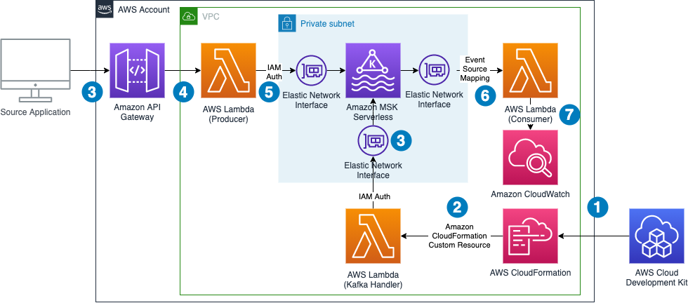
The data flow contains the following steps:
- The infrastructure is defined in an AWS CDK application. By running this application, a set of AWS CloudFormation templates is created.
- AWS CloudFormation creates all infrastructure components, including a Lambda function that runs during the deployment process to create a topic in the MSK Serverless cluster and to retrieve the authentication endpoint needed for the producer Lambda function. On destruction of the CloudFormation stack, the same Lambda function gets triggered again to delete the topic from the cluster.
- An external application calls an API Gateway endpoint.
- API Gateway forwards the request to a Lambda function.
- The Lambda function acts as a Kafka producer and pushes the message to a Kafka topic using IAM authentication.
- The Lambda event source mapping mechanism triggers the Lambda consumer function and forwards the message to it.
- The Lambda consumer function logs the data to Amazon CloudWatch.
Note that we don’t need to worry about Availability Zones. MSK Serverless automatically replicates the data across multiple Availability Zones to ensure high availability of the data.
The demo additionally shows how to use Lambda Powertools for Java to streamline logging and tracing and the IAM authenticator for the simple authentication process outlined in the introduction.
The following sections take you through the steps to deploy, test, and observe the example application.
Prerequisites
The example has the following prerequisites:
- An AWS account. If you haven’t signed up, complete the following steps:
- Create an account. For instructions, see Sign Up For AWS.
- Create an IAM user. For instructions, see Create IAM User.
- The following software installed on your development machine, or use an AWS Cloud9 environment, which comes with all requirements preinstalled:
- Java Development Kit 17 or higher (for example, Amazon Corretto 17, OpenJDK 17)
- Python version 3.11 or higher
- Apache Maven version 3.8.4 or higher
- Docker version 24.0.2 or higher
- Node.js v18.0.0
- AWS CLI 2.12.1 or higher
- AWS CDK 2.89.0 or higher
- Appropriate AWS credentials for interacting with resources in your AWS account.
Deploy the solution
Complete the following steps to deploy the solution:
- Clone the project GitHub repository and change the directory to subfolder
serverless-kafka-iac:
- Configure environment variables:
- Prepare the virtual Python environment:
- Bootstrap your account for AWS CDK usage:
- Run cdk synth to build the code and test the requirements (ensure docker daemon is running on your machine):
- Run cdk deploy to deploy the code to your AWS account:
Test the solution
To test the solution, we generate messages for the Kafka topics by sending calls through the API Gateway from our development machine or AWS Cloud9 environment. We then go to the CloudWatch console to observe incoming messages in the log files of the Lambda consumer function.
- Open a terminal on your development machine to test the API with the Python script provided under
/serverless\_kafka\_iac/test\_api.py:
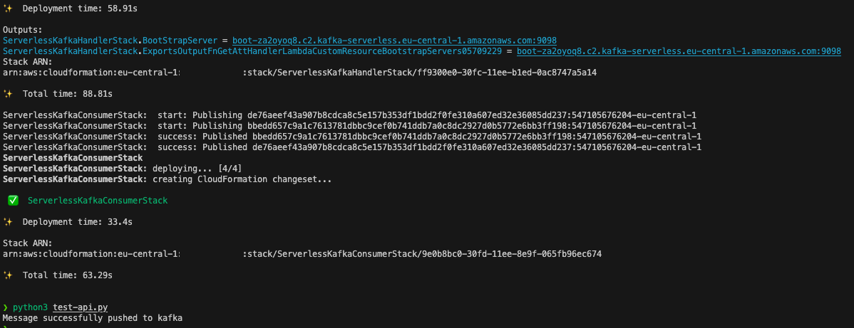
- On the Lambda console, open the Lambda function named
ServerlessKafkaConsumer.
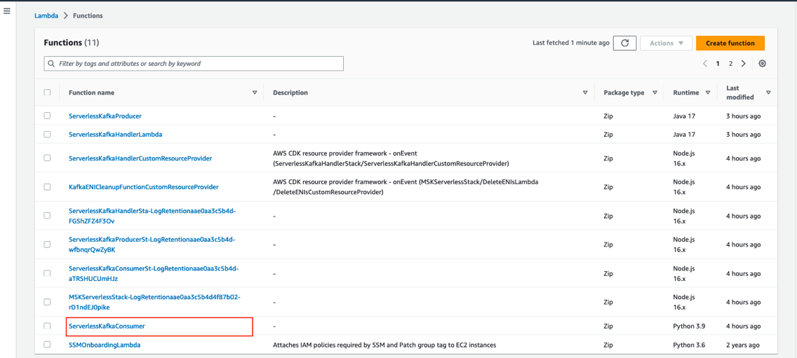
- On the Monitor tab, choose View CloudWatch logs to access the logs of the Lambda function.
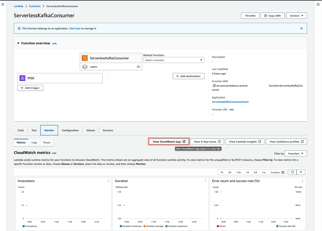
- Choose the latest log stream to access the log files of the last run.
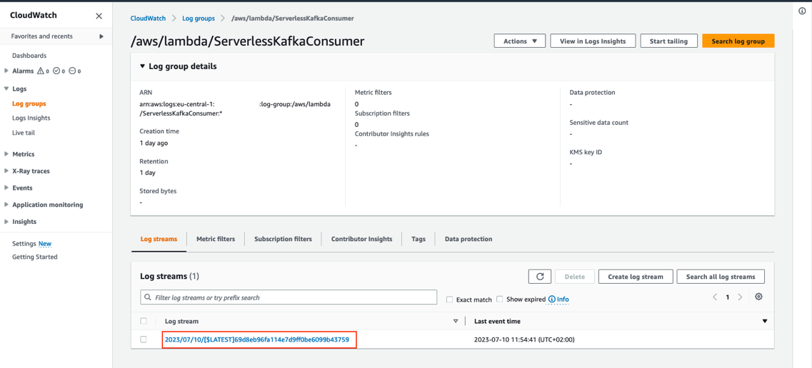
You can review the log entry of the received Kafka messages in the log of the Lambda function.
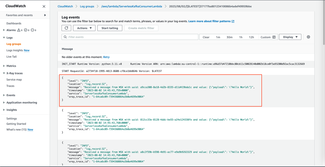
Trace a request
All components integrate with AWS X-Ray. With AWS X-Ray, you can trace the entire application, which is useful to identify bottlenecks when load testing. You can also trace method runs at the Java method level.
Lambda Powertools for Java allows you to shortcut this process by adding the @Trace annotation to a method to see traces on the method level in X-Ray.
To trace a request end to end, complete the following steps:
- On the CloudWatch console, choose Service map in the navigation pane.
- Select a component to investigate (for example, the Lambda function where you deployed the Kafka producer).
- Choose View traces.
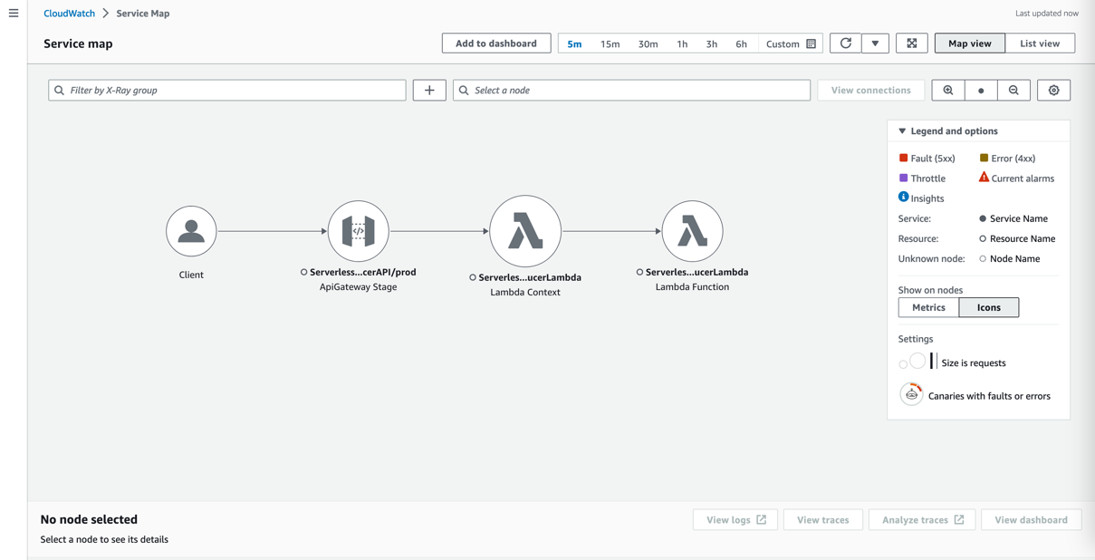
- Choose a single Lambda method invocation and investigate further at the Java method level.
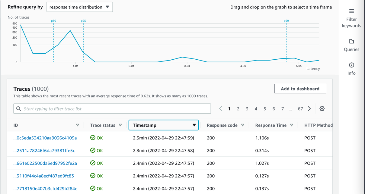
Implement a Kafka producer in Lambda
Kafka natively supports Java. To stay open, cloud native, and without third-party dependencies, the producer is written in that language. Currently, the IAM authenticator is only available to Java. In this example, the Lambda handler receives a message from an API Gateway source and pushes this message to an MSK topic called messages.
Typically, Kafka producers are long-living and pushing a message to a Kafka topic is an asynchronous process. Because Lambda is ephemeral, you must enforce a full flush of a submitted message until the Lambda function ends by calling producer.flush():
Connect to Amazon MSK using IAM authentication
This post uses IAM authentication to connect to the respective Kafka cluster. For information about how to configure the producer for connectivity, refer to IAM access control.
Because you configure the cluster via IAM, grant Connect and WriteData permissions to the producer so that it can push messages to Kafka:
This shows the Kafka excerpt of the IAM policy, which must be applied to the Kafka producer. When using IAM authentication, be aware of the current limits of IAM Kafka authentication, which affect the number of concurrent connections and IAM requests for a producer. Refer to Amazon MSK quota and follow the recommendation for authentication backoff in the producer client:
Additional considerations
Each MSK Serverless cluster can handle 100 requests per second. To reduce IAM authentication requests from the Kafka producer, place it outside of the handler. For frequent calls, there is a chance that Lambda reuses the previously created class instance and only reruns the handler.
For bursting workloads with a high number of concurrent API Gateway requests, this can lead to dropped messages. Although this might be tolerable for some workloads, for others this might not be the case.
In these cases, you can extend the architecture with a buffering technology like Amazon Simple Queue Service (Amazon SQS) or Amazon Kinesis Data Streams between API Gateway and Lambda.
To reduce latency, reduce cold start times for Java by changing the tiered compilation level to 1, as described in Optimizing AWS Lambda function performance for Java. Provisioned concurrency ensures that polling Lambda functions don’t need to warm up before requests arrive.
Conclusion
In this post, we showed how to create a serverless integration Lambda function between API Gateway and MSK Serverless as a way to do IAM authentication when your producer is not written in Java. You also learned about the native integration of Lambda and Amazon MSK on the consumer side. Additionally, we showed how to deploy such an integration with the AWS CDK.
The general pattern is suitable for many use cases where you want to use IAM authentication but your producers or consumers are not written in Java, but you still want to take advantage of the benefits of MSK Serverless, like its ability to scale up and down with unpredictable or spikey workloads or its little to no operational overhead of running Apache Kafka.
You can also use MSK Serverless to reduce operational complexity by automating provisioning and the management of capacity needs, including the need to constantly monitor brokers and storage.
For more serverless learning resources, visit Serverless Land.
For more information on MSK Serverless, check out the following:
- MSK Serverless Developer Guide
- Building a Serverless Apache Kafka Data Pipeline workshop
- Split your monolith Apache clusters using Amazon MSK Serverless
- Connect to Amazon MSK Serverless from your on-premises network
About the Authors
 Philipp Klose is a Global Solutions Architect at AWS based in Munich. He works with enterprise FSI customers and helps them solve business problems by architecting serverless platforms. In this free time, Philipp spends time with his family and enjoys every geek hobby possible.
 Daniel Wessendorf is a Global Solutions Architect at AWS based in Munich. He works with enterprise FSI customers and is primarily specialized in machine learning and data architectures. In his free time, he enjoys swimming, hiking, skiing, and spending quality time with his family.
 Marvin Gersho is a Senior Solutions Architect at AWS based in New York City. He works with a wide range of startup customers. He previously worked for many years in engineering leadership and hands-on application development, and now focuses on helping customers architect secure and scalable workloads on AWS with a minimum of operational overhead. In his free time, Marvin enjoys cycling and strategy board games.
 Nathan Lichtenstein is a Senior Solutions Architect at AWS based in New York City. Primarily working with startups, he ensures his customers build smart on AWS, delivering creative solutions to their complex technical challenges. Nathan has worked in cloud and network architecture in the media, financial services, and retail spaces. Outside of work, he can often be found at a Broadway theater.
OpenSearch is an open-source RESTful search engine built on top of the Apache Lucene library. OpenSearch full-text search is fast, can give the result of complex queries within a fraction of a second. With OpenSearch, you can convert unstructured text into structured text using different text analyzers, tokenizers, and filters to improve search. OpenSearch uses a default analyzer, called the standard analyzer, which works well for most use cases out of the box. But for some use cases, it may not work best, and you need to use a specific analyzer.
In this post, we show how you can implement a suffix-based search. To find a document with the movie name “saving private ryan” for example, you can use the prefix “saving” with a prefix-based query. Occasionally, you also want to match suffixes as well, such as matching “Harry Potter Goblet of Fire” with the suffix “Fire” To do that, first reverse the string “eriF telboG rettoP yrraH” with the reverse token filter, then query for the prefix “eriF”.
Solution overview
Text analysis involves transforming unstructured text, such as the content of an email or a product description, into a structured format that is finely tuned for effective searching. An analyzer enables the implementation of full-text search using tokenization, which entails breaking down a text into smaller fragments known as tokens, with these tokens commonly representing individual words. To implement a reversed field search, the analyzer does the following.

The analyzer processes text in the following order:
- Use a character filter to replace
-with\_. For example, from “My Driving License Number Is 123-456-789” to “My Driving License Number Is 123\_456\_789.” - The standard tokenizer splits texts into tokens. For example, from “My Driving License Number Is 123\_456\_789” to “[ my, driving, license, number, is, 123, 456, 789 ].”
- The reverse token filter reverses each token in a stream. For example, from [ my, driving, license, number, is, 123, 456, 789 ] to [ ym, gnivird, esnecil, rebmun, si, 321, 654, 987 ].
The standard analyzer (default analyzer) breaks down input strings into tokens based on word boundaries and removes most punctuation marks. For additional information about analyzers, refer Build-in analyzers.
Indexing and searching
Every document is a collection of fields, each having its own specific data type. When you create a mapping for your data, you create a mapping definition, which contains a list of fields that are pertinent to the document. To know more about index mappings refer to index mapping.
Let’s take the example of an analyzer with the reverse token filter applied on the text field.
- First, create an index with mappings as shown in the following code. The new field ‘
reverse\_title’ is derived from ‘title’ field for suffix search and original field ‘title’ will be used for normal search.
- Insert some documents into the index:
- Run the following query to perform a suffix/reverse search on derived field ‘
reverse\_title’ for “Fire”:
The following code shows our results:
- For non-reverse search you can use original field ‘
title’.
The following code shows our result.
The query returns a document with the movie name “Harry Potter Goblet of Fire”.
If you’re curious to know how search works at high level, refer to A query, or There and Back Again.
Conclusion
In this post, you walked through how text analysis works in OpenSearch and how to implement suffix-based search using a reverse token filter effectively.
If you have feedback about this post, submit your comments in the comments section.
About the Authors
 Bharav Patel is a Specialist Solution Architect, Analytics at Amazon Web Services. He primarily works on Amazon OpenSearch Service and helps customers with key concepts and design principles of running OpenSearch workloads on the cloud. Bharav likes to explore new places and try out different cuisines.
Amazon Redshift is a fully managed, petabyte-scale data warehouse service in the cloud. With Amazon Redshift, you can analyze all your data to derive holistic insights about your business and your customers. It supports stored procedures where prepared SQL code is saved and the code can be reused over and over again.
Stored procedures are commonly used to encapsulate logic for data transformation, data validation, and business-specific logic. By combining multiple SQL steps into a stored procedure, you can create reusable code blocks that can run together as a single transaction or multiple individual transactions. You can also schedule stored procedures to automate data processing on Amazon Redshift. For more information, refer to Bringing your stored procedures to Amazon Redshift.
In the Redshift stored procedure default atomic transaction mode, a call to a Redshift stored procedure will create its own transaction when the call starts or is part of the existing transaction if an explicit transaction is opened before the stored procedure is called. All the statements inside a procedure behave as if they are in a single transaction block that ends when the stored procedure call finishes. A nested call to another procedure is treated like any other SQL statement and operates within the context of the same transaction as the caller. Statements for TRUNCATE, COMMIT, and ROLLBACK and the exception handling block with arbitrary SQL statements close the current transaction and start a new transaction implicitly. This behavior can cause challenges in migration to Amazon Redshift from other systems like Teradata.
In this post, we discuss the enhancements to Amazon Redshift stored procedures for non-atomic transaction mode. This mode provides enhanced transaction controls that enable you to automatically commit the statements inside the stored procedure.
Non-atomic transaction mode
The new non-atomic transaction mode feature provides three enhancements on stored procedures in Amazon Redshift:
- Unless the DML or DDL statements are part of an explicit open transaction, each statement in the stored procedure will run in its own implicit transaction and a new transaction will be opened to handle following statements. If an explicit transaction is opened, then all subsequent statements are run and remain un-committed until an explicit transaction control command (COMMIT or ROLLBACK) is run to end the transaction.
- Amazon Redshift will not re-raise the exception after the exception handler statements are complete. Therefore, a new RAISE statement without any INFO or EXCEPTION has been provided to re-throw the exception caught by the exception handling block. This RAISE statement without any INFO or EXCEPTION will only be allowed in the exception handling block.
- Also, the new START TRANSACTION statement begins an explicit transaction inside the non-atomic transaction mode stored procedure. Use the existing transaction control command (COMMIT or ROLLBACK) to end the explicitly started transaction.
- Amazon Redshift does not support sub-transactions so if there is already an open transaction, then calling this statement again will do nothing, and no error is raised.
- If an explicit transaction is still open when the nonatomic transaction mode stored procedure call ends, then the explicit transaction remains open until a transaction control command is run in the session.
- If the session disconnects before running a transaction control command, the whole transaction is automatically rolled back.
Additional restrictions
Some restrictions have also been introduced for Redshift stored procedures:
- For nesting stored procedure calls, all the procedures must be created in the same transaction mode, no matter if it’s in atomic (default) transaction mode or the new non-atomic transaction mode
- You can’t nest stored procedures across the two transaction modes (atomic and non-atomic)
- You can’t set the SECURITY DEFINER option or SET
configuration\_parameteroption for non-atomic transaction mode stored procedures
Impact to cursors
Cursors in non-atomic transaction mode stored procedures will behave differently compared to the default atomic transaction mode:
- Cursor statements will need an explicit transaction block before beginning the cursor to ensure that each iteration of the cursor loop is not auto-committed.
- To return a cursor from non-atomic transaction mode stored procedure, you will need an explicit transaction block before beginning the cursor. Otherwise, the cursor will be closed when the SQL statement inside the loop is automatically committed.
Advantages
The following are key advantages of this feature from a user perspective:
- It provides the capability to lift and shift Teradata stored procedures to run in Teradata session mode. This helps in seamless migrations from traditional data warehouses like Teradata and SQL Server.
- It enables Amazon Redshift to provide more flexible operations inside of stored procedures when encountering errors and exceptions. Amazon Redshift can now preserve previous action’s state before reaching an exception.
Syntax
The new optional keyword NONATOMIC has been added to the stored procedure definition syntax, as shown in the following code:
This optional keyword creates the stored procedure under the non-atomic transaction mode. If you don’t specify the keyword, then the default atomic mode will be the transaction mode when creating the stored procedure.
NONATOMIC means each DML and DDL statement in the procedure will be implicitly committed.
Without non-atomic mode, the procedure will create its own transaction when the call starts or be part of the existing transaction if an explicit transaction is opened before it is called. Every statement within the stored procedure will belong to this one transaction.
Example of NONATOMIC mode
Let’s consider the customer contact table custcontacts, which stores customer primary and secondary contact phone numbers:
We insert three sample customer records with no contact values:
You need to create a stored procedure to update the primary and secondary phone numbers. The requirement is not to roll back updates to the primary contact number if updates to the secondary contact number fail for some reason.
You can achieve this by creating the stored procedure with the NONATOMIC keyword. The NONATOMIC keyword ensures that each statement in the stored procedure runs in its own implicit transaction block. Therefore, if the UPDATE statement for the secondary phone fails, then it won’t roll back the data update made to the primary phone. See the following code:
Now let’s call the stored procedure passing the secondary phone number with more than 10 digits, which will fail in the secondaryphone UPDATE statement due to incorrect length:
The preceding procedure call will update the primary phone number successfully. The secondary phone number update fails. However, the primaryphone update will not roll back because it ran in its own implicit transaction block due to the NONATOMIC clause in the stored procedure definition.
Exception handling in NONATOMIC mode
Exceptions are handled in stored procedures differently based on the atomic or non-atomic mode:
- Atomic (default) – Exceptions are always re-raised
- Non-atomic – Exceptions are handled and you can choose to re-raise or not
Let’s continue with the previous example to illustrate exception handling in non-atomic mode.
Create the following table to log exceptions raised by stored procedures:
Now update the sp\_update\_custcontacts() procedure to handle exceptions. Note that we’re adding an EXCEPTION block in the procedure definition. It inserts a record in the procedure\_log table in the event of an exception.
Now create one more stored procedure, which will call the preceding procedure. It also has an EXCEPTION block and inserts a record in the procedure\_log table in the event of an exception.
Let’s call the parent procedure we created:
This in turn will call the sp\_update\_custcontacts() procedure. The inner procedure sp\_update\_custcontacts() will fail because we’re updating the secondary phone with an invalid value. The control will enter the EXCEPTION block of the sp\_update\_custcontacts() procedure and make an insert into the procedure\_log table.
However, it will not re-raise the exception in non-atomic mode. Therefore, the parent procedure sp\_update\_customer() will not get the exception passed from the sp\_update\_custcontacts() procedure. The control will not enter the EXCEPTION block of the sp\_update\_customer() procedure.
If you query the procedure\_log table, you will see an entry only for the error handled by the sp\_update\_custcontacts() procedure:

Now redefine the sp\_update\_custcontacts() procedure with the RAISE statement:
Let’s call the parent stored procedure sp\_update\_customer() again:
Now the inner procedure sp\_update\_custcontacts() will re-raise the exception to the parent procedure sp\_update\_customer() after handling the exception in its own EXCEPTION block. Then the control will reach the EXCEPTION block in the parent procedure and insert another record into the procedure\_log table.
If you query the procedure\_log table now, you will see two entries: one by the inner procedure sp\_update\_custcontacts() and another by the parent procedure sp\_update\_customer(). This demonstrates that the RAISE statement in the inner procedure re-raised the exception.

Explicit START TRANSACTION statement in non-atomic mode
You can issue a START TRANSACTION statement to begin a transaction block inside the stored procedure. It will open a new transaction inside the stored procedure. For examples, refer to Nonatomic mode stored procedure transaction management.
Conclusion
In this post, we discussed the enhancements to Redshift stored procedures for non-atomic transaction mode, which provides enhanced transaction controls to enable you to automatically commit the statements inside the stored procedure. This mode also enables easier migration to Amazon Redshift from other systems like Teradata. Try out these enhancements and let us know your experience in comments.
About the Authors
 Milind Oke is a Data Warehouse Specialist Solutions Architect based out of New York. He has been building data warehouse solutions for over 15 years and specializes in Amazon Redshift.
 Satesh Sonti is a Sr. Analytics Specialist Solutions Architect based out of Atlanta, specialized in building enterprise data platforms, data warehousing, and analytics solutions. He has over 17 years of experience in building data assets and leading complex data platform programs for banking and insurance clients across the globe.
 Kiran Chinta is a Software Development Manager at Amazon Redshift. He leads a strong team in query processing, SQL language, data security, and performance. Kiran is passionate about delivering products that seamlessly integrate with customers’ business applications with the right ease of use and performance. In his spare time, he enjoys reading and playing tennis.
 Huichen Liu is a software development engineer on the Amazon Redshift query processing team. She focuses on query optimization, statistics and SQL language features. In her spare time, she enjoys hiking and photography.
Ingesting a high volume of streaming data has been a defining characteristic of operational analytics workloads with Amazon OpenSearch Service. Many of these workloads involve either self-managed Apache Kafka or Amazon Managed Streaming for Apache Kafka (Amazon MSK) to satisfy their data streaming needs. Consuming data from Amazon MSK and writing to OpenSearch Service has been a challenge for customers. AWS Lambda, custom code, Kafka Connect, and Logstash have been used for ingesting this data. These methods involve tools that must be built and maintained. In this post, we introduce Amazon MSK as a source to Amazon OpenSearch Ingestion, a serverless, fully managed, real-time data collector for OpenSearch Service that makes this ingestion even easier.
Solution overview
The following diagram shows the flow from data sources to Amazon OpenSearch Service.
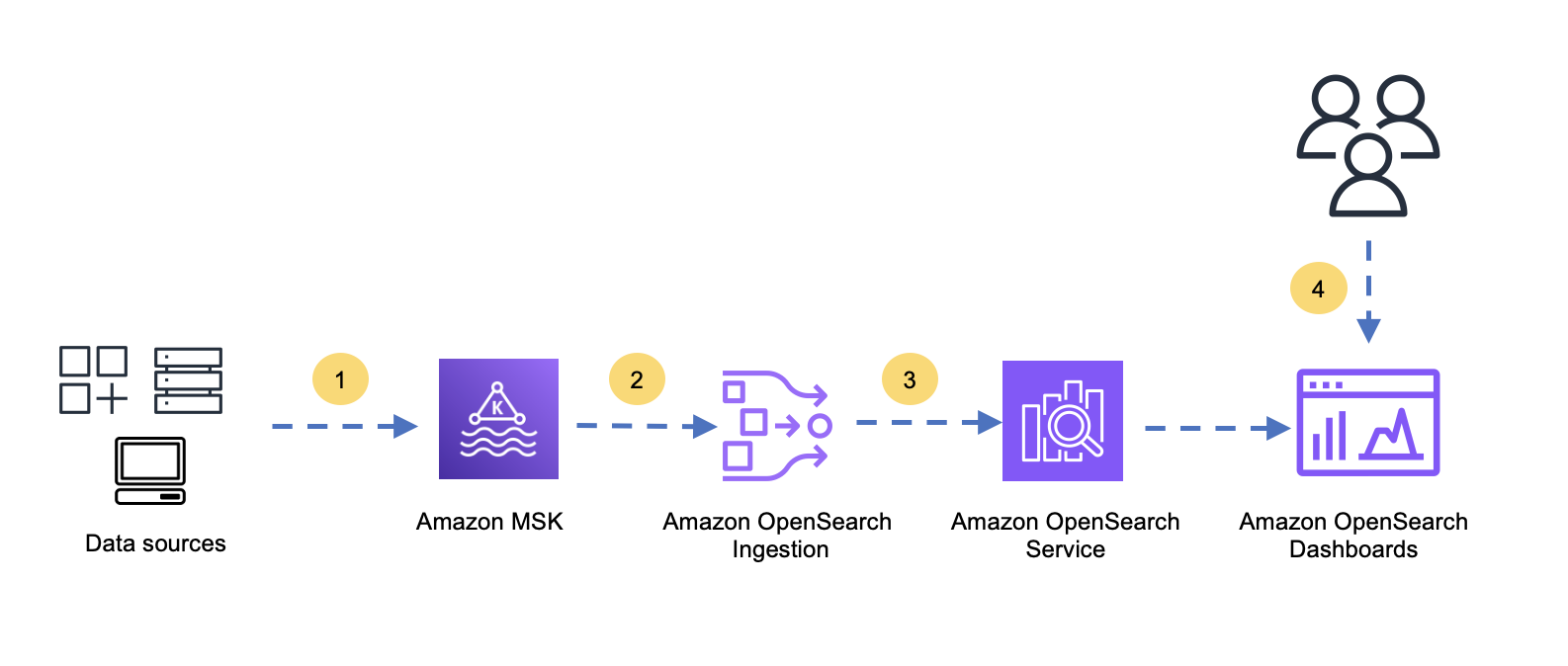
The flow contains the following steps:
- Data sources produce data and send that data to Amazon MSK
- OpenSearch Ingestion consumes the data from Amazon MSK.
- OpenSearch Ingestion transforms, enriches, and writes the data into OpenSearch Service.
- Users search, explore, and analyze the data with OpenSearch Dashboards.
Prerequisites
You will need a provisioned MSK cluster created with appropriate data sources. The sources, as producers, write data into Amazon MSK. The cluster should be created with the appropriate Availability Zone, storage, compute, security and other configurations to suit your workload needs. To provision your MSK cluster and have your sources producing data, see Getting started using Amazon MSK.
As of this writing, OpenSearch Ingestion supports Amazon MSK provisioned, but not Amazon MSK Serverless. However, OpenSearch Ingestion can reside in the same or different account where Amazon MSK is present. OpenSearch Ingestion uses AWS PrivateLink to read data, so you must turn on multi-VPC connectivity on your MSK cluster. For more information, see Amazon MSK multi-VPC private connectivity in a single Region. OpenSearch Ingestion can write data to Amazon Simple Storage Service (Amazon S3), provisioned OpenSearch Service, and Amazon OpenSearch Service. In this solution, we use a provisioned OpenSearch Service domain as a sink for OSI. Refer to Getting started with Amazon OpenSearch Service to create a provisioned OpenSearch Service domain. You will need appropriate permission to read data from Amazon MSK and write data to OpenSearch Service. The following sections outline the required permissions.
Permissions required
To read from Amazon MSK and write to Amazon OpenSearch Service, you need to create a an AWS Identity and Access Management (IAM) role used by Amazon OpenSearch Ingestion. In this post we use a role called pipeline-Role for this purpose. To create this role please see Creating IAM roles.
Reading from Amazon MSK
OpenSearch Ingestion will need permission to create a PrivateLink connection and other actions that can be performed on your MSK cluster. Edit your MSK cluster policy to include the following snippet with appropriate permissions. If your OpenSearch Ingestion pipeline resides in an account different from your MSK cluster, you will need a second section to allow this pipeline. Use proper semantic conventions when providing the cluster, topic, and group permissions and remove the comments from the policy before using.
Edit the pipeline role’s inline policy to include the following permissions. Ensure that you have removed the comments before using the policy.
Writing to OpenSearch Service
In this section, you provide the pipeline role with necessary permissions to write to OpenSearch Service. As a best practice, we recommend using fine-grained access control in OpenSearch Service. Use OpenSearch dashboards to map a pipeline role to an appropriate backend role. For more information on mapping roles to users, see Managing permissions. For example, all\_access is a built-in role that grants administrative permission to all OpenSearch functions. When deploying to a production environment, ensure that you use a role with enough permissions to write to your OpenSearch domain.

Creating OpenSearch Ingestion pipelines
The pipeline role now has the correct set of permissions to read from Amazon MSK and write to OpenSearch Service. Navigate to the OpenSearch Service console, choose Pipelines, then choose Create pipeline.
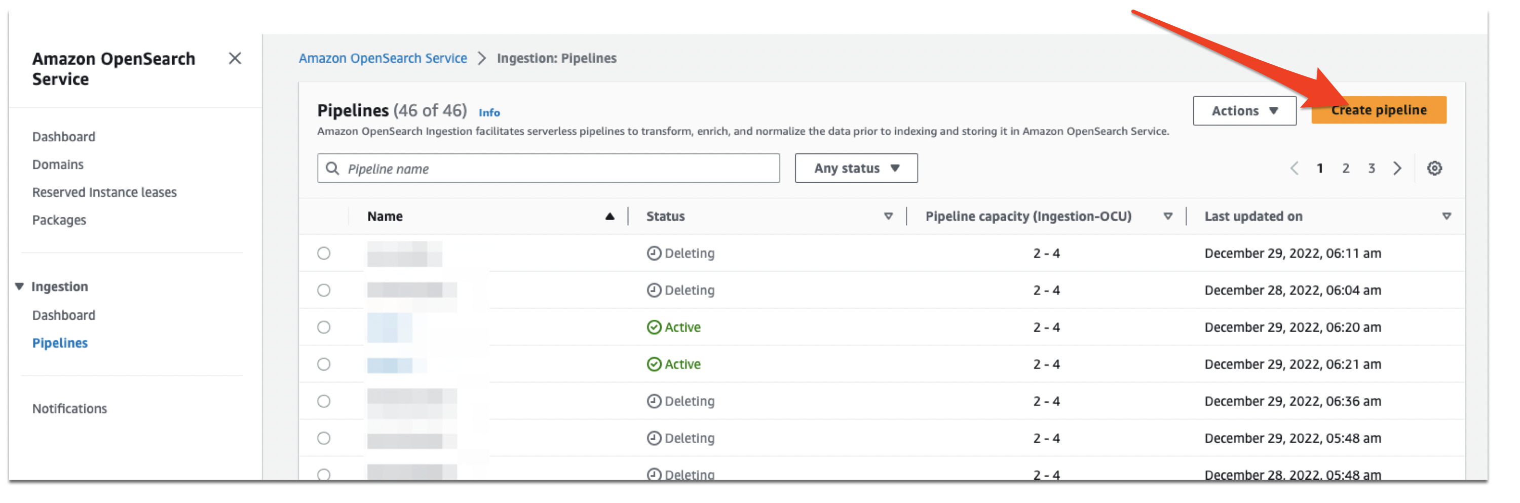
Choose a suitable name for the pipeline. and se the pipeline capacity with appropriate minimum and maximum OpenSearch Compute Unit (OCU). Then choose ‘AWS-MSKPipeline’ from the dropdown menu as shown below.
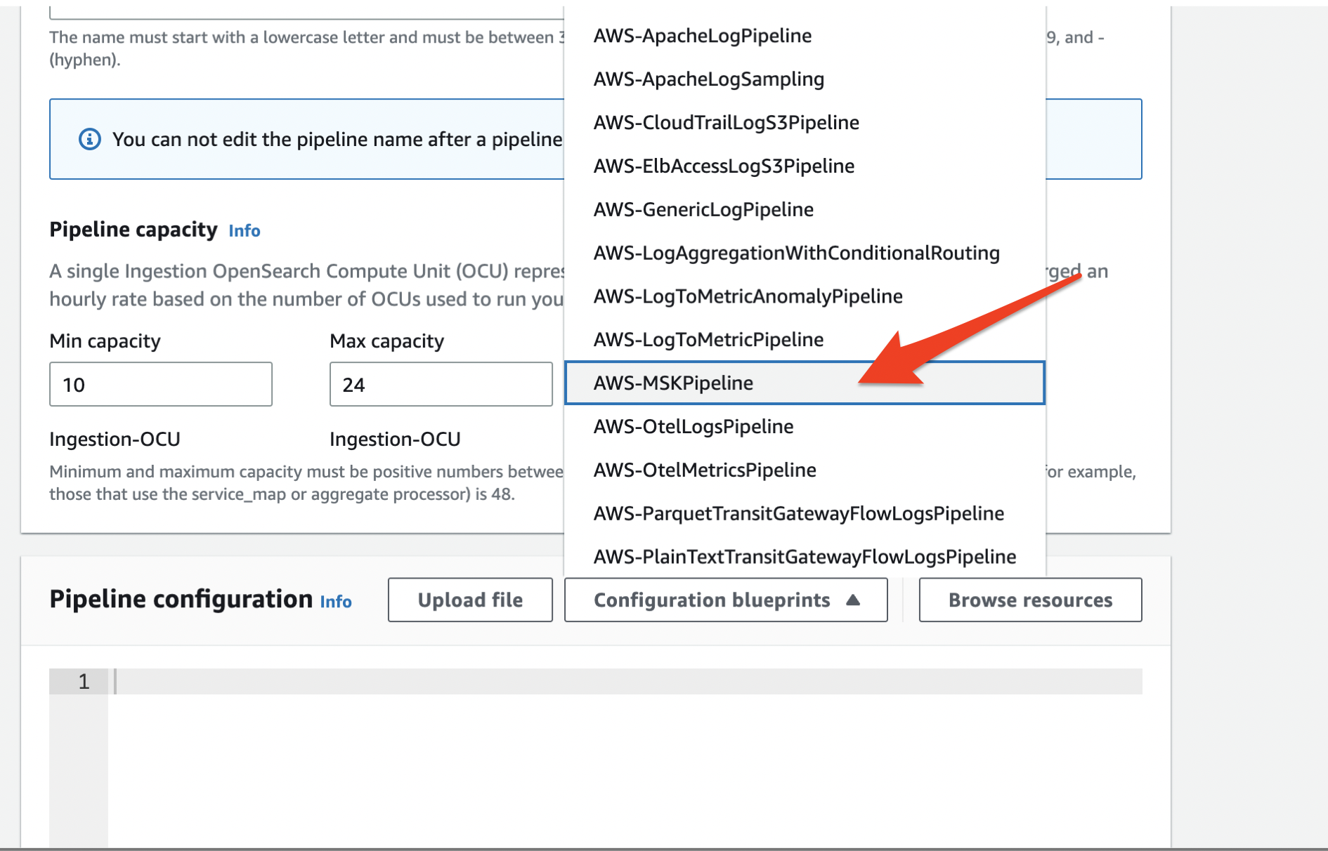
Use the provided template to fill in all the required fields. The snippet in the following section shows the fields that needs to be filled in red.
Configuring Amazon MSK source
The following sample configuration snippet shows every setting you need to get the pipeline running:
We use the following parameters:
- acknowledgements – Set to
truefor OpenSearch Ingestion to ensure that the data is delivered to the sinks before committing the offsets in Amazon MSK. The default value is set to false. - name – This specifies topic OpenSearch Ingestion can read from. You can read a maximum of four topics per pipeline.
- group\_id – This parameter specifies that the pipeline is part of the consumer group. With this setting, a single consumer group can be scaled to as many pipelines as needed for very high throughput.
- serde\_format – Specifies a deserialization method to be used for the data read from Amazon MSK. The options are JSON and plaintext.
- AWS sts\_role\_arn and OpenSearch sts\_role\_arn – Specifies the role OpenSearch Ingestion uses for reading and writing. Specify the ARN of the role you created from the last section. OpenSearch Ingestion currently uses the same role for reading and writing.
- MSK arn – Specifies the MSK cluster to consume data from.
- OpenSearch host and index – Specifies the OpenSearch domain URL and where the index should write.
When you have configured the Kafka source, choose the network access type and log publishing options. Public pipelines do not involve PrivateLink and they will not incur a cost associated with PrivateLink. Choose Next and review all configurations. When you are satisfied, choose Create pipeline.
Log in to OpenSearch Dashboards to see your indexes and search the data.
Recommended compute units (OCUs) for the MSK pipeline
Each compute unit has one consumer per topic. Brokers will balance partitions among these consumers for a given topic. However, when the number of partitions is greater than the number of consumers, Amazon MSK will host multiple partitions on every consumer. OpenSearch Ingestion has built-in auto scaling to scale up or down based on CPU usage or number of pending records in the pipeline. For optimal performance, partitions should be distributed across many compute units for parallel processing. If topics have a large number of partitions, for example, more than 96 (maximum OCUs per pipeline), we recommend configuring a pipeline with 1–96 OCUs because it will auto scale as needed. If a topic has a low number of partitions, for example, less than 96, then keep the maximum compute unit to same as the number of partitions. When pipeline has more than one topic, user can pick a topic with highest number of partitions as a reference to configure maximum computes units. By adding another pipeline with a new set of OCUs to the same topic and consumer group, you can scale the throughput almost linearly.
Clean up
To avoid future charges, clean up any unused resources from your AWS account.
Conclusion
In this post, you saw how to use Amazon MSK as a source for OpenSearch Ingestion. This not only addresses the ease of data consumption from Amazon MSK, but it also relieves you of the burden of self-managing and manually scaling consumers for varying and unpredictable high-speed, streaming operational analytics data. Please refer to the ‘sources’ list under ‘supported plugins’ section for exhaustive list of sources from which you can ingest data.
About the authors
 Muthu Pitchaimani is a Search Specialist with Amazon OpenSearch Service. He builds large-scale search applications and solutions. Muthu is interested in the topics of networking and security, and is based out of Austin, Texas.
 Arjun Nambiar is a Product Manager with Amazon OpenSearch Service. He focusses on ingestion technologies that enable ingesting data from a wide variety of sources into Amazon OpenSearch Service at scale. Arjun is interested in large scale distributed systems and cloud-native technologies and is based out of Seattle, Washington.
 Raj Sharma is a Sr. SDM with Amazon OpenSearch Service. He builds large-scale distributed applications and solutions. Raj is interested in the topics of Analytics, databases, networking and security, and is based out of Palo Alto, California.
Amazon Redshift is a fast, fully managed petabyte-scale cloud data warehouse that makes it simple and cost-effective to analyze all your data using standard SQL and your existing business intelligence (BI) tools. Tens of thousands of customers today use Amazon Redshift to analyze exabytes of data and run analytical queries, making it the most widely used cloud data warehouse. Amazon Redshift is available in both serverless and provisioned configurations.
Amazon Redshift enables you to directly access data stored in Amazon Simple Storage Service (Amazon S3) using SQL queries and join data across your data warehouse and data lake. With Amazon Redshift, you can query the data in your S3 data lake using a central AWS Glue metastore from your Redshift data warehouse.
Amazon Redshift supports querying a wide variety of data formats, such as CSV, JSON, Parquet, and ORC, and table formats like Apache Hudi and Delta. Amazon Redshift also supports querying nested data with complex data types such as struct, array, and map.
With this capability, Amazon Redshift extends your petabyte-scale data warehouse to an exabyte-scale data lake on Amazon S3 in a cost-effective manner.
Apache Iceberg is the latest table format that is supported now in preview by Amazon Redshift. In this post, we show you how to query Iceberg tables using Amazon Redshift, and explore Iceberg support and options.
Solution overview
Apache Iceberg is an open table format for very large petabyte-scale analytic datasets. Iceberg manages large collections of files as tables, and it supports modern analytical data lake operations such as record-level insert, update, delete, and time travel queries. The Iceberg specification allows seamless table evolution such as schema and partition evolution, and its design is optimized for usage on Amazon S3.
Iceberg stores the metadata pointer for all the metadata files. When a SELECT query is reading an Iceberg table, the query engine first goes to the Iceberg catalog, then retrieves the entry of the location of the latest metadata file, as shown in the following diagram.
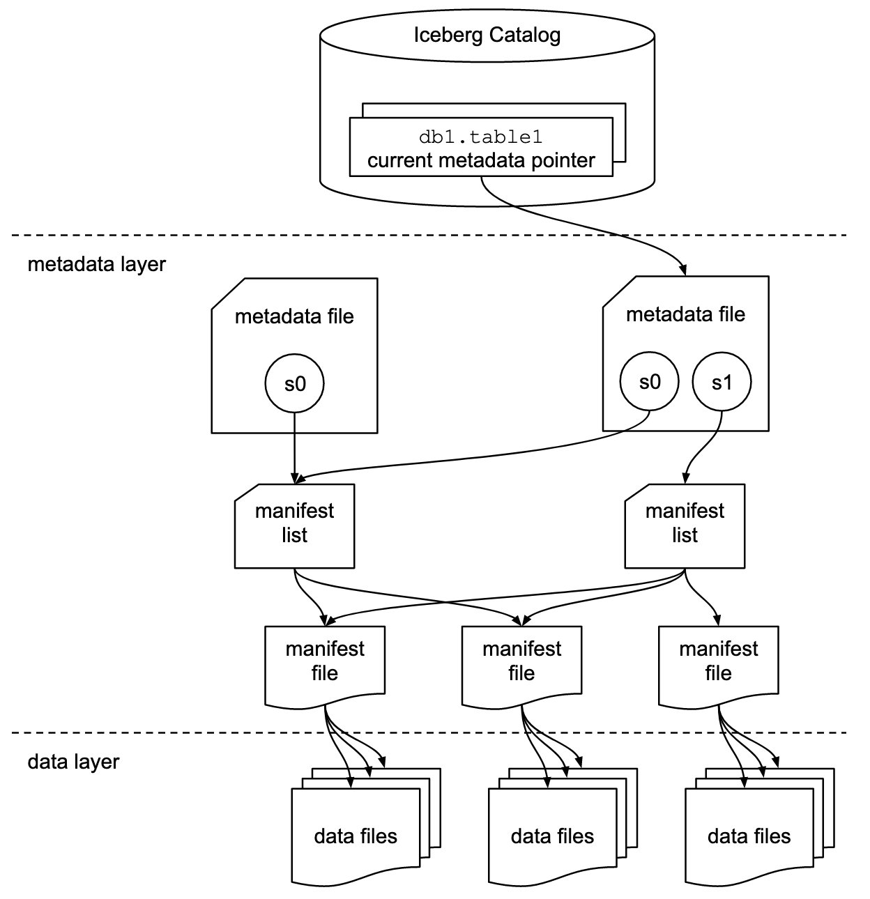
Amazon Redshift now provides support for Apache Iceberg tables, which allows data lake customers to run read-only analytics queries in a transactionally consistent way. This enables you to easily manage and maintain your tables on transactional data lakes.
Amazon Redshift supports Apache Iceberg’s native schema and partition evolution capabilities using the AWS Glue Data Catalog, eliminating the need to alter table definitions to add new partitions or to move and process large amounts of data to change the schema of an existing data lake table. Amazon Redshift uses the column statistics stored in the Apache Iceberg table metadata to optimize its query plans and reduce the file scans required to run queries.
In this post, we use the Yellow taxi public dataset from NYC Taxi & Limousine Commission as our source data. The dataset contains data files in Apache Parquet format on Amazon S3. We use Amazon Athena to convert this Parquet dataset and then use Amazon Redshift Spectrum to query and join with a Redshift local table, perform row-level deletes and updates and partition evolution, all coordinated through the AWS Glue Data Catalog in an S3 data lake.
Prerequisites
You should have the following prerequisites:
- An AWS account. If you don’t have one, you can sign up for one.
- A Redshift cluster with the current track version. For setup instructions, see Create a sample Amazon Redshift cluster.
- Alternatively, you could use an Amazon Redshift Serverless endpoint. For setup instructions, see Getting started with Amazon Redshift Serverless.
- An AWS Identity and Access Management (IAM) role set up for Redshift data lake access.
- An S3 bucket to store Parquet and Iceberg files.
- An Athena workgroup with Athena engine version 3 to use CTAS and MERGE commands with an Apache Iceberg table. To upgrade your existing Athena engine to version 3 in your Athena workgroup, follow the instructions in Upgrade to Athena engine version 3 to increase query performance and access more analytics features or refer to Changing the engine version in the Athena console.
Convert Parquet data to an Iceberg table
For this post, you need the Yellow taxi public dataset from the NYC Taxi & Limousine Commission available in Iceberg format. You can download the files and then use Athena to convert the Parquet dataset into an Iceberg table, or refer to Build an Apache Iceberg data lake using Amazon Athena, Amazon EMR, and AWS Glue blog post to create the Iceberg table.
In this post, we use Athena to convert the data. Complete the following steps:
- Download the files using the previous link or use the AWS Command Line Interface (AWS CLI) to copy the files from the public S3 bucket for year 2020 and 2021 to your S3 bucket using the following command:
For more information, refer to Setting up the Amazon Redshift CLI.
- Create a database
Icebergdband create a table using Athena pointing to the Parquet format files using the following statement: - Validate the data in the Parquet table using the following SQL:

- Create an Iceberg table in Athena with the following code. You can see the table type properties as an Iceberg table with Parquet format and snappy compression in the following
create tablestatement. You need to update the S3 location before running the SQL. Also note that the Iceberg table is partitioned with theYearkey. - After you create the table, load the data into the Iceberg table using the previously loaded Parquet table
nyc\_taxi\_yellow\_parquetwith the following SQL: - When the SQL statement is complete, validate the data in the Iceberg table
nyc\_taxi\_yellow\_iceberg. This step is required before moving to the next step. - You can validate that the nyc\_taxi\_yellow\_iceberg table is in Iceberg format table and partitioned on the Year column using the following command:


Create an external schema in Amazon Redshift
In this section, we demonstrate how to create an external schema in Amazon Redshift pointing to the AWS Glue database icebergdb to query the Iceberg table nyc\_taxi\_yellow\_iceberg that we saw in the previous section using Athena.
Log in to the Redshift via Query Editor v2 or a SQL client and run the following command (note that the AWS Glue database icebergdb and Region information is being used):
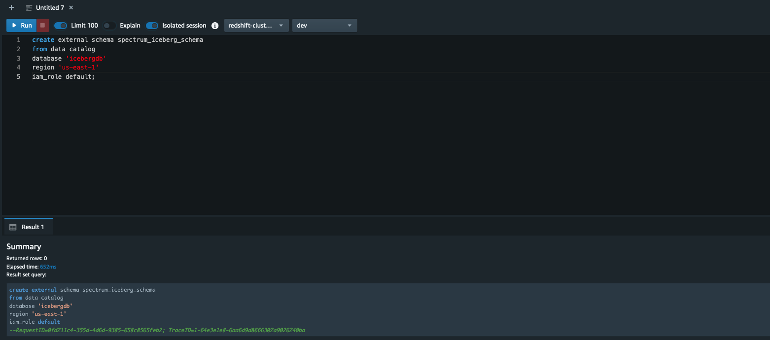
To learn about creating external schemas in Amazon Redshift, refer to create external schema
After you create the external schema spectrum\_iceberg\_schema, you can query the Iceberg table in Amazon Redshift.
Query the Iceberg table in Amazon Redshift
Run the following query in Query Editor v2. Note that spectrum\_iceberg\_schema is the name of the external schema created in Amazon Redshift and nyc\_taxi\_yellow\_iceberg is the table in the AWS Glue database used in the query:
The query data output in the following screenshot shows that the AWS Glue table with Iceberg format is queryable using Redshift Spectrum.
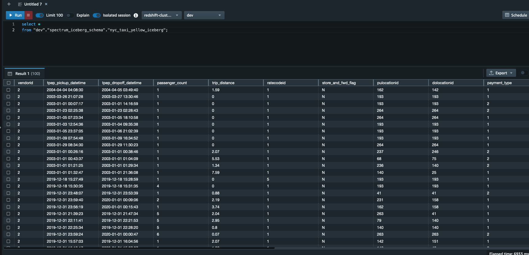
Check the explain plan of querying the Iceberg table
You can use the following query to get the explain plan output, which shows the format is ICEBERG:

Validate updates for data consistency
After the update is complete on the Iceberg table, you can query Amazon Redshift to see the transactionally consistent view of the data. Let’s run a query by picking a vendorid and for a certain pick-up and drop-off:
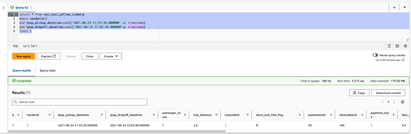
Next, update the value of passenger\_count to 4 and trip\_distance to 9.4 for a vendorid and certain pick-up and drop-off dates in Athena:
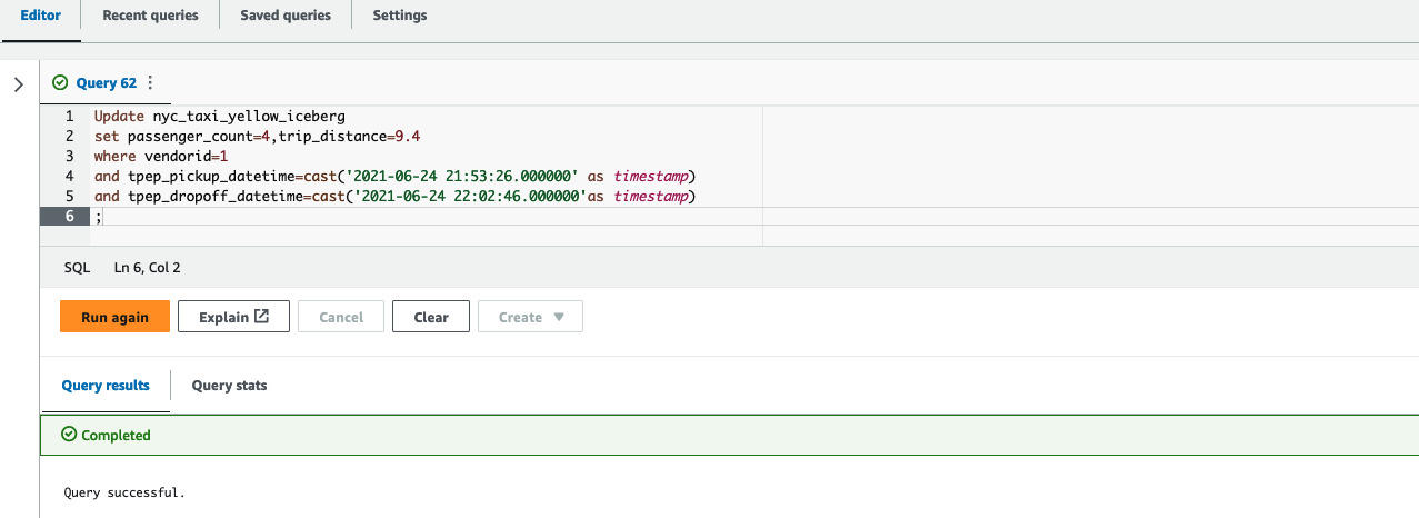
Finally, run the following query in Query Editor v2 to see the updated value of passenger\_count and trip\_distance:
As shown in the following screenshot, the update operations on the Iceberg table are available in Amazon Redshift.

Create a unified view of the local table and historical data in Amazon Redshift
As a modern data architecture strategy, you can organize historical data or less frequently accessed data in the data lake and keep frequently accessed data in the Redshift data warehouse. This provides the flexibility to manage analytics at scale and find the most cost-effective architecture solution.
In this example, we load 2 years of data in a Redshift table; the rest of the data stays on the S3 data lake because that dataset is less frequently queried.
- Use the following code to load 2 years of data in the
nyc\_taxi\_yellow\_recenttable in Amazon Redshift, sourcing from the Iceberg table:
- Next, you can remove the last 2 years of data from the Iceberg table using the following command in Athena because you loaded the data into a Redshift table in the previous step:

After you complete these steps, the Redshift table has 2 years of the data and the rest of the data is in the Iceberg table in Amazon S3.
- Create a view using the
nyc\_taxi\_yellow\_icebergIceberg table andnyc\_taxi\_yellow\_recenttable in Amazon Redshift: - Now query the view, depending on the filter conditions, Redshift Spectrum will scan either the Iceberg data, the Redshift table, or both. The following example query returns a number of records from each of the source tables by scanning both tables:

Partition evolution
Iceberg uses hidden partitioning, which means you don’t need to manually add partitions for your Apache Iceberg tables. New partition values or new partition specs (add or remove partition columns) in Apache Iceberg tables are automatically detected by Amazon Redshift and no manual operation is needed to update partitions in the table definition. The following example demonstrates this.
In our example, if the Iceberg table nyc\_taxi\_yellow\_iceberg was originally partitioned by year and later the column vendorid was added as an additional partition column, then Amazon Redshift can seamlessly query the Iceberg table nyc\_taxi\_yellow\_iceberg with two different partition schemes over a period of time.
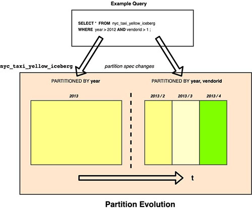
Considerations when querying Iceberg tables using Amazon Redshift
During the preview period, consider the following when using Amazon Redshift with Iceberg tables:
- Only Iceberg tables defined in the AWS Glue Data Catalog are supported.
- CREATE or ALTER external table commands are not supported, which means the Iceberg table should already exist in an AWS Glue database.
- Time travel queries are not supported.
- Iceberg versions 1 and 2 are supported. For more details on Iceberg format versions, refer to Format Versioning.
- For a list of supported data types with Iceberg tables, refer to Supported data types with Apache Iceberg tables (preview).
- Pricing for querying an Iceberg table is the same as accessing any other data formats using Amazon Redshift.
For additional details on considerations for Iceberg format tables preview, refer to Using Apache Iceberg tables with Amazon Redshift (preview).
Customer feedback
“Tinuiti, the largest independent performance marketing firm, handles large volumes of data on a daily basis and must have a robust data lake and data warehouse strategy for our market intelligence teams to store and analyze all our customer data in an easy, affordable, secure, and robust way,” says Justin Manus, Chief Technology Officer at Tinuiti. “Amazon Redshift’s support for Apache Iceberg tables in our data lake, which is the single source of truth, addresses a critical challenge in optimizing performance and accessibility and further simplifies our data integration pipelines to access all the data ingested from different sources and to power our customers’ brand potential.”
Conclusion
In this post, we showed you an example of querying an Iceberg table in Redshift using files stored in Amazon S3, cataloged as a table in the AWS Glue Data Catalog, and demonstrated some of the key features like efficient row-level update and delete, and the schema evolution experience for users to unlock the power of big data using Athena.
You can use Amazon Redshift to run queries on data lake tables in various files and table formats, such as Apache Hudi and Delta Lake, and now with Apache Iceberg (preview), which provides additional options for your modern data architectures needs.
We hope this gives you a great starting point for querying Iceberg tables in Amazon Redshift.
About the Authors
 Rohit Bansal is an Analytics Specialist Solutions Architect at AWS. He specializes in Amazon Redshift and works with customers to build next-generation analytics solutions using other AWS Analytics services.
 Satish Sathiya is a Senior Product Engineer at Amazon Redshift. He is an avid big data enthusiast who collaborates with customers around the globe to achieve success and meet their data warehousing and data lake architecture needs.
 Ranjan Burman is an Analytics Specialist Solutions Architect at AWS. He specializes in Amazon Redshift and helps customers build scalable analytical solutions. He has more than 16 years of experience in different database and data warehousing technologies. He is passionate about automating and solving customer problems with cloud solutions.
Amazon OpenSearch Serverless provides the search and analytical functionality of OpenSearch without the manual overhead of configuring, managing, and scaling OpenSearch clusters. It automatically scales the resources based on your workload, and you only pay for the resources consumed. Managing OpenSearch Serverless is simple, but with infrastructure as code (IaC) software like Terraform, you can simplify your resource management even more.
This post demonstrates how to use Terraform to create, deploy, and clean up OpenSearch Serverless infrastructure.
Solution overview
To create and deploy an OpenSearch Serverless collection with security and access policies using Terraform, you need to follow these steps:
- Initialize the Terraform configuration.
- Create an encryption policy.
- Create an OpenSearch Serverless collection.
- Create a network policy.
- Create a virtual private cloud (VPC) endpoint.
- Create a data access policy.
- Deploy using Terraform.
Prerequisites
This post assumes that you’re familiar with GitHub and Git commands.
For this walkthrough, you need the following:
- An AWS account. If you don’t have an account, you can sign up for one.
- Access to an AWS Identity and Access Management (IAM) user or role that has the minimum required permissions for setting up a collection.
- Terraform 0.12 or greater installed on your workstation. See Install Terraform.
Initialize the Terraform configuration
The sample code is available in the Terraform GitHub repo in the terraform-provider-aws/examples/opensearchserverless directory. This configuration will get you started with OpenSearch Serverless. First, clone the repository to your workstation and navigate to the directory:
$ git clone https://github.com/hashicorp/terraform-provider-aws.git && \ cd ./terraform-provider-aws/examples/opensearchserverlessInitialize the configuration to install the aws provider by running the following command:
$ terraform initThe Terraform configuration first defines the version of Terraform required and configures the AWS provider to launch resources in the Region defined by the aws\_region variable:
The variables used in this Terraform configuration are defined in the variables.tf file. This post assumes the default values are used:
Create an encryption policy
Now that the provider is installed and configured, the Terraform configuration moves on to defining OpenSearch Serverless policies for security. OpenSearch Serverless uses AWS Key Management Service (AWS KMS) to encrypt your data. The encryption is managed by an encryption policy. To create an encryption policy, use the aws\_opensearchserverless\_security\_policy resource, which has a name parameter, a type of encryption, a JSON string that defines the policy, and an optional description:
This encryption policy is named example-encryption-policy, applies to a collection named example-collection, and uses an AWS owned key to encrypt the data.
Create an OpenSearch Serverless collection
You can organize your OpenSearch indexes into a logical grouping called a collection. Create a collection using the aws\_opensearchserverless\_collection resource, which has a name parameter, and optionally, description, tags, and type:
This collection is named example-collection. If type is not specified, a time series collection is created. Supported collection types can be found in the Terraform documentation for the aws\_opensearchserverless\_collection resource. OpenSearch Serverless requires encryption at rest, so an applicable encryption policy is required before a collection can be created. The Terraform configuration explicitly defines this dependency using the depends\_on meta-argument. Errors can arise if this dependency is not defined.
Now that a collection has been created with an AWS owned KMS key, the Terraform configuration goes on to define the network and data access policy to configure access to the collection.
Create a network policy
A network policy allows access to your collection either over the public internet or through OpenSearch Serverless-managed VPC endpoints. Similar to the encryption policy, to create a network policy, use the aws\_opensearchserverless\_security\_policy resource, which has a name parameter, a type of network, a JSON string that defines the policy, and an optional description:
This network policy is named example-network-policy and applies to the collection named example-collection. This policy only allows access to the collection’s OpenSearch endpoint through a VPC endpoint, but allows public access to the OpenSearch Dashboards endpoint.
You’ll notice the VPC endpoint has not been defined yet, but it is referenced in the network policy. Terraform determines this dependency automatically and will not create the network policy until the VPC endpoint has been created.
Create a VPC endpoint
A VPC endpoint enables you to privately access your OpenSearch Serverless collection using AWS PrivateLink (for more information, refer to Access AWS services through AWS PrivateLink). Create a VPC endpoint using the aws\_opensearchserverless\_vpc\_endpoint resource, where you define name, vpc\_id, subnet\_ids , and optionally, security\_group\_ids:
Creating a VPC and all the required networking resources is out of scope for this post, but the minimum required VPC resources are created here in a separate file to demonstrate the VPC endpoint functionality. Refer to Getting Started with Amazon VPC to learn more.
Create a data access policy
The configuration defines a data source that looks up information about the context Terraform is currently running in. This data source is used when defining the data access policy. More information can be found in the Terraform documentation for aws\_caller\_identity.
A data access policy allows you to define who has access to collections and indexes. The data access policy is defined using the aws\_opensearchserverless\_access\_policy resource, which has a name parameter, a type parameter set to data, a JSON string that defines the policy, and an optional description:
This data access policy allows the current AWS role or user to perform collection-related actions on the collection named example-collection and index-related actions on the indexes in the collection.
Deploy using Terraform
Now that you have configured the necessary resources, apply the configuration using terraform apply. Before creating the resources, Terraform will describe all the resources that will be created so you can verify your configuration:
$ terraform apply...Terraform used the selected providers to generate the following execution plan. Resource actions are indicated with the following symbols: + createTerraform will perform the following actions:...Plan: 13 to add, 0 to change, 0 to destroy.Changes to Outputs: + collection\_enpdoint = (known after apply) + dashboard\_endpoint = (known after apply)Do you want to perform these actions? Terraform will perform the actions described above. Only 'yes' will be accepted to approve. Enter a value:If this is the first OpenSearch Serverless collection in your account, applying the configuration may take over 10 minutes because Terraform waits for the collection to become active.
Apply complete! Resources: 13 added, 0 changed, 0 destroyed.Outputs:collection\_enpdoint = "..."dashboard\_endpoint = "..."You have now deployed an OpenSearch Serverless time series collection with policies to configure encryption and access to the collection!
Clean up
The resources will incur costs as long as they are running, so clean up the resources when you are done using them. Use the terraform destroy command to do this:
$ terraform destroy...Terraform used the selected providers to generate the following execution plan. Resource actions are indicated with the following symbols: - destroyTerraform will perform the following actions: ...Plan: 0 to add, 0 to change, 13 to destroy.Changes to Outputs:...Do you really want to destroy all resources? Terraform will destroy all your managed infrastructure, as shown above. There is no undo. Only 'yes' will be accepted to confirm. Enter a value:Answer yes to run this plan and destroy the infrastructure.
Destroy complete! Resources: 13 destroyed.All resources created during this walkthrough have now been deleted.
Conclusion
In this post, you created an OpenSearch Serverless collection. Using IaC software like Terraform can make it simple to manage your resources like OpenSearch Serverless collections, encryption, network, and data access policies, and VPC endpoints.
Thank you to all the open-source contributors who help maintain OpenSearch and Terraform.
Try using OpenSearch Serverless with Terraform to simplify your resource management. Check out the Getting started with Amazon OpenSearch Serverless workshop and the Amazon OpenSearch Serverless Developer Guide to learn more about OpenSearch Serverless.
About the authors
 Joshua Luo is a Software Development Engineer for Amazon OpenSearch Serverless. He works on the systems that enable customers to manage and monitor their OpenSearch Serverless resources. He enjoys bouldering, photography, and videography in his free time.
 Satish Nandi is a Senior Technical Product Manager for Amazon OpenSearch Service.
Data warehousing provides a business with several benefits such as advanced business intelligence and data consistency. It plays a big role within an organization by helping to make the right strategic decision at the right moment which could have a huge impact in a competitive market. One of the major and essential parts in a data warehouse is the extract, transform, and load (ETL) process which extracts the data from different sources, applies business rules and aggregations and then makes the transformed data available for the business users.
This process is always evolving to reflect new business and technical requirements, especially when working in an ambitious market. Nowadays, more verification steps are applied to source data before processing them which so often add an administration overhead. Hence, automatic notifications are more often required in order to accelerate data ingestion, facilitate monitoring and provide accurate tracking about the process.
Amazon Redshift is a fast, fully managed, cloud data warehouse that allows you to process and run your complex SQL analytics workloads on structured and semi-structured data. It also helps you to securely access your data in operational databases, data lakes or third-party datasets with minimal movement or copying. AWS Step Functions is a fully managed service that gives you the ability to orchestrate and coordinate service components. Amazon S3 Event Notifications is an Amazon S3 feature that you can enable in order to receive notifications when specific events occur in your S3 bucket.
In this post we discuss how we can build and orchestrate in a few steps an ETL process for Amazon Redshift using Amazon S3 Event Notifications for automatic verification of source data upon arrival and notification in specific cases. And we show how to use AWS Step Functions for the orchestration of the data pipeline. It can be considered as a starting point for teams within organizations willing to create and build an event driven data pipeline from data source to data warehouse that will help in tracking each phase and in responding to failures quickly. Alternatively, you can also use Amazon Redshift auto-copy from Amazon S3 to simplify data loading from Amazon S3 into Amazon Redshift.
Solution overview
The workflow is composed of the following steps:
- A Lambda function is triggered by an S3 event whenever a source file arrives at the S3 bucket. It does the necessary verifications and then classifies the file before processing by sending it to the appropriate Amazon S3 prefix (accepted or rejected).
- There are two possibilities:
- If the file is moved to the rejected Amazon S3 prefix, an Amazon S3 event sends a message to Amazon SNS for further notification.
- If the file is moved to the accepted Amazon S3 prefix, an Amazon S3 event is triggered and sends a message with the file path to Amazon SQS.
- An Amazon EventBridge scheduled event triggers the AWS Step Functions workflow.
- The workflow executes a Lambda function that pulls out the messages from the Amazon SQS queue and generates a manifest file for the COPY command.
- Once the manifest file is generated, the workflow starts the ETL process using stored procedure.
The following image shows the workflow.

Prerequisites
Before configuring the previous solution, you can use the following AWS CloudFormation template to set up and create the infrastructure
- Give the stack a name, select a deployment VPC and define the master user for the Amazon Redshift cluster by filling in the two parameters
MasterUserNameandMasterUserPassword.
The template will create the following services:
- An S3 bucket
- An Amazon Redshift cluster composed of two ra3.xlplus nodes
- An empty AWS Step Functions workflow
- An Amazon SQS queue
- An Amazon SNS topic
- An Amazon EventBridge scheduled rule with a 5-minute rate
- Two empty AWS Lambda functions
- IAM roles and policies for the services to communicate with each other
The names of the created services are usually prefixed by the stack’s name or the word blogdemo. You can find the names of the created services in the stack’s resources tab.
Step 1: Configure Amazon S3 Event Notifications
Create the following four folders in the S3 bucket:
- received
- rejected
- accepted
- manifest
In this scenario, we will create the following three Amazon S3 event notifications:
- Trigger an AWS Lambda function on the received folder.
- Send a message to the Amazon SNS topic on the rejected folder.
- Send a message to Amazon SQS on the accepted folder.
To create an Amazon S3 event notification:
- Go to the bucket’s Properties tab.
- In the Event Notifications section, select Create Event Notification.
- Fill in the necessary properties:
- Give the event a name.
- Specify the appropriate prefix or folder (
accepted/,rejected/orreceived/). - Select All object create events as an event type.
- Select and choose the destination (AWS lambda, Amazon SNS or Amazon SQS).
Note: for an AWS Lambda destination, choose the function that starts with${stackname}-blogdemoVerify\_%
At the end, you should have three Amazon S3 events:
- An event for the received prefix with an AWS Lambda function as a destination type.
- An event for the accepted prefix with an Amazon SQS queue as a destination type.
- An event for the rejected prefix with an Amazon SNS topic as a destination type.
The following image shows what you should have after creating the three Amazon S3 events:

Step 2: Create objects in Amazon Redshift
Connect to the Amazon Redshift cluster and create the following objects:
- Three schemas:
- A table in the
blogdemo\_stagingandblogdemo\_coreschemas: - A stored procedure to extract and load data into the target schema:
- Set the role
${stackname}-blogdemoRoleRedshift\_%as a default role:- In the Amazon Redshift console, go to clusters and click on the cluster
blogdemoRedshift%. - Go to the Properties tab.
- In the Cluster permissions section, select the role
${stackname}-blogdemoRoleRedshift%. - Click on Set default then Make default.
- In the Amazon Redshift console, go to clusters and click on the cluster
Step 3: Configure Amazon SQS queue
The Amazon SQS queue can be used as it is; this means with the default values. The only thing you need to do for this demo is to go to the created queue ${stackname}-blogdemoSQS% and purge the test messages generated (if any) by the Amazon S3 event configuration. Copy its URL in a text file for further use (more precisely, in one of the AWS Lambda functions).
Step 4: Setup Amazon SNS topic
- In the Amazon SNS console, go to the topic
${stackname}-blogdemoSNS% - Click on the Create subscription button.
- Choose the
blogdemotopic ARN, email protocol, type your email and then click on Create subscription. - Confirm your subscription in your email that you received.

Step 5: Customize the AWS Lambda functions
- The following code verifies the name of a file. If it respects the naming convention, it will move it to the accepted folder. If it does not respect the naming convention, it will move it to the rejected one. Copy it to the AWS Lambda function
${stackname}-blogdemoLambdaVerifyand then deploy it: - The second AWS Lambda function
${stackname}-blogdemonLambdaGenerate%retrieves the messages from the Amazon SQS queue and generates and stores a manifest file in the S3 bucket manifest folder. Copy the following content, replace the variable${sqs\_url}by the value retrieved in Step 3 and then click on Deploy.
Step 6: Add tasks to the AWS Step Functions workflow
Create the following workflow in the state machine ${stackname}-blogdemoStepFunctions%.

If you would like to accelerate this step, you can drag and drop the content of the following JSON file in the definition part when you click on Edit. Make sure to replace the three variables:
${GenerateManifestFileFunctionName}by the${stackname}-blogdemoLambdaGenerate%arn.${RedshiftClusterIdentifier}by the Amazon Redshift cluster identifier.${MasterUserName}by the username that you defined while deploying the CloudFormation template.

Step 7: Enable Amazon EventBridge rule
Enable the rule and add the AWS Step Functions workflow as a rule target:
- Go to the Amazon EventBridge console.
- Select the rule created by the Amazon CloudFormation template and click on Edit.
- Enable the rule and click Next.
- You can change the rate if you want. Then select Next.
- Add the AWS Step Functions state machine created by the CloudFormation template
blogdemoStepFunctions%as a target and use an existing role created by the CloudFormation template${stackname}-blogdemoRoleEventBridge%

- Click on Next and then Update rule.
Test the solution
In order to test the solution, the only thing you should do is upload some csv files in the received prefix of the S3 bucket. Here are some sample data; each file contains 1000 rows of rideshare data.
If you upload them in one click, you should receive an email because the ridesharedata2022.csv does not respect the naming convention. The other three files will be loaded in the target table blogdemo\_core.rideshare. You can check the Step Functions workflow to verify that the process finished successfully.

Clean up
- Go to the Amazon EventBridge console and delete the rule
${stackname}-blogdemoevenbridge%. - In the Amazon S3 console, select the bucket created by the CloudFormation template
${stackname}-blogdemobucket%and click on Empty. - Go to Subscriptions in the Amazon SNS console and delete the subscription created in Step 4.
- In the AWS CloudFormation console, select the stack and delete it.
Conclusion
In this post, we showed how different AWS services can be easily implemented together in order to create an event-driven architecture and automate its data pipeline, which targets the cloud data warehouse Amazon Redshift for business intelligence applications and complex queries.
About the Author
 Ziad WALI is an Acceleration Lab Solutions Architect at Amazon Web Services. He has over 10 years of experience in databases and data warehousing where he enjoys building reliable, scalable and efficient solutions. Outside of work, he enjoys sports and spending time in nature.
To improve a Spark application's efficiency, it’s essential to monitor its performance and behavior. In this post, we demonstrate how to publish detailed Spark metrics from Amazon EMR to Amazon CloudWatch. This will give you the ability to identify bottlenecks while optimizing resource utilization.
Amazon OpenSearch Serverless is a serverless deployment option for Amazon OpenSearch Service that makes it simple for you to run search and analytics workloads without having to think about infrastructure management. The compute capacity used for data ingestion, and search and query in OpenSearch Serverless is measured in OpenSearch Compute Units (OCUs). Customers can configure […]
Amazon Security Lake centralizes access and management of your security data by aggregating security event logs from AWS environments, other cloud providers, on premise infrastructure, and other software as a service (SaaS) solutions. By converting logs and events using Open Cybersecurity Schema Framework, an open standard for storing security events in a common and shareable format, […]
Since its release in January 2021, the OpenSearch project has released 14 versions through June 2023. Amazon OpenSearch Service supports the latest versions of OpenSearch up to version 2.7. OpenSearch Service provides two configuration options to deploy and operate OpenSearch at scale in the cloud. With OpenSearch Service managed domains, you specify a hardware configuration […]
The post Archive and Purge Data for Amazon RDS for PostgreSQL and Amazon Aurora with PostgreSQL Compatibility using pg_partman and Amazon S3 proposes data archival as a critical part of data management and shows how to efficiently use PostgreSQL’s native range partition to partition current (hot) data with pg_partman and archive historical (cold) data in […]
In this post, we explore how to deploy Amazon CloudWatch metrics using an AWS CloudFormation template to monitor an OpenSearch Service domain’s storage and shard skew. This solution uses an AWS Lambda function to extract storage and shard distribution metadata from your OpenSearch Service domain, calculates the level of skew, and then pushes this information to CloudWatch metrics so that you can easily monitor, alert, and respond.
Amazon OpenSearch Service has long supported both lexical and vector search, since the introduction of its kNN plugin in 2020. With recent developments in generative AI, including AWS’s launch of Amazon Bedrock earlier in 2023, you can now use Amazon Bedrock-hosted models in conjunction with the vector database capabilities of OpenSearch Service, allowing you to implement semantic search, retrieval augmented generation (RAG), recommendation engines, and rich media search based on high-quality vector search. The recent launch of the vector engine for Amazon OpenSearch Serverless makes it even easier to deploy such solutions.
We recently announced new enhancements to Amazon OpenSearch Serverless that can scan and search source data sizes of up to 6 TB. At launch, OpenSearch Serverless supported searching one or more indexes within a collection, with the total combined size of up to 1 TB. With the support for 6 TB source data, you can now scale up your log analytics, machine learning applications, and ecommerce data more effectively. With OpenSearch Serverless, you can enjoy the benefits of these expanded limits without having to worry about sizing, monitoring your usage, or manually scaling an OpenSearch domain.
Apache Iceberg is an open table format for large datasets in Amazon Simple Storage Service (Amazon S3) and provides fast query performance over large tables, atomic commits, concurrent writes, and SQL-compatible table evolution. Iceberg has become very popular for its support for ACID transactions in data lakes and features like schema and partition evolution, time […]
Apache Iceberg is an open table format for very large analytic datasets. Iceberg manages large collections of files as tables, and it supports modern analytical data lake operations such as record-level insert, update, delete, and time travel queries. The Iceberg specification allows seamless table evolution such as schema and partition evolution, and its design is […]
Automated Data Analytics (ADA) on AWS is an AWS solution that enables you to derive meaningful insights from data in a matter of minutes through a simple and intuitive user interface. ADA offers an AWS-native data analytics platform that is ready to use out of the box by data analysts for a variety of use […]
As customers accelerate their migrations to the cloud and transform their businesses, some find themselves in situations where they have to manage data analytics in a multi-cloud environment, such as acquiring a company that runs on a different cloud provider. Customers who use multi-cloud environments often face challenges in data access and compatibility that can […]
This post is the first in a series dedicated to the art and science of practical data mesh implementation (for an overview of data mesh, read the original whitepaper The data mesh shift). The series attempts to bridge the gap between the tenets of data mesh and its real-life implementation by deep-diving into the functional […]
This post is written in collaboration with Elijah Ball from Ontraport. Customers are implementing data and analytics workloads in the AWS Cloud to optimize cost. When implementing data processing workloads in AWS, you have the option to use technologies like Amazon EMR or serverless technologies like AWS Glue. Both options minimize the undifferentiated heavy lifting […]
Amazon Managed Workflows for Apache Airflow (Amazon MWAA) is a managed orchestration service for Apache Airflow that makes it simple to set up and operate end-to-end data pipelines in the cloud. Trusted across various industries, Amazon MWAA helps organizations like Siemens, ENGIE, and Choice Hotels International enhance and scale their business workflows, while significantly improving security […]
Building a streaming data solution requires thorough testing at the scale it will operate in a production environment. Streaming applications operating at scale often handle large volumes of up to GBs per second, and it’s challenging for developers to simulate high-traffic Amazon Kinesis-based applications to generate such load easily. Amazon Kinesis Data Streams and Amazon […]
AWS serverless services, including but not limited to AWS Lambda, AWS Glue, AWS Fargate, Amazon EventBridge, Amazon Athena, Amazon Simple Notification Service (Amazon SNS), Amazon Simple Queue Service (Amazon SQS), and Amazon Simple Storage Service (Amazon S3), have become the building blocks for any serverless data lake, providing key mechanisms to ingest and transform data […]
Modern applications apply security controls across many systems and their subsystems. Keeping all of these systems in sync would be a major undertaking if you tried to implement it separately. Centralized identity management is the way to maintain a single identity provider (IdP) that can authenticate actors and manage and distribute their rights. OpenSearch is […]
Amazon Redshift is a fully managed, petabyte-scale data warehouse service in the cloud. Tens of thousands of customers use Amazon Redshift to process exabytes of data every day to power their analytics workloads. Many businesses use different software tools to analyze historical data and past patterns to forecast future demand and trends to make more […]
Today’s modern data lakes span multiple accounts, AWS Regions, and lines of business in organizations. Companies also have employees and do business across multiple geographic regions and even around the world. It’s important that their data solution gives them the ability to share and access data securely and safely across Regions. The AWS Glue Data […]
We recently announced support for streaming extract, transform, and load (ETL) jobs in AWS Glue version 4.0, a new version of AWS Glue that accelerates data integration workloads in AWS. AWS Glue streaming ETL jobs continuously consume data from streaming sources, clean and transform the data in-flight, and make it available for analysis in seconds. AWS also offers a broad selection of services to support your needs. A database replication service such as AWS Database Migration Service (AWS DMS) can replicate the data from your source systems to Amazon Simple Storage Service (Amazon S3), which commonly hosts the storage layer of the data lake. This post demonstrates how to apply CDC changes from Amazon Relational Database Service (Amazon RDS) or other relational databases to an S3 data lake, with flexibility to denormalize, transform, and enrich the data in near-real time.
Today, more than 400 organizations have signed The Climate Pledge, a commitment to reach net-zero carbon by 2040. Some of the drivers that lead to setting explicit climate goals include customer demand, current and anticipated government relations, employee demand, investor demand, and sustainability as a competitive advantage. AWS customers are increasingly interested in ways to […]
This post was co-written by Sheel Saket, Senior Data Science Manager at FIS, and Rupesh Tiwari, Senior Architect at Amazon Web Services. Do you ever find yourself grappling with multiple defect logging mechanisms, scattered project management tools, and fragmented software development platforms? Have you experienced the frustration of lacking a unified view, hindering your ability […]
Amazon Kinesis Data Streams is a serverless data streaming service that makes it easy to capture, process, and store streaming data at any scale. As customers collect and stream more types of data, they have asked for simpler, elastic data streams that can handle variable and unpredictable data traffic. In November 2021, Amazon Web Services […]
In the world of software engineering and development, organizations use project management tools like Atlassian Jira Cloud. Managing projects with Jira leads to rich datasets, which can provide historical and predictive insights about project and development efforts. Although Jira Cloud provides reporting capability, loading this data into a data lake will facilitate enrichment with other […]
Data has become an integral part of most companies, and the complexity of data processing is increasing rapidly with the exponential growth in the amount and variety of data. Data engineering teams are faced with the following challenges: Manipulating data to make it consumable by business users Building and improving extract, transform, and load (ETL) […]
Apache Flink and Apache Spark are both open-source, distributed data processing frameworks used widely for big data processing and analytics. Spark is known for its ease of use, high-level APIs, and the ability to process large amounts of data. Flink shines in its ability to handle processing of data streams in real-time and low-latency stateful […]
Amazon Athena is a serverless, interactive analytics service built on the Trino, PrestoDB, and Apache Spark open-source frameworks. You can use Athena to run SQL queries on petabytes of data stored on Amazon Simple Storage Service (Amazon S3) in widely used formats such as Parquet and open-table formats like Apache Iceberg, Apache Hudi, and Delta […]
Amazon Redshift is a petabyte-scale, enterprise-grade cloud data warehouse service delivering the best price-performance. Today, tens of thousands of customers run business-critical workloads on Amazon Redshift to cost-effectively and quickly analyze their data using standard SQL and existing business intelligence (BI) tools. Amazon Redshift now makes it easier for you to run queries in AWS […]
The GDPR (General Data Protection Regulation) right to be forgotten, also known as the right to erasure, gives individuals the right to request the deletion of their personally identifiable information (PII) data held by organizations. This means that individuals can ask companies to erase their personal data from their systems and any third parties with […]
AWS Glue Studio is now integrated with AWS Glue DataBrew. AWS Glue Studio is a graphical interface that makes it easy to create, run, and monitor extract, transform, and load (ETL) jobs in AWS Glue. DataBrew is a visual data preparation tool that enables you to clean and normalize data without writing any code. The […]
Amazon Redshift is a widely used, fully managed, petabyte-scale cloud data warehouse. Tens of thousands of customers use Amazon Redshift to process exabytes of data every day to power their analytics workloads. With the launch of Amazon Redshift Serverless and the various deployment options Amazon Redshift provides (such as instance types and cluster sizes), customers […]
Amazon Redshift is a fully managed, scalable cloud data warehouse that accelerates your time to insights with fast, easy, and secure analytics at scale. Tens of thousands of customers rely on Amazon Redshift to analyze exabytes of data and run complex analytical queries, making it the widely used cloud data warehouse. You can run and […]
Amazon EMR is the cloud big data solution for petabyte-scale data processing, interactive analytics, and machine learning using open-source frameworks such as Apache Spark, Apache Hive, and Presto. Customers asked us for features that would further improve the resiliency and scalability of their Amazon EMR on EC2 clusters, including their large, long-running clusters. We have […]
Data is a key enabler for your business. Many AWS customers have integrated their data across multiple data sources using AWS Glue, a serverless data integration service, in order to make data-driven business decisions. To grow the power of data at scale for the long term, it’s highly recommended to design an end-to-end development lifecycle […]
Data is essential for businesses to make informed decisions, improve operations, and innovate. Integrating data from different sources can be a complex and time-consuming process. AWS offers AWS Glue to help you integrate your data from multiple sources on serverless infrastructure for analysis, machine learning (ML), and application development. AWS Glue provides different authoring experiences […]
We are pleased to announce the preview release of the vector engine for Amazon OpenSearch Serverless. The vector engine provides a simple, scalable, and high-performing similarity search capability in Amazon OpenSearch Serverless that makes it easy for you to build modern machine learning (ML) augmented search experiences and generative artificial intelligence (AI) applications without having […]
This is a guest blog post co-written with Zack Rossman from Alcion. Alcion, a security-first, AI-driven backup-as-a-service (BaaS) platform, helps Microsoft 365 administrators quickly and intuitively protect data from cyber threats and accidental data loss. In the event of data loss, Alcion customers need to search metadata for the backed-up items (files, emails, contacts, events, […]
Amazon Redshift Serverless makes it simple to run and scale analytics in seconds. It automatically provisions and intelligently scales data warehouse compute capacity to deliver fast performance, and you pay only for what you use. Just load your data and start querying right away in the Amazon Redshift Query Editor or in your favorite business […]
This is a guest post co-written with Cameron Davie from Talend. Today, in order to accelerate and scale data analytics, companies are looking for an approach to minimize infrastructure management and predict computing needs for different types of workloads, including spikes and ad hoc analytics. The integration of Talend Cloud and Talend Stitch with Amazon […]
Data-driven organizations treat data as an asset and use it across different lines of business (LOBs) to drive timely insights and better business decisions. Many organizations have a distributed tools and infrastructure across various business units. This leads to having data across many instances of data warehouses and data lakes using a modern data architecture […]
Apache Hive is a SQL-based data warehouse system for processing highly distributed datasets on the Apache Hadoop platform. There are two key components to Apache Hive: the Hive SQL query engine and the Hive metastore (HMS). The Hive metastore is a repository of metadata about the SQL tables, such as database names, table names, schema, […]
This post is co-written with Eliad Gat and Oded Lifshiz from Orca Security. With data becoming the driving force behind many industries today, having a modern data architecture is pivotal for organizations to be successful. One key component that plays a central role in modern data architectures is the data lake, which allows organizations to […]
Amazon Redshift is a fully managed and petabyte-scale cloud data warehouse that is used by tens of thousands of customers to process exabytes of data every day to power their analytics workload. You can structure your data, measure business processes, and get valuable insights quickly can be done by using a dimensional model. Amazon Redshift […]
Today, we are pleased to announce a new AWS Glue connector for Google Cloud Storage that allows you to move data bi-directionally between Google Cloud Storage and Amazon Simple Storage Service (Amazon S3). We’ve seen that there is a demand to design applications that enable data to be portable across cloud environments and give you […]
Customers use Amazon Managed Workflows for Apache Airflow (Amazon MWAA) to run Apache Airflow at scale in the cloud. They want to use their existing login solutions developed using OpenID Connect (OIDC) providers with Amazon MWAA; this allows them to provide a uniform authentication and single sign-on (SSO) experience using their adopted identity providers (IdP) […]
Color plays a crucial role in visualizations. It conveys meaning, captures attention, and enhances aesthetics. You can quickly grasp important information when key insights and data points pop with color. However, it’s important to use color judiciously to enhance readability and ensure correct interpretation. Color should also be accessible and consistent to enable users to […]
In this post, we show how to build a log ingestion pipeline using the new Amazon OpenSearch Ingestion, a fully managed data collector that delivers real-time log and trace data to Amazon OpenSearch Service domains. OpenSearch Ingestion is powered by the open-source data collector Data Prepper. Data Prepper is part of the open-source OpenSearch project. […]
The technology landscape has been evolving rapidly, with waves of change impacting IT from every angle. It is causing a ripple effect across IT organizations and shifting the way IT delivers applications and services. The change factors impacting IT organizations include: The shift from a traditional application model to a services-based application model (SaaS, PaaS) […]
Amazon Finance Automation (FinAuto) is the tech organization of Amazon Finance Operations (FinOps). Its mission is to enable FinOps to support the growth and expansion of Amazon businesses. It works as a force multiplier through automation and self-service, while providing accurate and on-time payments and collections. FinAuto has a unique position to look across FinOps […]
AWS customers are looking for an efficient tracking method of support cases raised with AWS Support across their multiple interconnected accounts. Having a unified view lets the cloud operations team derive actionable insights across the support cases raised by different business units and accounts. This helps ensure that the team has a comprehensive understanding of […]
This is a guest post co-authored by Jacques Steyn, Senior Manager Professional Services at Altron Group. Altron is a pioneer of providing data-driven solutions for their customers by combining technical expertise with in-depth customer understanding to provide highly differentiated technology solutions. Alongside their partner AWS, they participated in AWS Data-Driven Everything (D2E) workshops and a […]
This is a guest post authored by Kris Bliesner and Mike Brown from Vega Cloud. Vega Cloud is a premier member of the FinOps Foundation, a program by Linux Foundation supporting FinOps practitioners on cloud financial management best practices. Vega Cloud provides a place where finance, engineers, and innovators come together to accelerate the business […]
This blog post is co-written with Zygimantas Koncius from Etleap. Organizations use their data to extract valuable insights and drive informed business decisions. With a wide array of data sources, including transactional databases, log files, and event streams, you need a simple-to-use solution capable of efficiently ingesting and transforming large volumes of data in real […]
Using embedded analytics from Amazon QuickSight can simplify the process of equipping your application with functional visualizations without any complex development. There are multiple ways to embed QuickSight dashboards into application. In this post, we look at how it can be done using React and the Amazon QuickSight Embedding SDK. Dashboard consumers often don’t have […]
This is a guest post by Gonzalo Lezma from Amazon Mexico FP&A. The Financial Planning and Analysis (FP&A) team in Mexico provides strategic support to Amazon’s CFO and executive team on planning, analysis, and reporting related to Amazon Mexico. We produce and manage key finance deliverables, such as internal profit and loss (P&L) reports for […]
Amazon OpenSearch Serverless helps you index, analyze, and search your logs and data using OpenSearch APIs and dashboards. The OpenSearch Serverless collection is a group of indexes. API and dashboard clients can access the collections from public networks or one or more VPCs. For VPC access to collections and dashboards, you can create VPC endpoints. […]
Extracting time series on given geographical coordinates from satellite or Numerical Weather Prediction data can be challenging because of the volume of data and of its multidimensional nature (time, latitude, longitude, height, multiple parameters). This type of processing can be found in weather and climate research, but also in applications like photovoltaic and wind power. […]
Backtesting is a process used in quantitative finance to evaluate trading strategies using historical data. This helps traders determine the potential profitability of a strategy and identify any risks associated with it, enabling them to optimize it for better performance. Index rebalancing arbitrage takes advantage of short-term price discrepancies resulting from ETF managers’ efforts to […]
This is a guest post by Vinod Nambiar from Position2. Position2 is a leading US-based growth marketing services provider focused on data-driven strategy and technology to deliver growth with improved return on investment (ROI). Position2 was established in 2006 in Silicon Valley and has a clientele spanning American Express, Lenovo, Fujitsu, and Thales. We work […]
Amazon Kinesis Data Analytics makes it easy to transform and analyze streaming data in real time. In this post, we discuss why AWS recommends moving from Kinesis Data Analytics for SQL Applications to Amazon Kinesis Data Analytics for Apache Flink to take advantage of Apache Flink’s advanced streaming capabilities. We also show how to use […]
Amazon Redshift is a fully managed, petabyte-scale data warehouse service in the cloud that delivers powerful and secure insights on all your data with the best price-performance. With Amazon Redshift, you can analyze your data to derive holistic insights about your business and your customers. In many organizations, one or multiple Amazon Redshift data warehouses […]
Amazon Aurora zero-ETL integration with Amazon Redshift was announced at AWS re:Invent 2022 and is now available in public preview for Amazon Aurora MySQL-Compatible Edition 3 (compatible with MySQL 8.0) in regions us-east-1, us-east-2, us-west-2, ap-northeast-1 and eu-west-1. For more details, refer to the What’s New Post. In this post, we provide step-by-step guidance on […]
Data is at the center of every application, process, and business decision. When data is used to improve customer experiences and drive innovation, it can lead to business growth. According to Forrester, advanced insights-driven businesses are 8.5 times more likely than beginners to report at least 20% revenue growth. However, to realize this growth, managing […]
This is a guest post by Jon Walker and Ari Orlinsky from iostudio written in collaboration with Sumitha AP from AWS. iostudio is an award-winning marketing agency based in Nashville, TN. We build solutions that bring brands to life, making content and platforms work together. We serve our customers, who range from small technology startups […]
In today’s digital world, data is generated by a large number of disparate sources and growing at an exponential rate. Companies are faced with the daunting task of ingesting all this data, cleansing it, and using it to provide outstanding customer experience. Typically, companies ingest data from multiple sources into their data lake to derive […]
This blog post is co-written with Ori Nakar from Imperva. Imperva Cloud WAF protects hundreds of thousands of websites and blocks billions of security events every day. Events and many other security data types are stored in Imperva’s Threat Research Multi-Region data lake. Imperva harnesses data to improve their business outcomes. To enable this transformation […]
AWS Glue interactive sessions allow engineers to build, test, and run data preparation and analytics workloads in an interactive notebook. Interactive sessions provide isolated development environments, take care of the underlying compute cluster, and allow for configuration to stop idling resources. Glue interactive sessions provides default recommended configurations, and also allows users to customize the […]
Large organizations processing huge volumes of data usually store it in Amazon Simple Storage Service (Amazon S3) and query the data to make data-driven business decisions using distributed analytics engines such as Amazon Athena. If you simply run queries without considering the optimal data layout on Amazon S3, it results in a high volume of […]
OpenSearch is a scalable, flexible, and extensible open-source software suite for search, analytics, security monitoring, and observability applications, licensed under the Apache 2.0 license. It comprises a search engine, OpenSearch, which delivers low-latency search and aggregations, OpenSearch Dashboards, a visualization and dashboarding tool, and a suite of plugins that provide advanced capabilities like alerting, fine-grained […]
Amazon Redshift is a fast, petabyte-scale cloud data warehouse that makes it simple and cost-effective to analyze all of your data using standard SQL. Tens of thousands of customers today rely on Amazon Redshift to analyze exabytes of data and run complex analytical queries, making it the most widely used cloud data warehouse. You can […]
Amazon DynamoDB is a fully managed NoSQL service that delivers single-digit millisecond performance at any scale. It’s used by thousands of customers for mission-critical workloads. Typical use cases for DynamoDB are an ecommerce application handling a high volume of transactions, or a gaming application that needs to maintain scorecards for players and games. In traditional […]
It’s common to store the logs generated by customer’s applications and services in various tools. These logs are important for compliance, audits, troubleshooting, security incident responses, meeting security policies, and many other purposes. You can perform log analysis on these logs to understand users’ application behavior and patterns to make informed decisions. When running workloads […]
Amazon Athena is an interactive query service that makes it easy to analyze data in Amazon Simple Storage Service (Amazon S3) and data sources residing in AWS, on-premises, or other cloud systems using SQL or Python. Athena is built on open-source Trino and Presto engines, and Apache Spark frameworks, with no provisioning or configuration effort […]
With Amazon Managed Streaming for Apache Kafka (Amazon MSK), you can build and run applications that use Apache Kafka to process streaming data. To process streaming data, organizations either use multiple Kafka clusters based on their application groupings, usage scenarios, compliance requirements, and other factors, or a dedicated Kafka cluster for the entire organization. It […]
Kafka quotas are integral to multi-tenant Kafka clusters. They prevent Kafka cluster performance from being negatively affected by poorly behaved applications overconsuming cluster resources. Furthermore, they enable the central streaming data platform to be operated as a multi-tenant platform and used by downstream and upstream applications across multiple business lines. Kafka supports two types of quotas: […]
With the recent introduction of Amazon Security Lake, it has never been simpler to access all your security-related data in one place. Whether it’s findings from AWS Security Hub, DNS query data from Amazon Route 53, network events such as VPC Flow Logs, or third-party integrations provided by partners such as Barracuda Email Protection, Cisco […]
Amazon QuickSight powers data-driven organizations with unified business intelligence (BI) at hyperscale. With QuickSight, all users can meet varying analytic needs from the same source of truth through modern interactive dashboards, paginated reports, embedded analytics and natural language queries. We have introduced dataset parameters, a new kind of parameter in QuickSight that can help you […]
In this post, we explain how you can enable business users to ask and answer questions about data using their everyday business language by using the Amazon QuickSight natural language query function, Amazon QuickSight Q. QuickSight is a unified BI service providing modern interactive dashboards, natural language querying, paginated reports, machine learning (ML) insights, and […]
In today’s world, customers manage vast amounts of data in their Amazon Simple Storage Service (Amazon S3) data lakes, which requires convoluted data pipelines to continuously understand the changes in the data layout and make them available to consuming systems. AWS Glue crawlers provide a straightforward way to catalog data in the AWS Glue Data […]
In this post, we show how you can use AWS Clean Rooms to enable data collaboration between public health agencies. Public health governmental agencies need to understand trends related to a variety of health conditions and care across populations in order to create policies and treatments with the goal of improving the well-being of the […]
Organizations use data from many sources to understand, analyze, and grow their business. These data sources are often spread across various public cloud providers. Enterprises may also expand their footprint by mergers and acquisitions, and during such events they often end up with data spread across different public cloud providers. These scenarios can create the […]
Amazon OpenSearch Service is a managed service that makes it simple to secure, deploy, and operate OpenSearch clusters at scale in the AWS Cloud. Last year, we introduced Shard Indexing Backpressure and admission control, which monitors cluster resources and incoming traffic to selectively reject requests that would otherwise pose stability risks like out of memory […]
The AWS Professional Services (ProServe) Insights team builds global operational data products that serve over 8,000 users within Amazon. Our team was formed in 2019 as an informal group of four analysts who supported ad hoc analysis for a division of ProServe consultants. ProServe is responsible for assisting enterprises as they shift to the cloud […]
In the second post of the series, we discussed some core concepts of the Amazon Managed Streaming for Apache Kafka (Amazon MSK) tiered storage feature and explained how read and write operations work in a tiered storage enabled cluster. This post focuses on how to properly size your MSK tiered storage cluster, which metrics to […]
This is a joint post co-authored with Nir Tsruya from Klarna Bank AB. Klarna is a leading global payments and shopping service, providing smarter and more flexible shopping and purchase experiences to 150 million active consumers across more than 500,000 merchants in 45 countries. Klarna offers direct payments, pay after delivery options, and instalment plans […]
Amazon QuickSight is a scalable, serverless, embeddable, machine learning (ML) powered business intelligence (BI) service built for the cloud that supports identity federation in both Standard and Enterprise editions. Organizations are working toward centralizing their identity and access strategy across all their applications, including on-premises and third-party. Many organizations use Keycloak as their identity provider […]
Amazon QuickSight is a scalable, serverless, machine learning (ML)-powered business intelligence (BI) solution that makes it simple to connect to your data, create interactive dashboards, get access to ML-enabled insights, enable natural language querying of your data, and share visuals and dashboards with tens of thousands of internal and external users, either within QuickSight itself […]
This is a guest post by Tony McCormack from Joulica. Joulica is an Ireland-based startup in the contact center industry. Our founders previously led contact center research and development for a global contact center technology provider, and we founded Joulica because we saw that the shift to the cloud and growing demand for data and […]
Organizations across the world are increasingly relying on streaming data, and there is a growing need for real-time data analytics, considering the growing velocity and volume of data being collected. This data can come from a diverse range of sources, including Internet of Things (IoT) devices, user applications, and logging and telemetry information from applications, […]
Amazon EMR is the industry-leading cloud big data solution, providing a collection of open-source frameworks such as Spark, Hive, Hudi, and Presto, fully managed and with per-second billing. Amazon EMR on Amazon EKS is a deployment option allowing you to deploy Amazon EMR on the same Amazon Elastic Kubernetes Service (Amazon EKS) clusters that is […]
A modern data architecture enables companies to ingest virtually any type of data through automated pipelines into a data lake, which provides highly durable and cost-effective object storage at petabyte or exabyte scale. This data is then projected into analytics services such as data warehouses, search systems, stream processors, query editors, notebooks, and machine learning […]
In today’s fast-paced digital world, businesses rely heavily on their data to make informed decisions. This data is often stored and analyzed using various tools, such as Amazon OpenSearch Service, a powerful search and analytics service offered by AWS. OpenSearch Service provides real-time insights into your data to support use cases like interactive log analytics, […]
Business intelligence (BI) and IT operations (BIOps) teams often need to automate and accelerate the deployment of BI assets to ensure business continuity. We heard that you wanted an automated and scalable way to deploy, back up, and replicate Amazon QuickSight assets at scale so that BIOps teams within your organization can work in an […]
This is a guest blog post co-written with Sumesh M R from Cargotec and Tero Karttunen from Knowit Finland. Cargotec (Nasdaq Helsinki: CGCBV) is a Finnish company that specializes in cargo handling solutions and services. They are headquartered in Helsinki, Finland, and operates globally in over 100 countries. With its leading cargo handling solutions and […]
Amazon EMR on EKS provides a deployment option for Amazon EMR that allows organizations to run open-source big data frameworks on Amazon Elastic Kubernetes Service (Amazon EKS). With EMR on EKS, Spark applications run on the Amazon EMR runtime for Apache Spark. This performance-optimized runtime offered by Amazon EMR makes your Spark jobs run fast […]
We are excited to announce the General Availability of AWS Glue Data Quality.
Our journey started by working backward from our customers who create, manage, and operate data lakes and data warehouses for analytics and machine learning. To make confident business decisions, the underlying data needs to be accurate and recent. Otherwise, data consumers lose trust in the data and make suboptimal or incorrect decisions. For example, medical researchers found that across 79,000 emergency department encounters of pediatric patients in a hospital, incorrect or missing patient weight measurements led to medication dosing errors in 34% of cases. A data quality check to identify missing patient weight measurements or a check to ensure patients’ weights are trending within certain thresholds would have alerted respective teams to identify these discrepancies.
For our customers, setting up these data quality checks is manual, time consuming, and error prone. It takes days for data engineers to identify and implement data quality rules. They have to gather detailed data statistics, such as minimums, maximums, averages, and correlations. They have to then review the data statistics to identify data quality rules, and write code to implement these checks in their data pipelines. Data engineers must then write code to monitor data pipelines, visualize quality scores, and alert them when anomalies occur. They have to repeat these processes across thousands of datasets and the hundreds of data pipelines populating them. Some customers adopt commercial data quality solutions; however, these solutions require time-consuming infrastructure management and are expensive. Our customers needed a simple, cost-effective, and automatic way to manage data quality.
In this post, we discuss the capabilities and features of AWS Glue Data Quality.
Capabilities of AWS Glue Data Quality
AWS Glue Data Quality accelerates your data quality journey with the following key capabilities:
- Serverless – AWS Glue Data Quality is a feature of AWS Glue, which eliminates the need for infrastructure management, patching, and maintenance.
- Reduced manual efforts with recommending data quality rules and out-of-the-box rules – AWS Glue Data Quality computes data statistics such as minimums, maximums, histograms, and correlations for datasets. It then uses these statistics to automatically recommend data quality rules that check for data freshness, accuracy, and integrity. This reduces manual data analysis and rule identification efforts from days to hours. You can then augment recommendations with out-of-the-box data quality rules. The following table lists the rules that are supported by AWS Glue Data Quality as of writing. For an up-to-date list, refer to Data Quality Definition Language (DQDL).
| Rule Type | Description |
AggregateMatch | Checks if two datasets match by comparing summary metrics like total sales amount. Useful for customers to compare if all data is ingested from source systems. |
ColumnCorrelation | Checks how well two columns are corelated. |
ColumnCount | Checks if any columns are dropped. |
ColumnDataType | Checks if a column is compliant with a data type. |
ColumnExists | Checks if columns exist in a dataset. This allows customers building self-service data platforms to ensure certain columns are made available. |
ColumnLength | Checks if length of data is consistent. |
ColumnNamesMatchPattern | Checks if column names match defined patterns. Useful for governance teams to enforce column name consistency. |
ColumnValues | Checks if data is consistent per defined values. This rule supports regular expressions. |
Completeness | Checks for any blank or NULLs in data. |
CustomSql | Customers can implement almost any type of data quality checks in SQL. |
DataFreshness | Checks if data is fresh. |
DatasetMatch | Compares two datasets and identifies if they are in sync. |
DistinctValuesCount | Checks for duplicate values. |
Entropy | Checks for entropy of the data. |
IsComplete | Checks if 100% of the data is complete. |
IsPrimaryKey | Checks if a column is a primary key (not NULL and unique). |
IsUnique | Checks if 100% of the data is unique. |
Mean | Checks if the mean matches the set threshold. |
ReferentialIntegrity | Checks if two datasets have referential integrity. |
RowCount | Checks if record counts match a threshold. |
RowCountMatch | Checks if record counts between two datasets match. |
StandardDeviation | Checks if standard deviation matches the threshold. |
SchemaMatch | Checks if schema between two datasets match. |
Sum | Checks if sum matches a set threshold. |
Uniqueness | Checks if uniqueness of dataset matches a threshold. |
UniqueValueRatio | Checks if the unique value ration matches a threshold. |
- Embedded in customer workflow – AWS Glue Data Quality has to blend into customer workflows for it to be useful. Disjointed experiences create friction in getting started. You can access AWS Glue Data Quality from the AWS Glue Data Catalog, allowing data stewards to set up rules while they are using the Data Catalog. You can also access AWS Glue Data Quality from Glue Studio (AWS Glue’s visual authoring tool), Glue Studio notebooks (a notebook-based interface for coders to create data integration pipelines), and interactive sessions, an API where data engineers can submit jobs from their choice of code editor.
- Pay-as-you-go and cost-effective – AWS Glue Data Quality is charged based on the compute used. This simple pricing model doesn’t lock you into annual licenses. AWS Glue ETL-based data quality checks can use Flex execution, which is 34% cheaper for non-SLA sensitive data quality checks. Additionally, AWS Glue Data Quality rules on data pipelines can help you save costs because you don’t have to waste compute resources on bad quality data when detected early. Also, when data quality checks are configured as part of data pipelines, you only incur an incremental cost because the data is already read and mostly in memory.
- Built on open-source – AWS Glue Data Quality is built on open-source DeeQu, a library that is used internally by Amazon to manage the quality of data lakes over 60 PB. DeeQu is optimized to run data quality rules in minimal passes that makes it efficient. The rules that are authored in AWS Glue Data Quality can be run in any environment that can run DeeQu, allowing you to stay in an open-source solution.
- Simplified rule authoring language – As part of AWS Glue Data Quality, we announced Data Quality Definition Language (DQDL). DQDL attempts to standardize data quality rules so that you can use the same data quality rules across different databases and engines. DQDL is simple to author and read, and brings the goodness of code that developers like, such as version control and deployment. To demonstrate the simplicity of this language, the following example shows three rules that check if record counts are greater than 10, and ensures that
VendorIDdoesn’t have any empty values andVendorIDhas a certain range of values:
General Availability features
AWS Glue Data Quality has several key enhancements from the preview version:
- Error record identification – You need to know which records failed data quality checks. We have launched this capability in AWS Glue ETL, where the data quality transform now enriches the input dataset with new columns that identify which records failed data quality checks. This can help you quarantine bad data so that only good records flow into your data repositories.
- New rule types that validate data across multiple datasets – With new rule types like
ReferentialIntegrity,DatasetMatches,RowCountMatches, andAggregateMatches, you can compare two datasets to ensure that data integrity is maintained. TheSchemaMatchrule type ensures that the dataset accurately matches a set schema, preventing downstream errors that may be caused by schema changes. - Amazon EventBridge integration – Integration with Amazon EventBridge enables you to simplify how you set up alerts when quality rules fail. A one-time setup is now sufficient to alert data consumers about data quality failures.
- AWS CloudFormation support – With support for AWS CloudFormation, AWS Glue Data Quality now enables you to easily deploy data quality rules in many environments
- Join support in CustomSQL rule type – You can now join datasets in CustomSQL rule types to write complex business rules.
- New data source support – You can check data quality on open transactional formats such as Apache HUDI, Apache Iceberg, and Delta Lake. Additionally, you can set up data quality rules on Amazon Redshift and Amazon Relational Database Service (Amazon RDS) data sources cataloged in the AWS Glue Data Catalog.
Summary
AWS Data Quality is now Generally Available. To help you get started, we have created a five-part blog series:
- Part 1: Getting started with AWS Glue Data Quality from the AWS Glue Data Catalog
- Part 2: Getting started with AWS Glue Data Quality for ETL Pipelines
- Part 3: Set up data quality rules across multiple datasets using AWS Glue Data Quality
- Part 4: Set up alerts and orchestrate data quality rules with AWS Glue Data Quality
- Part 5: Visualize data quality score and metrics generated by AWS Glue Data Quality
Get started today with AWS Glue Data Quality and tell us what you think.
About the authors
 Shiv Narayanan is a Technical Product Manager for AWS Glue’s data management capabilities like data quality, sensitive data detection and streaming capabilities. Shiv has over 20 years of data management experience in consulting, business development and product management.
 Tome Tanasovski is a Technical Manager at AWS, for a team that manages capabilities into Amazon’s big data platforms via AWS Glue. Prior to working at AWS, Tome was an executive for a market-leading global financial services firm in New York City where he helped run the Firm’s Artificial Intelligence & Machine Learning Center of Excellence. Prior to this role he spent nine years in the Firm focusing on automation, cloud, and distributed computing. Tome has a quarter-of-a-century worth of experience in technology in the Tri-state area across a wide variety of industries including big tech, finance, insurance, and media.
 Brian Ross is a Senior Software Development Manager at AWS. He has spent 24 years building software at scale and currently focuses on serverless data integration with AWS Glue. In his spare time, he studies ancient texts, cooks modern dishes and tries to get his kids to do both.
 Alona Nadler is AWS Glue Head of Product and is responsible for AWS Glue Service. She has a long history of working in the enterprise software and data services spaces. When not working, Alona enjoys traveling and playing tennis.
AWS Glue Data Quality allows you to measure and monitor the quality of data in your data repositories. It’s important for business users to be able to see quality scores and metrics to make confident business decisions and debug data quality issues. AWS Glue Data Quality generates a substantial amount of operational runtime information during the evaluation of rulesets.
An operational scorecard is a mechanism used to evaluate and measure the quality of data processed and validated by AWS Glue Data Quality rulesets. It provides insights and metrics related to the performance and effectiveness of data quality processes.
In this post, we highlight the seamless integration of Amazon Athena and Amazon QuickSight, which enables the visualization of operational metrics for AWS Glue Data Quality rule evaluation in an efficient and effective manner.
This post is Part 5 of a five-post series to explain how to build dashboards to measure and monitor your data quality:
- Part 1: Getting started with AWS Glue Data Quality from the AWS Glue Data Catalog
- Part 2: Getting started with AWS Glue Data Quality for ETL Pipelines
- Part 3: Set up data quality rules across multiple datasets using AWS Glue Data Quality
- Part 4: Set up alerts and orchestrate data quality rules with AWS Glue Data Quality
- Part 5: Visualize data quality score and metrics generated by AWS Glue Data Quality
Solution overview
The solution allows you to build your AWS Glue Data Quality score and metrics dashboard using QuickSight in an easy and straightforward manner. The following architecture diagram shows an overview of the complete pipeline.

These are six main steps in the data pipeline:
- Amazon EventBridge triggers an AWS Lambda function when the event pattern for AWS Glue Data Quality matches the defined rule. (Refer to Set up alerts and orchestrate data quality rules with AWS Glue Data Quality)
- The Lambda function writes the AWS Glue Data Quality result to an Amazon Simple Storage Service (Amazon S3) bucket.
- An AWS Glue crawler crawls the results.
- The crawler builds a Data Catalog, so the data can be queried using Athena.
- We can analyze the data quality score and metrics using Athena SQL queries.
- We can query and submit the Athena data to QuickSight to create visuals for the dashboard.
In the following sections, we discuss these steps in more detail.
Prerequisites
To follow along with this post, complete the following prerequisites:
- Have an AWS Identity and Access Management (IAM) role with permissions to extract data from an S3 bucket and write to the AWS Glue Data Catalog.
- Similarly, have a Lambda function execution role with access to AWS Glue and S3 buckets.
- Set up the Athena query result location. For more information, refer to Working with Query Results, Output Files, and Query History.
- Set up QuickSight permissions and enable Athena table and S3 bucket access.
Set up and deploy the Lambda pipeline
To test the solution, we can use the following AWS CloudFormation template. The CloudFormation template creates the EventBridge rule, Lambda function, and S3 bucket to store the data quality results.
If you deployed the CloudFormation template in the previous post, you don’t need to deploy it again in this step.
The following screenshot shows a line of code in which the Lambda function writes the results from AWS Glue Data Quality to an S3 bucket. As depicted, the data will be stored in JSON format and organized according to the time horizon, facilitating convenient access and analysis of the data over time.

Set up the AWS Glue Data Catalog using a crawler
Complete the following steps to create an AWS Glue crawler and set up the Data Catalog:
- On the AWS Glue console, choose Crawlers in the navigation pane.
- Choose Create crawler.
- For Name, enter
data-quality-result-crawler, then choose Next. - Under Data sources, choose Add a data source.
- For Data source, choose S3.
- For S3 path, enter the S3 path to your data source. (
s3://<AWS CloudFormation outputs key:DataQualityS3BucketNameOutputs>/gluedataqualitylogs/). Refer to Set up alerts and orchestrate data quality rules with AWS Glue Data Quality for details. - Choose Add an S3 data source and choose Next.

- For Existing IAM role, choose your IAM role (
GlueDataQualityLaunchBlogDemoRole-xxxx). Refer to Set up alerts and orchestrate data quality rules with AWS Glue Data Quality for details. Then choose Next. - For Target database, choose Add database.
- For Database name, enter
data-quality-result-database, then choose Create. - For Table name prefix, enter
dq\_, then choose Next.

- Choose Create crawler.
- On the Crawlers page, select
data-quality-result-crawlerand choose Run.

When the crawler is complete, you can see the AWS Glue Data Catalog table definition.

After you create the table definition on the AWS Glue Data Catalog, you can use Athena to query the Data Catalog table.
Query the Data Catalog table using Athena
Athena is an interactive query service that makes it easy to analyze data in Amazon S3 and the AWS Glue Data Catalog using standard SQL. Athena is serverless, so there is no infrastructure to manage, and you pay only for the queries that you run on datasets at petabyte scale.
The purpose of this step is to understand our data quality statistics at the table level as well as at the ruleset level. Athena provides simple queries to assist you with this task. Use the queries in this section to analyze your data quality metrics and create an Athena view to use to build a QuickSight dashboard in the next step.
Query 1
The following is a simple SELECT query on the Data Catalog table:
The following screenshot shows the output.

Before we run the second query, let’s check the schema for the table dq\_gluedataqualitylogs.
The following screenshot shows the output.

The table shows that one of the columns, resultrun, is the array data type. In order to work with this column in QuickSight, we need to perform an additional step to transform it into multiple strings. This is necessary because QuickSight doesn’t support the array data type.
Query 2
Use the following query to review the data in the resultrun column:
The following screenshot shows the output.

Query 3
The following query flattens an array into multiple rows using CROSS JOIN in conjunction with the unnest operator and creates a view on the selected columns:
The following screenshot shows the output.

Verify the columns that were created using the unnest operator.
The following screenshot shows the output.
Query 4
Verify the Athena view created in the previous query:
The following screenshot shows the output.

Visualize the data with QuickSight
Now that you can query your data in Athena, you can use QuickSight to visualize the results. Complete the following steps:
- Sign in to the QuickSight console.
- In the upper right corner of the console, choose Admin/username, then choose Manage QuickSight.
- Choose Security and permissions.
- Under QuickSight access to AWS services, choose Add or remove.
- Choose Amazon Athena, then choose Next.
- Give QuickSight access to the S3 bucket where your data quality result is stored.
Create your datasets
Before you can analyze and visualize the data in QuickSight, you must create datasets for your Athena view (data\_quality\_result\_view). Complete the following steps:
- On the Datasets page, choose New dataset, then choose Athena.
- Choose the AWS Glue database that you created earlier.
- Select Import to SPICE (alternatively, you can select Directly query your data).
- Choose Visualize.

Build your dashboard
Create your analysis with one donut chart, one pivot table, one vertical stacked bar, and one funnel chart that use the different fields in the dataset. QuickSight offers a wide range of charts and visuals to help you create your dashboard. For more information, refer to Visual types in Amazon QuickSight.

Clean up
To avoid incurring future charges, delete the resources created in this post.
Conclusion
In this post, we provide insights into running Athena queries and building customized dashboards in QuickSight to understand data quality metrics. This gives you a great starting point for using this solution with your datasets and applying business rules to build a complete data quality framework to monitor issues within your datasets.
To dive into the AWS Glue Data Quality APIs, refer to Data Quality API. To learn more about AWS Glue Data Quality, see the AWS Glue Data Quality Developer Guide. To learn more about QuickSight dashboards, refer to the Amazon QuickSight Developer Guide.
About the authors
 Zack Zhou is a Software Development Engineer on the AWS Glue team.
 Deenbandhu Prasad is a Senior Analytics Specialist at AWS, specializing in big data services. He is passionate about helping customers build modern data architecture on the AWS Cloud. He has helped customers of all sizes implement data management, data warehouse, and data lake solutions.
 Avik Bhattacharjee is a Senior Partner Solutions Architect at AWS. He works with customers to build IT strategy, making digital transformation through the cloud more accessible, focusing on big data and analytics and AI/ML.
 Amit Kumar Panda is a Data Architect at AWS Professional Services who is passionate about helping customers build scalable data analytics solutions to enable making critical business decisions.
Alerts and notifications play a crucial role in maintaining data quality because they facilitate prompt and efficient responses to any data quality issues that may arise within a dataset. By establishing and configuring alerts and notifications, you can actively monitor data quality and receive timely alerts when data quality issues are identified. This proactive approach helps mitigate the risk of making decisions based on inaccurate information. Furthermore, it allows for necessary actions to be taken, such as rectifying errors in the data source, refining data transformation processes, and updating data quality rules.
We are excited to announce that AWS Glue Data Quality is now generally available, offering built-in integration with Amazon EventBridge and AWS Step Functions to streamline event-driven data quality management. You can access this feature today in the available Regions. It simplifies your experience of monitoring and evaluating the quality of your data.
This post is Part 4 of a five-post series to explain how to set up alerts and orchestrate data quality rules with AWS Glue Data Quality:
- Part 1: Getting started with AWS Glue Data Quality from the AWS Glue Data Catalog
- Part 2: Getting started with AWS Glue Data Quality for ETL Pipelines
- Part 3: Set up data quality rules across multiple datasets using AWS Glue Data Quality
- Part 4: Set up alerts and orchestrate data quality rules with AWS Glue Data Quality
- Part 5: Visualize data quality score and metrics generated by AWS Glue Data Quality
Solution overview
In this post, we provide a comprehensive guide on enabling alerts and notifications using Amazon Simple Notification Service (Amazon SNS) We walk you through the step-by-step process of using EventBridge to establish rules that activate an AWS Lambda function when the data quality outcome aligns with the designated pattern. The Lambda function is responsible for converting the data quality metrics and dispatching them to the designated email addresses via Amazon SNS.
To expedite the implementation of the solution, we have prepared an AWS CloudFormation template for your convenience. AWS CloudFormation serves as a powerful management tool, enabling you to define and provision all necessary infrastructure resources within AWS using a unified and standardized language.
The solution aims to automate data quality evaluation for AWS Glue Data Catalog tables (data quality at rest) and allows you to configure email notifications when the AWS Glue Data Quality results become available.
The following architecture diagram provides an overview of the complete pipeline.

The data pipeline consists of the following key steps:
- The first step involves AWS Glue Data Quality evaluations that are automated using Step Functions. The workflow is designed to start the evaluations based on the rulesets defined on the dataset (or table). The workflow accepts input parameters provided by the user.
- An EventBridge rule receives an event notification from the AWS Glue Data Quality evaluations including the results. The rule evaluates the event payload based on the predefined rule and then triggers a Lambda function for notification.
- The Lambda function sends an SNS notification containing data quality statistics to the designated email address. Additionally, the function writes the customized result to the specified Amazon Simple Storage Service (Amazon S3) bucket, ensuring its persistence and accessibility for further analysis or processing.
The following sections discuss the setup for these steps in more detail.
Deploy resources with AWS CloudFormation
We create several resources with AWS CloudFormation, including a Lambda function, EventBridge rule, Step Functions state machine, and AWS Identity and Access Management (IAM) role. Complete the following steps:
- To launch the CloudFormation stack, choose Launch Stack:

- Provide your email address for EmailAddressAlertNotification, which will be registered as the target recipient for data quality notifications.
- Leave the other parameters at their default values and create the stack.

The stack takes about 4 minutes to complete.
- Record the outputs listed on the Outputs tab on the AWS CloudFormation console.

- Navigate to the S3 bucket created by the stack (
DataQualityS3BucketNameStaging) and upload the file yellow\_tripdata\_2022-01.parquet file. - Check your email for a message with the subject “AWS Notification – Subscription Confirmation” and confirm your subscription.
Now that the CloudFormation stack is complete, let’s update the Lambda function code before running the AWS Glue Data Quality pipeline using Step Functions.
Update the Lambda function
This section explains the steps to update the Lambda function. We modify the ARN of Amazon SNS and the S3 output bucket name based on the resources created by AWS CloudFormation.
Complete the following steps:
- On the Lambda console, choose Functions in the navigation pane.
- Choose the function
GlueDataQualityBlogAlertLambda-xxxx(created by the CloudFormation template in the previous step). - Modify the values for
sns\_topic\_arnands3bucketwith the corresponding values from the CloudFormation stack outputs forSNSTopicNameAlertNotificationandDataQualityS3BucketNameOutputs, respectively.

- On the File menu, choose Save.
- Choose Deploy.
Now that we’ve updated the Lambda function, let’s check the EventBridge rule created by the CloudFormation template.
Review and analyze the EventBridge rule
This section explains the significance of the EventBridge rule and how rules use event patterns to select events and send them to specific targets. In this section, we create a rule with an event pattern set as Data Quality Evaluations Results Available and configure the target as a Lambda function.
- On the EventBridge console, choose Rules in the navigation pane.
- Choose the rule
GlueDataQualityBlogEventBridge-xxxx.
On the Event pattern tab, we can review the source event pattern. Event patterns are based on the structure and content of the events generated by various AWS services or custom applications.
- We set the source as
aws-glue-dataqualitywith the event pattern detail typeData Quality Evaluations Results Available.

On the Targets tab, you can review the specific actions or services that will be triggered when an event matches a specified pattern.
- Here, we configure EventBridge to invoke a specific Lambda function when an event matches the defined pattern.
This allows you to run serverless functions in response to events.

Now that you understand the EventBridge rule, let’s review the AWS Glue Data Quality pipeline created by Step Functions.
Set up and deploy the Step Functions state machine
AWS CloudFormation created the StateMachineGlueDataQualityCustomBlog-xxxx state machine to orchestrate the evaluation of existing AWS Glue Data Quality rules, creation of custom rules if needed, and subsequent evaluation of the ruleset. Complete the following steps to configure and run the state machine:
- On the Step Functions console, choose State machines in the navigation pane.
- Open the state machine
StateMachineGlueDataQualityCustomBlog-xxxx. - Choose Edit.

- Modify row 80 with the IAM role ARN starting with
GlueDataQualityBlogStepsFunctionRole-xxxxand choose Save.
Step Functions needs certain permissions (least priviledge) to run the state machine and evaluate the AWS Glue Data Quality ruleset.
- Choose Start execution.

- Provide the following input:
This step assumes the existence of the ruleset and runs the workflow as depicted in the following screenshot. It runs the data quality ruleset evaluation and writes results to the S3 bucket.

If it doesn’t find the ruleset name in the data quality rules, it will create a custom ruleset for you and perform the data quality ruleset evaluation. AWS Step Functions is creating the custom ruleset. Below is a code snippet from the state machine code.


State machine results and run options
The Step Functions state machine has run AWS the Glue Data Quality evaluation. Now EventBridge matches the pattern Data Quality Evaluations Results Available and triggers the Lambda function. The Lambda function writes customized AWS Glue Data Quality metrics results to the S3 bucket and sends an email notification via Amazon SNS.
The following sample email provides operational metrics for the AWS Glue Data Quality ruleset evaluation. It provides details about the ruleset name, the number of rules passed or failed, and the score. This helps you visualize the results of each rule along with the evaluation message if a rule fails.
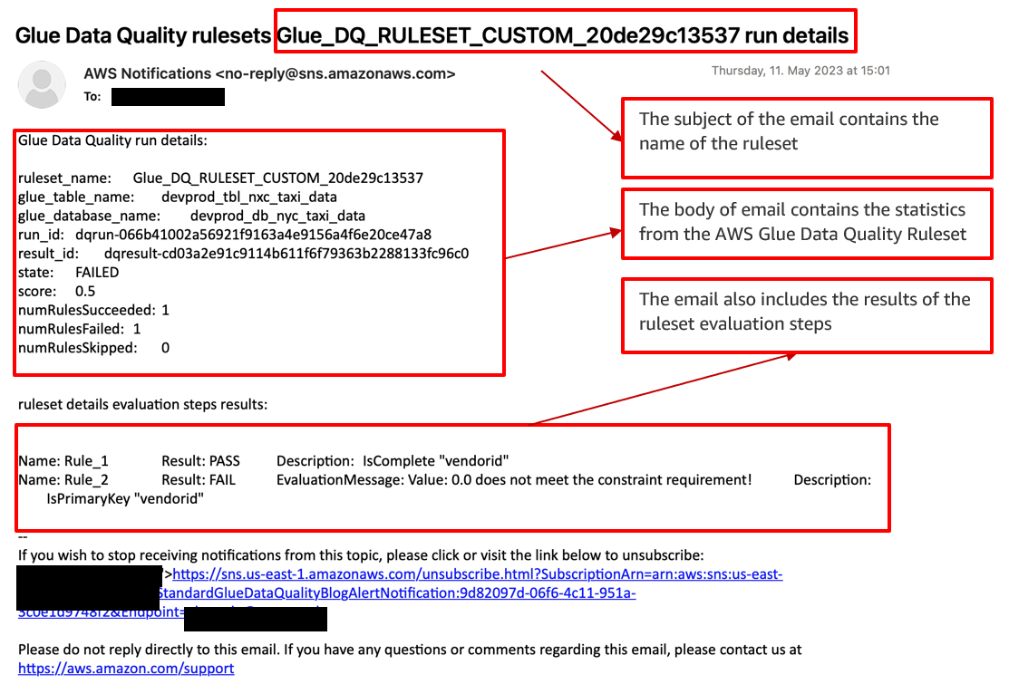
You have the flexibility to choose between two run modes for the Step Functions workflow:
- The first option is on-demand mode, where you manually trigger the Step Functions workflow whenever you want to initiate the AWS Glue Data Quality evaluation.
- Alternatively, you can schedule the entire Step Functions workflow using EventBridge. With EventBridge, you can define a schedule or specific triggers to automatically initiate the workflow at predetermined intervals or in response to specific events. This automated approach reduces the need for manual intervention and streamlines the data quality evaluation process. For more details, refer to Schedule a Serverless Workflow.
Clean up
To avoid incurring future charges and to clean up unused roles and policies, delete the resources you created:
- On the AWS CloudFormation console, choose Stacks in the navigation pane.
- Select your stack and delete it.
If you’re continuing to Part 5 in this series, you can skip this step.
Conclusion
In this post, we discussed three key steps that organizations can take to optimize data quality and reliability on AWS:
- Create a CloudFormation template to ensure consistency and reproducibility in deploying AWS resources.
- Integrate AWS Glue Data Quality ruleset evaluation and Lambda to automatically evaluate data quality and receive event-driven alerts and email notifications via Amazon SNS. This significantly enhances the accuracy and reliability of your data.
- Use Step Functions to orchestrate AWS Glue Data Quality ruleset actions. You can create and evaluate custom and recommended rulesets, optimizing data quality and accuracy.
These steps form a comprehensive approach to data quality and reliability on AWS, helping organizations maintain high standards and achieve their goals.
To dive into the AWS Glue Data Quality APIs, refer to Data Quality APIs. To learn more about AWS Glue Data Quality, check out the AWS Glue Data Quality Developer Guide.
If you require any assistance in constructing this pipeline within the AWS Lake Formation environment or if you have any inquiries regarding this post, please inform us in the comments section or initiate a new thread on the Lake Formation forum.
About the authors
Avik Bhattacharjee is a Senior Partner Solution Architect at AWS. He works with customers to build IT strategy, making digital transformation through the cloud more accessible, focusing on big data and analytics and AI/ML.
Amit Kumar Panda is a Data Architect at AWS Professional Services who is passionate about helping customers build scalable data analytics solutions to enable making critical business decisions.
 Neel Patel is a software engineer working within GlueML. He has contributed to the AWS Glue Data Quality feature and hopes it will expand the repertoire for all AWS CloudFormation users along with displaying the power and usability of AWS Glue as a whole.
 Edward Cho is a Software Development Engineer at AWS Glue. He has contributed to the AWS Glue Data Quality feature as well as the underlying open-source project Deequ.
Data is the lifeblood of modern businesses. In today’s data-driven world, companies rely on data to make informed decisions, gain a competitive edge, and provide exceptional customer experiences. However, not all data is created equal. Poor-quality data can lead to incorrect insights, bad decisions, and lost opportunities.
AWS Glue Data Quality measures and monitors the quality of your dataset. It supports both data quality at rest and data quality in AWS Glue extract, transform, and load (ETL) pipelines. Data quality at rest focuses on validating the data stored in data lakes, databases, or data warehouses. It ensures that the data meets specific quality standards before it is consumed. Data quality in ETL pipelines, on the other hand, ensures the quality of data as it moves through the ETL process. It helps identify data quality issues during the ETL pipeline, allowing for early detection and correction of problems and prevents the failure of the data pipeline because of data quality issues.
This is Part 3 of a five-post series on AWS Glue Data Quality. In this post, we demonstrate the advanced data quality checks that you can typically perform when bringing data from a database to an Amazon Simple Storage Service (Amazon S3) data lake. Check out the other posts in this series:
- Part 1: Getting started with AWS Glue Data Quality from the AWS Glue Data Catalog
- Part 2: Getting started with AWS Glue Data Quality for ETL Pipelines
- Part 3: Set up data quality rules across multiple datasets using AWS Glue Data Quality
- Part 4: Set up alerts and orchestrate data quality rules with AWS Glue Data Quality
- Part 5: Visualize data quality score and metrics generated by AWS Glue Data Quality
Use case overview
Let’s consider an example use case where we have a database named classicmodels that contains retail data for a car dealership. This example database includes sample data for various entities, such as Customers, Products, ProductLines, Orders, OrderDetails, Payments, Employees, and Offices. You can find more details about this example database in MySQL Sample Database.
In this scenario, we assume the role of a data engineer who is responsible for building a data pipeline. The primary objective is to extract data from a relational database, specifically an Amazon RDS for MySQL database, and store it in Amazon S3, which serves as a data lake. After the data is loaded into the data lake, the data engineer is also responsible for performing data quality checks to ensure that the data in the data lake maintains its quality. To achieve this, the data engineer uses the newly launched AWS Glue Data Quality evaluation feature.
The following diagram illustrates the entity relationship model that describes the relationships between different tables. In this post, we use the employees, customers, and products table.

Solution overview
This solution focuses on transferring data from an RDS for MySQL database to Amazon S3 and performing data quality checks using the AWS Glue ETL pipeline and AWS Glue Data Catalog. The workflow involves the following steps:
- Data is extracted from the RDS for MySQL database using AWS Glue ETL.
- The extracted data is stored in Amazon S3, which serves as the data lake.
- The Data Catalog and AWS Glue ETL pipeline are utilized to validate the successful completion of data ingestion by performing data quality checks on the data stored in Amazon S3.
The following diagram illustrates the solution architecture.

To implement the solution, we complete the following steps:
- Set up resources with AWS CloudFormation.
- Establish a connection to the RDS for MySQL instance from AWS Cloud9.
- Run an AWS Glue crawler on the RDS for MySQL database.
- Validate the Data Catalog.
- Run an AWS Glue ETL job to bring data from Amazon RDS for MySQL to Amazon S3.
- Evaluate the advanced data quality rules in the ETL job.
- Evaluate the advanced data quality rules in the Data Catalog.
Set up resources with AWS CloudFormation
This post includes a CloudFormation template for a quick setup. You can review and customize it to suit your needs. The template generates the following resources:
- An RDS for MySQL database instance (source)
- An S3 bucket for the data lake (destination)
- An AWS Glue ETL job to bring data from source to destination
- An AWS Glue crawler to crawl the RDS for MySQL databases and create a centralized Data Catalog
- AWS Identity and Access Management (IAM) users and policies
- An AWS Cloud9 environment to connect to the RDS DB instance and create a sample dataset
- An Amazon VPC, public subnet, two private subnets, internet gateway, NAT gateway, and route tables
To launch the CloudFormation stack, complete the following steps:
- Sign in to the AWS CloudFormation console.
- Choose Launch Stack:

- Choose Next.
- For DatabaseUserPassword, enter your preferred password.
- Choose Next.
- Scroll to the end and choose Next.
- Select I acknowledge that AWS CloudFormation might create IAM resources with custom names and choose Submit.
This stack can take around 10 minutes to complete, after which you can view the deployed stack on the AWS CloudFormation console.

Establish a connection to the RDS for MySQL instance from AWS Cloud9
To connect to the RDS for MySQL instance, complete the following steps:
- On the AWS Cloud9 console, choose Open under Cloud9 IDE for your environment.

- Run the following command to the AWS Cloud9 terminal. Provide your values for the MySQL endpoint (located on the CloudFormation stack’s Outputs tab), database user name, and database user password:
- Download the SQL file.
- On the File menu, choose Upload from Local Files and upload the file to AWS Cloud9.
- Run the following SQL commands within the downloaded file:
- Retrieve a list of tables using the following SQL statement and make sure that eight tables are loaded successfully:

Run an AWS Glue crawler on the RDS for MySQL database
To run your crawler, complete the following steps:
- On the AWS Glue console, choose Crawlers under Data Catalog in the navigation pane.
- Locate and run the crawler
dq-rds-crawler.
The crawler will take a few minutes to crawl all the tables from the classicmodels database.

Validate the AWS Glue Data Catalog
To validate the Data Catalog when the crawler is complete, complete the following steps:
- On the AWS Glue console, choose Databases under Data Catalog in the navigation pane.
- Choose the
mysql\_private\_classicmodelsdatabase.
You will able to see all the RDS tables available under mysql\_private\_classicmodels.

Run an AWS Glue ETL job to bring data from Amazon RDS for MySQL to Amazon S3
To run your ETL job, complete the following steps:
- On the AWS Glue console, choose Visual ETL under ETL jobs in the navigation pane.
- Select
dq-rds-to-s3from the job list and choose Run job.

When the job is complete, you will able to see three new tables under mysql\_s3\_db. It may take a few minutes to complete.

Now let’s dive into evaluating the data quality rules.
Evaluate the advanced data quality rules in the ETL job
In this section, we evaluate the results of different data quality rules.
ReferentialIntegrity
Let’s start with referential integrity. The ReferentialIntegrity data quality ruleset is currently supported in ETL jobs. This feature ensures that the relationships between tables in a database are maintained. It checks if the foreign key relationships between tables are valid and consistent, helping to identify any referential integrity violations.
- On the AWS Glue console, choose Visual ETL under ETL jobs in the navigation pane.
- In AWS Glue Studio, select Visual with a blank canvas.
- Provide a name for your job; for example, RDS
ReferentialIntegrity. - Choose the plus sign in the AWS Glue Studio canvas and on the Data tab, choose AWS Glue Data Catalog.
- For Name, enter a name for your data source; for example, employees.
- For Database, choose
mysql\_private\_classicmodels. - For Table, choose
mysql\_classicmodels\_employees.
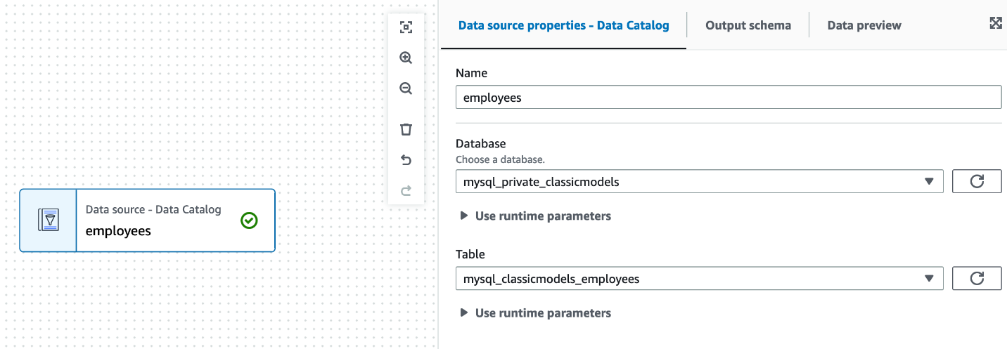
- Choose the plus sign in the AWS Glue Studio canvas and on the Data tab, choose AWS Glue Data Catalog.
- For Name, enter a name for your data source; for example,
customers. - For Database, choose
mysql\_private\_classicmodels. - For Table, choose
mysql\_classicmodels\_employees. - Choose the plus sign in the AWS Glue Studio canvas and on the Transform tab, choose Evaluate Data Quality.
- For Node parents, choose
employeesandcustomers. - For Aliases for referenced data source, select Primary source for employees and for customers, enter the alias customers.
All other datasets are used as references to ensure that the primary dataset has good-quality data.

- Search for
ReferentialIntegrityunder Rule types and choose the plus sign to add an exampleReferentialIntegrityrule.

- Replace the rule with the following code and keep the remaining options as default:
- Under Data quality action, select Publish results to Amazon CloudWatch and select Fail job without loading target data.
- On the Job details tab, choose
GlueServiceRole-for-gluedq-blogfor IAM role and keep the remaining options as default. - Choose Run and wait for the job to complete.
It will take a few minutes to complete.
- When the job is complete, navigate to the Data quality tab and locate the Data quality results section.
You can confirm if the job completed successfully and which data quality rules it passed. In this example, it indicates that 60–70% of EmployeeNumber from the employees table are present in the customers table.

You can identify which records failed the referential integrity using AWS Glue Studio. To learn more, refer to Getting started with AWS Glue Data Quality for ETL Pipelines.
Similarly, if you are checking if all the EmployeeNumber from the employees table are present in the customers table, you can pass the following rule:
DatasetMatch
DatasetMatch compares two datasets to identify differences and similarities. You can use it to detect changes between datasets or to find duplicates, missing values, or inconsistencies across datasets.
- On the AWS Glue console, choose Visual ETL under ETL jobs in the navigation pane.
- In AWS Glue Studio, select Visual with a blank canvas.
- Provide a name for your job; for example,
RDS DatasetMatch. - Choose the plus sign in the AWS Glue Studio canvas and on the Data tab, choose AWS Glue Data Catalog.
- For Name, enter a name for your data source; for example,
rds\_employees\_primary. - For Database, choose
mysql\_private\_classicmodels. - For Table, choose
mysql\_classicmodels\_employees. - Choose the plus sign in the AWS Glue Studio canvas and on the Data tab, choose AWS Glue Data Catalog.
- For Name, enter a name for your data source; for example,
s3\_employees\_reference. - For Database, choose
mysql\_s3\_db. - For Table, choose
s3\_employees. - Choose the plus sign in the AWS Glue Studio canvas and on the Transform tab, choose Evaluate Data Quality.
- For Node parents, choose
employeesandcustomers. - For Aliases for referenced data source, select Primary source for
rds\_employees\_primaryand fors3\_employees\_reference, enter the aliasreference.

- Replace the default example rules with the following code and keep the remaining options as default:
- On the Job details tab, choose
GlueServiceRole-for-gluedq-blogfor IAM role and keep the remaining options as default. - Choose Run and wait for the job to complete.
- When the job is complete, navigate to the Data quality tab and locate the Data quality results section.
In this example, it indicates both datasets are identical.

AggregateMatch
AggregateMatch verifies the accuracy of aggregated data. It compares the aggregated values in a dataset against the expected results to identify any discrepancies, such as incorrect sums, averages, counts, or other aggregate calculations. This is a performant option to evaluate if two datasets match at an aggregate level. For this rule, we clone the previous job we created for DatasetMatch.
- On the AWS Glue console, choose Visual ETL under ETL jobs in the navigation pane.
- Select
RDS DatasetMatchand on the Actions menu, choose Clone job.

- Change the job name to
DQ AggregateMatch. - Change the dataset
rds\_employees\_primaryto rds\_products\_primary and the table tomysql\_classicmodels\_products. - Change the dataset
s3\_orders\_referencetos3\_products\_referenceand the table tos3\_products. - Choose Evaluate Data Quality, and under Node parents, choose
rds\_products\_primaryands3\_products\_reference. - Replace the rules with the following code:

- Choose Run and wait for the job to complete.
- When the job is complete, navigate to the Data quality tab and locate the Data quality results section.
The results indicate that the avg(msrp) on both datasets is the same.

RowCountMatch
RowCountMatch checks the number of rows in a dataset and compares it to an expected count. It helps identify missing or extra rows in a dataset, ensuring data completeness. For this rule, we edit the job we created earlier for AggregateMatch.
- On the AWS Glue console, choose Visual ETL under ETL jobs in the navigation pane.
- Select RDS
AggregateMatchand on the Actions menu, choose Edit job.

- Choose Evaluate Data Quality and choose the plus sign next to
RowCountMatch.

- Keep the default data quality rules and choose Save:
RowCountMatch "reference" = 1.0
- Choose Run and wait for the job to complete.
- When the job is complete, navigate to the Data quality tab and locate the Data quality results section.
It shows that the DQ RowCountMatch rule failed, indicating a mismatch between the row count of the source RDS table and the target S3 table. Further investigation reveals that the ETL job ran four times for the Products table, and the row counts didn’t match.
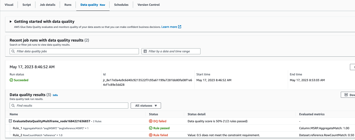
SchemaMatch
SchemaMatch validates the schema of two datasets matches. It checks if the actual data types match the expected data types and flags any inconsistencies, such as a numeric column containing non-numeric values. For this rule, we edit the job we used for AggregateMatch.
- On the AWS Glue console, choose Visual ETL under ETL jobs in the navigation pane.
- Select
RDS AggregateMatchand on the Actions menu, choose Edit job.

- Choose Evaluate Data Quality and choose the plus sign next to
RowCountMatch. - Update the default rules with the following code and save the job:

- Choose Run and wait for the job to complete.
- When the job is complete, navigate to the Data quality tab and locate the Data quality results section.
It should show a successful completion with a Rule passed status, indicating that the schemas of both datasets are identical.

Evaluate the advanced data quality rules in the Data Catalog
The AWS Glue Data Catalog also supports advanced data quality rules. For this post, we show one example of an aggregate match between Amazon S3 and Amazon RDS.
- On the AWS Glue console, choose Databases in the navigation pane.
- Choose the
mysql\_private\_classicmodelsdatabase to view the three tables created under it. - Choose the
mysql\_classicmodels\_productstable. - On the Data quality tab, choose Create data quality rules.

- Search for
AggregateMatchand choose the plus sign to view the default example rule. - Add the following rules:
reference is the alias of the secondary dataset defined in the AWS Glue ETL job. For the Data Catalog, you can use <database\_name>.<table\_name>.<column\_name> to reference secondary datasets.
- Choose Save ruleset and provide the name
production\_catalog\_dq\_check. - Choose
GlueServiceRole-for-gluedq-blogfor IAM role and keep the remaining options as default. - Choose Run and wait for the data quality check to complete.
When the job is complete, you can confirm that both data quality checks passed.

With these advanced data quality features of AWS Glue Data Quality, you can enhance the reliability, accuracy, and consistency of your data, leading to better insights and decision-making.
Clean up
To clean up your resources, complete the following steps:
- Delete the AWS Glue job.
- Delete the CloudFormation stack.
Conclusion
Data quality refers to the accuracy, completeness, consistency, timeliness, and validity of the information being collected, processed, and analyzed. High-quality data is essential for businesses to make informed decisions, gain valuable insights, and maintain their competitive advantage. As data complexity increases, advanced rules are critical to handle complex data quality challenges. The rules we demonstrated in this post can help you manage the quality of data that lives in disparate data sources, providing you the capabilities to reconcile them. Try them out and provide your feedback on what other use cases you need to solve!
About the authors
 Navnit Shukla is AWS Specialist Solutions Architect in Analytics. He is passionate about helping customers uncover insights from their data. He builds solutions to help organizations make data-driven decisions.
 Rahul Sharma is a Software Development Engineer at AWS Glue. He focuses on building distributed systems to support features in AWS Glue. He has a passion for helping customers build data management solutions on the AWS Cloud.
Edward Cho is a Software Development Engineer at AWS Glue. He has contributed to the AWS Glue Data Quality feature as well as the underlying open-source project Deequ.
 Shriya Vanvari is a Software Developer Engineer in AWS Glue. She is passionate about learning how to build efficient and scalable systems to provide better experience for customers. Outside of work, she enjoys reading and chasing sunsets.
AWS Glue is a serverless data integration service that makes it simple to discover, prepare, and combine data for analytics, machine learning (ML), and application development. You can use AWS Glue to create, run, and monitor data integration and ETL (extract, transform, and load) pipelines and catalog your assets across multiple data stores.
Hundreds of thousands of customers use data lakes for analytics and ML to make data-driven business decisions. Data consumers lose trust in data if it isn’t accurate and recent, making data quality essential for undertaking optimal and correct decisions.
Evaluation of the accuracy and freshness of data is a common task for engineers. Currently, various tools are available to evaluate data quality. However, these tools often require manual processes of data discovery and expertise in data engineering and coding.
AWS Glue Data Quality is a new feature of AWS Glue that measures and monitors the data quality of Amazon Simple Storage Service (Amazon S3)-based data lakes, data warehouses, and other data repositories. AWS Glue Data Quality can be accessed in the AWS Glue Data Catalog and in AWS Glue ETL jobs.
This is Part 1 of a five-part series of posts to explain how AWS Glue Data Quality works. Check out the next posts in the series:
- Part 1: Getting started with AWS Glue Data Quality from the AWS Glue Data Catalog
- Part 2: Getting started with AWS Glue Data Quality for ETL Pipelines
- Part 3: Set up data quality rules across multiple datasets using AWS Glue Data Quality
- Part 4: Set up alerts and orchestrate data quality rules with AWS Glue Data Quality
- Part 5: Visualize data quality score and metrics generated by AWS Glue Data Quality
In this post, we explore using the AWS Glue Data Quality feature by generating data quality recommendations and running data quality evaluations on your table in the Data Catalog. Then we demonstrate how to analyze your AWS Glue Data Quality run results through Amazon Athena.
Solution overview
We guide you through the following steps:
- Provision resources with AWS CloudFormation.
- Explore the generated recommendation rulesets and define rulesets to evaluate your table in the Data Catalog.
- Review the AWS Glue Data Quality recommendations.
- Analyze your AWS Glue Data Quality evaluation results with Athena.
- Operationalize the solution by setting up alerts and notifications using integration with Amazon EventBridge and Amazon Simple Notification Service (Amazon SNS).
For this post, we use the NYC Taxi dataset yellow\_tripdata\_2022-01.parquet.
Set up resources with AWS CloudFormation
The provided CloudFormation template creates the following resources for you:
- The AWS Identity and Access Management (IAM) role required to run AWS Glue Data Quality evaluations
- An S3 bucket to store the NYC Taxi dataset
- An S3 bucket to store and analyze the results of AWS Glue Data Quality evaluations
- An AWS Glue database and table created from the NYC Taxi dataset
Launch your CloudFormation stack
To create your resources for this use case, complete the following steps:
- Launch your CloudFormation stack in
us-east-1:
- Under Parameters:
- For Stack name, proceed with the default value
myDQStack. - For DataQualityDatabase, proceed with the default value
data\_quality\_catalog. - For DataQualityS3BucketName, provide a bucket name of your choice.
- For DataQualityTable, proceed with the default value
data\_quality\_tripdata\_table

- For Stack name, proceed with the default value
- Select I acknowledge that AWS CloudFormation might create IAM resources with custom names.
- Choose Create stack.
After the stack is successfully created, you can see all the resources created on the Resources tab.

- Navigate to the S3 bucket created by the stack and upload the yellow\_tripdata\_2022-01.parquet file.
Explore recommendation rulesets and define rulesets to evaluate your table
In this section, we generate data quality rule recommendations from AWS Glue Data Quality. We use these recommendations to run a data quality task against our dataset to obtain an analysis of our data.
Complete the following steps:
- On the AWS Glue console, under Data Catalog in the navigation pane, choose Tables.
- Choose the
data\_quality\_tripdata\_tabletable created via the CloudFormation stack. - Choose the Data quality tab.
In this section, you will find a video to get you started with AWS Glue Data Quality. It also lists features, pricing, and documentation.
- Choose Create data quality rules.
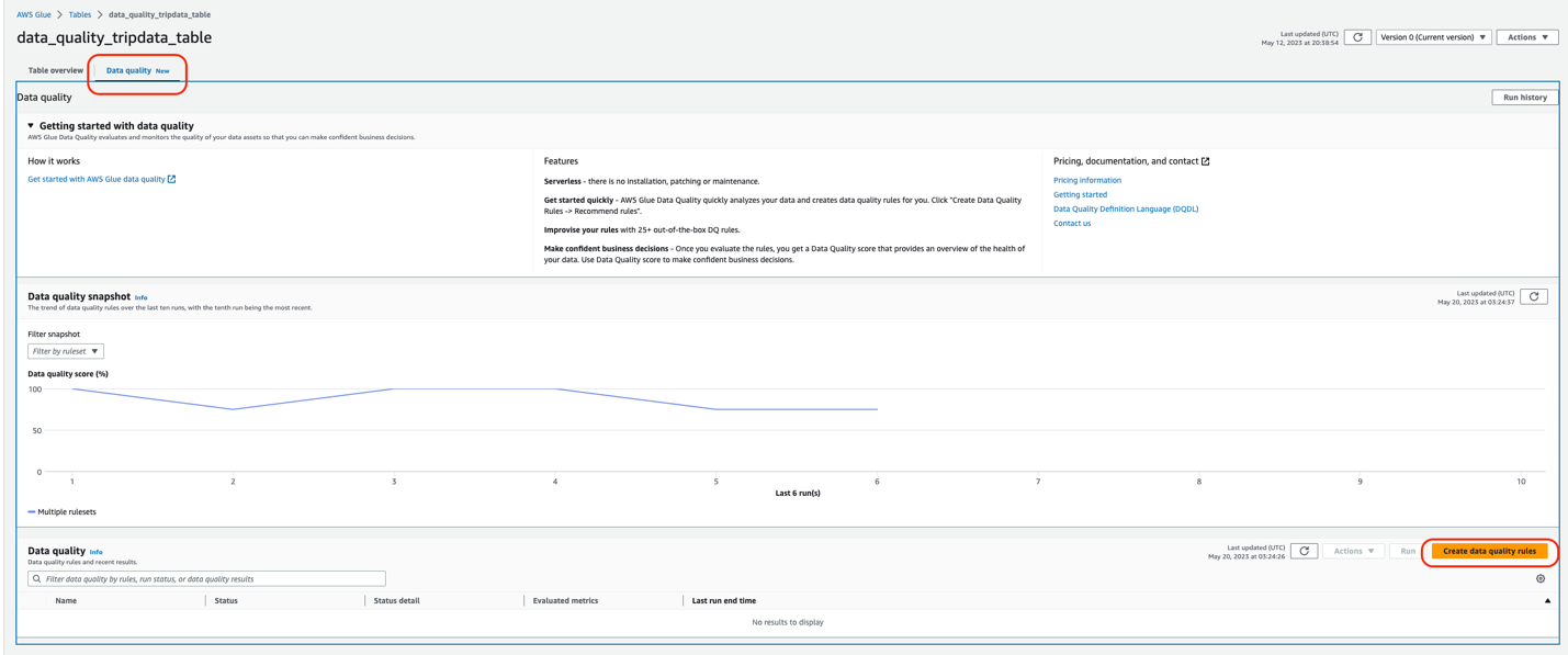
This is the ruleset console. You will find a Request data quality rule recommendations banner at the top. AWS Glue will scan your data and automatically generate rule recommendations.
- Choose Recommend rules.

- For IAM role, choose the IAM role created as part of the Cloud Formation template (
GlueDataQualityBlogRole). - Optionally, you can filter your data before reading on column values. This feature is available for Amazon S3-based data sources.
- For Requested number of workers, allocate the number of workers to run the recommendation task. For this post, we use the default value of 5.
- For Task timeout, set the runtime for this task. For this post, we use the default of 120 minutes.
- Choose Recommend rules.

The recommendation task will start instantly, and you will observe the status on the top changes to Starting.
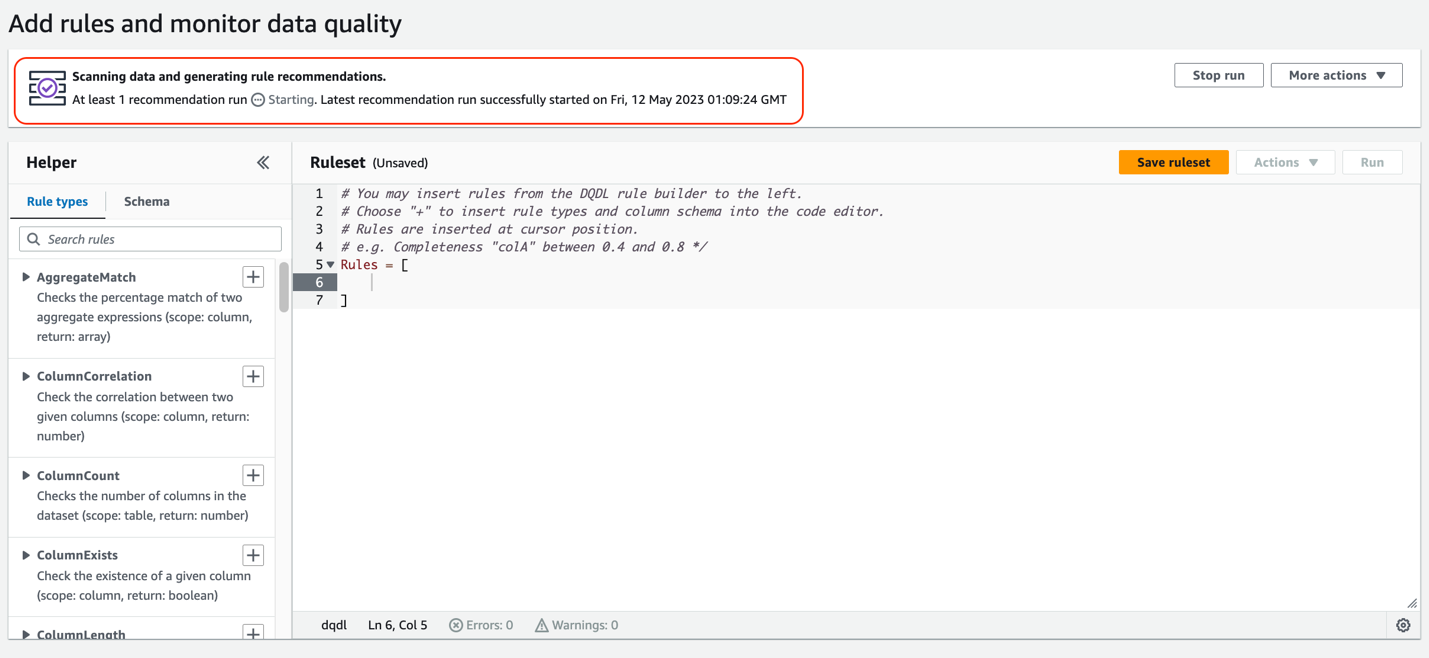
Next, we add some of these recommended rules into our ruleset.
- When you see the recommendation run as Completed, choose Insert rule recommendations to select the rules that are recommended for you.
Make sure to place the cursor inside the brackets Rules = [ ].

- Select the following rules:
ColumnValues “VendorID” <=6Completeness “passenger\_count”>=0.97
- Choose Add selected rules.
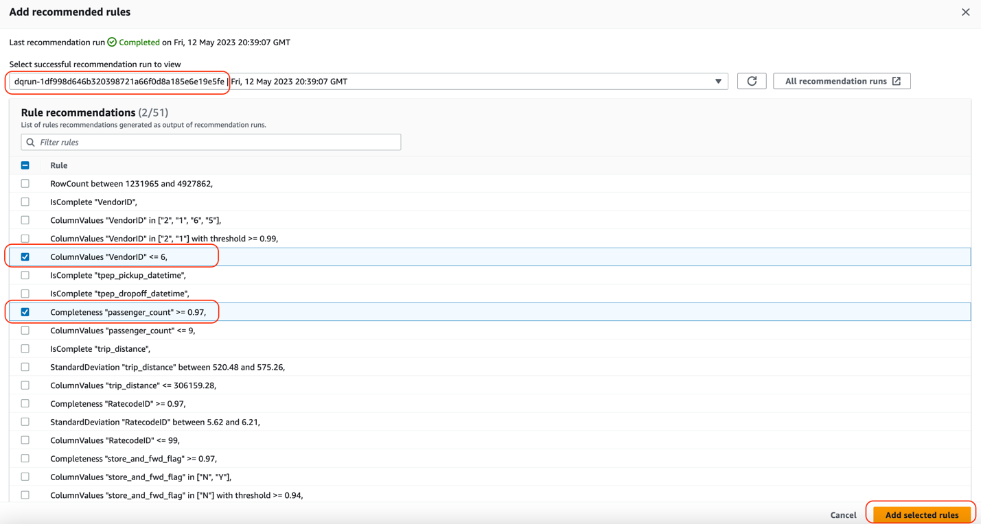
You can see that these rules were automatically added to the ruleset.
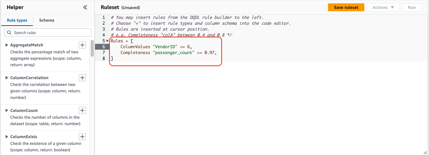
Understanding AWS Glue Data Quality recommendations
AWS Glue Data Quality recommendations are suggestions generated by the AWS Glue Data Quality service and are based on the shape of your data. These recommendations automatically take into account aspects like row counts, mean, standard deviation, and so on, and generate a set of rules for you to use as a starting point.
The dataset used here was the NYC Taxi dataset. Based on this, the columns in this dataset, and the values of those columns, AWS Glue Data Quality recommends a set of rules. In total, the recommendation service automatically took into consideration all the columns of the dataset, and recommended 55 rules.
Some of these rules are:
- ColumnValues “VendorID” <=6 – The
ColumnValuesrule type checks the percentage of complete (non-null) values in a column against a given expression. This rule resolves to true if the rule type response is less than or equal to value 6. - Completeness “passenger\_count”>=0.97 – The
Completenessrule type checks the percentage of complete (non-null) values in a column against a given expression. In this case, the rule checks if more than 97% of the values in a column are complete.

In addition to adding auto-generated recommendation rules, we manually add some rules to the ruleset. AWS Glue Data Quality provides some out-of-the-box rule types to choose from. For this post, we manually add the IsComplete rule for VendorID.
- In the left pane, on the Rule types tab, search
IsCompleterule type and choose the plus sign next toIsCompleteto add this rule. - For the value within the quotation marks, enter
VendorID.
Conversely, you could navigate to the Schema tab and add IsComplete to VendorID.
- Choose Save ruleset.

Next, we add a CustomSQL rule by selecting the rule type CustomSql, that validates that there are no fares charged for a trip if there are no passengers. This is to identify if there are any fraudulent transactions for fare\_amount > 0 where passenger\_count = 0. The rule is:
There are two ways to provide the table name:
- Either you can use the keyword “primary” for the table under consideration
- You can use the full path such as
database\_name.table\_name
- On the Rule types tab, choose the plus sign next to CustomSQL and enter the SQL statement.

The final ruleset looks like the following screenshot.

- Choose Save ruleset.
- For Ruleset name, enter a name.
- Choose Save ruleset.

- On the ruleset page, choose Run.

- For IAM role¸ choose
GlueDataQualityBlogRole. - Select Publish run metrics to Amazon CloudWatch.
- For Data quality result location, enter the S3 bucket location for the data quality results which is already created for you as part of Cloud Formation template (for this post,
data-quality-tripdata-results). - For Run frequency, choose On demand.

- Expand Additional configurations.
- For Requested number of workers, enter
5. - Leave the remaining fields as is and choose Run.
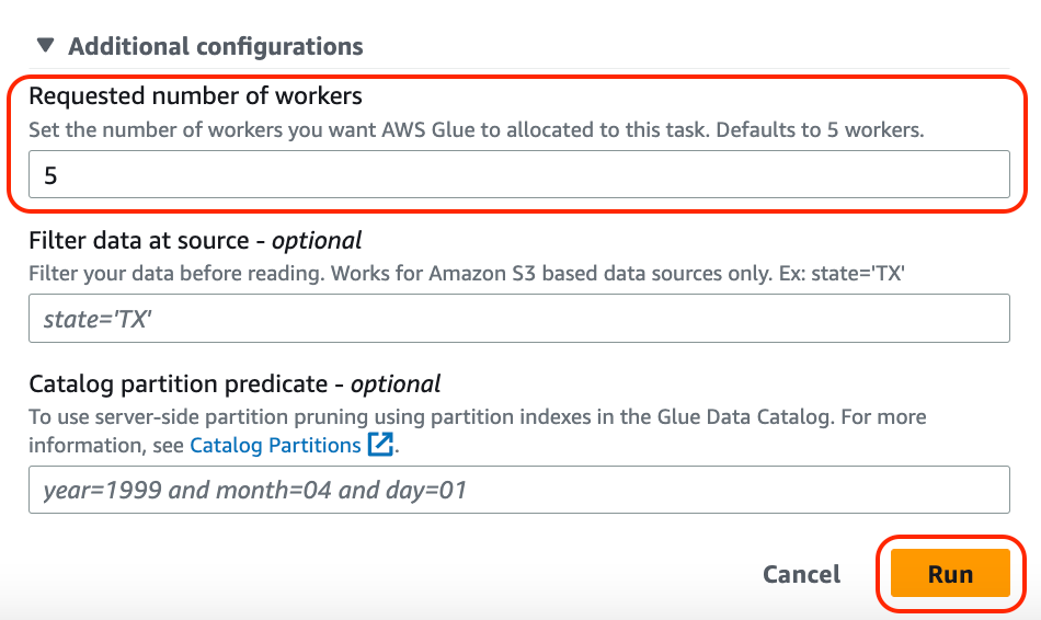
The status changes to Starting.

- When it’s complete, choose the ruleset and choose Run history.
- Choose the run ID to find more about the run details.

Under Data quality result, you will also observe the result shows as DQ passed or DQ failed.

In the Evaluation run details section, you will find all the details about the data quality task run and rules that passed or failed. You can either view these results by navigating to the S3 bucket or downloading the results. Observe that the data quality task failed because one of the rules failed.
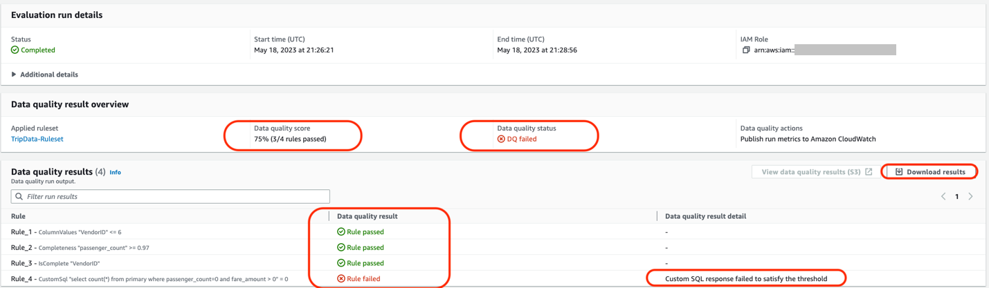
For the first section, AWS Glue Data Quality suggested 51 rules, based on the column values and the data within our NYC Taxi dataset. We selected a few rules out of the 51 rules into a ruleset and ran an AWS Glue Data Quality evaluation task using our ruleset against our dataset. In our results, we see the status of each rule within the run details of the data quality task.
You can also utilize the AWS Glue Data Quality APIs to carry out these steps.
Analyze your AWS Glue Data Quality evaluation results with Athena
If you have multiple AWS Glue Data Quality evaluation results against a dataset, you might want to track the trends of the dataset’s quality over a period of time. To achieve this, we can export our AWS Glue Data Quality evaluation results to Amazon S3, and use Athena to run analytical queries against the exported results. You could further use the results in Amazon QuickSight to build dashboards to have a graphical representation of your data quality trends
In Part 3 of this series, we show the steps needed to start tracking data on your dataset’s quality.
For our data quality runs that we set up in the previous sections, we set the Data quality results location parameter to the bucket location specified by the CloudFormation stack. After each successful run, you should see a Parquet format file that contains a single JSONL file being exported to your selected S3 location, corresponding to that particular run.
Complete the following steps to analyze the data:
- Navigate to Amazon Athena and on the console, navigate to Query Editor.
- Run the following CREATE TABLE statement (replace the <my\_table\_name> with a relevant value of your choice and <GlueDataQualityResultsS3Bucket\_from\_cfn> with the S3 bucket name to store data-quality results; the bucket name will have trailing keyword
results, for example <given-name-results>. For this post, it isdata-quality-tripdata-results.
After you create the table, you should be able to run queries to analyze your data quality results.
For example, consider the following query that shows the passed AWS Glue Data Quality evaluations against the table data\_quality\_tripdata\_table within a certain time window. You can select the datetime values from the data quality results table (that you created above) <my\_table\_name> from the columns evaluationcompletedon to specify values for parse\_datetime() within a certain duration in the following query:
The output of the preceding query shows us details about all the runs with “outcome” = ‘Passed’ that ran against the NYC Taxi dataset table (“tablename” = ‘data\_quality\_tripdata\_table’). The output also provides details about the rules passed and evaluated metrics.
As you can see, we are able to get detailed information about our AWS Glue Data Quality evaluations via the results uploaded to Amazon S3 and perform more detailed analysis.
Set up alerts and notifications using EventBridge and Amazon SNS
Alerts and notifications are important for data quality to enable timely and effective responses to data quality issues that arise in the dataset. By setting up alerts and notifications, you can proactively monitor the data quality and be alerted as soon as any data quality issues are detected. This reduces the risk of making decisions based on incorrect information.
AWS Glue Data Quality also offers integration with EventBridge for alerting and notification by triggering an AWS Lambda function that sends a customized SNS notification when the AWS Glue Data Quality ruleset evaluation is complete. Now you can receive event-driven alerts and email notifications via Amazon SNS. This integration significantly enhances the accuracy and reliability of data.
Clean up
To clean up your resources, complete the following steps:
- On the Athena console, delete the table created for data quality analysis.
- On the CloudWatch console, delete the alarms created.
- If you deployed the sample CloudFormation stack, delete the stack via the AWS CloudFormation console. You will need to empty the S3 bucket before you delete the bucket.
- If you enabled your AWS Glue Data Quality runs to output to Amazon S3, empty those buckets as well.
Conclusion
In this post, we talked about the ease and speed of incorporating data quality rules using AWS Glue Data Quality into your Data Catalog tables. We also talked about how to run recommendations and evaluate data quality against your tables. We then discussed analyzing the data quality results via Athena, and discussed integrations with EventBridge and Amazon SNS for alerts and notifications to get notified for data quality issues.
To dive into the AWS Glue Data Quality APIs, refer to Data Quality API documentation. To learn more about AWS Glue Data Quality, check out AWS Glue Data Quality.
About the authors
 Stuti Deshpande is an Analytics Specialist Solutions Architect at AWS. She works with customers around the globe, providing them strategic and architectural guidance on implementing analytics solutions using AWS. She has extensive experience in Big Data, ETL, and Analytics. In her free time, Stuti likes to travel, learn new dance forms, and enjoy quality time with family and friends.
 Aniket Jiddigoudar is a Big Data Architect on the AWS Glue team. He works with customers to help improve their big data workloads. In his spare time, he enjoys trying out new food, playing video games, and kickboxing.
 Joseph Barlan is a Frontend Engineer at AWS Glue. He has over 5 years of experience helping teams build reusable UI components and is passionate about frontend design systems. In his spare time, he enjoys pencil drawing and binge watching tv shows.
 Jesus Max Hernandez is a Software Development Engineer at AWS Glue. He joined the team in August after graduating from The University of Texas at El Paso. Outside of work, you can find him practicing guitar or playing softball in Central Park.
 Divya Gaitonde
is a UX designer at AWS Glue. She has over 8 years of experience driving impact through data-driven products and seamless experiences. Outside of work, you can find her catching up on reading or people watching at a museum.
In the first post of the series, we described some core concepts of Apache Kafka cluster sizing, the best practices for optimizing the performance, and the cost of your Kafka workload.
This post explains how the underlying infrastructure affects Kafka performance when you use Amazon Managed Streaming for Apache Kafka (Amazon MSK) tiered storage. We delve deep into the core components of Amazon MSK tiered storage and address questions such as: How does read and write work in a tiered storage-enabled cluster?
In the subsequent post, we’ll discuss the latency impact, recommended metrics to monitor, and conclude with guidance on key considerations in a production tiered storage-enabled cluster.
How Amazon MSK tiered storage works
To understand the internal architecture of Amazon MSK tiered storage, let’s first discuss some fundamentals of Kafka topics, partitions, and how read and write works.
A logical stream of data in Kafka is referred to as a topic. A topic is broken down into partitions, which are physical entities used to distribute load across multiple server instances (brokers) that serve reads and writes.
A partition––also designated as topic-partition as it’s relative to a given topic––can be replicated, which means there are several copies of the data in the group of brokers forming a cluster. Each copy is called a replica or a log. One of these replicas, called the leader, serves as the reference. It’s where the ingress traffic is accepted for the topic-partition.
A log is an append-only sequence of log segments. Log segments contain Kafka data records, which are added to the end of the log or the active segment.
Log segments are stored as regular files. On the file system, Kafka identifies the file of a log segment by putting the offset of the first data record it contains in its file name. The offset of a record is simply a monotonic index assigned to a record by Kafka when it’s appended to the log. The segment files of a log are stored in a directory dedicated to the associated topic-partition.
When Kafka reads data from an arbitrary offset, it first looks up the segment that contains that offset from the segment file name, then the specific record location inside that file using an offset index. Offset indexes are materialized on a dedicated file stored with segment files in the topic-partition directory. There is also timeindex to seek by timestamp.
For every partition, Kafka also stores a journal of leadership changes in a file called leader-epoch-checkpoint. This file contains mapping of leader epoch to startOffset of the epoch. Whenever a new leader is elected for a partition by the Kafka controller, this data is updated and propagated to all brokers. A leader epoch is a 32-bit, monotonically increasing number representing continuous period of leadership of a single partition. It’s marked on all the Kafka records. The following code is the local storage layout of topic cars and partition 0 containing two segments (0, 35):
Kafka manages the lifecycle of these segment files. It creates a new one when a new segment needs to be created, for instance, if the current segment reaches its configured max size. It deletes one when the target retention period of the data it contains is reached, or the total maximal size of the log is reached. Data is deleted from the tail of the logs and corresponds to the oldest data of the append-only log of the topic-partition.

KIP-405 or tiered storage in Apache Kafka
The ability to tier data, in other words, transfer data (log, index, timeindex, and leader-epoch-checkpoint) from a local file system to another storage system based on time and size-based retention policies, is a feature built in Apache Kafka as part of KIP-405.
The KIP-405 isn’t in official Kafka version yet. Amazon MSK internally implemented tiered storage functionality on top of official Kafka version 2.8.2. Amazon MSK exposes this functionality on AWS specific 2.8.2.tiered Kafka version. With this feature, you can separate retention settings for local and remote retention. Data in the local tier is retained until the data gets copied to the remote tier even after the local retention expires. Data in the remote tier is retained until the remote retention expires. KIP-405 proposes a pluggable architecture allowing you to plugin custom remote storage and metadata storage backends. The following diagram illustrates the broker three key components.
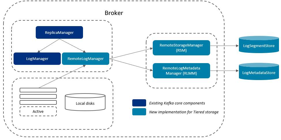
The components are as follows:
- RemoteLogManager (RLM) – A new component corresponding to LogManager for the local tier. It delegates copy, fetch, and delete of completed and non-active partition segments to a pluggable RemoteStorageManager implementation and maintains respective remote log segment metadata through pluggable RemoteLogMetadataManager implementation.
- RemoteStorageManager (RSM) – A pluggable interface that provides the lifecycle of remote log segments.
- RemoteLogMetadataManager (RLMM) – A pluggable interface that provides the lifecycle of metadata about remote log segments.
How data is moved to the remote tier for a tiered storage-enabled topic
In a tiered storage-enabled topic, each completed segment for a topic-partition triggers the leader of the partition to copy the data to the remote storage tier. The completed log segment is removed from the local disks when Amazon MSK finishes moving that log segment to the remote tier and after it meets the local retention policy. This frees up local storage space.
Let’s consider a hypothetical scenario: you have a topic with one partition. Prior to enabling tiered storage for this topic, there are three log segments. One of the segments is active and receiving data, and the other two segments are complete.
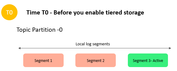
After you enable tiered storage for this topic with two days of local retention and five days of overall retention, Amazon MSK copies log segment 1 and 2 to tiered storage. Amazon MSK also retains the primary storage copy of segments 1 and 2. The active segment 3 isn’t eligible to copy over to tiered storage yet. In this timeline, none of the retention settings are applied yet for any of the messages in segment 1 and segment 2.
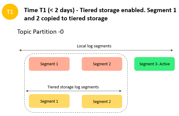
After 2 days, the primary retention settings take effect for the segment 1 and segment 2 that Amazon MSK copied to the tiered storage. Segments 1 and 2 now expire from the local storage. Active segment 3 is neither eligible for expiration nor eligible to copy over to tiered storage yet because it’s an active segment.
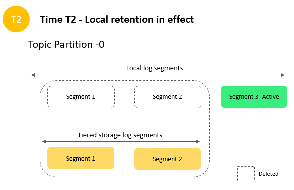
After 5 days, overall retention settings take effect, and Amazon MSK clears log segments 1 and 2 from tiered storage. Segment 3 is neither eligible for expiration nor eligible to copy over to tiered storage yet because it’s active.
That’s how the data lifecycle works on a tiered storage-enabled cluster.

Amazon MSK immediately starts moving data to tiered storage as soon as a segment is closed. The local disks are freed up when Amazon MSK finishes moving that log segment to remote tier and after it meets the local retention policy.
How read works in a tiered storage-enabled topic
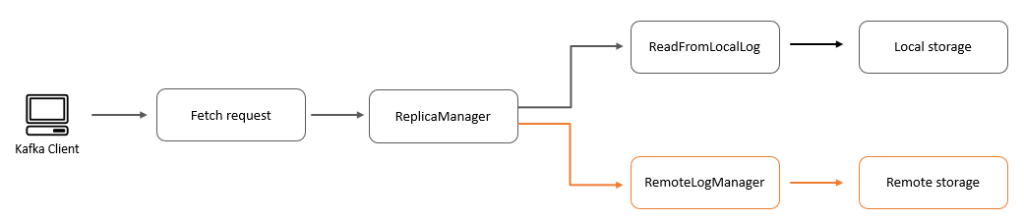
For any read request, ReplicaManager tries to process the request by sending it to ReadFromLocalLog. And if the process returns offset out of range exception, it delegates the read call to RemoteLogManager to read from tiered storage. On the read path, the RemoteStorageManager starts fetching the data in chunks from remote storage, which means that for the first few bytes, your consumer experiences higher latency, but as the system starts buffering the segment locally, your consumer experiences latency similar to reading from local storage. One of the advantages of this approach is that the data is served instantly from the local buffer if there are multiple consumers reading from the same segment.
If your consumer is configured to read from the closest replica, there might be a possibility that the consumer from a different consumer group reads the same remote segment using a different broker. In that case, they experience the same latency behavior we described previously.
Conclusion
In this post, we discussed the core components of the Amazon MSK tiered storage feature and explained how the data lifecycle works in a cluster enabled with tiered storage. Stay tuned for our upcoming post, in which we delve into the best practices for sizing and running a tiered storage-enabled cluster in production.
We would love to hear how you’re building your real-time data streaming applications today. If you’re just getting started with Amazon MSK tiered storage, we recommend getting hands-on with the guidelines available in the tiered storage documentation.
If you have any questions or feedback, please leave them in the comments section.
About the authors
 Nagarjuna Koduru is a Principal Engineer in AWS, currently working for AWS Managed Streaming For Kafka (MSK). He led the teams that built MSK Serverless and MSK Tiered storage products. He previously led the team in Amazon JustWalkOut (JWO) that is responsible for realtime tracking of shopper locations in the store. He played pivotal role in scaling the stateful stream processing infrastructure to support larger store formats and reducing the overall cost of the system. He has keen interest in stream processing, messaging and distributed storage infrastructure.
 Masudur Rahaman Sayem is a Streaming Data Architect at AWS. He works with AWS customers globally to design and build data streaming architectures to solve real-world business problems. He specializes in optimizing solutions that use streaming data services and NoSQL. Sayem is very passionate about distributed computing.
This is a guest blog post by Mira Daniels and Sean Whitfield from SumUp.
SumUp is a leading global financial technology company driven by the purpose of leveling the playing field for small businesses. Founded in 2012, SumUp is the financial partner for more than 4 million small merchants in over 35 markets worldwide, helping them start, run and grow their business. Through its Super App, SumUp provides merchants with a free business account and card, an online store, and an invoicing solution – as well as in-person and remote payments seamlessly integrated with SumUp’s card terminals and point-of-sale registers. For more information, please visit sumup.co.uk.
As most organizations, that have turned to Google Analytics (GA) as a digital analytics solution, mature they discover a more pressing need to integrate this data silo with the rest of their organization’s data to enable better analytics and resulting product development and fraud detection. Unless, of course, the rest of their data also resides in the Google Cloud. In this post we showcase how we used AWS Glue to move siloed digital analytics data, with inconsistent arrival times, to AWS S3 (our Data Lake) and our central data warehouse (DWH), Snowflake. AWS Glue gave us a cost-efficient option to migrate the data and we further optimized storage cost by pruning cold data. What was essential to the solution development was a good understanding of the nature of the data, the source of it (export from GA) as well as the form and scope of the data useful to the data consumers.
Business context
At SumUp we use GA and Firebase as our digital analytics solutions and AWS as our main Cloud Provider. In order to mature our data marts, it became clear that we needed to provide Analysts and other data consumers with all tracked digital analytics data in our DWH as they depend on it for analyses, reporting, campaign evaluation, product development and A/B testing. We further use the Digital Analytics data for our reverse ETL pipelines that ingest merchant behavior data back into the Ad tools. As the SumUp merchants user journey only starts onsite (with a Sign up or product purchase), but extends to offline card reader transactions or usage of our products from within our app and web dashboard, it is important to combine Digital Analytics data with other (backend) data sources in our Data Lake or DWH. The Data Science teams also use this data for churn prediction and CLTV modeling.
Given that the only source to access all raw data is by exporting it to BigQuery (first), data accessibility becomes challenging if BigQuery isn’t your DWH solution. What we needed was a data pipeline from BigQuery to our Data Lake and the DWH. The pipeline further needed to run based on the trigger of new data arriving in BigQuery and could not run on a simple schedule as data would not arrive at the same time consistently.
We experimented with some no-code tools that allowed for the direct export of Google Analytics data (not available for Firebase) from BigQuery directly to Snowflake, but due to our growing data volume, this wasn’t financially scalable. Other no-code tools, even if they can move data to S3, did not meet our technical requirements. The solutions we experimented with did not give us the flexibility to monitor and scale resources per pipeline run and optimize the pipeline ourselves.
We had a solid business case to build our own internal digital analytics pipeline to not only reduce spending on our existing outsourced Google Analytics pipeline (that moved from BigQuery to Snowflake directly), but also to make GA and Firebase data available in both the Data Lake and DWH.
Technical challenges
Data source specifics: The data in BigQuery is the export of GA 360 data and Firebase Analytics data. It consists of full-day and intraday tables. BigQuery uses a columnar storage format that can efficiently query semi-structured data, in the case of GA and Firebase data as arrays of structs.
Full-day: Daily tables that do not change retroactively for GA data, but for Firebase data
Intraday: Until the daily tables (full-day are created the intraday tables are populated with new and corrected records.
Update interval: intraday is refreshed and overwritten at least 3x a day. When the full-day table is created, the intraday table from that day is deleted.
Since we started exporting GA tracking data to BigQuery in 2015 the amount of data tracked and stored has grown 70x (logical bytes) and is >3TB in total. Our solution needs not only be able to ingest new data but also backfill historical data from the last 7 years. Firebase data has been exported to BigQuery since 2019 and grew 10x in size (logical bytes) over time.
Our major challenge with ingesting Firebase data to the DWH was the combination of its size (historically >35TB) with the arrival of late data upstream. Since BigQuery processes hits with timestamps up to 72 hours earlier for Firebase data, historical data must be updated for each daily run of the pipeline for the last 3 days. Consequently, this greatly increases compute and storage resources required for the pipeline.
The intraday source data usually arrives every 2-4 hours so real-time downstream pipelines are currently not needed with our GA and Firebase data export (into BigQuery) setup.
Querying the dataset (containing nested and repeated fields) in Snowflake presented an accessibility problem for our users, as it required unfriendly verbose query syntax and greatly strained our compute resources. We used AWS Glue to run a UDF to transform this nested data into a Snowflake object (key-value) data structure that is both more user friendly and requires less compute resources to access.
Regarding version control of the Glue script, our team wanted to contain all of the pipeline logic in the same repository for simplicity and ease of local development. Since we used MWAA for orchestrating our platform pipelines, we wanted our DAG code to be close to the Glue Script. This required us to add an initial first step in our pipeline to push the script to the respective bucket that AWS Glue is synced with.
Our ELT design pattern required that we overwrite/update data stored in S3 before loading it into snowflake which required us to use a Spark DF.
In order to save on Snowflake storage costs, we decided to only keep hot data in a materialised table and have access to colder historical data through external tables.
Solution overview
We chose AWS Glue for the first step in the pipeline (moving data to S3) as it nicely integrates into our serverless AWS infrastructure and Pyspark makes it very flexible to script transformation steps and add partitions to the data storage in S3. It already provided a connector to BigQuery that was easy to configure and the complete Glue job was nicely abstracting the underlying system infrastructure.

We used the existing Google BigQuery Connector for Glue following parts of this blog post.
Ingestion
The code for the ingestion pipeline was set up in a way that it is easily extendable and reusable by splitting jobs/tasks in different methods and classes building a framework for all (future) ingestions from BigQuery to Snowflake.
Initialise Glue Job: Firstly, we push the glue script to S3 as the boto3 client expects it to be there for job execution. We then check if the glue job already exists. If it doesn’t exist, it’s created, otherwise it is updated with the most recent job parameters. We made sure to add appropriate tags for cost monitoring.
Pull From Google Cloud Platform: Based on the data source, GA or Firebase, we pick dynamic (or hard coded for backfilling) days to be pulled from the source. We then check if those selected dates exist as sharded tables in BigQuery, in case the data is late we cannot pull it and will wait to try again a few minutes later (using a generous retry schedule). If the dates we chose to be ingested can be found in BigQuery we run the Glue job.
Dump to S3: Some transformation steps are carried out within the Glue job before the data is moved into S3. It is saved in day-partitioned folders and repartitioned into 300-500MB files for better table query performance in Snowflake.
Data Catalog: We also wanted to automate a Glue Crawler to have metadata in a Data Catalog and be able to explore our files in S3 with Athena. With the help of the boto3 library, our pipeline contains a step which runs the crawler at the end of the pipeline. In order to simplify schema evolution, we moved the Data Catalog creation out of the Glue script.
DWH: The solution loading the data to Snowflake consists of tasks that are scheduled to access storage integrations with S3 and materialise the data in Snowflake tables. The jobs are batch jobs, we haven’t tested any streaming solutions as the data arrives batched in BigQuery. After loading new data into Snowflake we use a table pruner function that deletes the respective days that fall outside of the number of days of retention we defined for the table. This way we make sure to provide the data timeframe used by our stakeholders and avoid unnecessary storage costs.
In addition to the materialised tables in Snowflake we use External tables to make more historical data available (at slower query speed), these External tables are refreshed at the end of the data pipeline in Airflow using the Snowflake operator.
Development and Testing: Before the Glue job script was integrated into the task orchestration process and code, we tested the functionality of the job within Glue Studio using the Spark script Editor and Jupyter Notebook. It was great for quick iteration over a new feature. We used boto3 to access AWS infrastructure services and create, update and run the Glue job
Data Quality is ensured on the one hand by deduplicating Firebase events and adding a new hash key within the Glue script and on the other hand by comparing total row counts per day between Snowflake and BigQuery (the comparison is currently done in tableau). We also get alerted if our Airflow pipeline or the Snowflake tasks fail.
In the future we will add Data Quality checks with DBT.
Conclusion
As SumUp expands its product suite through innovation and acquisition, so does its infrastructure. AWS Glue has proven to be a scalable solution to ingest and transform siloed data in different clouds using marketplace connectors and the flexibility provided by pyspark.
What surprised us was how easily Glue can be customized (from no code to highly customised script and execution setup) and fit our volatile source data (size and shape). In the future we can think of further customization of the Glue script in terms of transformation of the data (more useful unnesting) as well as Glue job resource optimization.
The consumers of Digital Analytics data appreciate being able to make use of the full source data schema in both Data Lake and DWH. The transparency around the process being managed by the central Data Platform team facilitates trust and reliance on the data. Through pipeline abstraction, we’re now able to provide data products in high demand to all our data consumers.
The pipeline framework we built can easily be extended if needed as its components were built separately and are only forming the final pipeline during the last step, the orchestration.
What we plan to test and optimize in the future is loading historical data in automated batch jobs which is dependent on both API limits on the source side and compute resource orchestration on Glue’s side (we did not test automated batching in the past and were manually chunking data into jobs for backfilling). Additionally, we will incorporate these pipeline features into our main ingestion framework, which would allow our stakeholders to define digital analytics pipelines themselves in a self-service manner.
If your organization faces similar challenges with digital analytics data silos, we recommend developing a proof of concept to migrate your data to S3 using the Google BigQuery Connector for Glue and this blog post. Experiment with the Glue job settings and PySpark script options to find the best match for the size and latency requirements of your data. For migrating to a DWH like Snowflake, leverage COPY INTO statements as they are a cheaper alternative to Snowpipes for this volume of data. Once you have prototyped, develop a proper well tested solution with Amazon Managed Workflows for Apache Airflow MWAA that includes version control for the infrastructure and the pipeline logic.
About the Authors
 Mira Daniels (Data Engineer in Data Platform team), recently moved from Data Analytics to Data Engineering to make quality data more easily accessible for data consumers. She has been focusing on Digital Analytics and marketing data in the past.
 Sean Whitfield (Senior Data Engineer in Data Platform team), a data enthusiast with a life science background who pursued his passion for data analysis into the realm of IT. His expertise lies in building robust data engineering and self-service tools. He also has a fervor for sharing his knowledge with others and mentoring aspiring data professionals.
Today, AWS is announcing the availability of in-place version upgrades for Amazon Managed Workflow for Apache Airflow (Amazon MWAA). This enhancement allows you to seamlessly upgrade your existing Apache Airflow version 2.x environments to newer available versions while retaining the workflow run history and environment configurations. You can now take advantage of the latest capabilities of the Apache Airflow platform without having to create an entirely new Amazon MWAA environment.
Until now, if you wanted to upgrade your Amazon MWAA environment to a different Apache Airflow version, you had to follow the Amazon MWAA environment migration instructions. This involved creating a new Amazon MWAA environment and then migrating all of your configurations and Directed Acyclic Graphs (DAGs) to it. If you also needed to preserve the history of DAG runs, you had to take a backup of your metadata database and then restore that backup on the newly created environment. This process was error prone, manual, and involved additional costs to maintain two separate Amazon MWAA environments until you could verify the new and decommission the old.
In this post, we provide an overview of the in-place version upgrade feature, explore applicable use cases, detail the steps to use it, and provide additional guidance on its capabilities.
Overview of solution
The newly introduced in-place version upgrades by Amazon MWAA provide a streamlined transition from your existing Apache Airflow version 2.x-based environments to newer available Apache Airflow versions. Amazon MWAA manages the entire upgrade process, from provisioning new Apache Airflow versions to upgrading the metadata database. In the event of an upgrade failure, Amazon MWAA is designed to roll back to the previous stable version using the associated metadata database snapshot.
Upgrading your existing environments on Amazon MWAA is a straightforward process. You can upgrade your existing Apache Airflow 2.0 and later environments on Amazon MWAA with just a few clicks on the Amazon MWAA console, by using the Amazon MWAA API, the AWS Command Line Interface (AWS CLI), or by using tools like AWS CloudFormation, the AWS Cloud Development Kit (AWS CDK), or Terraform. This feature is available in all currently supported Amazon MWAA Regions.
On the Amazon MWAA console, simply edit the environment and select an available Apache Airflow version higher than the current version of your existing environment. You can also use the UpdateEnvironment API and specify the new Apache Airflow version to trigger an upgrade process. To learn more about in-place version upgrades, refer to Upgrading the Apache Airflow version from Amazon MWAA documentation.
During an upgrade, Amazon MWAA first creates a snapshot of the existing environment’s metadata database, which then serves as the basis for a new database. Subsequently, all Apache Airflow components—web server, scheduler, and workers—are upgraded. Finally, the newly created metadata database is upgraded, effectively completing the transition to the new environment.
Applicable use cases
You should consider upgrading your Apache Airflow version on Amazon MWAA if your existing workflows can accommodate the change and a new version is available with features or improvements that align with your use case. By upgrading, you can take advantage of the latest capabilities of the Apache Airflow platform and maintain compatibility with new features and best practices like data-driven scheduling and new Amazon provider packages released in Apache Airflow 2.4.3. The upgrade process involves an environment downtime that can take up to 2 hours to complete depending on the environment size and can be performed on demand at a time that best suits you. If your existing environment is heavily used such that you can’t afford a downtime, consider creating a new environment instead.
Prerequisites
When preparing for the upgrade, make sure you complete the following prerequisite steps:
- Verify Apache Airflow changes between your existing and new versions of the environment. Review the Apache Airflow release notes to understand the impact of new features, significant changes, and bug fixes that all intermediate Apache Airflow releases made between your source and destination versions.
- Review your existing
requirements.txtfile to verify the correct set of dependencies required for your target environment. Additionally, verify that yourrequirements.txtfile has the correct constraints file added at the top of the file to match your target environment. The Apache Airflow constraints file specifies the dependent modules and provider versions available at the time of an Apache Airflow release. Adding a constraints file prevents incompatible libraries from being installed to your environment. In the following example, replace{Airflow-version}with your target environment’s version number, and{Python-version}with the version of Python that’s compatible with your environment:--constraint "https://raw.githubusercontent.com/apache/airflow/constraints-{Airflow-version}/constraints-{Python-version}.txt" - Review the compatibility of additional Python libraries mentioned in your
requirements.txtfile to match your target environment. Apache Airflow v2.4.3 and above use Python v3.10, while older Apache Airflow versions use Python v3.7. Therefore, if you are trying to upgrade your existing Apache Airflow v2.0.2/2.2.2-based environment to Apache Airflow v2.4.3 or higher, you should update your additional Python libraries to match Python v3.10. - With Apache Airflow v2.4.3 and above, the list of provider packages Amazon MWAA installs by default for your environment has changed. Note that some imports and operator names have changed in the new provider package in Apache Airflow in order to standardize the naming convention across the provider packages. Compare the list of provider packages installed by default in Apache Airflow v2.2.2 or v2.0.2, and configure any additional packages you might need for your new Apache Airflow v2.4.3 and higher environment.
- Make sure that your DAGs and other workflow resources are compatible with the new Apache Airflow version you are upgrading to.
- Use the aws-mwaa-local-runner utility to test out your existing DAGs, requirements, plugins, and dependencies locally before deploying to Amazon MWAA. You can create a target Apache Airflow environment that’s similar to an Amazon MWAA production image locally using
aws-mwaa-local-runnerand verify all your components work before attempting to upgrade your Amazon MWAA environment. Additionally, test the new environment upgrade process in lower Amazon MWAA environments like dev or staging before rolling out the upgrade in production environments.
Upgrade process
When an upgrade has been initiated, Amazon MWAA stops the existing underlying Apache Airflow components (web server, scheduler, and workers). This process halts any worker tasks that are currently running. The status of your environment at this stage will show as UPDATING. The upgrade process then creates a database snapshot of the metadata database, marked by the status CREATING\_SNAPSHOT. When the snapshot is complete, the environment status returns to UPDATING as Amazon MWAA triggers the creation of a new Apache Airflow environment that matches your version selection and applies the necessary schema changes to the existing metadata database to align it with the target Apache Airflow environment. During this phase, your specified requirements, plugins, and other dependencies are installed.
Upon completion, your new environment is marked as AVAILABLE, indicating that the upgrade process has been successful and the environment is ready for testing. You can now log in to your Apache Airflow UI to verify the presence of your existing DAGs, their historical runs, configured connections, and more.
However, if there are failures in installing your specified requirements, plugins, and dependencies files, the environment initiates a rollback to the previous stable version. During this process, your environment status will show as ROLLING\_BACK. If the rollback is successful, your previous stable environment will be available and the status will display as UPDATE\_FAILED until a new update is attempted and succeeds. If the rollback fails, the status will show as UNAVAILABLE, indicating that your environment is not functional.
If your environment upgrade process fails, it is likely that the underlying Amazon Elastic Container Service (Amazon ECS) AWS Fargate clusters had stabilization issues caused by conflicting requirements and plugins, networking issues, or DB migration issues after the Apache Airflow component upgrade. To mitigate these issues, ensure that your DAGs and requirements work without issues using the aws-mwaa-local-runner utility and, ideally, test in a staging Amazon MWAA environment.
Additional considerations
Keep in mind the following additional information of this feature:
- The upgrade process is available on demand, and will be limited to moving to newer versions. In-place version upgrades on Amazon MWAA are not supported for version 1.10.z. To perform a major version upgrade, for example from version 1.y.z to 2.y.z, you must create a new environment and migrate your resources.
- You can only select applicable higher versions that you can upgrade to. Downgrading to a lower version is not available.
- The rollback process can take additional time and, if you have Amazon Simple Storage Service (Amazon S3) bucket versioning enabled, Amazon MWAA is designed to revert the environment to the previous working configuration, including plugins and requirements. However, any manual changes made to your DAGs will not be reverted during this process.
- After the upgrade process has completed successfully and the environment is available, any running DAGs that were interrupted during the upgrade are scheduled for a retry, depending on the way you configure retries for your DAGs. You can also trigger them manually or wait for the next scheduled run.
- You should iteratively upgrade your environments starting with the least critical ones first.
Conclusion
In this post, we talked about the new feature of Amazon MWAA that allows you to upgrade your existing Amazon MWAA environment to higher Apache Airflow versions. This feature is supported on new and existing Amazon MWAA environments running Apache Airflow 2.x and above. Use this feature to upgrade your Apache Airflow versions while retaining your existing workflow run histories and environment configurations. By upgrading, you can take advantage of the latest capabilities of the Apache Airflow platform and maintain compatibility with new features and adhere to best practices.
For additional details and code examples on Amazon MWAA, visit the Amazon MWAA User Guide and the Amazon MWAA examples GitHub repo.
Apache, Apache Airflow, and Airflow are either registered trademarks or trademarks of the Apache Software Foundation in the United States and/or other countries.
About the Authors
 Parnab Basak is a Solutions Architect and a Serverless Specialist at AWS. He specializes in creating new solutions that are cloud native using modern software development practices like serverless, DevOps, and analytics. Parnab works closely in the analytics and integration services space helping customers adopt AWS services for their workflow orchestration needs.
 Fernando Gamero is a Senior Solutions Architect engineer at AWS, having more than 25 years of experience in the technology industry, from telecommunications, banking to startups. He is now helping customers with building Event Driven Architectures, adopting IoT solutions at the Edge, and transforming their data and machine learning pipelines at scale.
 Shubham Mehta is an experienced product manager with over eight years of experience and a proven track record of delivering successful products. In his current role as a Senior Product Manager at AWS, he oversees Amazon Managed Workflows for Apache Airflow (Amazon MWAA) and spearheads the Apache Airflow open-source contributions to further enhance the product’s functionality.
AWS SDK for pandas is a popular Python library among data scientists, data engineers, and developers. It simplifies interaction between AWS data and analytics services and pandas DataFrames. It allows easy integration and data movement between 22 types of data stores, including Amazon Simple Storage Service (Amazon S3), Amazon Athena, Amazon Redshift, and Amazon OpenSearch Service.
In the previous post, we discussed how you can use AWS SDK for pandas to scale your workloads on AWS Glue for Ray. We explained how using both Ray and Modin within the library enabled us to distribute workloads across a compute cluster. To illustrate these capabilities, we explored examples of writing Parquet files to Amazon S3 at scale and querying data in parallel with Athena.
In this post, we show some more advanced ways to use this library on AWS Glue for Ray. We cover features and APIs from AWS services such as S3 Select, Amazon DynamoDB, and Amazon Timestream.
Solution overview
The Ray and Modin frameworks allow scaling of pandas workloads easily. You can write code on your laptop that uses the SDK for pandas to get data from an AWS data or analytics service to a pandas DataFrame, transform it using pandas, and then write it back to the AWS service. By using the distributed version of the SDK for pandas and replacing pandas with Modin, exactly the same code will scale on a Ray runtime—all logic about task coordination and distribution is hidden. Taking advantage of these abstractions, the AWS SDK for pandas team has made considerable use of Ray primitives to distribute some of the existing APIs (for the full list, see Supported APIs).
In this post, we show how to use some of these APIs in an AWS Glue for Ray job, namely querying with S3 Select, writing to and reading from a DynamoDB table, and writing to a Timestream table. Because AWS Glue for Ray is a fully managed environment, it’s by far the easiest way to run jobs because you don’t need to worry about cluster management. If you want to create your own cluster on Amazon Elastic Compute Cloud (Amazon EC2), refer to Distributing Calls on Ray Remote Cluster.
Configure solution resources
We use an AWS CloudFormation stack to provision the solution resources. Complete the following steps:
- Choose Launch stack to provision the stack in your AWS account:

This takes about 2 minutes to complete. On successful deployment, the CloudFormation stack shows the status as CREATE\_COMPLETE.

- Navigate to AWS Glue Studio to find an AWS Glue job named
AdvancedGlueRayJob.

- On the Job details tab, scroll down and choose Advanced Properties.
Under Job Parameters, AWS SDK for pandas is specified as an additional Python module to install, along with Modin as an extra dependency.

- To run the job, choose Run and navigate to the Runs tab to monitor the job’s progress.

Import the library
To import the library, use the following code:
import awswrangler as wr
AWS SDK for pandas detects if the runtime supports Ray, and automatically initializes a cluster with the default parameters. Advanced users can override this process by starting the Ray runtime before the import command.
Scale S3 Select workflows
S3 Select allows you to use SQL statements to query and filter S3 objects, including compressed files. This can be particularly useful if you have large files of several TBs and want to extract some information. Because the workload is delegated to Amazon S3, you don’t have to download and filter objects on the client side, leading to lower latency, lower cost, and higher performance.
With AWS SDK for pandas, these calls to S3 Select can be distributed across Ray workers in the cluster. In the following example, we query Amazon reviews data in Parquet format, filtering for reviews with 5-star ratings in the Mobile\_Electronics partition. star\_rating is a column in the Parquet data itself, while the partition is a directory.
scan\_range\_chunk\_size is an important parameter to calibrate when using S3 Select. It specifies the range of bytes to query the S3 object, thereby determining the amount of work delegated to each worker. For this example, it’s set to 16 MB, meaning the work of scanning the object is parallelized into separate S3 Select requests each 16 MB in size. A higher value equates to larger chunks per worker but fewer workers, and vice versa.
The results are returned in a Modin DataFrame, which is a drop-in replacement for pandas. It exposes the same APIs but enables you to use all the workers in the cluster. The data in the Modin DataFrame is distributed along with all the operations among the workers.
Scale DynamoDB workflows
DynamoDB is a scalable NoSQL database service that provides high-performance, low-latency, and managed storage.
AWS SDK for pandas uses Ray to scale DynamoDB workflows, allowing parallel data retrieval and insertion operations. The wr.dynamodb.read\_items function retrieves data from DynamoDB in parallel across multiple workers, and the results are returned as a Modin DataFrame. Similarly, data insertion into DynamoDB can be parallelized using the wr.dynamodb.put\_df function.
For example, the following code inserts the Amazon Reviews DataFrame obtained from S3 Select into a DynamoDB table and then reads it back:
DynamoDB calls are subject to AWS service quotas. The concurrency can be limited using the use\_threads parameter.
Scale Timestream workflows
Timestream is a fast, scalable, fully managed, purpose-built time series database that makes it easy to store and analyze trillions of time series data points per day. With AWS SDK for pandas, you can distribute Timestream write operations across multiple workers in your cluster.
Data can be written to Timestream using the wr.timestream.write function, which parallelizes the data insertion process for improved performance.
In this example, we use sample data from Amazon S3 loaded into a Modin DataFrame. Familiar pandas commands such as selecting columns or resetting the index are applied at scale with Modin:
The Timestream write operation is parallelized across blocks in your dataset. If the blocks are too big, you can use Ray to repartition the dataset and increase the throughput, because each block will be handled by a separate thread:
We are now ready to insert the data into Timestream, and a final query confirms the number of rows in the table:
Clean up
To prevent unwanted charges to your AWS account, we recommend deleting the AWS resources that you used in this post:
- On the Amazon S3 console, empty the data from the S3 bucket with prefix
glue-ray-blog-script.

- On the AWS CloudFormation console, delete the
AdvancedSDKPandasOnGlueRaystack.
All resources will be automatically deleted with it.
Conclusion
In this post, we showcased some more advanced patterns to run your workloads using AWS SDK for pandas. In particular, these examples demonstrated how Ray is used within the library to distribute operations for several other AWS services, not just Amazon S3. When used in combination with AWS Glue for Ray, this gives you access to a fully managed environment to run at scale. We hope this solution can help with migrating your existing pandas jobs to achieve higher performance and speedups across multiple data stores on AWS.
About the Authors
 Abdel Jaidi is a Senior Cloud Engineer for AWS Professional Services. He works on open-source projects focused on AWS Data & Analytics services. In his spare time, he enjoys playing tennis and hiking.
 Anton Kukushkin is a Data Engineer for AWS Professional Services based in London, UK. In his spare time, he enjoys playing musical instruments.
 Leon Luttenberger is a Data Engineer for AWS Professional Services based in Austin, Texas. He works on AWS open-source solutions that help our customers analyze their data at scale. In his spare time, he enjoys reading and traveling.
Amazon QuickSight is a fully managed, cloud-native business intelligence (BI) service that makes it easy to connect to your data, create interactive dashboards, and share these with tens of thousands of users, both within QuickSight and embedded in your software as a service (SaaS) applications.
QuickSight Enterprise edition started supporting nested conditions within row-level security (RLS) tags where you can combine AND and OR conditions to simplify multi-tenant access patterns. Previously, QuickSight only supported the AND operator for all tags. When users are assigned multiple roles, which enables them to view data in multiple dimensions, you need both AND and OR operators to express RLS rules. QuickSight enables authors and developers to use the OR operator in the form of OR of AND, which allows you to satisfy even the most complex data security scenarios. In this post, we look at how this can be implemented.
Feature overview
When you embed QuickSight dashboards in your application for users who aren’t provisioned (registered) in QuickSight, this is called anonymous embedding. In this scenario, even though the user is anonymous to QuickSight, you can still customize the data that user sees in the dashboard using RLS tags.
You can do this in three simple steps:
- Add RLS tags to a dataset.
- Add the OR condition to RLS tags.
- Assign values to those tags at runtime using the GenerateEmbedUrlForAnonymousUser API operation. For more information, see Embedding QuickSight data dashboards for anonymous (unregistered) users.
To see this feature in action, see Using tag-based rules.
Use case overview
AnyHealth Inc. is a fictitious independent software vendor (ISV) in the healthcare space. They have a SaaS application for different hospitals across different regions of the country to manage their revenue. AnyHealth Inc has thousands of healthcare employees accessing their application portal. Part of their application portal has embedded operational insights related to their business within a QuickSight dashboard. AnyHealth doesn’t want to manage their users in QuickSight separately, and wants to secure data based on who the user is and the hospital the user is affiliated to. AnyHealth decided to authorize data access to their users at runtime, enabling row-level security using tags.
AnyHealth has hospitals (North Hospital, South Hospital, and Downtown Hospital) in regions Central, East, South, and West.
In this example, the following users access AnyHealth’s application with the embedded dashboard. Each user has a certain level of data restriction that define what they can access in the dashboards. PowerUser is a super user that can see the data for all hospitals and regions.
| AnyHealth’s Application Users | Hospital | Region | Condition | Payor | State |
NorthMedicaidUser | North Hospital | Central and East | OR | Medicaid | New York |
SouthMedicareUser | South Hospital | South | OR | Medicare | All states |
NorthAdmin | North Hospital | All regions | |||
SouthAdmin | South Hospital | All regions | |||
PowerUser | All hospitals | All regions |
These users are only application-level users and haven’t been provisioned in QuickSight. AnyHealth wants to continue with user management and their roles at the application level as a single source of truth. This way, when the user accesses the embedded QuickSight dashboard from the application, AnyHealth must secure the data on the dashboard based on the roles and permissions that user has. AnyHealth has different combinations of user permissions; for example, all AnyHealth administrators have access to all the data that can be achieved by PowerUser permissions. A hospital admin, for example NorthAdmin, is a user who is the administrator at North Hospital and can only view all the data related to that hospital. A hospital user, for example SouthUser, is a user who has access to data at South Hospital in a specific region.
Additionally, when there are Medicaid and Medicare claims, there are special users who monitor these programs. For example, there can be a user at North Hospital who has access to all the data in North Hospital in regions Central and East. But this user also manages Medicaid for New York. In this case, to show all the relevant data, RLS rules have to be defined such that the user can see data where (Hospital = North Hospital and Region in (Central, East)) or (payor = Medicaid and State = New York). This can be achieved with the new RLS with OR tags feature in QuickSight.
Solution overview
Setup involves two steps:
- Create tag keys.
- Set SessionTags for each user.
Create tag keys
AnyHealth creates tag keys on the dataset they’re using to power the dashboard. This can be done in two ways, either through an UpdateDataset API call or through the QuickSight console.
Configuration using the API
In the UpdateDataset API call, the RowLevelPermissionTagConfiguration element is set as follows. Note that the items within an item in TagRuleConfigurations will always run a logical AND when the rules are passed, and if there is more than one item in the list, then the items are run with a logical OR. We use the following sample configuration to address our use case:
Configuration using the QuickSight console
To use the QuickSight console, complete the following steps:
- On the QuickSight console, choose Datasets in the navigation pane.
- Choose the dataset from the list to apply tag-based RLS tags (for this post, we use the
patientinfodataset).

- Choose Edit under Row-level security.

- On the Set up row-level security page, expand Tag-based rules.

- To begin adding rules, choose columns on the Column drop-down menu under Manage tags.
- Create rules as per the permissions table.

To grant access to QuickSight provisioned users, you still need to configure user-based rules.
- Repeat these steps to add the required tags.
- After all the tags are added, choose Add OR Condition under Manage rules.

- Choose your tags for the OR condition and choose Update.

Note that you need to explicitly update the first condition that automatically created AND for all fields added.
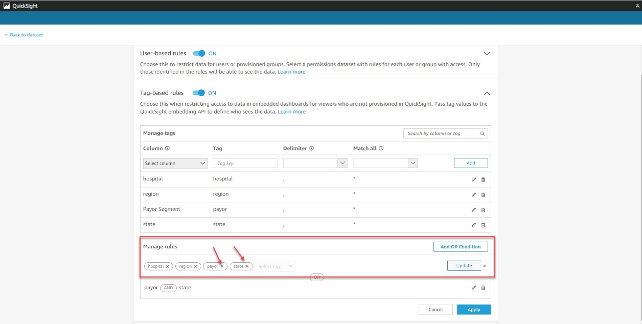
- Once the rules are created, choose Apply.

Set SessionTags
At runtime, when embedding the dashboards via the GenerateDahboardEmbedURLForAnonymousUser API, set SessionTags for each user.
SessionTags for NorthAdmin are as follows:
SessionTags for SouthAdmin are as follows:
SessionTags for PowerUser are as follows:
SessionTags for NorthMedicaidUser are as follows:
SessionTags for SouthMedicareUser are as follows:
The following screenshot shows what NorthMedicaidUser sees pertaining to all North hospitals in the East region and Medicaid in New York state.

The following screenshot shows what SouthMedicaidUser sees pertaining to all South hospitals in the South region or Medicare in all states.
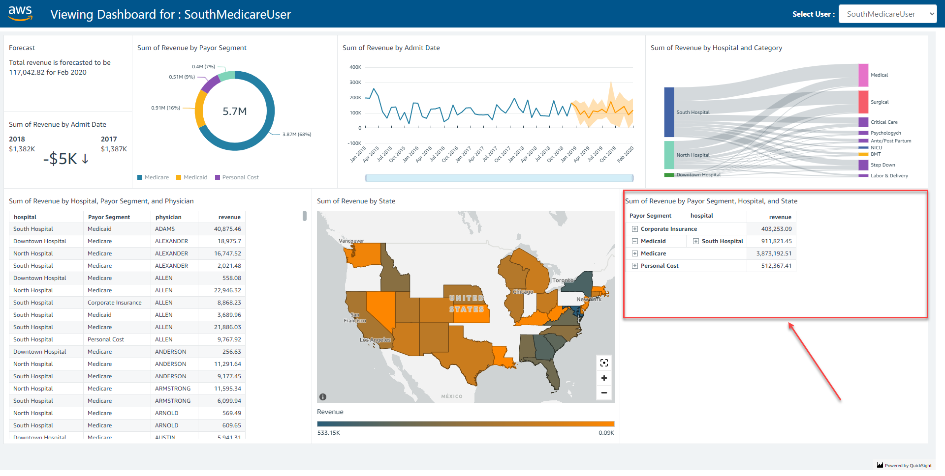
Based on session tags with OR of AND’s support, AnyHealth has secured data on the embedded dashboards such that each user only sees specific data based on their access. You can access the dashboard as one of the users (by changing the user on the drop-down menu on the top right) and see how the data changes based on the user selected.
Overall, with row-level security using OR of AND, AnyHealth is able to provide a compelling analytics experience within their SaaS application, while making sure that each user only sees the appropriate data without having to provision and manage users in QuickSight. QuickSight provides a highly scalable, secure analytics option that you can set up and roll out to production in days, instead of weeks or months previously.
Conclusion
The combination of embedding dashboards for users not provisioned in QuickSight and row-level security using tags with OR of AND enables developers and ISVs to quickly set up sophisticated, customized analytics for their application users—all without any infrastructure setup or user management, while scaling to millions of users. For more updates from QuickSight embedded analytics, see What’s New in the Amazon QuickSight User Guide.
If you have any questions or feedback, please leave a comment. For additional discussions and help getting answers to your questions, check out the QuickSight Community.
About the Authors
 Srikanth Baheti is a Specialized World Wide Principal Solution Architect for Amazon QuickSight. He started his career as a consultant and worked for multiple private and government organizations. Later he worked for PerkinElmer Health and Sciences & eResearch Technology Inc, where he was responsible for designing and developing high traffic web applications, highly scalable and maintainable data pipelines for reporting platforms using AWS services and Serverless computing.
 Raji Sivasubramaniam is a Sr. Solutions Architect at AWS, focusing on Analytics. Raji is specialized in architecting end-to-end Enterprise Data Management, Business Intelligence and Analytics solutions for Fortune 500 and Fortune 100 companies across the globe. She has in-depth experience in integrated healthcare data and analytics with wide variety of healthcare datasets including managed market, physician targeting and patient analytics.
 Mayank Agarwal is a product manager for Amazon QuickSight, AWS’ cloud-native, fully managed BI service. He focuses on embedded analytics and developer experience. He started his career as an embedded software engineer developing handheld devices. Prior to QuickSight he was leading engineering teams at Credence ID, developing custom mobile embedded device and web solutions using AWS services that make biometric enrollment and identification fast, intuitive, and cost-effective for Government sector, healthcare and transaction security applications.
This is a guest post by Joseph Landucci from BWH Hotels. In their own words, “BWH Hotels is a leading, global hospitality enterprise comprised of three hotel companies, including WorldHotels, Best Western Hotels & Resorts and SureStay Hotels. Our mission is to deliver trusted guest experiences, drive hotel success and foster a caring, inclusive culture that respects […]
Amazon Redshift is a widely used, fully managed, petabyte-scale cloud data warehouse. Tens of thousands of customers use Amazon Redshift to process exabytes of data every day to power their analytic workloads. Customers are looking for tools that make it easier to migrate from other data warehouses, such as Google BigQuery, to Amazon Redshift to take advantage of the service price-performance, ease of use, security, and reliability.
In this post, we show you how to use AWS native services to accelerate your migration from Google BigQuery to Amazon Redshift. We use AWS Glue, a fully managed, serverless, ETL (extract, transform, and load) service, and the Google BigQuery Connector for AWS Glue (for more information, refer to Migrating data from Google BigQuery to Amazon S3 using AWS Glue custom connectors). We also add automation and flexibility to simplify migration of multiple tables to Amazon Redshift using the Custom Auto Loader Framework.
Solution overview
The solution provides a scalable and managed data migration workflow to migrate data from Google BigQuery to Amazon Simple Storage Service (Amazon S3), and then from Amazon S3 to Amazon Redshift. This pre-built solution scales to load data in parallel using input parameters.
The following architecture diagram shows how the solution works. It starts with setting up the migration configuration to connect to Google BigQuery, then converts the database schemas, and finally migrates the data to Amazon Redshift.

The workflow contains the following steps:
- A configuration file is uploaded to an S3 bucket you have chosen for this solution. This JSON file contains the migration metadata, namely the following:
- A list of Google BigQuery projects and datasets.
- A list of all tables to be migrated for each project and dataset pair.
- An Amazon EventBridge rule triggers an AWS Step Functions state machine to start migrating the tables.
- The Step Functions state machine iterates on the tables to be migrated and runs an AWS Glue Python shell job to extract the metadata from Google BigQuery and store it in an Amazon DynamoDB table used for tracking the tables’ migration status.
- The state machine iterates on the metadata from this DynamoDB table to run the table migration in parallel, based on the maximum number of migration jobs without incurring limits or quotas on Google BigQuery. It performs the following steps:
- Runs the AWS Glue migration job for each table in parallel.
- Tracks the run status in the DynamoDB table.
- After the tables have been migrated, checks for errors and exits.
- The data exported from Google BigQuery is saved to Amazon S3. We use Amazon S3 (even though AWS Glue jobs can write directly to Amazon Redshift tables) for a few specific reasons:
- We can decouple the data migration and the data load steps.
- It offers more control on the load steps, with the ability to reload the data or pause the process.
- It provides fine-grained monitoring of the Amazon Redshift load status.
- The Custom Auto Loader Framework automatically creates schemas and tables in the target database and continuously loads data from Amazon S3 to Amazon Redshift.
A few additional points to note:
- If you have already created the target schema and tables in the Amazon Redshift database, you can configure the Custom Auto Loader Framework to not automatically detect and convert the schema.
- If you want more control over converting the Google BigQuery schema, you can use the AWS Schema Conversion Tool (AWS SCT). For more information, refer to Migrate Google BigQuery to Amazon Redshift using AWS Schema Conversion tool (SCT).
- As of this writing, neither the AWS SCT nor Custom Auto Loader Framework support the conversion of nested data types (record, array and struct). Amazon Redshift supports semistructured data using the Super data type, so if your table uses such complex data types, then you need to create the target tables manually.
To deploy the solution, there are two main steps:
- Deploy the solution stack using AWS CloudFormation.
- Deploy and configure Custom Auto Loader Framework to load files from Amazon S3 to Amazon Redshift.
Prerequisites
Before getting started, make sure you have the following:
- An account in Google Cloud, specifically a service account that has permissions to Google BigQuery.
- An AWS account with an AWS Identity and Access Management (IAM) user with an access key and secret key to configure the AWS Command Line Interface (AWS CLI). The IAM user also needs permissions to create an IAM role and policies.
- An Amazon Redshift cluster or Amazon Redshift Serverless workgroup. If you don’t have one, refer to Amazon Redshift Serverless.
- An S3 bucket. If you don’t want to use one of your existing buckets, you can create a new one. Note the name of the bucket to use later when you pass it to the CloudFormation stack as an input parameter.
- A configuration file with the list of tables to be migrated. This file should have the following structure:
Alternatively, you can download the demo file, which uses the open dataset created by the Centers for Medicare & Medicaid Services.
In this example, we named the file bq-mig-config.json
- Set up the Google BigQuery Connector for AWS Glue as described in the post Migrating data from Google BigQuery to Amazon S3 using AWS Glue custom connectors. The steps to consider are:
-
- Configure your Google account.
- Create an IAM role for AWS Glue (and note down the name of the IAM role).
- Subscribe to and activate the Google BigQuery Connector for AWS Glue.
Deploy the solution using AWS CloudFormation
To deploy the solution stack using AWS CloudFormation, complete the following steps:
- Choose Launch Stack:

This template provisions the AWS resources in the us-east-1 Region. If you want to deploy to a different Region, download the template bigquery-cft.yaml and launch it manually: on the AWS CloudFormation console, choose Create stack with new resources and upload the template file you downloaded.
The list of provisioned resources is as follows:
-
- An EventBridge rule to start the Step Functions state machine on the upload of the configuration file.
- A Step Functions state machine that runs the migration logic. The following diagram illustrates the state machine.

- An AWS Glue Python shell job used to extract the metadata from Google BigQuery. The metadata will be stored in an DynamoDB table, with a calculated attribute to prioritize the migration job. By default, the connector creates one partition per 400 MB in the table being read (before filtering). As of this writing, the Google BigQuery Storage API has a maximum quota for parallel read streams, so we set the limit for worker nodes for tables larger than 400 GB. We also calculate the max number of jobs that can run in parallel based on those values.
- An AWS Glue ETL job used to extract the data from each Google BigQuery table and saves it in Amazon S3 in Parquet format.
- A DynamoDB table (
bq\_to\_s3\_tracking) used to store the metadata for each table to be migrated (size of the table, S3 path used to store the migrated data, and the number of workers needed to migrate the table). - A DynamoDB table (
bq\_to\_s3\_maxstreams) used to store the maximum number of streams per state machine run. This helps us minimize job failures due to limits or quotas. Use the Cloud Formation template to customize the name of the DynamoDB table. The prefix for the DynamoDB table isbq\_to\_s3. - The IAM roles needed by the state machine and AWS Glue jobs.
- Choose Next.

- For Stack name, enter a name.
- For Parameters, enter the parameters listed in the following table, then choose Create.
| CloudFormation Template Parameter | Allowed Values | Description |
InputBucketName | S3 bucket name | The S3 bucket where the AWS Glue job stores the migrated data. The data will be actually stored in a folder named |
InputConnectionName | AWS Glue connection name, the default is glue-bq-connector-24 | The name of the AWS Glue connection that is created using the Google BigQuery connector. |
InputDynamoDBTablePrefix | DynamoDB table name prefix, the default is bq\_to\_s3 | The prefix that will be used when naming the two DynamoDB tables created by the solution. |
InputGlueETLJob | AWS Glue ETL job name, the default is bq-migration-ETL | The name you want to give to the AWS Glue ETL job. The actual script is saved in the S3 path specified in the parameter InputGlueS3Path. |
InputGlueMetaJob | AWS Glue Python shell job name, the default is bq-get-metadata | The name you want to give to AWS Glue Python shell job. The actual script is saved in the S3 path specified in the parameter InputGlueS3Path. |
InputGlueS3Path | S3 path, the default is s3://aws-glue-scripts-${AWS::Account}-${AWS::Region}/admin/ | This is the S3 path in which the stack will copy the scripts for AWS Glue jobs. Remember to replace: ${AWS::Account} with the actual AWS account ID and ${AWS::Region} with the Region you plan to use, or provide your own bucket and prefix in a complete path. |
InputMaxParallelism | Number of parallel migration jobs to run, the default is 30 | The maximum number of tables you want to migrate concurrently. |
InputBQSecret | AWS Secrets Manager secret name | The name of the AWS Secrets Manager secret in which you stored the Google BigQuery credential. |
InputBQProjectName | Google BigQuery project name | The name of your project in Google BigQuery in which you want to store temporary tables; you will need write permissions on the project. |
StateMachineName | Step Functions state machine name, the default is
| The name of the Step Functions state machine. |
SourceS3BucketName | S3 bucket name, the default is aws-blogs-artifacts-public | The S3 bucket where the artifacts for this post are stored. Do not change the default. |
Deploy and configure the Custom Auto Loader Framework to load files from Amazon S3 to Amazon Redshift
The Custom Auto Loader Framework utility makes data ingestion to Amazon Redshift simpler and automatically loads data files from Amazon S3 to Amazon Redshift. The files are mapped to the respective tables by simply dropping files into preconfigured locations on Amazon S3. For more details about the architecture and internal workflow, refer to Custom Auto Loader Framework.
To set up the Custom Auto Loader Framework, complete the following steps:
- Choose Launch Stack to deploy the CloudFormation stack in the
us-east-1Region:
- On the AWS CloudFormation console, choose Next.
- Provide the following parameters to help ensure the successful creation of resources. Make sure you have collected these values beforehand.
| Parameter Name | Allowed Values | Description |
|---|---|---|
CopyCommandSchedule | cron(0/5 * ? * * *) | The EventBridge rules KickoffFileProcessingSchedule and QueueRSProcessingSchedule are triggered based on this schedule. The default is 5 minutes. |
DatabaseName | dev | The Amazon Redshift database name. |
DatabaseSchemaName | public | The Amazon Redshift schema name. |
DatabaseUserName | demo | The Amazon Redshift user name who has access to run COPY commands on the Amazon Redshift database and schema. |
RedshiftClusterIdentifier | democluster | The Amazon Redshift cluster name. |
RedshiftIAMRoleARN | arn:aws:iam::7000000000:role/RedshiftDemoRole | The Amazon Redshift cluster attached role, which has access to the S3 bucket. This role is used in COPY commands. |
SourceS3Bucket | Your-bucket-name | The S3 bucket where data is located. Use the same bucket you used to store the migrated data as indicated in the previous stack. |
CopyCommandOptions | delimiter '|' gzip | Provide the additional COPY command data format parameters as follows:
|
InitiateSchemaDetection | Yes | The setting to dynamically detect the schema prior to file upload. |
The following screenshot shows an example of our parameters.
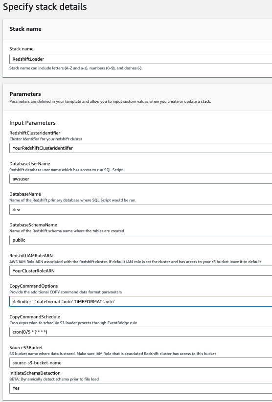
- Choose Create.
- Monitor the progress of the Stack creation and wait until it is complete.
- To verify the Custom Auto Loader Framework configuration, log in to the Amazon S3 console and navigate to the S3 bucket you provided as a value to the
SourceS3Bucketparameter.
You should see a new directory called s3-redshift-loader-source is created.
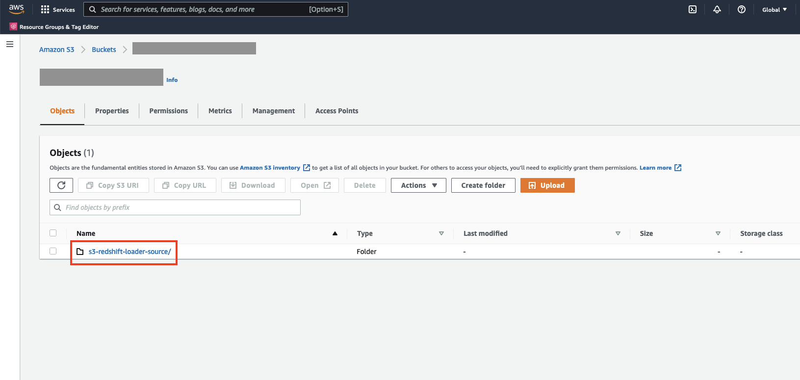
Test the solution
To test the solution, complete the following steps:
- Create the configuration file based on the prerequisites. You can also download the demo file.
- To set up the S3 bucket, on the Amazon S3 console, navigate to the folder
bq-mig-configin the bucket you provided in the stack. - Upload the config file into it.
- To enable EventBridge notifications to the bucket, open the bucket on the console and on the Properties tab, locate Event notifications.
- In the Amazon EventBridge section, choose Edit.
- Select On, then choose Save changes.

- On AWS Step Function console, monitor the run of the state machine.
- Monitor the status of the loads in Amazon Redshift. For instructions, refer to Viewing Current Loads.
- Open the Amazon Redshift Query Editor V2 and query your data.
Pricing considerations
You might have egress charges for migrating data out of Google BigQuery into Amazon S3. Review and calculate the cost for moving your data on your Google cloud billing console. As of this writing, AWS Glue 3.0 or later charges $0.44 per DPU-hour, billed per second, with a 1-minute minimum for Spark ETL jobs. For more information, see AWS Glue Pricing. With auto scaling enabled, AWS Glue automatically adds and removes workers from the cluster depending on the parallelism at each stage or microbatch of the job run.
Clean up
To avoid incurring future charges, clean up your resources:
- Delete the CloudFormation solution stack.
- Delete the CloudFormation Custom Auto Loader Framework stack.
Conclusion
In this post, we demonstrated how to build a scalable and automated data pipeline to migrate your data from Google BigQuery to Amazon Redshift. We also highlighted how the Custom Auto Loader framework can automate the schema detection, create tables for your S3 files, and continuously load the files into your Amazon Redshift warehouse. With this approach, you can automate the migration of entire projects (even multiple projects at the time) in Google BigQuery to Amazon Redshift. This helps improve data migration times into Amazon Redshift significantly through the automatic table migration parallelization.
The auto-copy feature in Amazon Redshift simplifies automatic data loading from Amazon S3 with a simple SQL command, users can easily automate data ingestion from Amazon S3 to Amazon Redshift using the Amazon Redshift auto-copy preview feature
For more information about the performance of the Google BigQuery Connector for AWS Glue, refer to Migrate terabytes of data quickly from Google Cloud to Amazon S3 with AWS Glue Connector for Google BigQuery and learn how to migrate a large amount of data (1.9 TB) into Amazon S3 quickly (about 8 minutes).
To learn more about AWS Glue ETL jobs, see Simplify data pipelines with AWS Glue automatic code generation and workflows and Making ETL easier with AWS Glue Studio.
About the Authors
 Tahir Aziz is an Analytics Solution Architect at AWS. He has worked with building data warehouses and big data solutions for over 13 years. He loves to help customers design end-to-end analytics solutions on AWS. Outside of work, he enjoys traveling and cooking.
 Ritesh Kumar Sinha is an Analytics Specialist Solutions Architect based out of San Francisco. He has helped customers build scalable data warehousing and big data solutions for over 16 years. He loves to design and build efficient end-to-end solutions on AWS. In his spare time, he loves reading, walking, and doing yoga.
 Fabrizio Napolitano is a Principal Specialist Solutions Architect for DB and Analytics. He has worked in the analytics space for the last 20 years, and has recently and quite by surprise become a Hockey Dad after moving to Canada.
 Manjula Nagineni is a Senior Solutions Architect with AWS based in New York. She works with major financial service institutions, architecting and modernizing their large-scale applications while adopting AWS Cloud services. She is passionate about designing big data workloads cloud-natively. She has over 20 years of IT experience in software development, analytics, and architecture across multiple domains such as finance, retail, and telecom.
 Sohaib Katariwala is an Analytics Specialist Solutions Architect at AWS. He has over 12 years of experience helping organizations derive insights from their data.
Apache Flink is a framework and distributed processing engine for stateful computations over data streams. Amazon Kinesis Data Analytics for Apache Flink is a fully managed service that enables you to use an Apache Flink application to process streaming data. The Deep Java Library (DJL) is an open-source, high-level, engine-agnostic Java framework for deep learning.
In this blog post, we demonstrate how you can use DJL within Kinesis Data Analytics for Apache Flink for real-time machine learning inference. Real-time inference can be valuable in a variety of applications and industries where it is essential to make predictions or take actions based on new data as quickly as possible with low latencies. We show how to load a pre-trained deep learning model from the DJL model zoo into a Flink job and apply the model to classify data objects in a continuous data stream. The DJL model zoo includes a wide variety of pre-trained models for image classification, semantic segmentation, speech recognition, text embedding generation, question answering, and more. It supports HuggingFace, Pytorch, MXNet, and TensorFlow model frameworks and also helps developers create and publish their own models. We will focus on image classification and use a popular classifier called ResNet-18 to produce predictions in real time. The model has been pre-trained on ImageNet with 1.2 million images belonging to 1,000 class labels.
We provide sample code, architecture diagrams, and an AWS CloudFormation template so you can follow along and employ ResNet-18 as your classifier to make real-time predictions. The solution we provide here is a powerful design pattern for continuously producing ML-based predictions on streaming data within Kinesis Data Analytics for Apache Flink. You can adapt the provided solution for your use case and choose an alternative model from the model zoo or even provide your own model.
Image classification is a classic problem that takes an image and selects the best-fitting class, such as whether the image from an autonomous driving system is that of a bicycle or a pedestrian. Common use cases for real-time inference on streams of images include classifying images from vehicle cameras and license plate recognition systems, and classifying images uploaded to social media and ecommerce websites. The use cases typically need low latency while handling high throughput and potentially bursty streams. For example, in ecommerce websites, real-time classification of uploaded images can help in marking pictures of banned goods or hazardous materials that have been supplied by sellers. Immediate determination through streaming inference is needed to trigger alerts and follow-up actions to prevent these images from being part of the catalog. This enables faster decision-making compared to batch jobs that run on a periodic basis. The data stream pipeline can involve multiple models for different purposes, such as classifying uploaded images into ecommerce categories of electronics, toys, fashion, and so on.
Solution overview
The following diagram illustrates the workflow of our solution.

The application performs the following steps:
- Read in images from Amazon Simple Storage Service (Amazon S3) using the Apache Flink Filesystem File Source connector.
- Window the images into a collection of records.
- Classify the batches of images using the DJL image classification class.
- Write inference results to Amazon S3 at the path specified.
Images are recommended to be of reasonable size so that they may fit into a Kinesis Processing Unit. Images larger than 50MB in size may result in latency in processing and classification.
The main class for this Apache Flink job is located at src/main/java/com.amazon.embeddedmodelinference/EMI.java. Here you can find the main() method and entry point to our Flink job.
Prerequisites
To get started, configure the following prerequisites on your local machine:
- Java 11 installed for local development of Apache Flink applications
- Maven downloaded and installed for packaging of Apache Flink applications
- Apache Flink set up on IntelliJ IDE on your local machine
Once this is set up, you can clone the code base to access the source code for this solution. The Java application code for this example is available on GitHub. To download the application code, clone the remote repository using the following command:
Find and navigate to the folder of the image classification example, called image-classification.
An example set of images to stream and test the code is available in the imagenet-sample-images folder.
Let’s walk through the code step by step.
Test on your local machine
If you would like to test this application locally on your machine, ensure you have AWS credentials set up locally on your machine. Additionally, download the Flink S3 Filesystem Hadoop JAR to use with your Apache Flink installation and place it in a folder named plugins/s3 in the root of your project. Then configure the following environment variables either on your IDE or in your machine’s local variable scope:
Replace these values with your own.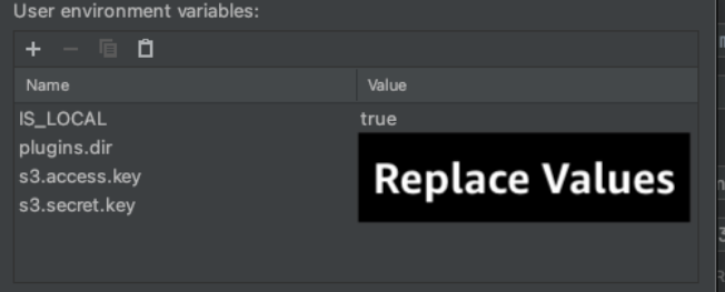
After configuring the environment variables and downloading the necessary plugin JAR, let’s look at the code.
In the main method, after setting up our StreamExecutionEnvironment, we define our FileSource to read files from Amazon S3. By default, this source operator reads from a sample bucket. You can replace this bucket name with your own by changing the variable called bucket, or setting the application property on Kinesis Data Analytics for Apache Flink once deployed.
The FileSource is configured to read in files in the ImageReaderFormat, and will check Amazon S3 for new images every 10 seconds. This can be configured as well.
After we have read in our images, we convert our FileSource into a stream that can be processed:
Next, we create a tumbling window of a variable time window duration, specified in the configuration, defaulting to 60 seconds. Every window close creates a batch (list) of images to be classified using a ProcessWindowFunction.
This ProcessWindowFunction calls the classifier predict function on the list of images and returns the best probability of classification from each image. This result is then sent back to the Flink operator, where it’s promptly written out to the S3 bucket path of your configuration.
In Classifier.java, we read the image and apply crop, transpose, reshape, and finally convert to an N-dimensional array that can be processed by the deep learning model. Then we feed the array to the model and apply a forward pass. During the forward pass, the model computes the neural network layer by layer. At last, the output object contains the probabilities for each image object that the model is being trained on. We map the probabilities with the object name and return to the map function.
Deploy the solution with AWS CloudFormation
To run this code base on Kinesis Data Analytics for Apache Flink, we have a helpful CloudFormation template that will spin up the necessary resources. Simply open AWS CloudShell or your local machine’s terminal and enter the following commands. Complete the following steps to deploy the solution:
- If you don’t have the AWS Cloud Development Kit (AWS CDK) bootstrapped in your account, run the following command, providing your account number and current Region:
The script will clone a GitHub repo of images to classify and upload them to your source S3 bucket. Then it will launch the CloudFormation stack given your input parameters. 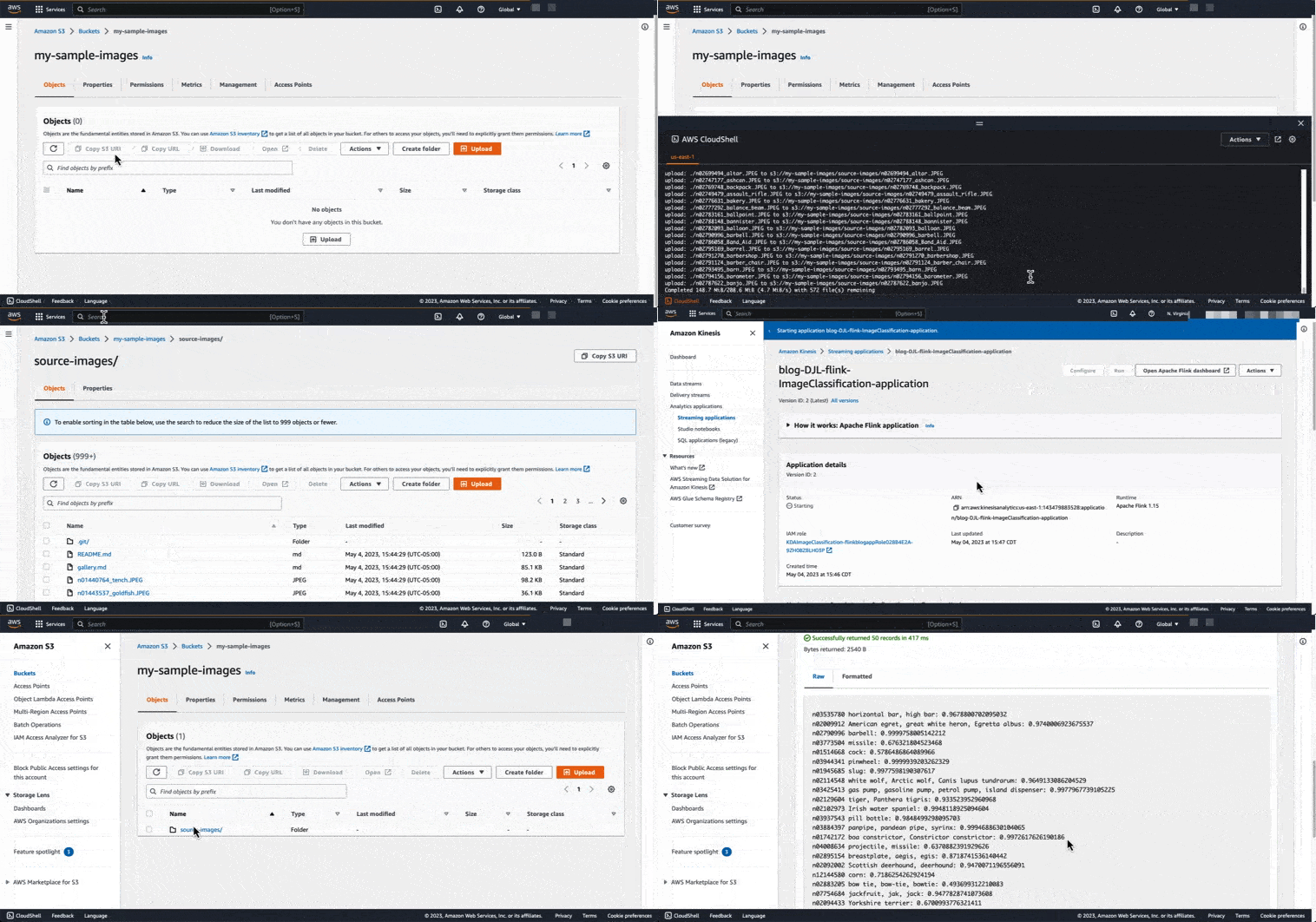
- Enter the following code and replace the BUCKET variables with your own source bucket and sink bucket, which will contain the source images and the classifications, respectively:
This CloudFormation stack creates the following resources:
-
- A Kinesis Data Analytics application with 1 Kinesis Processing Unit (KPU) preconfigured with some application properties
-
- An S3 bucket for your output results
-
- AWS Identity and Access Management (IAM) roles for the communication between the two services
- When the stack is complete, navigate to the Kinesis Data Analytics for Apache Flink console.
- Find the application called
blog-DJL-flink-ImageClassification-applicationand choose Run. - On the Amazon S3 console, navigate to the bucket you specified in the
outputBucketPathvariable.
If you have readable images in the source bucket listed, you should see classifications of those images within the checkpoint interval of the running application.
Deploy the solution manually
If you prefer to use your own code base, you can follow the manual steps in this section:
- After you clone the application locally, create your application JAR by navigating to the directory that contains your
pom.xmland running the following command:
This builds your application JAR in the target/ directory called embedded-model-inference-1.0-SNAPSHOT.jar.
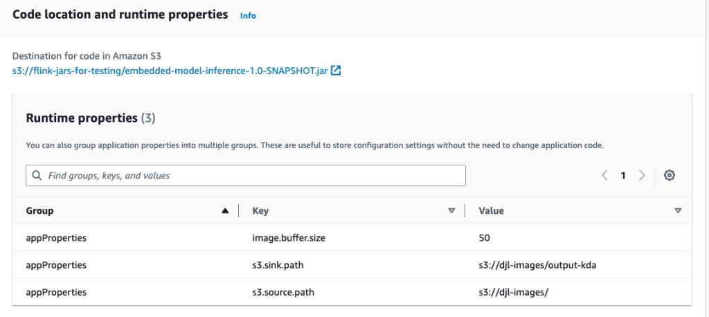
- Upload this application JAR to an S3 bucket, either the one created from the CloudFormation template, or another one to store code artifacts.
- You can then configure your Kinesis Data Analytics application to point to this newly uploaded S3 JAR file.
- This is also a great opportunity to configure your runtime properties, as shown in the following screenshot.
- Choose Run to start your application.
You can open the Apache Flink Dashboard to check for application exceptions or to see data flowing through the tasks defined in the code.

Validate the results
To validate our results, let’s check the results in Amazon S3 by navigating to the Amazon S3 console and finding our S3 bucket. We can find the output in a folder called output-kda.

When we choose one of the data-partitioned folders, we can see partition files. Ensure that there is no underscore in front of your part file, because this indicates that the results are still being finalized according to the rollover interval defined in Apache Flink’s FileSink connector. After the underscores have disappeared, we can use Amazon S3 Select to view our data.

We now have a solution that continuously performs classification on incoming images in real time using Kinesis Data Analytics for Apache Flink. It extracts a pre-trained classification model (ResNet-18) from the DJL model zoo, applies some preprocessing, loads the model into a Flink operator’s memory, and continuously applies the model for online predictions on streaming images.
Although we used ResNet-18 in this post, you can choose another model by modifying the classifier. The DJL model zoo provides many other models, both for classification and other applications, that can be used out of the box. You can also load your custom model by providing an S3 link or URL to the criteria. DJL supports models in a large number of engines such as PyTorch, ONNX, TensorFlow, and MXNet. Using a model in the solution is relatively simple. All of the preprocessing and postprocessing code is encapsulated in the (built-in) translator, so all we have to do is load the model, create a predictor, and call predict(). This is done within the data source operator, which processes the stream of input data and sends the links to the data to the inference operator where the model you selected produces the prediction. Then the sink operator writes the results.
The CloudFormation template in this example focused on a simple 1 KPU application. You could extend the solution to further scale out to large models and high-throughput streams, and support multiple models within the pipeline.
Clean up
To clean up the CloudFormation script you launched, complete the following steps:
- Empty the source bucket you specified in the bash script.
- On the AWS CloudFormation console, locate the CloudFormation template called
KDAImageClassification. - Delete the stack, which will remove all of the remaining resources created for this post.
- You may optionally delete the bootstrapping CloudFormation template,
CDKToolkit, which you launched earlier as well.
Conclusion
In this post, we presented a solution for real-time classification using the Deep Java Library within Kinesis Data Analytics for Apache Flink. We shared a working example and discussed how you can adapt the solution for your specific ML use case. If you have any feedback or questions, please leave them in the comments section.
About the Authors
 Jeremy Ber has been working in the telemetry data space for the past 9 years as a Software Engineer, Machine Learning Engineer, and most recently a Data Engineer. At AWS, he is a Streaming Specialist Solutions Architect, supporting both Amazon Managed Streaming for Apache Kafka (Amazon MSK) and AWS’s managed offering for Apache Flink.
 Deepthi Mohan is a Principal Product Manager for Amazon Kinesis Data Analytics, AWS’s managed offering for Apache Flink.
 Gaurav Rele is a Data Scientist at the Amazon ML Solution Lab, where he works with AWS customers across different verticals to accelerate their use of machine learning and AWS Cloud services to solve their business challenges.
Amazon OpenSearch Service is a fully open-source search and analytics engine that securely unlocks real-time search, monitoring, and analysis of business and operational data for use cases like recommendation engines, ecommerce sites, and catalog search. To be successful in your business, you need your systems to be highly available and performant, minimizing downtime and avoiding failure. When you use OpenSearch Service as your primary means of monitoring your infrastructure, you need to ensure its availability as well. Downtime for OpenSearch Service can have a significant effect on your business outcomes, such as loss of revenue, loss in productivity, loss in brand value, and more.
The industry standard for measuring availability is class of nines. OpenSearch Service provides 3 9’s of availability, when you follow best practices, which means it guarantees less than 43.83 minutes of downtime a month. In this post, you will learn how you can configure your OpenSearch Service domain for high availability and performance by following best practices and recommendations while setting up your domain.
There are two essential elements that influence your domain’s availability: the resource utilization of your domain, which is mostly driven by your workload, and external events such as infrastructure failures. Although the former can be controlled through continuous monitoring of the domain’s performance and health and scaling the domain accordingly, the latter cannot. To mitigate the impact of external events such as an Availability Zone outage, instance or disk failure, or networking issues on your domain, you must provision additional capacity, distributed over multiple Availability Zones, and keep multiple copies of data. Failure to do so may result in degraded performance, unavailability, and, in the worst-case situation, data loss.
Let’s look at the options available to you to ensure that domain is available and performant.
Cluster configuration
Under this section we will talk about various configuration options you have to setup your cluster properly which includes specifying the number of AZ for the deployment, setting up the master and data nodes, setting up indexes and shards.
Multi-AZ deployment
Data nodes are responsible for processing indexing and search requests in your domain. Deploying your data nodes across multiple Availability Zones improves the availability of your domain by adding redundant, per-zone data storage and processing. With a Multi-AZ deployment, your domain can remain available even when a full Availability Zone becomes unavailable. For production workloads, AWS recommends using three Availability Zones for your domain. Use two Availability Zones for Regions that support only two for improved availability. This ensures that your domain is available in the event of a Single-AZ failure.
Dedicated cluster manager (master nodes)
AWS recommends using three dedicated cluster manager (CM) nodes for all production workloads. CM nodes track the cluster’s health, the state and location of its indexes and shards, the mapping for all the indexes, and the availability of its data nodes, and it maintains a list of cluster-level tasks in process. Without dedicated CM nodes, the cluster uses data nodes, which makes the cluster vulnerable to workload demands. You should size CM nodes based on the size of the task—primarily, the data node counts, the index counts, and the shard counts. OpenSearch Service always deploys CM nodes across three Availability Zones, when supported by the Region (two in one Availability Zones and one in other Availability Zones if regions have only two Availability Zones). For a running domain, only one of the three CM nodes works as an elected leader. The other two CM nodes participate in an election if the elected CM node fails.
The following table shows AWS’s recommendations for CM sizing. CM nodes do work based on the number of nodes, indexes, shards, and mapping. The more work, the more compute and memory you need to hold and work with the cluster state.
| Instance Count | Cluster Manager Node RAM Size | Maximum Supported Shard Count | Recommended Minimum Dedicated Cluster Manager Instance Type |
| 1–10 | 8 GiB | 10,000 | m5.large.search or m6g.large.search |
| 11–30 | 16 GiB | 30,000 | c5.2xlarge.search or c6g.2xlarge.search |
| 31–75 | 32 GiB | 40,000 | c5.4xlarge.search or c6g.4xlarge.search |
| 76 – 125 | 64 GiB | 75,000 | r5.2xlarge.search or r6g.2xlarge.search |
| 126 – 200 | 128 GiB | 75,000 | r5.4xlarge.search or r6g.4xlarge.search |
Indexes and shards
Indexes are a logical construct that houses a collection of documents. You partition your index for parallel processing by specifying a primary shard count, where shards represent a physical unit for storing and processing data. In OpenSearch Service, a shard can be either a primary shard or a replica shard. You use replicas for durability—if the primary shard is lost, OpenSearch Service promotes one of the replicas to primary—and for improving search throughput. OpenSearch Service ensures that the primary and replica shards are placed in different nodes and across different Availability Zones, if deployed in more than one Availability Zone. For high availability, AWS recommends configuring at least two replicas for each index in a three-zone setup to avoid disruption in performance and availability. In a Multi-AZ setup, if a node fails or in the rare worst case an Availability Zone fails, you will still have a copy of the data.
Cluster monitoring and management
As discussed earlier, selecting your configuration based on best practices is only half the job. We also need to continuously monitor the resource utilization and performance to determine if the domain needs to be scaled. An under-provisioned or over-utilized domain can result in performance degradation and eventually unavailability.
CPU utilization
You use the CPU in your domain to run your workload. As a general rule, you should target 60% average CPU utilization for any data node, with peaks at 80%, and tolerate small spikes to 100%. When you consider availability, and especially considering the unavailability of a full zone, there are two scenarios. If you have two Availability Zones, then each zone handles 50% of the traffic. If a zone becomes unavailable, the other zone will take all of that traffic, doubling CPU utilization. In that case, you need to be at around 30–40% average CPU utilization in each zone to maintain availability. If you are running three Availability Zones, each zone is taking 33% of the traffic. If a zone becomes unavailable, each other zone will gain approximately 17% traffic. In this case, you should target 50–60% average CPU utilization.
Memory utilization
OpenSearch Service supports two types of garbage collection. The first is G1 garbage collection (G1GC), which is used by OpenSearch Service nodes, powered by AWS Graviton 2. The second is Concurrent Mark Sweep (CMS), which is used by all nodes powered by other processors. Out of all the memory allocated to a node, half of the memory (up to 32 GB) is assigned to the Java heap, and the rest of the memory is used by other operating system tasks, the file system cache, and so on. To maintain availability for a domain, we recommend keeping the max JVM utilization at around 80% in CMS and 95% in G1GC. Anything beyond that would impact the availability of your domain and make your cluster unhealthy. We also recommend enabling auto-tune, which actively monitors the memory utilization and triggers the garbage collector.
Storage utilization
OpenSearch Service publishes several guidelines for sizing of domains. We provide an empirical formula so that you can determine the right amount of storage required for your requirements. However, it’s important to keep an eye out for the depletion of storage with time and changes in workload characteristics. To ensure the domain doesn’t run out of storage and can continue to index data, you should configure Amazon CloudWatch alarms and monitor your free storage space.
AWS also recommends choosing a primary shard count so that each shard is within an optimal size band. You can determine the optimal shard size through proof-of-concept testing with your data and traffic. We use 10–30 GB primary shard sizes for search use cases and 45–50 GB primary shard sizes for log analytics use cases as a guideline. Because shards are the workers in your domain, they are directly responsible for the distribution of the workload across the data nodes. If your shards are too large, you may see stress in your Java heap from large aggregations, worse query performance, and worse performance on cluster-level tasks like shard rebalancing, snapshots, and hot-to-warm migrations. If your shards are too small, they can overwhelm the domain’s Java heap space, worsen query performance through excessive internal networking, and make cluster-level tasks slow. We also recommend keeping the number of shards per node proportional to the heap available (half of the instance’s RAM up to 32 GB)—25 shards per GB of Java heap. This makes a practical limit of 1,000 shards on any data node in your domain.
Conclusion
In this post, you learned various tips and tricks to set up a highly available domain using OpenSearch Service, which helps you to keep OpenSearch Service performant and available by running it across three Availability Zones.
Stay tuned for a series of posts focusing on the various features and functionalities with OpenSearch Service. If you have feedback about this post, submit it in the comments section. If you have questions about this post, start a new thread on the OpenSearch Service forum or contact AWS Support.
About the authors
 Rohin Bhargava is a Sr. Product Manager with the Amazon OpenSearch Service team. His passion at AWS is to help customers find the correct mix of AWS services to achieve success for their business goals.
 Prashant Agrawal is a Sr. Search Specialist Solutions Architect with Amazon OpenSearch Service. He works closely with customers to help them migrate their workloads to the cloud and helps existing customers fine-tune their clusters to achieve better performance and save on cost. Before joining AWS, he helped various customers use OpenSearch and Elasticsearch for their search and log analytics use cases. When not working, you can find him traveling and exploring new places. In short, he likes doing Eat → Travel → Repeat.
This is a guest post by Brian Kasen and Rebecca McAlpine from Trakstar, now a part of Mitratech.
Trakstar, now a part of Mitratech, is a human resources (HR) software company that serves customers from small businesses and educational institutions to large enterprises, globally. Trakstar supercharges employee performance around pivotal moments in talent development. Our team focuses on helping HR leaders make smarter decisions to attract, retain, and engage their workforce. Trakstar has been used by HR leaders for over 20 years, specifically in the areas of applicant tracking, performance management, and learning management.
In 2023, Trakstar joined Mitratech’s world-class portfolio of Human Resources and Compliance products. This includes complementary solutions for OFCCP compliance management; diversity, equity, and inclusion (DEI) strategy and recruiting (now with Circa); advanced background screening; I-9 compliance; workflow automation; policy management; and more.
In 2022, Trakstar launched what is now called Trakstar Insights, which unlocks new analytical insights for HR across the employee life cycle. It’s powered by Amazon QuickSight, a cloud-native business intelligence (BI) tool that enables embedded customized, interactive visuals and dashboards within the product experience.
In this post, we discuss how we use QuickSight to deliver powerful HR analytics to over 3,000 customers and 43,000 users while forecasting savings of 84% year-over-year as compared to our legacy reporting solutions.
The evolving HR landscape
Over the past few years, new realities have emerged, creating unfamiliar challenges for businesses and new opportunities for HR leaders. In 2020, new working arrangements spawned by immediate necessity, with many companies shifting to fully remote or hybrid setups for the first time. As we still adapt to this new environment, organizations have trouble finding talent, with record-level resignation rates and a tight labor market.
As companies look to combat these new challenges, we’ve seen the rise of the Chief People Officer because organizations now recognize people as their greatest asset. With our three products, Trakstar Hire, Trakstar Perform, and Trakstar Learn, HR leaders can use data to take an integrated approach and foster a better employee experience.
Choosing QuickSight to bring solutions to the new reality of work
To help HR leaders navigate the new challenges of our time and answer new questions, we decided to embed interactive dashboards directly into each Trakstar product focused on the growing area of people analytics. QuickSight allowed us to meet our customers’ needs quickly and played a key role in our overall analytics strategy. Because QuickSight is fully managed and serverless, we were able to focus on building value for customers and develop an embedded dashboard delivery solution to support all three products, rather than focusing on managing and optimizing infrastructure. QuickSight allowed us to focus on building dashboards that address key pain points for customers and rapidly innovate.
In a 12-month timespan, we designed and launched five workforce dashboards to over 20,000 users, spanning hiring, performance, learning, and peer group benchmarking. During the same 12-month time period, in addition to our Trakstar Insights dashboard releases, we also migrated Trakstar Learn’s legacy reporting to QuickSight, which supports an additional 20,000 users.

Delighting our customers by embedding QuickSight
Our goal was to build something that would delight our customers by making a material difference in their daily lives. We set out to create something that went beyond a typical Minimum Viable Product, but rather create a Minimum Lovable Product. By this, we mean delivering something that would make the most significant difference for customers in the shortest time possible.
We used QuickSight to build a curated dashboard that went beyond traditional dashboards of bar charts and tables. Our dashboards present retention trends, hiring trends, and learning outcomes supplemented with data narratives that empower our customers to easily interpret trends and make data-driven decisions.
In January 2022, we launched the Perform Insights dashboards. This enabled our customers to see their data in a way they had never seen before. With this dashboard, HR leaders can compare organizational strengths and weaknesses over time. The power of QuickSight lets our customers slice and dice the data in different ways. As shown in the following screenshot, customers can filter by Review Process Type or Group Type and then take actionable next steps based on data. They can see where top and bottom performers reside within teams and take steps to retain top performers and address lower-performing employees. These were net new analytics for our HR customers.

Our investment in building with QuickSight was quickly validated just days after launch. One of our sales reps was able to engage a lost opportunity and land a multi-year contract for double our typical average contract value. We followed up our first dashboard launch by expanding Trakstar Insights into our other products with the Learning Insights dashboard for Trakstar Learn and Hiring Insights for Trakstar Hire (see the following screenshots). These dashboards provided new lenses into how customers can look at their recruitment and training data.


Through our benchmarking dashboards, we empowered our customers so they can now compare their trends against other Trakstar customers in the same industry or of similar size, as shown in the following screenshots. These benchmarking dashboards can help our customers answer the “Am I normal?” question when it comes to talent acquisition and other areas.


Telling a story with people data for reporting
With the custom narrative visual type in QuickSight, our benchmarking dashboards offer dynamic, customer-specific interpretations of their trends and do the heavy lifting interpretation for them while providing action-oriented recommendations. The burden of manual spreadsheet creation, manual export, data manipulation, and analysis has been eliminated for our customers. They can now simply screenshot sections from the dashboards, drop them into a slide deck, and then speak confidently with their executive teams on what the trends mean for their organization, thereby saving tremendous time and effort and opening the door for new opportunities.
A Trakstar Hire customer shared with us, “You literally just changed my life. I typically spend hours creating slides, and this is the content—right here, ready to screenshot for my presentations!”
Building on our success with QuickSight
With the success of launching Trakstar Insights with QuickSight, we knew we could modernize the reporting functionality in Trakstar Learn by migrating to QuickSight from our legacy embedded BI vendor. Our legacy solution was antiquated and expensive. QuickSight brings a more cohesive and modern look to reporting at a significantly lower overall cost. With the session-based pricing model in QuickSight, we are projecting to save roughly 84% this year while offering customers a more powerful analytics experience.

Summary
Building with QuickSight has helped us thrive by delivering valuable HR solutions to our customers. We are excited to continue innovating with QuickSight to deliver even more value to our customers.
To learn more about how you can embed customized data visuals and interactive dashboards into any application, visit Amazon QuickSight Embedded.
About the authors:
 Brian Kasen is the Director, Business Intelligence at Mitratech. He is passionate about helping HR leaders be more data-driven in their efforts to hire, retain, and engage their employees. Prior to Mitratech, Brian spent much of his career building analytic solutions across a range of industries, including higher education, restaurant, and software.
 Rebecca McAlpine is the Senior Product Manager for Trakstar Insights at Mitratech. Her experience in HR tech experience has allowed her to work in various areas, including data analytics, business systems optimization, candidate experience, job application management, talent engagement strategy, training, and performance management.
Customers have been using data warehousing solutions to perform their traditional analytics tasks. Recently, data lakes have gained lot of traction to become the foundation for analytical solutions, because they come with benefits such as scalability, fault tolerance, and support for structured, semi-structured, and unstructured datasets.
Data lakes are not transactional by default; however, there are multiple open-source frameworks that enhance data lakes with ACID properties, providing a best of both worlds solution between transactional and non-transactional storage mechanisms.
Traditional batch ingestion and processing pipelines that involve operations such as data cleaning and joining with reference data are straightforward to create and cost-efficient to maintain. However, there is a challenge to ingest datasets, such as Internet of Things (IoT) and clickstreams, at a fast rate with near-real-time delivery SLAs. You will also want to apply incremental updates with change data capture (CDC) from the source system to the destination. To make data-driven decisions in a timely manner, you need to account for missed records and backpressure, and maintain event ordering and integrity, especially if the reference data also changes rapidly.
In this post, we aim to address these challenges. We provide a step-by-step guide to join streaming data to a reference table changing in real time using AWS Glue, Amazon DynamoDB, and AWS Database Migration Service (AWS DMS). We also demonstrate how to ingest streaming data to a transactional data lake using Apache Hudi to achieve incremental updates with ACID transactions.
Solution overview
For our example use case, streaming data is coming through Amazon Kinesis Data Streams, and reference data is managed in MySQL. The reference data is continuously replicated from MySQL to DynamoDB through AWS DMS. The requirement here is to enrich the real-time stream data by joining with the reference data in near-real time, and to make it queryable from a query engine such as Amazon Athena while keeping consistency. In this use case, reference data in MySQL can be updated when the requirement is changed, and then queries need to return results by reflecting updates in the reference data.
This solution addresses the issue of users wanting to join streams with changing reference datasets when the size of the reference dataset is small. The reference data is maintained in DynamoDB tables, and the streaming job loads the full table into memory for each micro-batch, joining a high-throughput stream to a small reference dataset.
The following diagram illustrates the solution architecture.

Prerequisites
For this walkthrough, you should have the following prerequisites:
- An AWS account.
- A host with the installed MySQL utility, such as an Amazon Elastic Compute Cloud (Amazon EC2) instance, AWS Cloud9, your laptop, and so on. The host is used to access an Amazon Aurora MySQL-Compatible Edition cluster that you create and to run a Python script that sends sample records to the Kinesis data stream.
Create IAM roles and S3 bucket
In this section, you create an Amazon Simple Storage Service (Amazon S3) bucket and two AWS Identity and Access Management (IAM) roles: one for the AWS Glue job, and one for AWS DMS. We do this using an AWS CloudFormation template. Complete the following steps:
- Sign in to the AWS CloudFormation console.
- Choose Launch Stack::

- Choose Next.
- For Stack name, enter a name for your stack.
- For DynamoDBTableName, enter
tgt\_country\_lookup\_table. This is the name of your new DynamoDB table. - For S3BucketNamePrefix, enter the prefix of your new S3 bucket.
- Select I acknowledge that AWS CloudFormation might create IAM resources with custom names.
- Choose Create stack.
Stack creation can take about 1 minute.
Create a Kinesis data stream
In this section, you create a Kinesis data stream:
- On the Kinesis console, choose Data streams in the navigation pane.
- Choose Create data stream.
- For Data stream name, enter your stream name.
- Leave the remaining settings as default and choose Create data stream.
A Kinesis data stream is created with on-demand mode.
Create and configure an Aurora MySQL cluster
In this section, you create and configure an Aurora MySQL cluster as the source database. First, configure your source Aurora MySQL database cluster to enable CDC through AWS DMS to DynamoDB.
Create a parameter group
Complete the following steps to create a new parameter group:
- On the Amazon RDS console, choose Parameter groups in the navigation pane.
- Choose Create parameter group.
- For Parameter group family, select
aurora-mysql5.7. - For Type, choose DB Cluster Parameter Group.
- For Group name, enter
my-mysql-dynamodb-cdc. - For Description, enter
Parameter group for demo Aurora MySQL database. - Choose Create.
- Select
my-mysql-dynamodb-cdc, and choose Edit under Parameter group actions. - Edit the parameter group as follows:
| Name | Value |
| binlog\_row\_image | full |
| binlog\_format | ROW |
| binlog\_checksum | NONE |
| log\_slave\_updates | 1 |
- Choose Save changes.

Create the Aurora MySQL cluster
Complete following steps to create the Aurora MySQL cluster:
- On the Amazon RDS console, choose Databases in the navigation pane.
- Choose Create database.
- For Choose a database creation method, choose Standard create.
- Under Engine options, for Engine type, choose Aurora (MySQL Compatible).
- For Engine version, choose Aurora (MySQL 5.7) 2.11.2.
- For Templates, choose Production.
- Under Settings, for DB cluster identifier, enter a name for your database.
- For Master username, enter your primary user name.
- For Master password and Confirm master password, enter your primary password.
- Under Instance configuration, for DB instance class, choose Burstable classes (includes t classes) and choose db.t3.small.
- Under Availability & durability, for Multi-AZ deployment, choose Don’t create an Aurora Replica.
- Under Connectivity, for Compute resource, choose Don’t connect to an EC2 compute resource.
- For Network type, choose IPv4.
- For Virtual private cloud (VPC), choose your VPC.
- For DB subnet group, choose your public subnet.
- For Public access, choose Yes.
- For VPC security group (firewall), choose the security group for your public subnet.
- Under Database authentication, for Database authentication options, choose Password authentication.
- Under Additional configuration, for DB cluster parameter group, choose the cluster parameter group you created earlier.
- Choose Create database.
Grant permissions to the source database
The next step is to grant the required permission on the source Aurora MySQL database. Now you can connect to the DB cluster using the MySQL utility. You can run queries to complete the following tasks:
- Create a demo database and table and run queries on the data
- Grant permission for a user used by the AWS DMS endpoint
Complete the following steps:
- Log in to the EC2 instance that you’re using to connect to your DB cluster.
- Enter the following command at the command prompt to connect to the primary DB instance of your DB cluster:
- Run the following SQL command to create a database:
- Run the following SQL command to create a table:
- Run the following SQL command to populate the table with data:
- Run the following SQL command to create a user for the AWS DMS endpoint and grant permissions for CDC tasks (replace the placeholder with your preferred password):
Create and configure AWS DMS resources to load data into the DynamoDB reference table
In this section, you create and configure AWS DMS to replicate data into the DynamoDB reference table.
Create an AWS DMS replication instance
First, create an AWS DMS replication instance by completing the following steps:
- On the AWS DMS console, choose Replication instances in the navigation pane.
- Choose Create replication instance.
- Under Settings, for Name, enter a name for your instance.
- Under Instance configuration, for High Availability, choose Dev or test workload (Single-AZ).
- Under Connectivity and security, for VPC security groups, choose default.
- Choose Create replication instance.
Create Amazon VPC endpoints
Optionally, you can create Amazon VPC endpoints for DynamoDB when you need to connect to your DynamoDB table from the AWS DMS instance in a private network. Also make sure that you enable Publicly accessible when you need to connect to a database outside of your VPC.
Create an AWS DMS source endpoint
Create an AWS DMS source endpoint by completing the following steps:
- On the AWS DMS console, choose Endpoints in the navigation pane.
- Choose Create endpoint.
- For Endpoint type, choose Source endpoint.
- Under Endpoint configuration, for Endpoint identifier, enter a name for your endpoint.
- For Source engine, choose Amazon Aurora MySQL.
- For Access to endpoint database, choose Provide access information manually.
- For Server Name, enter the endpoint name of your Aurora writer instance (for example,
mycluster.cluster-123456789012.us-east-1.rds.amazonaws.com). - For Port, enter
3306. - For User name, enter a user name for your AWS DMS task.
- For Password, enter a password.
- Choose Create endpoint.
Crate an AWS DMS target endpoint
Create an AWS DMS target endpoint by completing the following steps:
- On the AWS DMS console, choose Endpoints in the navigation pane.
- Choose Create endpoint.
- For Endpoint type, choose Target endpoint.
- Under Endpoint configuration, for Endpoint identifier, enter a name for your endpoint.
- For Target engine, choose Amazon DynamoDB.
- For Service access role ARN, enter the IAM role for your AWS DMS task.
- Choose Create endpoint.
Create AWS DMS migration tasks
Create AWS DMS database migration tasks by completing the following steps:
- On the AWS DMS console, choose Database migration tasks in the navigation pane.
- Choose Create task.
- Under Task configuration, for Task identifier, enter a name for your task.
- For Replication instance, choose your replication instance.
- For Source database endpoint, choose your source endpoint.
- For Target database endpoint, choose your target endpoint.
- For Migration type, choose Migrate existing data and replicate ongoing changes.
- Under Task settings, for Target table preparation mode, choose Do nothing.
- For Stop task after full load completes, choose Don’t stop.
- For LOB column settings, choose Limited LOB mode.
- For Task logs, enable Turn on CloudWatch logs and Turn on batch-optimized apply.
- Under Table mappings, choose JSON Editor and enter the following rules.
Here you can add values to the column. With the following rules, the AWS DMS CDC task will first create a new DynamoDB table with the specified name in target-table-name. Then it will replicate all the records, mapping the columns in the DB table to the attributes in the DynamoDB table.

- Choose Create task.
Now the AWS DMS replication task has been started.
- Wait for the Status to show as Load complete.
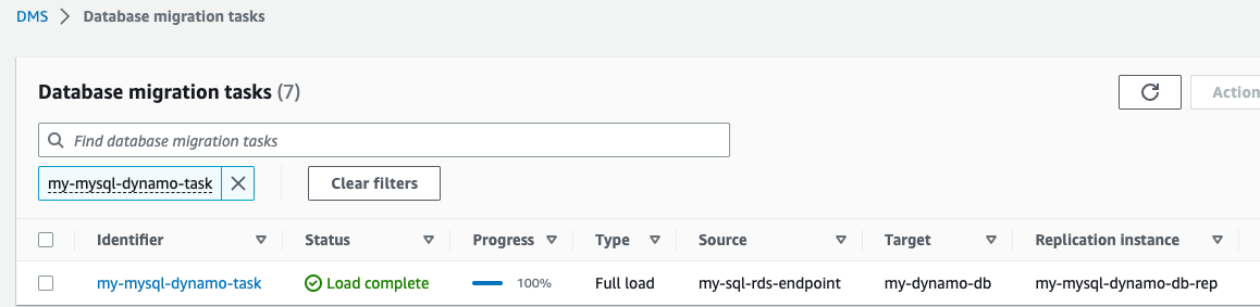
- On the DynamoDB console, choose Tables in the navigation pane.
- Select the DynamoDB reference table, and choose Explore table items to review the replicated records.
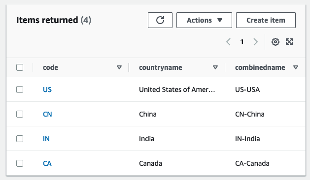
Create an AWS Glue Data Catalog table and an AWS Glue streaming ETL job
In this section, you create an AWS Glue Data Catalog table and an AWS Glue streaming extract, transform, and load (ETL) job.
Create a Data Catalog table
Create an AWS Glue Data Catalog table for the source Kinesis data stream with the following steps:
- On the AWS Glue console, choose Databases under Data Catalog in the navigation pane.
- Choose Add database.
- For Name, enter
my\_kinesis\_db. - Choose Create database.
- Choose Tables under Databases, then choose Add table.
- For Name, enter
my\_stream\_src\_table. - For Database, choose
my\_kinesis\_db. - For Select the type of source, choose Kinesis.
- For Kinesis data stream is located in, choose my account.
- For Kinesis stream name, enter a name for your data stream.
- For Classification, select JSON.
- Choose Next.
- Choose Edit schema as JSON, enter the following JSON, then choose Save.
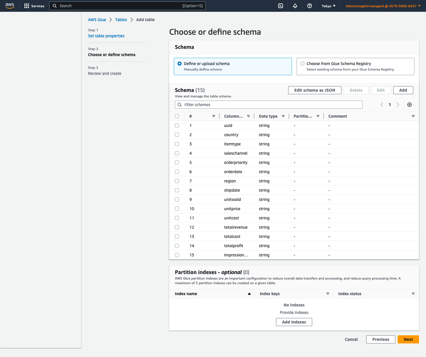
-
- Choose Next, then choose Create.
Create an AWS Glue streaming ETL job
Next, you create an AWS Glue streaming job. AWS Glue 3.0 and later supports Apache Hudi natively, so we use this native integration to ingest into a Hudi table. Complete the following steps to create the AWS Glue streaming job:
- On the AWS Glue Studio console, choose Spark script editor and choose Create.
- Under Job details tab, for Name, enter a name for your job.
- For IAM Role, choose the IAM role for your AWS Glue job.
- For Type, select Spark Streaming.
- For Glue version, choose Glue 4.0 – Supports spark 3.3, Scala 2, Python 3.
- For Requested number of workers, enter
3. - Under Advanced properties, for Job parameters, choose Add new parameter.
- For Key, enter
--conf. - For Value, enter
spark.serializer=org.apache.spark.serializer.KryoSerializer --conf spark.sql.hive.convertMetastoreParquet=false. - Choose Add new parameter.
- For Key, enter
--datalake-formats. - For Value, enter
hudi. - For Script path, enter
s3://<S3BucketName>/scripts/. - For Temporary path, enter
s3://<S3BucketName>/temporary/. - Optionally, for Spark UI logs path, enter
s3://<S3BucketName>/sparkHistoryLogs/.

- On the Script tab, enter the following script into the AWS Glue Studio editor and choose Create.
The near-real-time streaming job enriches data by joining a Kinesis data stream with a DynamoDB table that contains frequently updated reference data. The enriched dataset is loaded into the target Hudi table in the data lake. Replace <S3BucketName> with your bucket that you created via AWS CloudFormation:
- Choose Run to start the streaming job.
The following screenshot shows examples of the DataFrames data\_frame, country\_lookup\_df, and final\_frame.
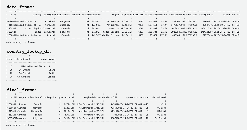
The AWS Glue job successfully joined records coming from the Kinesis data stream and the reference table in DynamoDB, and then ingested the joined records into Amazon S3 in Hudi format.
Create and run a Python script to generate sample data and load it into the Kinesis data stream
In this section, you create and run a Python to generate sample data and load it into the source Kinesis data stream. Complete the following steps:
- Log in to AWS Cloud9, your EC2 instance, or any other computing host that puts records in your data stream.
- Create a Python file called
generate-data-for-kds.py:
- Open the Python file and enter the following script:
This script puts a Kinesis data stream record every 2 seconds.
Simulate updating the reference table in the Aurora MySQL cluster
Now all the resources and configurations are ready. For this example, we want to add a 3-digit country code to the reference table. Let’s update records in the Aurora MySQL table to simulate changes. Complete the following steps:
- Make sure that the AWS Glue streaming job is already running.
- Connect to the primary DB instance again, as described earlier.
- Enter your SQL commands to update records:
Now the reference table in the Aurora MySQL source database has been updated. Then the changes are automatically replicated to the reference table in DynamoDB.

The following tables show records in data\_frame, country\_lookup\_df, and final\_frame. In country\_lookup\_df and final\_frame, the combinedname column has values formatted as <2-digit-country-code>-<3-digit-country-code>-<country-name>, which shows that the changed records in the referenced table are reflected in the table without restarting the AWS Glue streaming job. It means that the AWS Glue job successfully joins the incoming records from the Kinesis data stream with the reference table even when the reference table is changing.
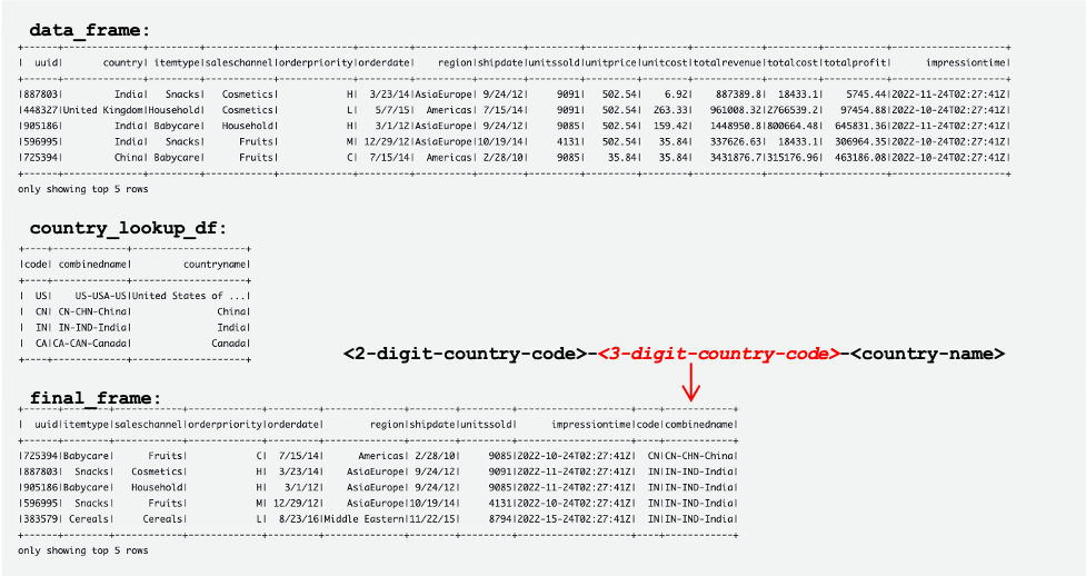
Query the Hudi table using Athena
Let’s query the Hudi table using Athena to see the records in the destination table. Complete the following steps:
- Make sure that the script and the AWS Glue Streaming job is still working:
- The Python script (
generate-data-for-kds.py) is still running. - The generated data is being sent to the data stream.
- The AWS Glue streaming job is still running.
- The Python script (
- On the Athena console, run the following SQL in the query editor:
The following query result shows the records that are processed before the referenced table was changed. Records in the combinedname column are similar to <2-digit-country-code>-<country-name>.

The following query result shows the records that are processed after the referenced table was changed. Records in the combinedname column are similar to <2-digit-country-code>-<3-digit-country-code>-<country-name>.

Now you understand that the changed reference data is successfully reflected in the target Hudi table joining records from the Kinesis data stream and the reference data in DynamoDB.
Clean up
As the final step, clean up the resources:
- Delete the Kinesis data stream.
- Delete the AWS DMS migration task, endpoint, and replication instance.
- Stop and delete the AWS Glue streaming job.
- Delete the AWS Cloud9 environment.
- Delete the CloudFormation template.
Conclusion
Building and maintaining a transactional data lake that involves real-time data ingestion and processing has multiple variable components and decisions to be made, such as what ingestion service to use, how to store your reference data, and what transactional data lake framework to use. In this post, we provided the implementation details of such a pipeline, using AWS native components as the building blocks and Apache Hudi as the open-source framework for a transactional data lake.
We believe that this solution can be a starting point for organizations looking to implement a new data lake with such requirements. Additionally, the different components are fully pluggable and can be mixed and matched to existing data lakes to target new requirements or migrate existing ones, addressing their pain points.
About the authors
 Manish Kola is a Data Lab Solutions Architect at AWS, where he works closely with customers across various industries to architect cloud-native solutions for their data analytics and AI needs. He partners with customers on their AWS journey to solve their business problems and build scalable prototypes. Before joining AWS, Manish’s experience includes helping customers implement data warehouse, BI, data integration, and data lake projects.
 Santosh Kotagiri is a Solutions Architect at AWS with experience in data analytics and cloud solutions leading to tangible business results. His expertise lies in designing and implementing scalable data analytics solutions for clients across industries, with a focus on cloud-native and open-source services. He is passionate about leveraging technology to drive business growth and solve complex problems.
 Chiho Sugimoto is a Cloud Support Engineer on the AWS Big Data Support team. She is passionate about helping customers build data lakes using ETL workloads. She loves planetary science and enjoys studying the asteroid Ryugu on weekends.
 Noritaka Sekiyama is a Principal Big Data Architect on the AWS Glue team. He is responsible for building software artifacts to help customers. In his spare time, he enjoys cycling with his new road bike.
Data transformation plays a pivotal role in providing the necessary data insights for businesses in any organization, small and large. To gain these insights, customers often perform ETL (extract, transform, and load) jobs from their source systems and output an enriched dataset. Many organizations today are using AWS Glue to build ETL pipelines that bring data from disparate sources and store the data in repositories like a data lake, database, or data warehouse for further consumption. These organizations are looking for ways they can reduce cost across their IT environments and still be operationally performant and efficient.
Picture a scenario where you, the VP of Data and Analytics, are in charge of your data and analytics environments and workloads running on AWS where you manage a team of data engineers and analysts. This team is allowed to create AWS Glue for Spark jobs in development, test, and production environments. During testing, one of the jobs wasn’t configured to automatically scale its compute resources, resulting in jobs timing out, costing the organization more than anticipated. The next steps usually include completing an analysis of the jobs, looking at cost reports to see which account generated the spike in usage, going through logs to see when what happened with the job, and so on. After the ETL job has been corrected, you may want to implement monitoring and set standard alert thresholds for your AWS Glue environment.
This post will help organizations proactively monitor and cost optimize their AWS Glue environments by providing an easier path for teams to measure efficiency of their ETL jobs and align configuration details according to organizational requirements. Included is a solution you will be able to deploy that will notify your team via email about any Glue job that has been configured incorrectly. Additionally, a weekly report is generated and sent via email that aggregates resource usage and provides cost estimates per job.
AWS Glue cost considerations
AWS Glue for Apache Spark jobs are provisioned with a number of workers and a worker type. These jobs can be either G.1X, G.2X, G.4X, G.8X or Z.2X (Ray) worker types that map to data processing units (DPUs). DPUs include a certain amount of CPU, memory, and disk space. The following table contains more details.
| Worker Type | DPUs | vCPUs | Memory (GB) | Disk (GB) |
| G.1X | 1 | 4 | 16 | 64 |
| G.2X | 2 | 8 | 32 | 128 |
| G.4X | 4 | 16 | 64 | 256 |
| G.8X | 8 | 32 | 128 | 512 |
| Z.2X | 2 | 8 | 32 | 128 |
For example, if a job is provisioned with 10 workers as G.1X worker type, the job will have access to 40 vCPU and 160 GB of RAM to process data and double using G.2X. Over-provisioning workers can lead to increased cost, due to not all workers being utilized efficiently.
In April 2022, Auto Scaling for AWS Glue was released for AWS Glue version 3.0 and later, which includes AWS Glue for Apache Spark and streaming jobs. Enabling auto scaling on your Glue for Apache Spark jobs will allow you to only allocate workers as needed, up to the worker maximum you specify. We recommend enabling auto scaling for your AWS Glue 3.0 & 4.0 jobs because this feature will help reduce cost and optimize your ETL jobs.
Amazon CloudWatch metrics are also a great way to monitor your AWS Glue environment by creating alarms for certain metrics like average CPU or memory usage. To learn more about how to use CloudWatch metrics with AWS Glue, refer to Monitoring AWS Glue using Amazon CloudWatch metrics.
The following solution provides a simple way to set AWS Glue worker and job duration thresholds, configure monitoring, and receive emails for notifications on how your AWS Glue environment is performing. If a Glue job finishes and detects worker or job duration thresholds were exceeded, it will notify you after the job run has completed, failed, or timed out.
Solution overview
The following diagram illustrates the solution architecture.

When you deploy this application via AWS Serverless Application Model (AWS SAM), it will ask what AWS Glue worker and job duration thresholds you would like to set to monitor the AWS Glue for Apache Spark and AWS Glue for Ray jobs running in that account. The solution will use these values as the decision criteria when invoked. The following is a breakdown of each step in the architecture:
- Any AWS Glue for Apache Spark job that succeeds, fails, stops, or times out is sent to Amazon EventBridge.
- EventBridge picks up the event from AWS Glue and triggers an AWS Lambda function.
- The Lambda function processes the event and determines if the data and analytics team should be notified about the particular job run. The function performs the following tasks:
- The function sends an email using Amazon Simple Notification Service (Amazon SNS) if needed.
- If the AWS Glue job succeeded or was stopped without going over the worker or job duration thresholds, or is tagged to not be monitored, no alerts or notifications are sent.
- If the job succeeded but ran with a worker or job duration thresholds higher than allowed, or the job either failed or timed out, Amazon SNS sends a notification to the designated email with information about the AWS Glue job, run ID, and reason for alerting, along with a link to the specific run ID on the AWS Glue console.
- The function logs the job run information to Amazon DynamoDB for a weekly aggregated report delivered to email. The Dynamo table has Time to Live enabled for 7 days, which keeps the storage to minimum.
- The function sends an email using Amazon Simple Notification Service (Amazon SNS) if needed.
- Once a week, the data within DynamoDB is aggregated by a separate Lambda function with meaningful information like longest-running jobs, number of retries, failures, timeouts, cost analysis, and more.
- Amazon Simple Email Service (Amazon SES) is used to deliver the report because it can be better formatted than using Amazon SNS. The email is formatted via HTML output that provides tables for the aggregated job run data.
- The data and analytics team is notified about the ongoing job runs through Amazon SNS, and they receive the weekly aggregation report through Amazon SES.
Note that AWS Glue Python shell and streaming ETL jobs are not supported because they’re not in scope of this solution.
Prerequisites
You must have the following prerequisites:
- An AWS account to deploy the solution to
- Proper AWS Identity and Access Management (IAM) privileges to create the resources
- The AWS SAM CLI to build and deploy the solution button below, to run template on your AWS environment
Deploy the solution
This AWS SAM application provisions the following resources:
- Two EventBridge rules
- Two Lambda functions
- An SNS topic and subscription
- A DynamoDB table
- An SES subscription
- The required IAM roles and policies
To deploy the AWS SAM application, complete the following steps:
Clone the aws-samples GitHub repository:
git clone https://github.com/aws-samples/aws-glue-job-tracker.gitDeploy the AWS SAM application:
cd aws-glue-job-trackersam deploy --guided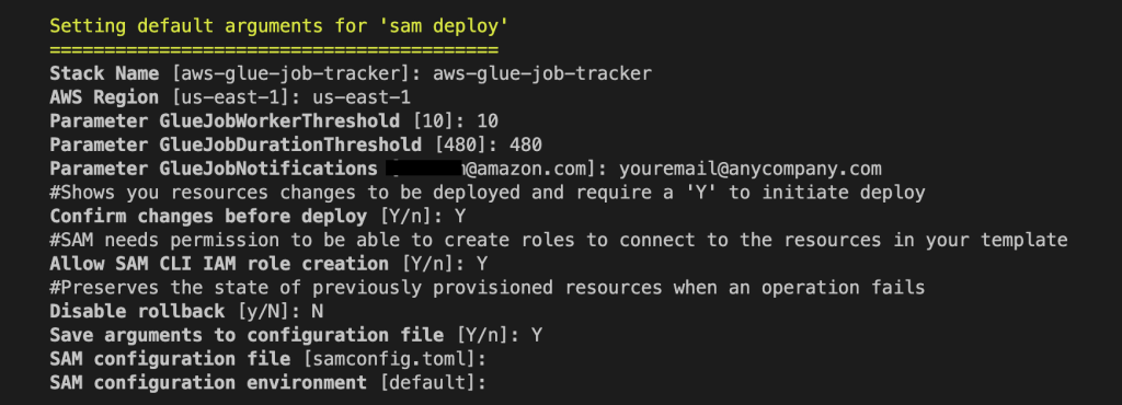
Provide the following parameters:
- GlueJobWorkerThreshold – Enter the maximum number of workers you want an AWS Glue job to be able to run with before sending threshold alert. The default is 10. An alert will be sent if a Glue job runs with higher workers than specified.
- GlueJobDurationThreshold – Enter the maximum duration in minutes you want an AWS Glue job to run before sending threshold alert. The default is 480 minutes (8 hours). An alert will be sent if a Glue job runs with higher job duration than specified.
- GlueJobNotifications – Enter an email or distribution list of those who need to be notified through Amazon SNS and Amazon SES. You can go to the SNS topic after the deployment is complete and add emails as needed.
To receive emails from Amazon SNS and Amazon SES, you must confirm your subscriptions. After the stack is deployed, check your email that was specified in the template and confirm by choosing the link in each message. When the application is successfully provisioned, it will begin monitoring your AWS Glue for Apache Spark job environment. The next time a job fails, times out, or exceeds a specified threshold, you will receive an email via Amazon SNS. For example, the following screenshot shows an SNS message about a job that succeeded but had a job duration threshold violation.

You might have jobs that need to run at a higher worker or job duration threshold, and you don’t want the solution to evaluate them. You can simply tag that job with the key/value of remediate and false. The step function will still be invoked, but will use the PASS state when it recognizes the tag. For more information on job tagging, refer to AWS tags in AWS Glue.

Configure weekly reporting
As mentioned previously, when an AWS Glue for Apache Spark job succeeds, fails, times out, or is stopped, EventBridge forwards this event to Lambda, where it logs specific information about each job run. Once a week, a separate Lambda function queries DynamoDB and aggregates your job runs to provide meaningful insights and recommendations about your AWS Glue for Apache Spark environment. This report is sent via email with a tabular structure as shown in the following screenshot. It’s meant for top-level visibility so you’re able to see your longest job runs over time, jobs that have had many retries, failures, and more. It also provides an overall cost calculation as an estimate of what each AWS Glue job will cost for that week. It should not be used as a guaranteed cost. If you would like to see exact cost per job, the AWS Cost and Usage Report is the best resource to use. The following screenshot shows one table (of five total) from the AWS Glue report function.
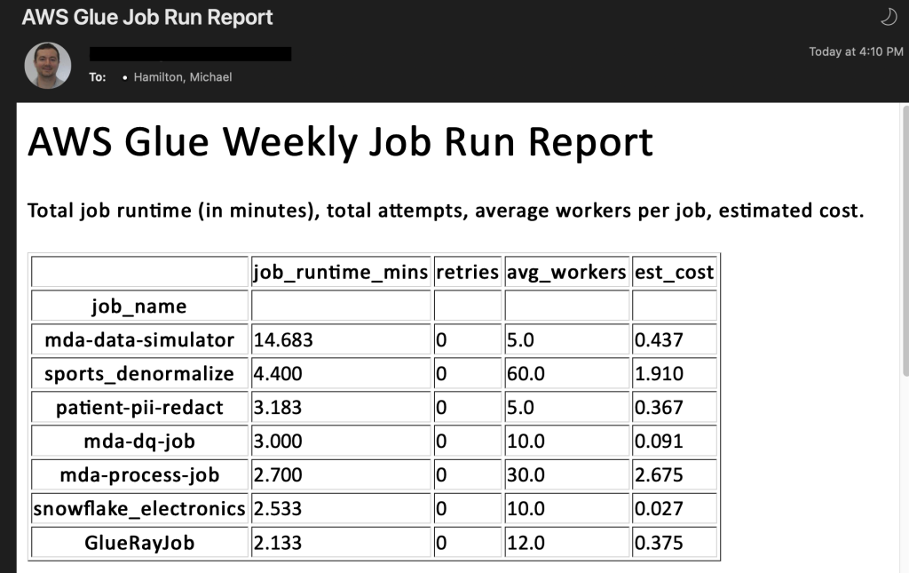
Clean up
If you don’t want to run the solution anymore, delete the AWS SAM application for each account that it was provisioned in. To delete your AWS SAM stack, run the following command from your project directory:
sam deleteConclusion
In this post, we discussed how you can monitor and cost-optimize your AWS Glue job configurations to comply with organizational standards and policy. This method can provide cost controls over AWS Glue jobs across your organization. Some other ways to help control the costs of your AWS Glue for Apache Spark jobs include the newly released AWS Glue Flex jobs and Auto Scaling. We also provided an AWS SAM application as a solution to deploy into your accounts. We encourage you to review the resources provided in this post to continue learning about AWS Glue. To learn more about monitoring and optimizing for cost using AWS Glue, please visit this recent blog. It goes in depth on all of the cost optimization options and includes a template that builds a CloudWatch dashboard for you with metrics about all of your Glue job runs.
About the authors
 Michael Hamilton is a Sr Analytics Solutions Architect focusing on helping enterprise customers in the south east modernize and simplify their analytics workloads on AWS. He enjoys mountain biking and spending time with his wife and three children when not working.
 Angus Ferguson is a Solutions Architect at AWS who is passionate about meeting customers across the world, helping them solve their technical challenges. Angus specializes in Data & Analytics with a focus on customers in the financial services industry.
This is a guest post by Cynthia Valeriano, Jaime Olivares, and Guillermo Puelles from DeFontana.
 |  |
Defontana develops fully cloud-based business applications for the administration and management of companies. Based in Santiago, Chile, with operations in Peru, Mexico, and most recently Colombia, our main product is a 100% cloud-based enterprise resource planning (ERP) system that has been providing value to our business customers for about 20 years. In addition to our core ERP product, we have developed integration modules for ecommerce, banks, financial and regulatory institutions, digital signatures, business reports, and many other solutions. Our goal is to continue building solutions for customers and make Defontana the best business administration tool in Chile and Latin America.
Most of our customers are small and medium businesses (SMBs) who need to optimize their resources. Our ERP system helps customers manage cash flow, time, human resources (HR), and other resources. As we were exploring how to continue innovating for our customers and looking for an embedded analytics solution, we chose Amazon QuickSight, which allows us to seamlessly integrate data-driven experiences into our web application.
In this post, we discuss how QuickSight has sped up our development time, enabled us to provide more value to our customers, and even improved our own internal operations.
Saving development time by embedding QuickSight
We built our ERP service as a web application from the beginning. 10 years ago, this was a big differentiator for us, but to continue to serve the SMBs that trust us for information on a daily basis, we wanted to offer even more advanced analytics. By embedding QuickSight into our web application, we have been able to provide business intelligence (BI) functionalities to customers two or three times faster than we would have if we had opted for libraries for generating HTML reports. Thanks to our embedded QuickSight solution, we are able to focus more of our energy on analyzing the requirements and functionalities that we want to offer our customers in each BI report.
The following screenshots show our ERP service, accessed on a web browser, with insights and rich visualizations by QuickSight.
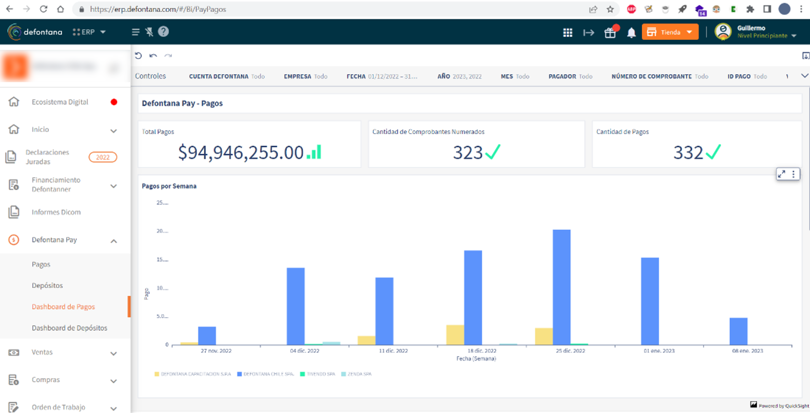
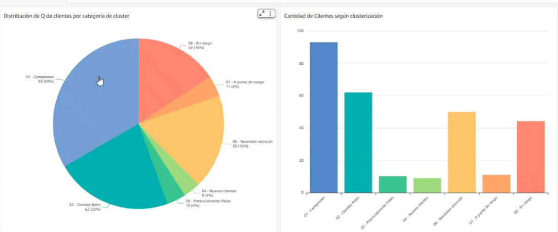
We enjoy using QuickSight because of how well it integrates with other AWS services. Our data is stored in a legacy relational database management system (RDMS), Amazon Aurora, and Amazon DynamoDB. We are in the process of moving away from that legacy RDMS to PostgreSQL through a Babelfish for Aurora PostgreSQL project. This will allow us to reduce costs while also being able to use a multi-Region database with disaster recovery in the future. This would have been too expensive with the legacy RDMS. To seamlessly transfer data from these databases to Amazon Simple Storage Service (Amazon S3), we use AWS Database Migration Service (AWS DMS). Then, AWS Glue allows us to generate several extract, transform, and load (ETL) processes to prepare the data in Amazon S3 to be used in QuickSight. Finally, we use Amazon Athena to generate views to be used as base information in QuickSight.
Providing essential insights for SMB customers
QuickSight simplifies the generation of dashboards. We have made several out-of-the-box dashboards in QuickSight for our customers that they can use directly on our web app right after they sign up. These dashboards provide insights on sales, accounting, cash flow, financial information, and customer clusters based on their data in our ERP service. These free-to-use reports can be used by all customers in the system. We also have dashboards that can be activated by any user of the system for a trial period. Since we launched add-on dashboards, more than 300 companies have activated it, with over 100 of them choosing to continue using it after the free trial.
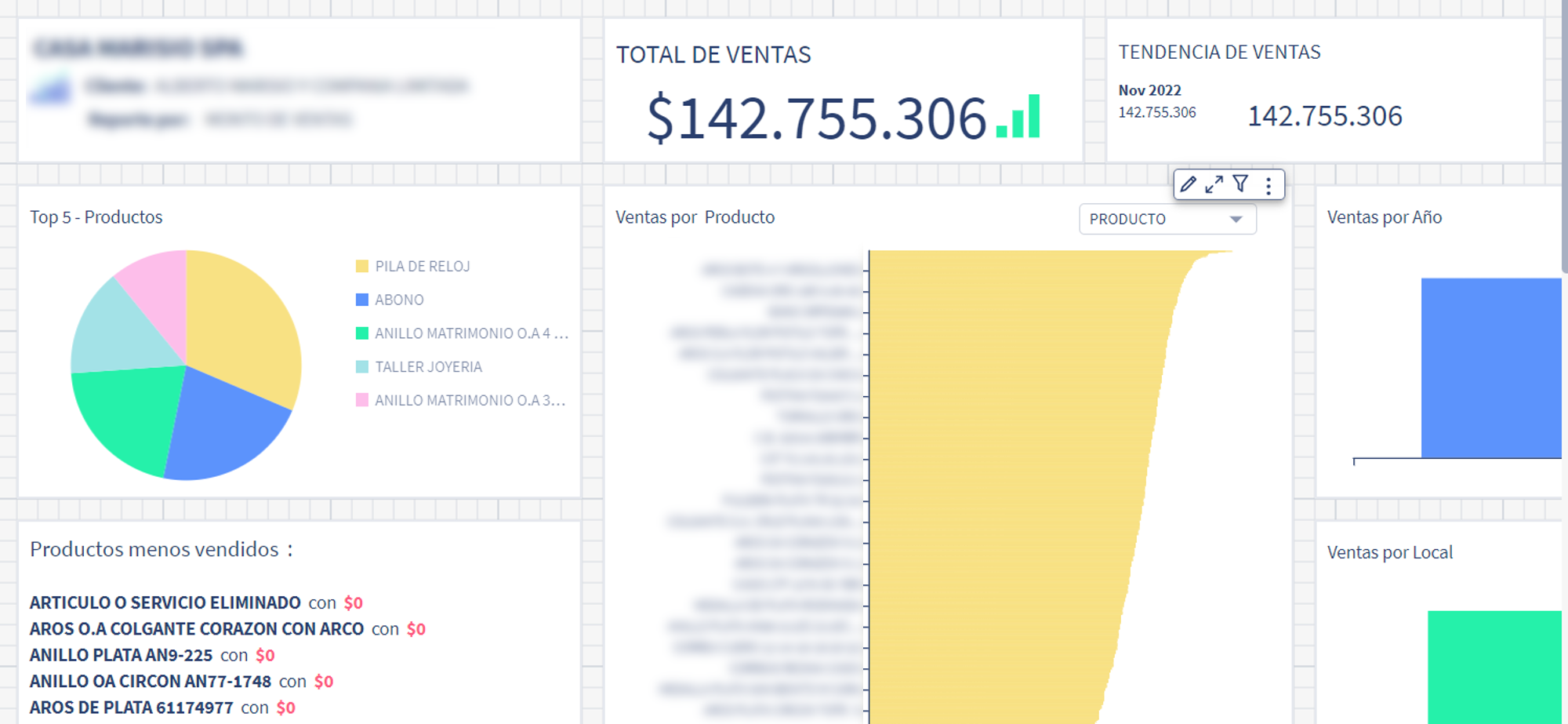
Besides generic reports, we have created several tailor-made dashboards according to the specific requirements of each customer. These are managed through a customer-focused development process by our engineering team according to the specifications of each customer. With this option, our customers can get reports on accounts payable, accounts receivable, supply information (purchase order flow, receipts and invoices sent by suppliers), inventory details, and more. We have more than 50 customers who have worked with us on tailor-made dashboards. With the broad range of functionalities within QuickSight, we can offer many data visualization options to our customers.
Empowering our own operations
Beyond using QuickSight to serve our customers, we also use QuickSight for our own BI reporting. So far, we have generated more than 80 dashboards to analyze different business flows. For example, we monitor daily sales in specific services, accounting, software as a service (SaaS) metrics, and the operation of our customers. We do all of this from within our own web application, with the power of QuickSight, giving us the opportunity to experience the interface just like our customers do. In 2023, one of our top goals is to provide a 360-degree view of Defontana using QuickSight.
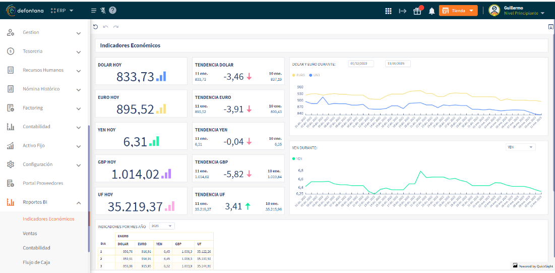
Conclusion
QuickSight has enabled us to seamlessly embed analytics into our ERP service, providing valuable insights to our SMB customers. We have been able to cut costs and continue to grow throughout Latin America. We plan to use QuickSight even more within our own organization, making us more data-driven. QuickSight will empower us to democratize the information that our own employees receive, establish better processes, and create more tools to analyze customer information for behavioral patterns, which we can use to better meet our customers’ needs.
To learn more about how you can embed customized data visuals and interactive dashboards into any application, visit Amazon QuickSight Embedded.
About the authors
 Cynthia Valeriano is a Business Intelligence Developer of at Defontana, with skills focused on data analysis and visualization. With 3 years of experience in administrative areas and 2 years of experience in business intelligence projects, she has been in charge of implementing data migration and transformation tasks with various AWS tools, such as AWS DMS and AWS Glue, in addition to generating multiple dashboards in Amazon QuickSight.
 Jaime Olivares is a Senior software developer at Defontana, with 6 years of experience in the development of various technologies focused on the analysis of solutions and customer requirements. Experience with AWS in various services, including product development through QuickSight for the analysis of business and accounting data.
 Guillermo Puelles is a Technical Manager of the “Appia” Integrations team at Defontana, with 9 years of experience in software development and 5 years working with AWS tools. Responsible for planning and managing various projects for the implementation of BI solutions through QuickSight and other AWS services.
Apache Iceberg is an open table format for large datasets in Amazon Simple Storage Service (Amazon S3) and provides fast query performance over large tables, atomic commits, concurrent writes, and SQL-compatible table evolution. When you build your transactional data lake using Apache Iceberg to solve your functional use cases, you need to focus on operational use cases for your S3 data lake to optimize the production environment. Some of the important non-functional use cases for an S3 data lake that organizations are focusing on include storage cost optimizations, capabilities for disaster recovery and business continuity, cross-account and multi-Region access to the data lake, and handling increased Amazon S3 request rates.
In this post, we show you how to improve operational efficiencies of your Apache Iceberg tables built on Amazon S3 data lake and Amazon EMR big data platform.
Optimize data lake storage
One of the major advantages of building modern data lakes on Amazon S3 is it offers lower cost without compromising on performance. You can use Amazon S3 Lifecycle configurations and Amazon S3 object tagging with Apache Iceberg tables to optimize the cost of your overall data lake storage. An Amazon S3 Lifecycle configuration is a set of rules that define actions that Amazon S3 applies to a group of objects. There are two types of actions:
- Transition actions – These actions define when objects transition to another storage class; for example, Amazon S3 Standard to Amazon S3 Glacier.
- Expiration actions – These actions define when objects expire. Amazon S3 deletes expired objects on your behalf.
Amazon S3 uses object tagging to categorize storage where each tag is a key-value pair. From an Apache Iceberg perspective, it supports custom Amazon S3 object tags that can be added to S3 objects while writing and deleting into the table. Iceberg also let you configure a tag-based object lifecycle policy at the bucket level to transition objects to different Amazon S3 tiers. With the s3.delete.tags config property in Iceberg, objects are tagged with the configured key-value pairs before deletion. When the catalog property s3.delete-enabled is set to false, the objects are not hard-deleted from Amazon S3. This is expected to be used in combination with Amazon S3 delete tagging, so objects are tagged and removed using an Amazon S3 lifecycle policy. This property is set to true by default.
The example notebook in this post shows an example implementation of S3 object tagging and lifecycle rules for Apache Iceberg tables to optimize storage cost.
Implement business continuity
Amazon S3 gives any developer access to the same highly scalable, reliable, fast, inexpensive data storage infrastructure that Amazon uses to run its own global network of web sites. Amazon S3 is designed for 99.999999999% (11 9’s) of durability, S3 Standard is designed for 99.99% availability, and Standard – IA is designed for 99.9% availability. Still, to make your data lake workloads highly available in an unlikely outage situation, you can replicate your S3 data to another AWS Region as a backup. With S3 data residing in multiple Regions, you can use an S3 multi-Region access point as a solution to access the data from the backup Region. With Amazon S3 multi-Region access point failover controls, you can route all S3 data request traffic through a single global endpoint and directly control the shift of S3 data request traffic between Regions at any time. During a planned or unplanned regional traffic disruption, failover controls let you control failover between buckets in different Regions and accounts within minutes. Apache Iceberg supports access points to perform S3 operations by specifying a mapping of bucket to access points. We include an example implementation of an S3 access point with Apache Iceberg later in this post.
Increase Amazon S3 performance and throughput
Amazon S3 supports a request rate of 3,500 PUT/COPY/POST/DELETE or 5,500 GET/HEAD requests per second per prefix in a bucket. The resources for this request rate aren’t automatically assigned when a prefix is created. Instead, as the request rate for a prefix increases gradually, Amazon S3 automatically scales to handle the increased request rate. For certain workloads that need a sudden increase in the request rate for objects in a prefix, Amazon S3 might return 503 Slow Down errors, also known as S3 throttling. It does this while it scales in the background to handle the increased request rate. Also, if supported request rates are exceeded, it’s a best practice to distribute objects and requests across multiple prefixes. Implementing this solution to distribute objects and requests across multiple prefixes involves changes to your data ingress or data egress applications. Using Apache Iceberg file format for your S3 data lake can significantly reduce the engineering effort through enabling the ObjectStoreLocationProvider feature, which adds an S3 hash [0*7FFFFF] prefix in your specified S3 object path.
Iceberg by default uses the Hive storage layout, but you can switch it to use the ObjectStoreLocationProvider. This option is not enabled by default to provide flexibility to choose the location where you want to add the hash prefix. With ObjectStoreLocationProvider, a deterministic hash is generated for each stored file and a subfolder is appended right after the S3 folder specified using the parameter write.data.path (write.object-storage-path for Iceberg version 0.12 and below). This ensures that files written to Amazon S3 are equally distributed across multiple prefixes in your S3 bucket, thereby minimizing the throttling errors. In the following example, we set the write.data.path value as s3://my-table-data-bucket, and Iceberg-generated S3 hash prefixes will be appended after this location:
Your S3 files will be arranged under MURMUR3 S3 hash prefixes like the following:
Using Iceberg ObjectStoreLocationProvider is not a foolproof mechanism to avoid S3 503 errors. You still need to set appropriate EMRFS retries to provide additional resiliency. You can adjust your retry strategy by increasing the maximum retry limit for the default exponential backoff retry strategy or enabling and configuring the additive-increase/multiplicative-decrease (AIMD) retry strategy. AIMD is supported for Amazon EMR releases 6.4.0 and later. For more information, refer to Retry Amazon S3 requests with EMRFS.
In the following sections, we provide examples for these use cases.
Storage cost optimizations
In this example, we use Iceberg’s S3 tags feature with the write tag as write-tag-name=created and delete tag as delete-tag-name=deleted. This example is demonstrated on an EMR version emr-6.10.0 cluster with installed applications Hadoop 3.3.3, Jupyter Enterprise Gateway 2.6.0, and Spark 3.3.1. The examples are run on a Jupyter Notebook environment attached to the EMR cluster. To learn more about how to create an EMR cluster with Iceberg and use Amazon EMR Studio, refer to Use an Iceberg cluster with Spark and the Amazon EMR Studio Management Guide, respectively.
The following examples are also available in the sample notebook in the aws-samples GitHub repo for quick experimentation.
Configure Iceberg on a Spark session
Configure your Spark session using the %%configure magic command. You can use either the AWS Glue Data Catalog (recommended) or a Hive catalog for Iceberg tables. In this example, we use a Hive catalog, but we can change to the Data Catalog with the following configuration:
Before you run this step, create a S3 bucket and an iceberg folder in your AWS account with the naming convention <your-iceberg-storage-blog>/iceberg/.
Update your-iceberg-storage-blog in the following configuration with the bucket that you created to test this example. Note the configuration parameters s3.write.tags.write-tag-name and s3.delete.tags.delete-tag-name, which will tag the new S3 objects and deleted objects with corresponding tag values. We use these tags in later steps to implement S3 lifecycle policies to transition the objects to a lower-cost storage tier or expire them based on the use case.
Create an Apache Iceberg table using Spark-SQL
Now we create an Iceberg table for the Amazon Product Reviews Dataset:
In the next step, we load the table with the dataset using Spark actions.
Load data into the Iceberg table
While inserting the data, we partition the data by review\_date as per the table definition. Run the following Spark commands in your PySpark notebook:
Insert a single record into the same Iceberg table so that it creates a partition with the current review\_date:
You can check the new snapshot is created after this append operation by querying the Iceberg snapshot:
You will see an output similar to the following showing the operations performed on the table.

Check the S3 tag population
You can use the AWS Command Line Interface (AWS CLI) or the AWS Management Console to check the tags populated for the new writes. Let’s check the tag corresponding to the object created by a single row insert.
On the Amazon S3 console, check the S3 folder s3://your-iceberg-storage-blog/iceberg/db/amazon\_reviews\_iceberg/data/ and point to the partition review\_date\_year=2023/. Then check the Parquet file under this folder to check the tags associated with the data file in Parquet format.
From the AWS CLI, run the following command to see that the tag is created based on the Spark configuration spark.sql.catalog.dev.s3.write.tags.write-tag-name":"created":
In this step, we delete a record from the Iceberg table and expire the snapshot corresponding to the deleted record. We delete the new single record that we inserted with the current review\_date:
We can now check that a new snapshot was created with the operation flagged as delete:

This is useful if we want to time travel and check the deleted row in the future. In that case, we have to query the table with the snapshot-id corresponding to the deleted row. However, we don’t discuss time travel as part of this post.
We expire the old snapshots from the table and keep only the last two. You can modify the query based on your specific requirements to retain the snapshots:
If we run the same query on the snapshots, we can see that we have only two snapshots available:

From the AWS CLI, you can run the following command to see that the tag is created based on the Spark configuration spark.sql.catalog.dev.s3. delete.tags.delete-tag-name":"deleted":
The snapshots that have expired show the latest snapshot ID as null.

Create S3 lifecycle rules to transition the buckets to a different storage tier
Create a lifecycle configuration for the bucket to transition objects with the delete-tag-name=deleted S3 tag to the Glacier Instant Retrieval class. Amazon S3 runs lifecycle rules one time every day at midnight Universal Coordinated Time (UTC), and new lifecycle rules can take up to 48 hours to complete the first run. Amazon S3 Glacier is well suited to archive data that needs immediate access (with milliseconds retrieval). With S3 Glacier Instant Retrieval, you can save up to 68% on storage costs compared to using the S3 Standard-Infrequent Access (S3 Standard-IA) storage class, when the data is accessed once per quarter.

When you want to access the data back, you can bulk restore the archived objects. After you restore the objects back in S3 Standard class, you can register the metadata and data as an archival table for query purposes. The metadata file location can be fetched from the metadata log entries metatable as illustrated earlier. As mentioned before, the latest snapshot ID with Null values indicates expired snapshots. We can take one of the expired snapshots and do the bulk restore:
Capabilities for disaster recovery and business continuity, cross-account and multi-Region access to the data lake
Because Iceberg doesn’t support relative paths, you can use access points to perform Amazon S3 operations by specifying a mapping of buckets to access points. This is useful for multi-Region access, cross-Region access, disaster recovery, and more.
For cross-Region access points, we need to additionally set the use-arn-region-enabled catalog property to true to enable S3FileIO to make cross-Region calls. If an Amazon S3 resource ARN is passed in as the target of an Amazon S3 operation that has a different Region than the one the client was configured with, this flag must be set to ‘true‘ to permit the client to make a cross-Region call to the Region specified in the ARN, otherwise an exception will be thrown. However, for the same or multi-Region access points, the use-arn-region-enabled flag should be set to ‘false’.
For example, to use an S3 access point with multi-Region access in Spark 3.3, you can start the Spark SQL shell with the following code:
In this example, the objects in Amazon S3 on my-bucket1 and my-bucket2 buckets use the arn:aws:s3::123456789012:accesspoint:mfzwi23gnjvgw.mrap access point for all Amazon S3 operations.
For more details on using access points, refer to Using access points with compatible Amazon S3 operations.
Let’s say your table path is under mybucket1, so both mybucket1 in Region 1 and mybucket2 in Region have paths of mybucket1 inside the metadata files. At the time of the S3 (GET/PUT) call, we replace the mybucket1 reference with a multi-Region access point.
Handling increased S3 request rates
When using ObjectStoreLocationProvider (for more details, see Object Store File Layout), a deterministic hash is generated for each stored file, with the hash appended directly after the write.data.path. The problem with this is that the default hashing algorithm generates hash values up to Integer MAX\_VALUE, which in Java is (2^31)-1. When this is converted to hex, it produces 0x7FFFFFFF, so the first character variance is restricted to only [0-8]. As per Amazon S3 recommendations, we should have the maximum variance here to mitigate this.
Starting from Amazon EMR 6.10, Amazon EMR added an optimized location provider that makes sure the generated prefix hash has uniform distribution in the first two characters using the character set from [0-9][A-Z][a-z].
This location provider has been recently open sourced by Amazon EMR via Core: Improve bit density in object storage layout and should be available starting from Iceberg 1.3.0.
To use, make sure the iceberg.enabled classification is set to true, and write.location-provider.impl is set to org.apache.iceberg.emr.OptimizedS3LocationProvider.
The following is a sample Spark shell command:
The following example shows that when you enable the object storage in your Iceberg table, it adds the hash prefix in your S3 path directly after the location you provide in your DDL.
Define the table write.object-storage.enabled parameter and provide the S3 path, after which you want to add the hash prefix using write.data.path (for Iceberg Version 0.13 and above) or write.object-storage.path (for Iceberg Version 0.12 and below) parameters.

Insert data into the table you created.

The hash prefix is added right after the /current/ prefix in the S3 path as defined in the DDL.

Clean up
After you complete the test, clean up your resources to avoid any recurring costs:
- Delete the S3 buckets that you created for this test.
- Delete the EMR cluster.
- Stop and delete the EMR notebook instance.
Conclusion
As companies continue to build newer transactional data lake use cases using Apache Iceberg open table format on very large datasets on S3 data lakes, there will be an increased focus on optimizing those petabyte-scale production environments to reduce cost, improve efficiency, and implement high availability. This post demonstrated mechanisms to implement the operational efficiencies for Apache Iceberg open table formats running on AWS.
To learn more about Apache Iceberg and implement this open table format for your transactional data lake use cases, refer to the following resources:
- Apache Iceberg table specifications
- Apache Iceberg support on Amazon EMR
- Use a cluster with Iceberg installed
About the Authors
 Avijit Goswami is a Principal Solutions Architect at AWS specialized in data and analytics. He supports AWS strategic customers in building high-performing, secure, and scalable data lake solutions on AWS using AWS managed services and open-source solutions. Outside of his work, Avijit likes to travel, hike in the San Francisco Bay Area trails, watch sports, and listen to music.
 Rajarshi Sarkar is a Software Development Engineer at Amazon EMR/Athena. He works on cutting-edge features of Amazon EMR/Athena and is also involved in open-source projects such as Apache Iceberg and Trino. In his spare time, he likes to travel, watch movies, and hang out with friends.
 Prashant Singh is a Software Development Engineer at AWS. He is interested in Databases and Data Warehouse engines and has worked on Optimizing Apache Spark performance on EMR. He is an active contributor in open source projects like Apache Spark and Apache Iceberg. During his free time, he enjoys exploring new places, food and hiking.
Detecting anomalies in real time from high-throughput streams is key for informing on timely decisions in order to adapt and respond to unexpected scenarios. Stream processing frameworks such as Apache Flink empower users to design systems that can ingest and process continuous flows of data at scale. In this post, we present a streaming time series anomaly detection algorithm based on matrix profiles and left-discords, inspired by Lu et al., 2022, with Apache Flink, and provide a working example that will help you get started on a managed Apache Flink solution using Amazon Kinesis Data Analytics.
Challenges of anomaly detection
Anomaly detection plays a key role in a variety of real-world applications, such as fraud detection, sales analysis, cybersecurity, predictive maintenance, and fault detection, among others. The majority of these use cases require actions to be taken in near real-time. For instance, card payment networks must be able to identify and reject potentially fraudulent transactions before processing them. This raises the challenge to design near-real-time anomaly detection systems that are able to scale to ultra-fast arriving data streams.
Another key challenge that anomaly detection systems face is concept drift. The ever-changing nature of some use cases requires models to dynamically adapt to new scenarios. For instance, in a predictive maintenance scenario, you could use several Internet of Things (IoT) devices to monitor the vibrations produced by an electric motor with the objective of detecting anomalies and preventing unrecoverable damage. Sounds emitted by the vibrations of the motor can vary significantly over time due to different environmental conditions such as temperature variations, and this shift in pattern can invalidate the model. This class of scenarios creates the necessity for online learning—the ability of the model to continuously learn from new data.
Time series anomaly detection
Time series are a particular class of data that incorporates time in their structuring. The data points that characterize a time series are recorded in an orderly fashion and are chronological in nature. This class of data is present in every industry and is common at the core of many business requirements or key performance indicators (KPIs). Natural sources of time series data include credit card transactions, sales, sensor measurements, machine logs, and user analytics.
In the time series domain, an anomaly can be defined as a deviation from the expected patterns that characterize the time series. For instance, a time series can be characterized by its expected ranges, trends, seasonal, or cyclic patterns. Any significant alteration of this normal flow of data points is considered an anomaly.
Detecting anomalies can be more or less challenging depending on the domain. For instance, a threshold-based approach might be suitable for time series that are informed of their expected ranges, such as the working temperature of a machine or CPU utilization. On the other hand, applications such as fraud detection, cybersecurity, and predictive maintenance can’t be classified via simple rule-based approaches and require a more fine-grained mechanism to capture unexpected observations. Thanks to their parallelizable and event-driven setup, streaming engines such as Apache Flink provide an excellent environment for scaling real-time anomaly detection to fast-arriving data streams.
Solution overview
Apache Flink is a distributed processing engine for stateful computations over streams. A Flink program can be implemented in Java, Scala, or Python. It supports ingestion, manipulation, and delivery of data to the desired destinations. Kinesis Data Analytics allows you to run Flink applications in a fully managed environment on AWS.
Distance-based anomaly detection is a popular approach where a model is characterized by a number of internally stored data points that are used for comparison against the new incoming data points. At inference time, these methods compute distances and classify new data points according to how dissimilar they are from the past observations. In spite of the plethora of algorithms in literature, there is increasing evidence that distance-based anomaly detection algorithms are still competitive with the state of the art (Nakamura et al., 2020).
In this post, we present a streaming version of a distance-based unsupervised anomaly detection algorithm called time series discords, and explore some of the optimizations introduced by the Discord Aware Matrix Profile (DAMP) algorithm (Lu et al., 2022), which further develops the discords method to scale to trillions of data points.
Understanding the algorithm
A left-discord is a subsequence that is significantly dissimilar from all the subsequences that precede it. In this post, we demonstrate how to use the concept of left-discords to identify time series anomalies in streams using Kinesis Data Analytics for Apache Flink.
Let’s consider an unbounded stream and all its subsequences of length n. The m most recent subsequences will be stored and used for inference. When a new data point arrives, a new subsequence that includes the new event is formed. The algorithm compares this latest subsequence (query) to the m subsequences retained from the model, with the exclusion of the latest n subsequences because they overlap with the query and would therefore characterize a self-match. After computing these distances, the algorithm classifies the query as an anomaly if its distance from its closest non-self-matching subsequence is above a certain moving threshold.
For this post, we use a Kinesis data stream to ingest the input data, a Kinesis Data Analytics application to run the Flink anomaly detection program, and another Kinesis data stream to ingest the output produced by your application. For visualization purposes, we consume from the output stream using Kinesis Data Analytics Studio, which provides an Apache Zeppelin Notebook that we use to visualize and interact with the data in real time.
Implementation details
The Java application code for this example is available on GitHub. To download the application code, complete the following steps:
- Clone the remote repository using the following command:
- Navigate to the
amazon-kinesis-data-analytics-java-examples/AnomalyDetection/LeftDiscordsdirectory:
Let’s walk through the code step by step.
The MPStreamingJob class defines the data flow of the application, and the MPProcessFunction class defines the logic of the function that detects anomalies.
The implementation is best described by three core components:
- The Kinesis data stream source, used to read from the input stream
- The anomaly detection process function
- The Kinesis data stream sink, used to deliver the output into the output stream
The anomaly detection function is implemented as a ProcessFunction<String, String>. Its method MPProcessFunction#processElement is called for every data point:
For every incoming data point, the anomaly detection algorithm takes the following actions:
- Adds the record to the
timeSeriesData. - If it has observed at least
2 * sequenceLengthdata points, starts computing the matrix profile. - If it has observed at least
initializationPeriods * sequenceLengthdata points, starts outputting anomaly labels.
Following these actions, the MPProcessFunction function outputs an OutputWithLabel object with four attributes:
- index – The index of the data point in the time series
- input – The input data without any transformation (identity function)
- mp – The distance to the closest non-self-matching subsequence for the subsequence ending in index
- anomalyTag – A binary label that indicates whether the subsequence is an anomaly
In the provided implementation, the threshold is learned online by fitting a normal distribution to the matrix profile data:
In this example, the algorithm classifies as anomalies those subsequences whose distance from their nearest neighbor deviates significantly from the average minimum distance (more than two standard deviations away from the mean).
The TimeSeries class implements the data structure that retains the context window, namely, the internally stored records that are used for comparison against the new incoming records. In the provided implementation, the n most recent records are retained, and when the TimeSeries object is at capacity, the oldest records are overridden.
Prerequisites
Before you create a Kinesis Data Analytics application for this exercise, create two Kinesis data streams: InputStream and OutputStream in us-east-1. The Flink application will use these streams as its respective source and destination streams. To create these resources, launch the following AWS CloudFormation stack:
Alternatively, follow the instructions in Creating and Updating Data Streams.
Create the application
To create your application, complete the following steps:
- Clone the remote repository using the following command:
- Navigate to the
amazon-kinesis-data-analytics-java-examples/AnomalyDetection/LeftDiscords/coredirectory. - Create your JAR file by running the following Maven command in the core directory, which contains the
pom.xmlfile:
mvn package -Dflink.version=1.15.4 - Create an Amazon Simple Storage Service (Amazon S3) bucket and upload the file
target/left-discords-1.0.0.jar. - Create and run a Kinesis Data Analytics application as described in Create and Run the Kinesis Data Analytics Application:
- Use the
target/left-discords-1.0.0.jar. - Note that the input and output streams are called
InputStreamandOutputStream, respectively. - The provided example is set up to run in
us-east-1.
- Use the
Populate the input stream
You can populate InputStream by running the script.py file from the cloned repository, using the command python script.py. By editing the last two lines, you can populate the stream with synthetic data or with real data from a CSV dataset.
Visualize data on Kinesis Data Analytics Studio
Kinesis Data Analytics Studio provides the perfect setup for observing data in real time. The following screenshot shows sample visualizations. The first plot shows the incoming time series data, the second plot shows the matrix profile, and the third plot shows which data points have been classified as anomalies.

To visualize the data, complete the following steps:
- Create a notebook.
- Add the following paragraphs to the Zeppelin note:
Create a table and define the shape of the records generated by the application:
Visualize the input data (choose Line Chart from the visualization options):
Visualize the output matrix profile data (choose Scatter Chart from the visualization options):
Visualize the labeled data (choose Scatter Chart from the visualization options):
Clean up
To delete all the resources that you created, follow the instructions in Clean Up AWS Resources.
Future developments
In this section, we discuss future developments for this solution.
Optimize for speed
The online time series discords algorithm is further developed and optimized for speed in Lu et al., 2022. The proposed optimizations include:
- Early stopping – If the algorithm finds a subsequence that is similar enough (below the threshold), it stops searching and marks the query as non-anomaly.
- Look-ahead windowing – Look at some amount of data in the future and compare it to the current query to cheaply discover and prune future subsequences that could not be left-discords. Note that this introduces some delay. The reason why disqualifying improves performance is that data points that are close in time are more likely to be similar than data points that are distant in time.
- Use of MASS – The MASS (Mueen’s Algorithm for Similarity Search) search algorithm is designed for efficiently discovering the most similar subsequence in the past.
Parallelization
The algorithm above operates with parallelism 1, which means that when a single worker is enough to handle the data stream throughput, the above algorithm can be directly used. This design can be enhanced with further distribution logic for handling high throughput scenarios. In order to parallelise this algorithm, you may to design a partitioner operator that ensures that the anomaly detection operators would have at their disposal the relevant past data points. The algorithm can maintain a set of the most recent records to which it compares the query. Efficiency and accuracy trade-offs of approximate solutions are interesting to explore. Since the best solution for parallelising the algorithm depends largely on the nature of the data, we recommend experimenting with various approaches using your domain-specific knowledge.
Conclusion
In this post, we presented a streaming version of an anomaly detection algorithm based on left-discords. By implementing this solution, you learned how to deploy an Apache Flink-based anomaly detection solution on Kinesis Data Analytics, and you explored the potential of Kinesis Data Analytics Studio for visualizing and interacting with streaming data in real time. For more details on how to implement anomaly detection solutions in Apache Flink, refer to the GitHub repository that accompanies this post. To learn more about Kinesis Data Analytics and Apache Flink, explore the Amazon Kinesis Data Analytics Developer Guide.
Give it a try and share your feedback in the comments section.
About the Authors
 Antonio Vespoli is a Software Development Engineer in AWS. He works on Amazon Kinesis Data Analytics, the managed offering for running Apache Flink applications on AWS.
 Samuel Siebenmann is a Software Development Engineer in AWS. He works on Amazon Kinesis Data Analytics, the managed offering for running Apache Flink applications on AWS.
 Nuno Afonso is a Software Development Engineer in AWS. He works on Amazon Kinesis Data Analytics, the managed offering for running Apache Flink applications on AWS.
Organizations across all industries have complex data processing requirements for their analytical use cases across different analytics systems, such as data lakes on AWS, data warehouses (Amazon Redshift), search (Amazon OpenSearch Service), NoSQL (Amazon DynamoDB), machine learning (Amazon SageMaker), and more. Analytics professionals are tasked with deriving value from data stored in these distributed systems to create better, secure, and cost-optimized experiences for their customers. For example, digital media companies seek to combine and process datasets in internal and external databases to build unified views of their customer profiles, spur ideas for innovative features, and increase platform engagement.
In these scenarios, customers looking for a serverless data integration offering use AWS Glue as a core component for processing and cataloging data. AWS Glue is well integrated with AWS services and partner products, and provides low-code/no-code extract, transform, and load (ETL) options to enable analytics, machine learning (ML), or application development workflows. AWS Glue ETL jobs may be one component in a more complex pipeline. Orchestrating the run of and managing dependencies between these components is a key capability in a data strategy. Amazon Managed Workflows for Apache Airflows (Amazon MWAA) orchestrates data pipelines using distributed technologies including on-premises resources, AWS services, and third-party components.
In this post, we show how to simplify monitoring an AWS Glue job orchestrated by Airflow using the latest features of Amazon MWAA.
Overview of solution
This post discusses the following:
- How to upgrade an Amazon MWAA environment to version 2.4.3.
- How to orchestrate an AWS Glue job from an Airflow Directed Acyclic Graph (DAG).
- The Airflow Amazon provider package’s observability enhancements in Amazon MWAA. You can now consolidate run logs of AWS Glue jobs on the Airflow console to simplify troubleshooting data pipelines. The Amazon MWAA console becomes a single reference to monitor and analyze AWS Glue job runs. Previously, support teams needed to access the AWS Management Console and take manual steps for this visibility. This feature is available by default from Amazon MWAA version 2.4.3.
The following diagram illustrates our solution architecture.
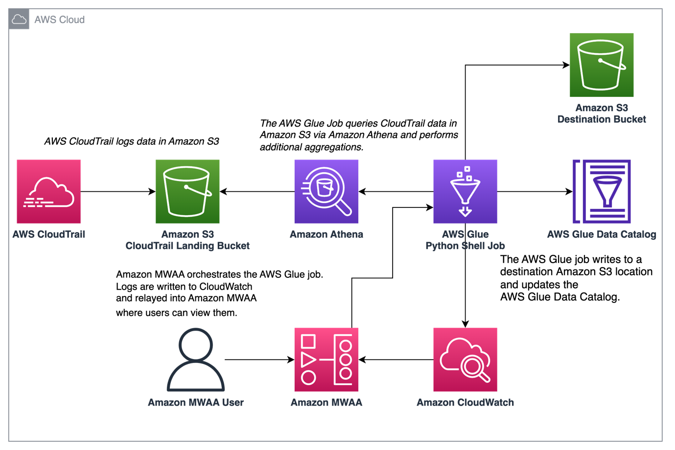
Prerequisites
You need the following prerequisites:
- Access to the console via a user with permissions to create AWS Glue jobs, create AWS Identity and Access Management (IAM) roles and policies, and manage or launch an Amazon MWAA environment
- Amazon Athena configured with a workgroup
- AWS CloudTrail set up with a trail logging into an Amazon Simple Storage Service (Amazon S3) bucket
Set up the Amazon MWAA environment
For instructions on creating your environment, refer to Create an Amazon MWAA environment. For existing users, we recommend upgrading to version 2.4.3 to take advantage of the observability enhancements featured in this post.
The steps to upgrade Amazon MWAA to version 2.4.3 differ depending on whether the current version is 1.10.12 or 2.2.2. We discuss both options in this post.
Prerequisites for setting up an Amazon MWAA environment
You must meet the following prerequisites:
- The Amazon MWAA environment should be version 2.2.2 or greater. In this post, we demonstrate upgrading to 2.4.3, but you can use 2.2.2 by changing the apache-airflow-providers-amazon package constraints in requirements.txt.
- The apache-airflow-providers-amazon package version should be 6.0.0 or greater.
- The Amazon MWAA execution role should have glue:StartJobRun and glue:GetJobRun permissions.
- The requirements.txt used by Amazon MWAA should include any additional Python modules your DAGs need.
Upgrade from version 1.10.12 to 2.4.3
If you’re using Amazon MWAA version 1.10.12, refer to Migrating to a new Amazon MWAA environment to upgrade to 2.4.3.
Upgrade from version 2.0.2 or 2.2.2 to 2.4.3
If you’re using Amazon MWAA environment version 2.2.2 or lower, complete the following steps:
- Create a requirements.txt for any custom dependencies with specific versions required for your DAGs.
- Upload the file to Amazon S3 in the appropriate location where the Amazon MWAA environment points to the requirements.txt for installing dependencies.
- Follow the steps in Migrating to a new Amazon MWAA environment and select version 2.4.3.
Update your DAGs
Customers who upgraded from an older Amazon MWAA environment may need to make updates to existing DAGs. In Airflow version 2.4.3, the Airflow environment will use the Amazon provider package version 6.0.0 by default. This package may include some potentially breaking changes, such as changes to operator names. For example, the AWSGlueJobOperator has been deprecated and replaced with the GlueJobOperator. To maintain compatibility, update your Airflow DAGs by replacing any deprecated or unsupported operators from previous versions with the new ones. Complete the following steps:
- Navigate to Amazon AWS Operators.
- Select the appropriate version installed in your Amazon MWAA instance (6.0.0. by default) to find a list of supported Airflow operators.
- Make the necessary changes in the existing DAG code and upload the modified files to the DAG location in Amazon S3.
Orchestrate the AWS Glue job from Airflow
This section covers the details of orchestrating an AWS Glue job within Airflow DAGs. Airflow eases the development of data pipelines with dependencies between heterogeneous systems such as on-premises processes, external dependencies, other AWS services, and more.
Orchestrate CloudTrail log aggregation with AWS Glue and Amazon MWAA
In this example, we go through a use case of using Amazon MWAA to orchestrate an AWS Glue Python Shell job that persists aggregated metrics based on CloudTrail logs.
CloudTrail enables visibility into AWS API calls that are being made in your AWS account. A common use case with this data would be to gather usage metrics on principals acting on your account’s resources for auditing and regulatory needs.
As CloudTrail events are being logged, they are delivered as JSON files in Amazon S3, which aren’t ideal for analytical queries. We want to aggregate this data and persist it as Parquet files to allow for optimal query performance. As an initial step, we can use Athena to do the initial querying of the data before doing additional aggregations in our AWS Glue job. For more information about creating an AWS Glue Data Catalog table, refer to Creating the table for CloudTrail logs in Athena using partition projection data. After we’ve explored the data via Athena and decided what metrics we want to retain in aggregate tables, we can create an AWS Glue job.
Create an CloudTrail table in Athena
First, we need to create a table in our Data Catalog that allows CloudTrail data to be queried via Athena. The following sample query creates a table with two partitions on the Region and date (called snapshot\_date). Be sure to replace the placeholders for your CloudTrail bucket, AWS account ID, and CloudTrail table name:
create external table if not exists `<<<CLOUDTRAIL\_TABLE\_NAME>>>`( `eventversion` string comment 'from deserializer', `useridentity` struct<type:string,principalid:string,arn:string,accountid:string,invokedby:string,accesskeyid:string,username:string,sessioncontext:struct<attributes:struct<mfaauthenticated:string,creationdate:string>,sessionissuer:struct<type:string,principalid:string,arn:string,accountid:string,username:string>>> comment 'from deserializer', `eventtime` string comment 'from deserializer', `eventsource` string comment 'from deserializer', `eventname` string comment 'from deserializer', `awsregion` string comment 'from deserializer', `sourceipaddress` string comment 'from deserializer', `useragent` string comment 'from deserializer', `errorcode` string comment 'from deserializer', `errormessage` string comment 'from deserializer', `requestparameters` string comment 'from deserializer', `responseelements` string comment 'from deserializer', `additionaleventdata` string comment 'from deserializer', `requestid` string comment 'from deserializer', `eventid` string comment 'from deserializer', `resources` array<struct<arn:string,accountid:string,type:string>> comment 'from deserializer', `eventtype` string comment 'from deserializer', `apiversion` string comment 'from deserializer', `readonly` string comment 'from deserializer', `recipientaccountid` string comment 'from deserializer', `serviceeventdetails` string comment 'from deserializer', `sharedeventid` string comment 'from deserializer', `vpcendpointid` string comment 'from deserializer')PARTITIONED BY ( `region` string, `snapshot\_date` string)ROW FORMAT SERDE 'com.amazon.emr.hive.serde.CloudTrailSerde' STORED AS INPUTFORMAT 'com.amazon.emr.cloudtrail.CloudTrailInputFormat' OUTPUTFORMAT 'org.apache.hadoop.hive.ql.io.HiveIgnoreKeyTextOutputFormat'LOCATION 's3://<<<CLOUDTRAIL\_BUCKET>>>/AWSLogs/<<<ACCOUNT\_ID>>>/CloudTrail/'TBLPROPERTIES ( 'projection.enabled'='true', 'projection.region.type'='enum', 'projection.region.values'='us-east-2,us-east-1,us-west-1,us-west-2,af-south-1,ap-east-1,ap-south-1,ap-northeast-3,ap-northeast-2,ap-southeast-1,ap-southeast-2,ap-northeast-1,ca-central-1,eu-central-1,eu-west-1,eu-west-2,eu-south-1,eu-west-3,eu-north-1,me-south-1,sa-east-1', 'projection.snapshot\_date.format'='yyyy/mm/dd', 'projection.snapshot\_date.interval'='1', 'projection.snapshot\_date.interval.unit'='days', 'projection.snapshot\_date.range'='2020/10/01,now', 'projection.snapshot\_date.type'='date', 'storage.location.template'='s3://<<<CLOUDTRAIL\_BUCKET>>>/AWSLogs/<<<ACCOUNT\_ID>>>/CloudTrail/${region}/${snapshot\_date}')Run the preceding query on the Athena console, and note the table name and AWS Glue Data Catalog database where it was created. We use these values later in the Airflow DAG code.
Sample AWS Glue job code
The following code is a sample AWS Glue Python Shell job that does the following:
- Takes arguments (which we pass from our Amazon MWAA DAG) on what day’s data to process
- Uses the AWS SDK for Pandas to run an Athena query to do the initial filtering of the CloudTrail JSON data outside AWS Glue
- Uses Pandas to do simple aggregations on the filtered data
- Outputs the aggregated data to the AWS Glue Data Catalog in a table
- Uses logging during processing, which will be visible in Amazon MWAA
import awswrangler as wrimport pandas as pdimport sysimport loggingfrom awsglue.utils import getResolvedOptionsfrom datetime import datetime, timedelta# Logging setup, redirects all logs to stdoutLOGGER = logging.getLogger()formatter = logging.Formatter('%(asctime)s.%(msecs)03d %(levelname)s %(module)s - %(funcName)s: %(message)s')streamHandler = logging.StreamHandler(sys.stdout)streamHandler.setFormatter(formatter)LOGGER.addHandler(streamHandler)LOGGER.setLevel(logging.INFO)LOGGER.info(f"Passed Args :: {sys.argv}")sql\_query\_template = """selectregion,useridentity.arn,eventsource,eventname,useragentfrom "{cloudtrail\_glue\_db}"."{cloudtrail\_table}"where snapshot\_date='{process\_date}'and region in ('us-east-1','us-east-2')"""required\_args = ['CLOUDTRAIL\_GLUE\_DB', 'CLOUDTRAIL\_TABLE', 'TARGET\_BUCKET', 'TARGET\_DB', 'TARGET\_TABLE', 'ACCOUNT\_ID']arg\_keys = [*required\_args, 'PROCESS\_DATE'] if '--PROCESS\_DATE' in sys.argv else required\_argsJOB\_ARGS = getResolvedOptions ( sys.argv, arg\_keys)LOGGER.info(f"Parsed Args :: {JOB\_ARGS}")# if process date was not passed as an argument, process yesterday's dataprocess\_date = ( JOB\_ARGS['PROCESS\_DATE'] if JOB\_ARGS.get('PROCESS\_DATE','NONE') != "NONE" else (datetime.today() - timedelta(days=1)).strftime("%Y-%m-%d") )LOGGER.info(f"Taking snapshot for :: {process\_date}")RAW\_CLOUDTRAIL\_DB = JOB\_ARGS['CLOUDTRAIL\_GLUE\_DB']RAW\_CLOUDTRAIL\_TABLE = JOB\_ARGS['CLOUDTRAIL\_TABLE']TARGET\_BUCKET = JOB\_ARGS['TARGET\_BUCKET']TARGET\_DB = JOB\_ARGS['TARGET\_DB']TARGET\_TABLE = JOB\_ARGS['TARGET\_TABLE']ACCOUNT\_ID = JOB\_ARGS['ACCOUNT\_ID']final\_query = sql\_query\_template.format( process\_date=process\_date.replace("-","/"), cloudtrail\_glue\_db=RAW\_CLOUDTRAIL\_DB, cloudtrail\_table=RAW\_CLOUDTRAIL\_TABLE)LOGGER.info(f"Running Query :: {final\_query}")raw\_cloudtrail\_df = wr.athena.read\_sql\_query( sql=final\_query, database=RAW\_CLOUDTRAIL\_DB, ctas\_approach=False, s3\_output=f"s3://{TARGET\_BUCKET}/athena-results",)raw\_cloudtrail\_df['ct']=1agg\_df = raw\_cloudtrail\_df.groupby(['arn','region','eventsource','eventname','useragent'],as\_index=False).agg({'ct':'sum'})agg\_df['snapshot\_date']=process\_dateLOGGER.info(agg\_df.info(verbose=True))upload\_path = f"s3://{TARGET\_BUCKET}/{TARGET\_DB}/{TARGET\_TABLE}"if not agg\_df.empty: LOGGER.info(f"Upload to {upload\_path}") try: response = wr.s3.to\_parquet( df=agg\_df, path=upload\_path, dataset=True, database=TARGET\_DB, table=TARGET\_TABLE, mode="overwrite\_partitions", schema\_evolution=True, partition\_cols=["snapshot\_date"], compression="snappy", index=False ) LOGGER.info(response) except Exception as exc: LOGGER.error("Uploading to S3 failed") LOGGER.exception(exc) raise excelse: LOGGER.info(f"Dataframe was empty, nothing to upload to {upload\_path}")The following are some key advantages in this AWS Glue job:
- We use an Athena query to ensure initial filtering is done outside of our AWS Glue job. As such, a Python Shell job with minimal compute is still sufficient for aggregating a large CloudTrail dataset.
- We ensure the analytics library-set option is turned on when creating our AWS Glue job to use the AWS SDK for Pandas library.
Create an AWS Glue job
Complete the following steps to create your AWS Glue job:
- Copy the script in the preceding section and save it in a local file. For this post, the file is called
script.py. - On the AWS Glue console, choose ETL jobs in the navigation pane.
- Create a new job and select Python Shell script editor.
- Select Upload and edit an existing script and upload the file you saved locally.
- Choose Create.

- On the Job details tab, enter a name for your AWS Glue job.
- For IAM role, choose an existing role or create a new role that has the required permissions for Amazon S3, AWS Glue, and Athena. The role needs to query the CloudTrail table you created earlier and write to an output location.
You can use the following sample policy code. Replace the placeholders with your CloudTrail logs bucket, output table name, output AWS Glue database, output S3 bucket, CloudTrail table name, AWS Glue database containing the CloudTrail table, and your AWS account ID.
{ "Version": "2012-10-17", "Statement": [ { "Action": [ "s3:List*", "s3:Get*" ], "Resource": [ "arn:aws:s3:::<<<CLOUDTRAIL\_LOGS\_BUCKET>>>/*", "arn:aws:s3:::<<<CLOUDTRAIL\_LOGS\_BUCKET>>>*" ], "Effect": "Allow", "Sid": "GetS3CloudtrailData" }, { "Action": [ "glue:Get*", "glue:BatchGet*" ], "Resource": [ "arn:aws:glue:us-east-1:<<<YOUR\_AWS\_ACCT\_ID>>>:catalog", "arn:aws:glue:us-east-1:<<<YOUR\_AWS\_ACCT\_ID>>>:database/<<<GLUE\_DB\_WITH\_CLOUDTRAIL\_TABLE>>>", "arn:aws:glue:us-east-1:<<<YOUR\_AWS\_ACCT\_ID>>>:table/<<<GLUE\_DB\_WITH\_CLOUDTRAIL\_TABLE>>>/<<<CLOUDTRAIL\_TABLE>>>*" ], "Effect": "Allow", "Sid": "GetGlueCatalogCloudtrailData" }, { "Action": [ "s3:PutObject*", "s3:Abort*", "s3:DeleteObject*", "s3:GetObject*", "s3:GetBucket*", "s3:List*", "s3:Head*" ], "Resource": [ "arn:aws:s3:::<<<OUTPUT\_S3\_BUCKET>>>", "arn:aws:s3:::<<<OUTPUT\_S3\_BUCKET>>>/<<<OUTPUT\_GLUE\_DB>>>/<<<OUTPUT\_TABLE\_NAME>>>/*" ], "Effect": "Allow", "Sid": "WriteOutputToS3" }, { "Action": [ "glue:CreateTable", "glue:CreatePartition", "glue:UpdatePartition", "glue:UpdateTable", "glue:DeleteTable", "glue:DeletePartition", "glue:BatchCreatePartition", "glue:BatchDeletePartition", "glue:Get*", "glue:BatchGet*" ], "Resource": [ "arn:aws:glue:us-east-1:<<<YOUR\_AWS\_ACCT\_ID>>>:catalog", "arn:aws:glue:us-east-1:<<<YOUR\_AWS\_ACCT\_ID>>>:database/<<<OUTPUT\_GLUE\_DB>>>", "arn:aws:glue:us-east-1:<<<YOUR\_AWS\_ACCT\_ID>>>:table/<<<OUTPUT\_GLUE\_DB>>>/<<<OUTPUT\_TABLE\_NAME>>>*" ], "Effect": "Allow", "Sid": "AllowOutputToGlue" }, { "Action": [ "logs:CreateLogGroup", "logs:CreateLogStream", "logs:PutLogEvents" ], "Resource": "arn:aws:logs:*:*:/aws-glue/*", "Effect": "Allow", "Sid": "LogsAccess" }, { "Action": [ "s3:GetObject*", "s3:GetBucket*", "s3:List*", "s3:DeleteObject*", "s3:PutObject", "s3:PutObjectLegalHold", "s3:PutObjectRetention", "s3:PutObjectTagging", "s3:PutObjectVersionTagging", "s3:Abort*" ], "Resource": [ "arn:aws:s3:::<<<ATHENA\_RESULTS\_BUCKET>>>", "arn:aws:s3:::<<<ATHENA\_RESULTS\_BUCKET>>>/*" ], "Effect": "Allow", "Sid": "AccessToAthenaResults" }, { "Action": [ "athena:StartQueryExecution", "athena:StopQueryExecution", "athena:GetDataCatalog", "athena:GetQueryResults", "athena:GetQueryExecution" ], "Resource": [ "arn:aws:glue:us-east-1:<<<YOUR\_AWS\_ACCT\_ID>>>:catalog", "arn:aws:athena:us-east-1:<<<YOUR\_AWS\_ACCT\_ID>>>:datacatalog/AwsDataCatalog", "arn:aws:athena:us-east-1:<<<YOUR\_AWS\_ACCT\_ID>>>:workgroup/primary" ], "Effect": "Allow", "Sid": "AllowAthenaQuerying" } ]}For Python version, choose Python 3.9.
- Select Load common analytics libraries.
- For Data processing units, choose 1 DPU.
- Leave the other options as default or adjust as needed.

- Choose Save to save your job configuration.
Configure an Amazon MWAA DAG to orchestrate the AWS Glue job
The following code is for a DAG that can orchestrate the AWS Glue job that we created. We take advantage of the following key features in this DAG:
- We use the DAG run configuration to pass or override parameters. In our example, we can pass an optional
process\_datevariable, which allows us to do backfills via the AWS Glue job. If it is not passed, the previous day’s data is processed. - We pass
script\_argsto theGlueJobOperator. These are passed as arguments to the AWS Glue job run where getResolvedOptions is used to retrieve them. - The AWS Glue job logs are relayed to Amazon MWAA by passing the
verbose=Trueparameter.
"""Sample DAG"""import airflow.utilsfrom airflow.providers.amazon.aws.operators.glue import GlueJobOperatorfrom airflow import DAGfrom datetime import timedeltaimport airflow.utils# allow backfills via DAG run parametersprocess\_date = '{{ dag\_run.conf.get("process\_date") if dag\_run.conf.get("process\_date") else "NONE" }}'dag = DAG( dag\_id = "CLOUDTRAIL\_LOGS\_PROCESSING", default\_args = { 'depends\_on\_past':False, 'start\_date':airflow.utils.dates.days\_ago(0), 'retries':1, 'retry\_delay':timedelta(minutes=5), 'catchup': False }, schedule\_interval = None, # None for unscheduled or a cron expression - E.G. "00 12 * * 2" - at 12noon Tuesday dagrun\_timeout = timedelta(minutes=30), max\_active\_runs = 1, max\_active\_tasks = 1 # since there is only one task in our DAG)## Log ingest. Assumes Glue Job is already createdglue\_ingestion\_job = GlueJobOperator( task\_id="<<<some-task-id>>>", job\_name="<<<GLUE\_JOB\_NAME>>>", script\_args={ "--ACCOUNT\_ID":"<<<YOUR\_AWS\_ACCT\_ID>>>", "--CLOUDTRAIL\_GLUE\_DB":"<<<GLUE\_DB\_WITH\_CLOUDTRAIL\_TABLE>>>", "--CLOUDTRAIL\_TABLE":"<<<CLOUDTRAIL\_TABLE>>>", "--TARGET\_BUCKET": "<<<OUTPUT\_S3\_BUCKET>>>", "--TARGET\_DB": "<<<OUTPUT\_GLUE\_DB>>>", # should already exist "--TARGET\_TABLE": "<<<OUTPUT\_TABLE\_NAME>>>", "--PROCESS\_DATE": process\_date }, region\_name="us-east-1", dag=dag, verbose=True)glue\_ingestion\_jobIncrease observability of AWS Glue jobs in Amazon MWAA
The AWS Glue jobs write logs to Amazon CloudWatch. With the recent observability enhancements to Airflow’s Amazon provider package, these logs are now integrated with Airflow task logs. This consolidation provides Airflow users with end-to-end visibility directly in the Airflow UI, eliminating the need to search in CloudWatch or the AWS Glue console.
To use this feature, ensure the IAM role attached to the Amazon MWAA environment has the following permissions to retrieve and write the necessary logs:
{ "Version": "2012-10-17", "Statement": [ { "Effect": "Allow", "Action": [ "logs:CreateLogGroup", "logs:CreateLogStream", "logs:PutLogEvents", "logs:GetLogEvents", "logs:GetLogRecord", "logs:DescribeLogStreams", "logs:FilterLogEvents", "logs:GetLogGroupFields", "logs:GetQueryResults", ], "Resource": [ "arn:aws:logs:*:*:log-group:airflow-243-<<<Your environment name>>>-*"--Your Amazon MWAA Log Stream Name ] } ]}If verbose=true, the AWS Glue job run logs show in the Airflow task logs. The default is false. For more information, refer to Parameters.
When enabled, the DAGs read from the AWS Glue job’s CloudWatch log stream and relay them to the Airflow DAG AWS Glue job step logs. This provides detailed insights into an AWS Glue job’s run in real time via the DAG logs. Note that AWS Glue jobs generate an output and error CloudWatch log group based on the job’s STDOUT and STDERR, respectively. All logs in the output log group and exception or error logs from the error log group are relayed into Amazon MWAA.
AWS admins can now limit a support team’s access to only Airflow, making Amazon MWAA the single pane of glass on job orchestration and job health management. Previously, users needed to check AWS Glue job run status in the Airflow DAG steps and retrieve the job run identifier. They then needed to access the AWS Glue console to find the job run history, search for the job of interest using the identifier, and finally navigate to the job’s CloudWatch logs to troubleshoot.
Create the DAG
To create the DAG, complete the following steps:
- Save the preceding DAG code to a local .py file, replacing the indicated placeholders.
The values for your AWS account ID, AWS Glue job name, AWS Glue database with CloudTrail table, and CloudTrail table name should already be known. You can adjust the output S3 bucket, output AWS Glue database, and output table name as needed, but make sure the AWS Glue job’s IAM role that you used earlier is configured accordingly.
- On the Amazon MWAA console, navigate to your environment to see where the DAG code is stored.
The DAGs folder is the prefix within the S3 bucket where your DAG file should be placed.
- Upload your edited file there.

- Open the Amazon MWAA console to confirm that the DAG appears in the table.

Run the DAG
To run the DAG, complete the following steps:
- Choose from the following options:
- Trigger DAG – This causes yesterday’s data to be used as the data to process
- Trigger DAG w/ config – With this option, you can pass in a different date, potentially for backfills, which is retrieved using
dag\_run.confin the DAG code and then passed into the AWS Glue job as a parameter

The following screenshot shows the additional configuration options if you choose Trigger DAG w/ config.

- Monitor the DAG as it runs.
- When the DAG is complete, open the run’s details.
On the right pane, you can view the logs, or choose Task Instance Details for a full view.

- View the AWS Glue job output logs in Amazon MWAA without using the AWS Glue console thanks to the
GlueJobOperatorverbose flag.

The AWS Glue job will have written results to the output table you specified.
- Query this table via Athena to confirm it was successful.

Summary
Amazon MWAA now provides a single place to track AWS Glue job status and enables you to use the Airflow console as the single pane of glass for job orchestration and health management. In this post, we walked through the steps to orchestrate AWS Glue jobs via Airflow using GlueJobOperator. With the new observability enhancements, you can seamlessly troubleshoot AWS Glue jobs in a unified experience. We also demonstrated how to upgrade your Amazon MWAA environment to a compatible version, update dependencies, and change the IAM role policy accordingly.
For more information about common troubleshooting steps, refer to Troubleshooting: Creating and updating an Amazon MWAA environment. For in-depth details of migrating to an Amazon MWAA environment, refer to Upgrading from 1.10 to 2. To learn about the open-source code changes for increased observability of AWS Glue jobs in the Airflow Amazon provider package, refer to the relay logs from AWS Glue jobs.
Finally, we recommend visiting the AWS Big Data Blog for other material on analytics, ML, and data governance on AWS.
About the Authors
 Rushabh Lokhande is a Data & ML Engineer with the AWS Professional Services Analytics Practice. He helps customers implement big data, machine learning, and analytics solutions. Outside of work, he enjoys spending time with family, reading, running, and golf.
 Ryan Gomes is a Data & ML Engineer with the AWS Professional Services Analytics Practice. He is passionate about helping customers achieve better outcomes through analytics and machine learning solutions in the cloud. Outside of work, he enjoys fitness, cooking, and spending quality time with friends and family.
 Vishwa Gupta is a Senior Data Architect with the AWS Professional Services Analytics Practice. He helps customers implement big data and analytics solutions. Outside of work, he enjoys spending time with family, traveling, and trying new food.
Amazon Managed Workflow for Apache Airflow (Amazon MWAA) is a managed service for Apache Airflow that lets you use the same familiar Apache Airflow environment to orchestrate your workflows and enjoy improved scalability, availability, and security without the operational burden of having to manage the underlying infrastructure.
In April 2023, Amazon MWAA added support for shell launch scripts for environment versions Apache Airflow 2.x and later. With this feature, you can customize the Apache Airflow environment by launching a custom shell launch script at startup to work better with existing integration infrastructure and help with your compliance needs. You can use this shell launch script to install custom Linux runtimes, set environment variables, and update configuration files. Amazon MWAA runs this script during startup on every individual Apache Airflow component (worker, scheduler, and web server) before installing requirements and initializing the Apache Airflow process.
In this post, we provide an overview of the features, explore applicable use cases, detail the steps to use it, and provide additional facts on the capabilities of this shell launch script.
Solution overview
To run Apache Airflow, Amazon MWAA builds Amazon Elastic Container Registry (Amazon ECR) images that bundle Apache Airflow releases with other common binaries and Python libraries. These images then get used by the AWS Fargate containers in the Amazon MWAA environment. You can bring in additional libraries through the requirements.txt and plugins.zip files and pass the Amazon Simple Storage Service (Amazon S3) paths as a parameter during environment creation or update.
However, this method to install packages didn’t cover all of your use cases to tailor your Apache Airflow environments. Customers asked us for a way to customize the Apache Airflow container images by specifying custom libraries, runtimes, and supported files.
Applicable use cases
The new feature adds the ability to customize your Apache Airflow image by launching a custom specified shell launch script at startup. You can use the shell launch script to perform actions such as the following:
- Install runtimes – Install or update Linux runtimes required by your workflows and connections. For example, you can install
libaioas a custom library for Oracle. - Configure environment variables – Set environment variables for the Apache Airflow scheduler, web server, and worker components. You can overwrite common variables such as
PATH,PYTHONPATH, andLD\_LIBRARY\_PATH. For example, you can setLD\_LIBRARY\_PATHto instruct Python to look for binaries in the paths that you specify. - Manage keys and tokens – Pass access tokens for your private PyPI/PEP-503 compliant custom repositories to
requirements.txtand configure security keys.
How it works
The shell script runs Bash commands at startup, so you can install using yum and other tools similar to how Amazon Elastic Cloud Compute Cloud (Amazon EC2) offers user data and shell scripts support. You can define a custom shell script with the .sh extension and place it in the same S3 bucket as requirements.txt and plugins.zip. You can define an S3 file version of the shell script during the environment creation or update via the Amazon MWAA console, API, or AWS Command Line Interface (AWS CLI). For details on how to configure the startup script, refer to Using a startup script with Amazon MWAA.
During the environment creation or update process, Amazon MWAA copies the plugins.zip, requirements.txt, shell script, and your Apache Airflow Directed Acrylic Graphs (DAGs) to the container images on the underlying Amazon Elastic Container Service (Amazon ECS) Fargate clusters. The Amazon MWAA instance extracts these contents and runs the startup script file that you specified. The startup script is run from the /usr/local/airflow/startup Apache Airflow directory as the airflow user. When it’s complete, the setup process will install the requirements.txt and plugins.zip files, followed by the Apache Airflow process associated with the container.
The following screenshot shows you the new optional Startup script file field on the Amazon MWAA console.

For monitoring and observability, you can view the output of the script in your Amazon MWAA environment’s Amazon CloudWatch log groups. To view the logs, you need to enable logging for the log group. If enabled, Amazon MWAA creates a new log stream starting with the prefix startup\_script\_exection\_ip. You can retrieve log events to verify that the script is working as expected.
You can also use Amazon MWAA local-runner to test this feature on your local development environments. You can now specify your custom startup script in the startup\_script directory in the local-runner. It’s recommended that you locally test your script before applying changes to your Amazon MWAA setup.
You can reference files that you package within plugins.zip or your DAGs folder from your startup script. This can be beneficial if you require installing Linux runtimes on a private web server from a local package. It’s also useful to be able to skip installation of Python libraries on a web server that doesn’t have access, either due to private web server mode or for libraries hosted on a private repository accessible only from your VPC, such as in the following example:
The MWAA\_AIRFLOW\_COMPONENT variable used in the script identifies each Apache Airflow scheduler, web server, and worker component that the script runs on.
Additional considerations
Keep in mind the following additional information of this feature:
- Specifying a startup shell script file is optional. You can pick a specific S3 file version of your script.
- Updating the startup script to an existing Amazon MWAA environment will lead to a restart of the environment. Amazon MWAA runs the startup script as each component in your environment restarts. Environment updates can take 10–30 minutes. We suggest using the Amazon MWAA
local-runnerto test and reduce the feedback loop. - You can make several changes to the Apache Airflow environment, such as setting non-reserved
AIRFLOW\_\_environment variables and installing custom Python libraries. For a detailed list of reserved and unreserved environment variables that you can set or update, refer to Set environment variables using a startup script. - Upgrading Apache Airflow core libraries and dependencies or Python versions is not supported. This is because there are constraints used for the base Apache Airflow configuration in Amazon MWAA that will lead to version incompatibility with different installs of the Python runtime and dependent library versions. Amazon MWAA runs validations prior to your custom startup script run to prevent Python or Apache Airflow installs from including triggering workflows.
- A failure during the startup script run results in an unsuccessful task stabilization of the underlying Amazon ECS Fargate containers. This can impact your Amazon MWAA environment’s ability to successfully create or update.
- The startup script runtime is limited to 5 minutes, after which it will automatically time out.
- To revert a startup script that is failing or is no longer required, edit your Amazon MWAA environment to reference a blank .sh file.
Conclusion
In this post, we talked about the new feature of Amazon MWAA that allows you to configure a startup shell launch script. This feature is supported on new and existing Amazon MWAA environments running Apache Airflow 2.x and above. Use this feature to install Linux runtimes, configure environment variables, and manage keys and tokens. You now have an additional option to customize your base Apache Airflow image to meet your specific needs.
For additional details and code examples on Amazon MWAA, visit the Amazon MWAA User Guide and the Amazon MWAA examples GitHub repo.
About the Authors
Parnab Basak is a Solutions Architect and a Serverless Specialist at AWS. He specializes in creating new solutions that are cloud native using modern software development practices like serverless, DevOps, and analytics. Parnab works closely in the analytics and integration services space helping customers adopt AWS services for their workflow orchestration needs.
 Vishal Vijayvargiya is a Software Engineer working on Amazon MWAA at Amazon Web Services. He is passionate about building distributed and scalable software systems. Vishal also enjoys playing badminton and cricket.
Deriving insight from data is hard. It’s even harder when your organization is dealing with silos that impede data access across different data stores. Seamless data integration is a key requirement in a modern data architecture to break down data silos. AWS Glue is a serverless data integration service that makes data preparation simpler, faster, and cheaper. You can discover and connect to over 70 diverse data sources, manage your data in a centralized data catalog, and create, run, and monitor data integration pipelines to load data into your data lakes and your data warehouses. AWS Glue for Apache Spark takes advantage of Apache Spark’s powerful engine to process large data integration jobs at scale.
AWS Glue released version 4.0 at AWS re:Invent 2022, which includes many upgrades, such as the new optimized Apache Spark 3.3.0 runtime, Python 3.10, and a new enhanced Amazon Redshift connector.
In this post, we discuss the main benefits that this new AWS Glue version brings and how it can help you build better data integration pipelines.
Spark upgrade highlights
The new version of Spark included in AWS Glue 4.0 brings a number of valuable features, which we highlight in this section. For more details, refer to Spark Release 3.3.0 and Spark Release 3.2.0.
Support for the pandas API
Support for the pandas API allows users familiar with the popular Python library to start writing distributed extract, transform, and load (ETL) jobs without having to learn a new framework API. We discuss this in more detail later in this post.
Python UDF profiling
With Python UDF profiling, now you can profile regular and pandas user-defined functions (UDFs). Calling show\_profiles() on the SparkContext to get details about the Python run was added on Spark 1 for RDD; now it also works for DataFrame Python UDFs and provides valuable information about how many calls to the UDF are made and how much time is spent on it.
For instance, to illustrate how the profiler measures time, the following example is the profile of a pandas UDF that processes over a million rows (but the pandas UDF only needs 112 calls) and sleeps for 1 second. We can use the command spark.sparkContext.show\_profiles(), as shown in the following screenshot.
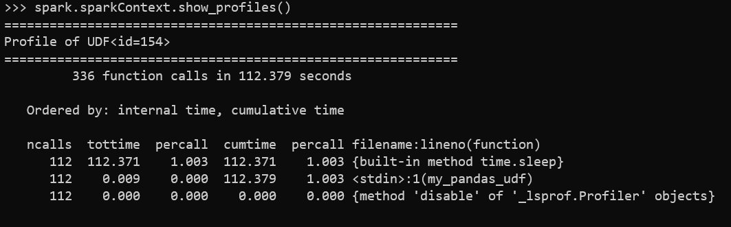
Pushdown filters
Pushdown filters are used in more scenarios, such as aggregations or limits. The upgrade also offers support for Bloom filters and skew optimization. These improvements allow for handling larger datasets by reading less data and processing it more efficiently. For more information, refer to Spark Release 3.3.0.
ANSI SQL
Now you can ask SparkSQL to follow the ANSI behavior on those points that it traditionally differed from the standard. This helps users bring their existing SQL skills and start producing value on AWS Glue faster. For more information, refer to ANSI Compliance.
Adaptive query execution by default
Adaptive query execution (AQE) by default helps optimize Spark SQL performance. You can turn AQE on and off by using spark.sql.adaptive.enabled as an umbrella configuration. Since AWS Glue 4.0, it’s enabled by default, so you no longer need to enable this explicitly.
Improved error messages
Improved error messages provide better context and easy resolution. For instance, if you have a division by zero in a SQL statement on ANSI mode, previously you would get just a Java exception: java.lang.ArithmeticException: divide by zero. Depending on the complexity and number of queries, the cause might not be obvious and might require some reruns with trial and error until it’s identified.
On the new version, you get a much more revealing error:
Not only does it show the query that caused the issue, but it also indicates the specific operation where the error occurred (the division in this case). In addition, it provides some guidance on resolving the issue.
New pandas API on Spark
The Spark upgrade brings a new, exciting feature, which is the chance to use your existing Python pandas framework knowledge in a distributed and scalable runtime. This lowers the barrier of entry for teams without previous Spark experience, so they can start delivering value quickly and make the most of the AWS Glue for Spark runtime.
The new API provides a pandas DataFrame-compatible API, so you can use existing pandas code and migrate it to AWS Glue for Spark changing the imports, although it’s not 100% compatible.
If you just want to migrate existing pandas code to run on pandas on Spark, you could replace the import and test:
In some cases, you might want to use multiple implementations on the same script, for instance because a feature is still not available on the pandas API for Spark or the data is so small that some operations are more efficient if done locally rather than distributed. In that situation, to avoid confusion, it’s better to use a different alias for the pandas and the pandas on Spark module imports, and to follow a convention to name the different types of DataFrames, because it has implications in performance and features, for instance, pandas DataFrame variables starting with pdf\_, pandas on Spark as psdf\_, and standard Spark as sdf\_ or just df\_.
You can also convert to a standard Spark DataFrame calling to\_spark(). This allows you to use features not available on pandas such as writing directly to catalog tables or using some Spark connectors.
The following code shows an example of combining the different types of APIs:
Improved Amazon Redshift connector
A new version of the Amazon Redshift connector brings many improvements:
- Pushdown optimizations
- Support for reading SUPER columns
- Writing allowed based on column names instead of position
- An optimized serializer to increase performance when reading from Amazon Redshift
- Other minor improvements like trimming pre- and post-actions and handling numeric time zone formats
This new Amazon Redshift connector is built on top of an existing open-source connector project and offers further enhancements for performance and security, helping you gain up to 10 times faster application performance. It accelerates AWS Glue jobs when reading from Amazon Redshift, and also enables you to run data-intensive workloads more reliably. For more details, see Moving data to and from Amazon Redshift. To learn more about how to use it, refer to New – Amazon Redshift Integration with Apache Spark.
When you use the new Amazon Redshift connector on an AWS Glue DynamicFrame, use the existing methods: GlueContext.create\_data\_frame and GlueContext.write\_data\_frame.
When you use the new Amazon Redshift connector on a Spark DataFrame, use the format io.github.spark\_redshift\_community.spark.redshift, as shown in the following code snippet:
Other upgrades and improvements
The following are updates and improvements in the dependent libraries:
- Spark 3.3.0-amzn-1
- Hadoop 3.3.0-amzn-0
- Hive 2.3.9-amzn-2
- Parquet 1.12
- Log4j 2
- Python 3.10
- Arrow 7.0.0
- Boto3 1.26
- EMRFS 2.54.0
- AWS Glue Data Catalog client 3.7.0
- New versions of the provided JDBC drivers:
- MySQL 8.0.23
- PostgreSQL 42.3.6
- Microsoft SQL Server 9.4.0
- Oracle 21.7
- MongoDB 4.7.2
- Amazon Redshift redshift-jdbc42-2.1.0.9
- Integrated and upgraded plugins to popular table formats:
- Iceberg 1.0.0
- Hudi 0.12.1
- Delta Lake 2.1.0
To learn more, refer to the appendices in Migrating AWS Glue jobs to AWS Glue version 4.0.
Improved performance
In addition to all the new features, AWS Glue 4.0 brings performance improvements at lower cost. In summary, AWS Glue 4.0 with Amazon Simple Storage Service (Amazon S3) is 2.7 times faster than AWS Glue 3.0, and AWS Glue 4.0 with Amazon Redshift is 7.1 times faster than AWS Glue 3.0. In the following sections, we provide details about AWS Glue 4.0 performance results with Amazon S3 and Amazon Redshift.
Amazon S3
The following chart shows the total job runtime for all queries (in seconds) in the 3 TB query dataset between AWS Glue 3.0 and AWS Glue 4.0. The TPC-DS dataset is located in an S3 bucket in Parquet format, and we used 30 G.2X workers in AWS Glue. We observed that our TPC-DS tests on Amazon S3 had a total job runtime on AWS Glue 4.0 that was 2.7 times faster than that on AWS Glue 3.0. Detailed instructions are explained in the appendix of this post.
| . | AWS Glue 3.0 | AWS Glue 4.0 |
| Total Query Time | 5084.94274 | 1896.1904 |
| Geometric Mean | 14.00217 | 10.09472 |
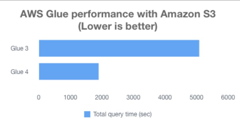
Amazon Redshift
The following chart shows the total job runtime for all queries (in seconds) in the 1 TB query dataset between AWS Glue 3.0 and AWS Glue 4.0. The TPC-DS dataset is located in a five-node ra3.4xlarge Amazon Redshift cluster, and we used 150 G.2X workers in AWS Glue. We observed that our TPC-DS tests on Amazon Redshift had a total job runtime on AWS Glue 4.0 that was 7.1 times faster than that on AWS Glue 3.0.
| . | AWS Glue 3.0 | AWS Glue 4.0 |
| Total Query Time | 22020.58 | 3075.96633 |
| Geometric Mean | 142.38525 | 8.69973 |

Get started with AWS Glue 4.0
You can start using AWS Glue 4.0 via AWS Glue Studio, the AWS Glue console, the latest AWS SDK, and the AWS Command Line Interface (AWS CLI).
To start using AWS Glue 4.0 in AWS Glue Studio, open the AWS Glue job and on the Job details tab, choose the version Glue 4.0 – Supports spark 3.3, Scala 2, Python 3.

To migrate your existing AWS Glue jobs from AWS Glue 0.9, 1.0, 2.0, and 3.0 to AWS Glue 4.0, see Migrating AWS Glue jobs to AWS Glue version 4.0.
The AWS Glue 4.0 Docker images are now available on Docker Hub, so you can use them to develop locally for the new version. Refer to Develop and test AWS Glue version 3.0 and 4.0 jobs locally using a Docker container for further details.
Conclusion
In this post, we discussed the main upgrades provided by the new 4.0 version of AWS Glue. You can already start writing new jobs on that version and benefit from all the improvements, as well as migrate your existing jobs.
About the authors
 Gonzalo Herreros is a Senior Big Data Architect on the AWS Glue team. He’s been an Apache Spark enthusiast since version 0.8. In his spare time, he likes playing board games.
 Noritaka Sekiyama is a Principal Big Data Architect on the AWS Glue team. He works based in Tokyo, Japan. He is responsible for building software artifacts to help customers. In his spare time, he enjoys cycling with his road bike.
 Bo Li is a Senior Software Development Engineer on the AWS Glue team. He is devoted to designing and building end-to-end solutions to address customer’s data analytic and processing needs with cloud-based data-intensive technologies.
 Rajendra Gujja is a Senior Software Development Engineer on the AWS Glue team. He is passionate about distributed computing and everything and anything about the data.
 Savio Dsouza is a Software Development Manager on the AWS Glue team. His team works on solving challenging distributed systems problems for data integration on Glue platform for customers using Apache Spark.
 Mohit Saxena is a Senior Software Development Manager on the AWS Glue team. His team works on distributed systems for building data lakes on AWS and simplifying integration with data warehouses for customers using Apache Spark.
Appendix: TPC-DS benchmark on AWS Glue against a dataset on Amazon S3
To perform a TPC-DS benchmark on AWS Glue against a dataset in an S3 bucket, you need to copy the TPC-DS dataset into your S3 bucket. These instructions are based on emr-spark-benchmark:
- Create a new S3 bucket in your test account if needed. In the following code, replace
$YOUR\_S3\_BUCKETwith your S3 bucket name. We suggest you exportYOUR\_S3\_BUCKETas an environment variable:
- Copy the TPC-DS source data as input to your S3 bucket. If it’s not exported as an environment variable, replace
$YOUR\_S3\_BUCKETwith your S3 bucket name:
- Build the benchmark application following the instructions in Steps to build spark-benchmark-assembly application.
For your convenience, we have provided the sample application JAR file spark-benchmark-assembly-3.3.0.jar, which we built for AWS Glue 4.0.
- Upload the spark-benchmar-assembly JAR file to your S3 bucket.
- In AWS Glue Studio, create a new AWS Glue job through the script editor:
- Under Job details, for Type, choose Spark.
- For Glue version, choose Glue 4.0 – Supports spark 3.3, Scala 2, Python 3.
- For Language, choose Scala.
- For Worker type, choose your preferred worker type.
- For Requested number of workers, choose your preferred number.
- Under Advanced properties, for Dependent JARs path, enter your S3 path for the
spark-benchmark-assemblyJAR file. - For Script, enter the following code snippet:
- Save and run the job.
The result file will be stored under s3://YOUR\_S3\_BUCKET/blog/GLUE\_TPCDS-TEST-3T-RESULT/.
This is a guest post by Kenta Oda from SOFTBRAIN Co., Ltd.
Softbrain is a leading Japanese producer of software for sales force automation (SFA) and customer relationship management (CRM). Our main product, e-Sales Manager (eSM), is an SFA/CRM tool that provides sales support to over 5,500 companies in Japan. We provide our sales customers with a one-stop source for information and visualization of sales activity, improving their efficiency and agility, which leads to greater business opportunity.
With increasing demand from our customers for analyzing data from different angles throughout the sales process, we needed an embedded analytics tool. We chose Amazon QuickSight, a cloud-native business intelligence (BI) tool that allows you to embed insightful analytics into any application with customized, interactive visuals and dashboards. It integrates seamlessly with eSM and is easy to use at a low cost.
In this post, we discuss how QuickSight is helping us provide our sales customers with the insights they need, and why we consider this business decision a win for Softbrain.
There were four things we were looking for in an embedded analytics solution:
- Rich visualization – With our previous solution, which was built in-house, there were only four types of visuals, so it was difficult to combine multiple graphs for an in-depth analysis.
- Development speed – We needed to be able to quickly implement BI functionalities. QuickSight requires minimal development due to its serverless architecture, embedding, and API.
- Cost – We moved from Tableau to QuickSight because QuickSight allowed us to provide data analysis and visualizations to our customers at a competitive price—ensuring that more of our customers can afford it.
- Ease of use – QuickSight is cloud-based and has an intuitive UX for our sales customers to work with.
Innovating with QuickSight
Individual productivity must be greatly improved to keep up with the shifting labor market in Japan. At Softbrain, we aim to innovate using the latest technology to provide science-based insights into customer and sales interactions, enabling those who use eSM to be much more productive. Sales reps and managers are able to make informed decisions.
By using QuickSight as our embedded analytics solution, we can offer data visualizations at a much lower price point, making it much more accessible for our customers than we could with other BI solutions. When we combine the process management system offered by eSM with the intuitive user experience and rich visualization capability of QuickSight, we empower customers to understand their sales data, which sits in Amazon Simple Storage Service (Amazon S3) and Amazon Aurora, and act on it.
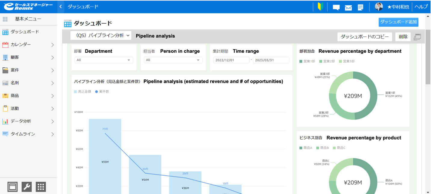
Seamless console embedding
What sets QuickSight apart from other BI tools is console embedding, which means our customers have the ability to build their own dashboards within eSM. They can choose which visualizations they want and take an in-depth look at their data. Sales strategy requires agility, and our customers need more than a fixed dashboard. QuickSight offers freedom and flexibility with console embedding.
Console embedding allows eSM to be a one-stop source for all the information sales reps and managers need. They can access all the analyses they need to make decisions right from their web browser because QuickSight is fully managed and serverless. With other BI solutions, the user would need to have the client application installed on their computer to create their own dashboards.

Empowering our sales customers
With insights from QuickSight embedded into eSM, sales reps can analyze the gap between their budget and actual revenue to build an action plan to fill the gap. They can use their dashboards to analyze data on a weekly and monthly basis. They can share this information at meetings and explore the data to figure out why there might be low attainment for certain customers. Our customers can use eSM and QuickSight to understand why win or loss opportunities are increasing. Managers can analyze and compare the performance of their sales reps to learn what high-performing reps are doing and help low performers. Sales reps can also evaluate their own performance.
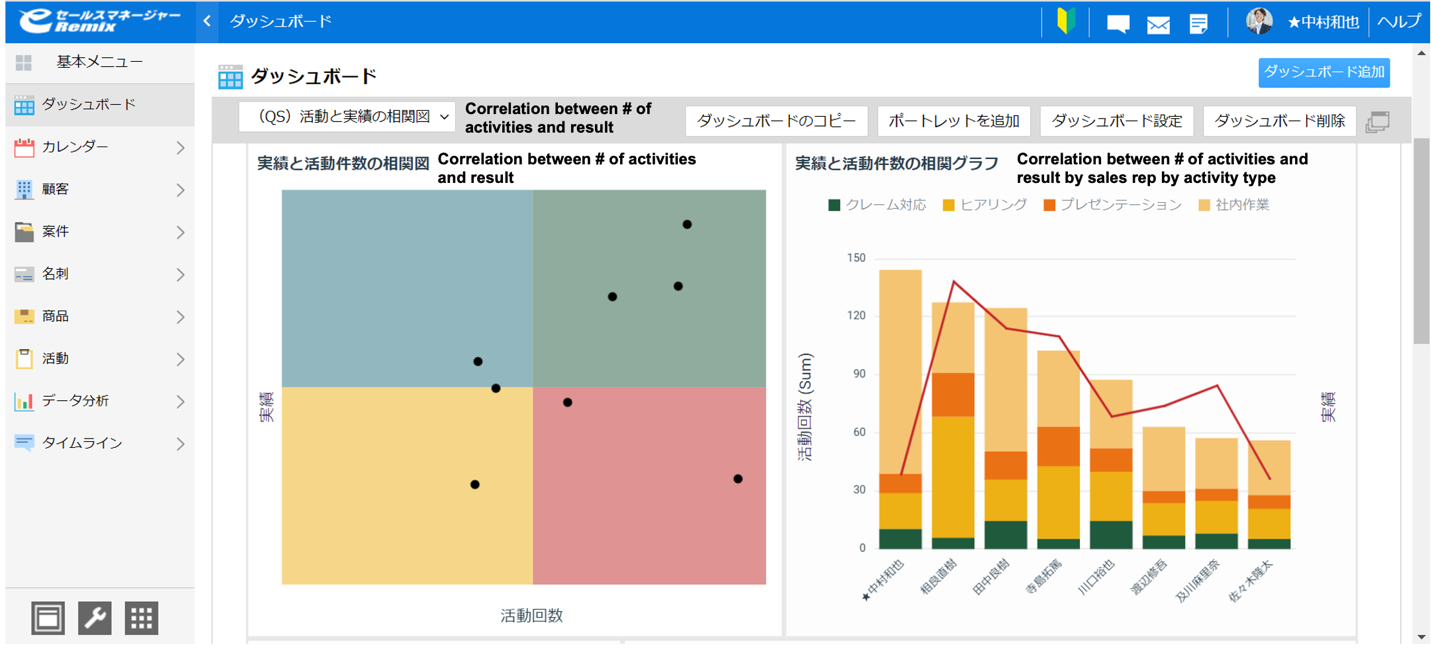
Driving 95% customer retention rate
All of these insights come from putting sales data into eSM and QuickSight. It’s no secret that our customers love QuickSight. We can boast a 95% customer retention rate and offer QuickSight as an embedded BI solution at largest scale in Japan.
To learn more about how you can embed customized data visuals and interactive dashboards into any application, visit Amazon QuickSight Embedded.
About the author
 Kenta Oda is the Chief Technology Officer at SOFTBRAIN Co., Ltd. He is in responsible of new product development with keen insight on better customer experience and go-to-market strategy.
Customers are adopting Amazon Managed Service for Apache Kafka (Amazon MSK) as a fast and reliable streaming platform to build their enterprise data hub. In addition to streaming capabilities, setting up Amazon MSK enables organizations to use a pub/sub model for data distribution with loosely coupled and independent components.
To publish and distribute the data between Apache Kafka clusters and other external systems including search indexes, databases, and file systems, you’re required to set up Apache Kafka Connect, which is the open-source component of Apache Kafka framework, to host and run connectors for moving data between various systems. As the number of upstream and downstream applications grow, so does the complexity to manage, scale, and administer the Apache Kafka Connect clusters. To address these scalability and manageability concerns, Amazon MSK Connect provides the functionality to deploy fully managed connectors built for Apache Kafka Connect, with the capability to automatically scale to adjust with the workload changes and pay only for the resources consumed.
In this post, we walk through a solution to stream data from Amazon Relation Database Service (Amazon RDS) for MySQL to an MSK cluster in real time by configuring and deploying a connector using Amazon MSK Connect.
Solution overview
For our use case, an enterprise wants to build a centralized data repository that has multiple producer and consumer applications. To support streaming data from applications with different tools and technologies, Amazon MSK is selected as the streaming platform. One of the primary applications that currently writes data to Amazon RDS for MySQL would require major design changes to publish data to MSK topics and write to the database at the same time. Therefore, to minimize the design changes, this application would continue writing the data to Amazon RDS for MySQL with the additional requirement to synchronize this data with the centralized streaming platform Amazon MSK to enable real-time analytics for multiple downstream consumers.
To solve this use case, we propose the following architecture that uses Amazon MSK Connect, a feature of Amazon MSK, to set up a fully managed Apache Kafka Connect connector for moving data from Amazon RDS for MySQL to an MSK cluster using the open-source JDBC connector from Confluent.

Set up the AWS environment
To set up this solution, you need to create a few AWS resources. The AWS CloudFormation template provided in this post creates all the AWS resources required as prerequisites:
- An Amazon Virtual Private Cloud (Amazon VPC) network with three private subnets and one public subnet
- The required internet gateway, Network Address Translation (NAT) gateway, security groups, and route tables for the necessary incoming and outgoing traffic flow
- AWS Identity and Access Management (IAM) roles and policies required for authentication and authorization between different AWS services
- An Amazon Simple Storage Service (Amazon S3) bucket to store the open-source Confluent JDBC connector JAR files
- An RDS for MySQL DB instance to act as the source for the streaming data flow
- An MSK cluster to act as the target for the streaming data flow
- An Amazon Elastic Compute Cloud (Amazon EC2) instance to act as the Kafka client and MySQL client for various administration and data validation tasks
The following table lists the parameters you must provide for the template.
| Parameter Name | Description | Keep Default Value |
| Stack name | Name of CloudFormation stack. | No |
| DBInstanceID | Name of RDS for MySQL instance. | No |
| DBName | Database name to store sample data for streaming. | Yes |
| DBInstanceClass | Instance type for RDS for MySQL instance. | No |
| DBAllocatedStorage | Allocated size for DB instance (GiB). | No |
| DBUsername | Database user for MySQL database access. | No |
| DBPassword | Password for MySQL database access. | No |
| JDBCConnectorPluginBukcetName | Bucket for storing MSK Connect connector JAR files and plugin. | No |
| ClientIPCIDR | IP address of client machine to connect to EC2 instance. | No |
| EC2KeyPair | Key pair to be used in your EC2 instance. This EC2 instance will be used as a proxy to connect from your local machine to the EC2 client instance. | No |
| EC2ClientImageId | Latest AMI ID of Amazon Linux 2. You can keep the default value for this post. | Yes |
| VpcCIDR | IP range (CIDR notation) for this VPC. | No |
| PrivateSubnetOneCIDR | IP range (CIDR notation) for the private subnet in the first Availability Zone. | No |
| PrivateSubnetTwoCIDR | IP range (CIDR notation) for the private subnet in the second Availability Zone. | No |
| PrivateSubnetThreeCIDR | IP range (CIDR notation) for the private subnet in the third Availability Zone. | No |
| PublicSubnetCIDR | IP range (CIDR notation) for the public subnet. | No |
To launch the CloudFormation stack, choose Launch Stack:
After the CloudFormation template is complete and the resources are created, the Outputs tab shows the resource details.

Validate sample data in the RDS for MySQL instance
To prepare the sample data for this use case, complete the following steps:
- SSH into the EC2 client instance MSKEC2Client using the following command from your local terminal:
- Run the following commands to validate the data has been loaded successfully:

Synchronize all tables’ data from Amazon RDS to Amazon MSK
To sync all tables from Amazon RDS to Amazon MSK, create an Amazon MSK Connect managed connector with the following steps:
- On the Amazon MSK console, choose Custom plugins in the navigation pane under MSK Connect.
- Choose Create custom plugin.
- For S3 URI – Custom plugin object, browse to the ZIP file named confluentinc-kafka-connect-jdbc-plugin.zip (created by the CloudFormation template) for the JDBC connector in the S3 bucket
bkt-msk-connect-plugins-<aws\_account\_id>. - For Custom plugin name, enter
msk-confluent-jdbc-plugin-v1. - Enter an optional description.
- Choose Create custom plugin.

After the custom plugin has been successfully created, it will be available in Active status

- Choose Connectors in the navigation pane under MSK Connect.
- Choose Create connector.
- Select Use existing custom plugin and under Custom plugins, select the plugin
msk-confluent-jdbc-plugin-v1that you created earlier. - Choose Next.

- For Connector name, enter
msk-jdbc-connector-rds-to-msk. - Enter an optional description.
- For Cluster type, select MSK cluster.

- For MSK clusters, select the cluster you created earlier.
- For Authentication, choose IAM.
- Under Connector configurations, enter the following settings:
The following table provides a brief summary of all the preceding configuration options.
| Configuration Options | Description |
| connector.class | JAVA class for the connector |
| connection.user | User name to authenticate with the MySQL endpoint |
| connection.url | JDBC URL identifying the hostname and port number for the MySQL endpoint |
| connection.password | Password to authenticate with the MySQL endpoint |
| tasks.max | Maximum number of tasks to be launched for this connector |
| poll.interval.ms | Time interval in milliseconds between subsequent polls for each table to pull new data |
| topic.prefix | Custom prefix value to append with each table name when creating topics in the MSK cluster |
| mode | The operation mode for each poll, such as bulk, timestamp, incrementing, or timestamp+incrementing |
| connection.attempts | Maximum number of retries for JDBC connection |
| security.protocol | Sets up TLS for encryption |
| sasl.mechanism | Identifies the SASL mechanism to use |
| ssl.truststore.location | Location for storing trusted certificates |
| ssl.keystore.location | Location for storing private keys |
| sasl.client.callback.handler.class | Encapsulates constructing a SigV4 signature based on extracted credentials |
| sasl.jaas.config | Binds the SASL client implementation |

- In the Connector capacity section, select Autoscaled for Capacity type and keep the default value of 1 for MCU count per worker.
- Set 4 for Maximum number of workers and keep all other default values for Workers and Autoscaling utilization thresholds.

- For Worker configuration, select Use the MSK default configuration.
- Under Access permissions, choose the custom IAM role
msk-connect-rds-jdbc-MSKConnectServiceIAMRole-*created earlier.

- For Log delivery, select Deliver to Amazon CloudWatch Logs.
- For Log group, choose the log group
msk-jdbc-source-connectorcreated earlier.

- Choose Next.
- Under Review and Create, validate all the settings and choose Create connector.
After the connector has transitioned to RUNNING status, the data should start flowing from the RDS instance to the MSK cluster.

Validate the data
To validate and compare the data, complete the following steps:
- SSH into the EC2 client instance
MSKEC2Clientusing the following command from your local terminal: - To connect to the MSK cluster with IAM authentication, enter the latest version of the aws-msk-iam-auth JAR file in the class path:
- On the Amazon MSK console, choose Clusters in the navigation pane and choose the cluster
MSKConnect-msk-connect-rds-jdbc. - On the Cluster summary page, choose View client information.

- In the View client information section, under Bootstrap servers, copy the private endpoint for Authentication type IAM.

- Set up additional environment variables for working with the latest version of Apache Kafka installation and connecting to Amazon MSK bootstrap servers, where
<bootstrap servers>is the list of bootstrap servers that allow connecting to the MSK cluster with IAM authentication: - Set up a config file named
client/propertiesto be used for authentication: - Validate the list of topics created in the MSK cluster:

- Validate that data has been loaded to the topics in the MSK cluster:

Synchronize data using a query to Amazon RDS and write to Amazon MSK
To synchronize the results of a query that flattens data by joining multiple tables in Amazon RDS for MySQL, create an Amazon MSK Connect managed connector with the following steps:
- On Amazon MSK console, choose Connectors in the navigation pane under MSK Connect.
- Choose Create connector.
- Select Use existing custom plugin and under Custom plugins, select the
pluginmsk-confluent-jdbc-plugin-v1. - For Connector name, enter
msk-jdbc-connector-rds-to-msk-query. - Enter an optional description.
- For Cluster type, select MSK cluster.
- For MSK clusters, select the cluster you created earlier.
- For Authentication, choose IAM.
- Under Connector configurations, enter the following settings:
- In the Connector capacity section, select Autoscaled for Capacity type and keep the default value of 1 for MCU count per worker.
- Set 4 for Maximum number of workers and keep all other default values for Workers and Autoscaling utilization thresholds.
- For Worker configuration, select Use the MSK default configuration.
- Under Access permissions, choose the custom IAM role
role\_msk\_connect\_serivce\_exec\_custom. - For Log delivery, select Deliver to Amazon CloudWatch Logs.
- For Log group, choose the log group created earlier.
- Choose Next.
- Under Review and Create, validate all the settings and choose Create connector.
Once the connector has transitioned to RUNNING status, the data should start flowing from the RDS instance to the MSK cluster.

- For data validation, SSH into the EC2 client instance MSKEC2Client and run the following command to see the data in the topic:

Clean up
To clean up your resources and avoid ongoing charges, complete the following the steps:
- On the Amazon MSK console, choose Connectors in the navigation pane under MSK Connect.
- Select the connectors you created and choose Delete.

- On the Amazon S3 console, choose Buckets in the navigation pane.
- Search for the bucket with the naming convention
bkt-msk-connect-plugins-<aws\_account\_id>. - Delete all the folders and objects in this bucket.
- Delete the bucket after all contents have been removed.
- To delete all other resources created using the CloudFormation stack, delete the stack via the AWS CloudFormation console.
Conclusion
Amazon MSK Connect is a fully managed service that provisions the required resources, monitors the health and delivery state of connectors, maintains the underlying hardware, and auto scales connectors to balance the workloads. In this post, we saw how to set up the open-source JDBC connector from Confluent to stream data between an RDS for MySQL instance and an MSK cluster. We also explored different options to synchronize all the tables as well as use the query-based approach to stream denormalized data into the MSK topics.
For more information about Amazon MSK Connect, see Getting started using MSK Connect.
About the Authors
 Manish Virwani is a Sr. Solutions Architect at AWS. He has more than a decade of experience designing and implementing large-scale big data and analytics solutions. He provides technical guidance, design advice, and thought leadership to some of the key AWS customers and partners.
 Indira Balakrishnan is a Principal Solutions Architect in the AWS Analytics Specialist SA Team. She is passionate about helping customers build cloud-based analytics solutions to solve their business problems using data-driven decisions. Outside of work, she volunteers at her kids’ activities and spends time with her family.
If you want to learn how to make the most of your company’s data, especially during today’s uncertain times, don’t miss AWS Data Insights Day on May 24, 2023. Learn more.

Credit: Phil Goldstein
Jerry Wang, Peloton’s Director of Data Engineering (left), and Evy Kho, Peloton’s Manager of Subscription Analytics, discuss how the company has benefited from using Amazon Redshift.
New York-based Peloton, which aims to help people around the world reach their fitness goals through its connected fitness equipment and subscription-based classes, saw booming growth in the early stage of the COVID-19 pandemic. In 2020, as gyms shuttered and people looked for ways to stay active from the safety of their homes, the company’s annual revenue soared from $915 million in 2019 to $4 billion in 2021. Meanwhile, the company’s subscribers jumped from around 360,000 in 2019 to 2.76 million at the end of 2022.
As Peloton’s business continued to evolve amid a changing macroeconomic environment, it was essential that it could make smart business decisions quickly, and one of the best ways to do that was to harness insights from the huge amount of data that it had been gathering over recent years.
During that same time, AWS has been focused on helping customers manage their ever-growing volumes of data with tools like Amazon Redshift, the first fully managed, petabyte-scale cloud data warehouse. The service has grown into a multifaceted service used by tens of thousands of customers to process exabytes of data on a daily basis (1 exabyte is equivalent to 119 billion song downloads). With Amazon Redshift, you get access to a modern data architecture that helps you break down internal data silos, share data securely and seamlessly, and support multiple users who don’t have specialized data and analytics skills.
When Jerry Wang, Peloton’s director of data engineering, joined the company in 2019, he needed to make sure the service would handle the company’s massive and growing amounts of data. He also needed to ensure Amazon Redshift could help the company efficiently manage the wide variety of data and the users who would need to access it, and deliver insights on that data at high velocity—all while being cost-effective and secure.
Wang was delighted to see that as Peloton experienced its massive growth and change, AWS continued to release new Amazon Redshift features and associated capabilities that would perfectly suit his company’s needs at just the right time.
“Over the years, I’ve always been in the stage where I hope Redshift can have a new, specific feature,” Wang says, “and then, in a very limited amount of time, AWS releases that kind of feature.”
Peloton’s data volumes soar as the business grows

Credit: Peloton
As Peloton’s business has evolved, the amount of data it is generating and analyzing has grown exponentially. From 2019 to now, Wang reports the amount of data the company holds has grown by a factor of 20. In fact, a full 95% of the total historical data the company has generated has come in the last 4 years. This growth has been driven both by surges in the number of users on Peloton’s platform and the variety of data the company is collecting.
Peloton collects reams of data on its sales of internet-connected exercise equipment like stationary bikes and treadmills. The company also collects data on customers’ workouts, which it then provides back to them in various reports such as a monthly summary, giving them insights into how often they worked out, their best output, trends in their workouts, the instructor they used the most, how many calories they burned, and more. All of this data helps Peloton make strategic business decisions, refine its operations to become more efficient, adjust its programming, and drive subscriber engagement and growth.
In 2019 and into 2020, as Peloton’s business boomed, the company needed an analytics system that could help it manage an explosion of data, both from users and related to its business. The company embraced Amazon Redshift because of the service’s versatility, ease of use, price-performance at scale, continuous pace of innovation, and ability to handle concurrent queries from dozens of internal data teams.
Wang said that when he joined the company, there were two kinds of users who were performing daily data operations in Peloton’s Amazon Redshift data warehouse. One group performed extract, transform, and load (ETL) operations to take raw data and make it available for analysis. The other was a group of business users who, each morning, would perform queries to generate local data visualizations, creating a surge of capacity on the Amazon Redshift data warehouse. “So, when these two loads ran together, the performance suffered directly,” Wang says.
One of the features Peloton adopted was Amazon Redshift Concurrency Scaling, which provides consistent and fast query performance even across thousands of concurrent users and concurrent queries. This helped solve the problem by automatically adding query processing power in seconds and processing queries without delays. When the workload demand subsided, the extra processing power was automatically removed, so Peloton only had to pay for the time when Concurrency Scaling data warehouses were in use. Wang says Peloton was running about 10 hours of Concurrency Scaling on a consistent daily basis to deal with the congestion, which, he says, “solved my problem at that moment.”
In 2020, as the pandemic inspired hoards to hop on bikes in their living rooms, Wang also upgraded Amazon Redshift with the newly introduced Amazon Redshift RA3 instances with managed storage (RMS). These represented a new generation of compute instances with managed, analytics-optimized storage designed for high-transaction, fast query performance and lower costs.
“The new instance … was a great feature for us,” Wang says. “It solved our concern about moving from terabyte scale to petabyte scale.”
Peloton’s business is driven by a variety of data for a wide range of users

Credit: Peloton
Peloton’s business model is driven by a wide variety of large volumes of data. In addition to selling bikes, treadmills, and indoor rowing machines, and expanding its subscription platform to include non-equipment-based workouts, the company has dozens of instructors in five countries, and it licenses music from three major music licensors. In 2022, it began renting bikes as well as selling them. Internally, Peloton employees working in finance, accounting, marketing, supply chain operations, music and content, and more are using data to track subscriber growth, content engagement, and which sales channels are leading to the most net new subscriptions.
“There was a time when we were just a bike company, and now we’re so much more than that,” says Evy Kho, manager of subscription analytics at Peloton.
There is also a much wider range of sales channels for Peloton equipment than just a few years ago. In the past, Peloton customers could only purchase bikes through the Peloton website or secondhand. Now, customers can purchase hardware from third-party sites like Amazon. That introduced “a really interesting data problem” for Peloton, says Kho, as it strives to determine how to link subscription signups back to exercise equipment sales.
In the face of this variability, complexity, and need for instant access to data to inform business decision-makers, Peloton embraced Amazon Redshift Serverless as an early adopter after AWS introduced the feature in late 2021. Redshift Serverless allows companies to quickly run and scale analytics capacity without database managers and data engineers needing to manage data warehouse infrastructure.
Redshift Serverless also has the ability to quickly spin up analytics capacity for different users, or personas, within an organization. This allows different teams across Peloton to perform analytics on the same datasets at the same time to generate insights on their individual parts of the business. It’s “incredibly important in terms of assessing what’s been good for our business,” Kho says.
Wang also says Peloton is considering supporting specific personas for those who need analytics around financial information governed by securities regulations, and another for users who need to perform analytics on data governed by regulations around personally identifiable information (PII).
Wang points out that Redshift Serverless also allows him to spin up Amazon Redshift data warehouses to handle special usage patterns. For example, ETL loads are often high I/O but require low CPU resources, and are very predictable because Peloton controls the process. However, when internal users want to perform data analytics or machine learning, the company doesn’t have control over the demand for those queries, and the load on Amazon Redshift data warehouses can be variable, with some queries more CPU-intensive than others. Previously, any provisioned data warehouse would have a fixed cost, and it would have to be provisioned to cope with the highest possible workloads even if the utilization rates turned out to be low. Now, for these different scenarios, Wang creates different Amazon Redshift instances to handle that variability without those heavy, fixed costs.
As Peloton’s use of Amazon Redshift has evolved and matured, its costs have gone down, according to Wang. “If you look at Serverless, the amount … that we spend on the Serverless is actually much smaller than we did previously, compared to the Concurrency Scaling cost.”
In a serverless environment, there is no upfront cost to Peloton. “I can set it up as quickly as I can and we pay as we need it,” Wang says. “It scales up when the load goes up. So, it’s a perfect fit.”
Peloton uses Amazon Redshift to get to insights faster

Credit: Peloton
Peloton’s focus on efficiency and sustainable growth has meant that it needs to act more quickly than ever to make sound, data-informed business decisions. Peloton, Wang notes, is long past the stage where all it cared about was growth. “We are a mature company now, so operational efficiency is very important; it’s key to the business,” he says.
When Peloton launches new products, for example, two things typically happen, Wang says. One is that there is a spike in data volumes, both in traffic to its website and the number of sales transactions it’s processing. The second is that the company’s management team will want real-time updates and analysis of how sales are performing.
Redshift Serverless and data sharing lets users quickly start performing real-time analytics and build reporting and dashboard applications without any additional engineering required. Wang confirms this benefit, especially in the example of a new product launch, saying it “will scale up by itself without me having to intervene. I don’t need to allocate a budget. I don’t need to change any configurations.”
In the past, when Peloton only offered its fitness equipment through its own website, it was easy to associate fulfillment data on orders with subscriptions. However, as those channels grew and became more complex, Peloton turned to the data sharing capabilities of Amazon Redshift to share data quickly and easily across teams. Peloton’s teams for subscriber analytics, supply chain, accounting, and more need fast access to fulfillment data to ensure they can track it accurately, respond if changes are needed, and determine how fulfillment data aligns with subscriptions and revenue.
“Getting them those results even faster has been incredibly helpful, and is only becoming more important as we have become far more data-driven than I think you could argue we were before,” Kho says.
Amazon Redshift marries data security, governance, and compliance with innovation
Like all customers, Peloton is concerned about data security, governance, and compliance. With security features like dynamic data masking, role-based access control, and row-level security, Amazon Redshift protects customers’ data with granular authorization features and comprehensive identity management.
Customers also are able to easily provide authorizations for the right users or groups. These features are available out of the box, within the standard pricing model.
Wang notes that Amazon Redshift’s security model is based on a traditional database model, which is a well-understood and robust model. “So for us, to provision access on that model is quite straightforward,” Wang says.
At every stage of Peloton’s evolution over the last 4 years, the company has been able to turn to AWS and Amazon Redshift to help it effectively manage that growth and complexity.
“When I started,” Wang says, “I said, OK, I need a temporary boost in capacity. Then came Concurrency Scaling. And then I said, I need cheaper storage, and [RA3] comes along. And then the ultimate challenge [was], I’m no longer satisfied with a monolithic Redshift instance. Serverless solved that issue.”
Join AWS Data Insights Day 2023
If you want to learn how your company can use Amazon Redshift to analyze large volumes of data in an easy-to-use, scalable, cost-effective, and secure way, don’t miss AWS Data Insights Day on May 24, 2023. During the day-long virtual event, learn from AWS leaders, experts, partners, and customers—including Peloton, Gilead, McDonald’s, Global Foundries, Schneider Electric, and Flutter Entertainment—how Amazon Redshift and features like Amazon Redshift ML are helping drive business innovation, optimization, and cost savings, especially in today’s uncertain economic times.
| Register Now |
To learn more about Amazon Redshift, see Amazon Redshift and Amazon Redshift: Ten years of continuous reinvention.
About the author
 Phil Goldstein is a copywriter and editor with AWS product marketing. He has 15 years of technology writing experience, and prior to joining AWS was a senior editor at a content marketing agency and a business journalist covering the wireless industry.
In today’s digital age, logging is a critical aspect of application development and management, but efficiently managing logs while complying with data protection regulations can be a significant challenge. Zoom, in collaboration with the AWS Data Lab team, developed an innovative architecture to overcome these challenges and streamline their logging and record deletion processes. In this post, we explore the architecture and the benefits it provides for Zoom and its users.
Application log challenges: Data management and compliance
Application logs are an essential component of any application; they provide valuable information about the usage and performance of the system. These logs are used for a variety of purposes, such as debugging, auditing, performance monitoring, business intelligence, system maintenance, and security. However, although these application logs are necessary for maintaining and improving the application, they also pose an interesting challenge. These application logs may contain personally identifiable data, such as user names, email addresses, IP addresses, and browsing history, which creates a data privacy concern.
Laws such as the General Data Protection Regulation (GDPR) and the California Consumer Privacy Act (CCPA) require organizations to retain application logs for a specific period of time. The exact length of time required for data storage varies depending on the specific regulation and the type of data being stored. The reason for these data retention periods is to ensure that companies aren’t keeping personal data longer than necessary, which could increase the risk of data breaches and other security incidents. This also helps ensure that companies aren’t using personal data for purposes other than those for which it was collected, which could be a violation of privacy laws. These laws also give individuals the right to request the deletion of their personal data, also known as the “right to be forgotten.” Individuals have the right to have their personal data erased, without undue delay.
So, on one hand, organizations need to collect application log data to ensure the proper functioning of their services, and keep the data for a specific period of time. But on the other hand, they may receive requests from individuals to delete their personal data from the logs. This creates a balancing act for organizations because they must comply with both data retention and data deletion requirements.
This issue becomes increasingly challenging for larger organizations that operate in multiple countries and states, because each country and state may have their own rules and regulations regarding data retention and deletion. For example, the Personal Information Protection and Electronic Documents Act (PIPEDA) in Canada and the Australian Privacy Act in Australia are similar laws to GDPR, but they may have different retention periods or different exceptions. Therefore, organizations big or small must navigate this complex landscape of data retention and deletion requirements, while also ensuring that they are in compliance with all applicable laws and regulations.
Zoom’s initial architecture
During the COVID-19 pandemic, the use of Zoom skyrocketed as more and more people were asked to work and attend classes from home. The company had to rapidly scale its services to accommodate the surge and worked with AWS to deploy capacity across most Regions globally. With a sudden increase in the large number of application endpoints, they had to rapidly evolve their log analytics architecture and worked with the AWS Data Lab team to quickly prototype and deploy an architecture for their compliance use case.
At Zoom, the data ingestion throughput and performance needs are very stringent. Data had to be ingested from several thousand application endpoints that produced over 30 million messages every minute, resulting in over 100 TB of log data per day. The existing ingestion pipeline consisted of writing the data to Apache Hadoop HDFS storage through Apache Kafka first and then running daily jobs to move the data to persistent storage. This took several hours while also slowing the ingestion and creating the potential for data loss. Scaling the architecture was also an issue because HDFS data would have to be moved around whenever nodes were added or removed. Furthermore, transactional semantics on billions of records were necessary to help meet compliance-related data delete requests, and the existing architecture of daily batch jobs was operationally inefficient.
It was at this time, through conversations with the AWS account team, that the AWS Data Lab team got involved to assist in building a solution for Zoom’s hyper-scale.
Solution overview
The AWS Data Lab offers accelerated, joint engineering engagements between customers and AWS technical resources to create tangible deliverables that accelerate data, analytics, artificial intelligence (AI), machine learning (ML), serverless, and container modernization initiatives. The Data Lab has three offerings: the Build Lab, the Design Lab, and Resident Architect. During the Build and Design Labs, AWS Data Lab Solutions Architects and AWS experts supported Zoom specifically by providing prescriptive architectural guidance, sharing best practices, building a working prototype, and removing technical roadblocks to help meet their production needs.
Zoom and the AWS team (collectively referred to as “the team” going forward) identified two major workflows for data ingestion and deletion.
Data ingestion workflow
The following diagram illustrates the data ingestion workflow.

The team needed to quickly populate millions of Kafka messages in the dev/test environment to achieve this. To expedite the process, we (the team) opted to use Amazon Managed Streaming for Apache Kafka (Amazon MSK), which makes it simple to ingest and process streaming data in real time, and we were up and running in under a day.
To generate test data that resembled production data, the AWS Data Lab team created a custom Python script that evenly populated over 1.2 billion messages across several Kafka partitions. To match the production setup in the development account, we had to increase the cloud quota limit via a support ticket.
We used Amazon MSK and the Spark Structured Streaming capability in Amazon EMR to ingest and process the incoming Kafka messages with high throughput and low latency. Specifically, we inserted the data from the source into EMR clusters at a maximum incoming rate of 150 million Kafka messages every 5 minutes, with each Kafka message holding 7–25 log data records.
To store the data, we chose to use Apache Hudi as the table format. We opted for Hudi because it’s an open-source data management framework that provides record-level insert, update, and delete capabilities on top of an immutable storage layer like Amazon Simple Storage Service (Amazon S3). Additionally, Hudi is optimized for handling large datasets and works well with Spark Structured Streaming, which was already being used at Zoom.
After 150 million messages were buffered, we processed the messages using Spark Structured Streaming on Amazon EMR and wrote the data into Amazon S3 in Apache Hudi-compatible format every 5 minutes. We first flattened the message array, creating a single record from the nested array of messages. Then we added a unique key, known as the Hudi record key, to each message. This key allows Hudi to perform record-level insert, update, and delete operations on the data. We also extracted the field values, including the Hudi partition keys, from incoming messages.
This architecture allowed end-users to query the data stored in Amazon S3 using Amazon Athena with the AWS Glue Data Catalog or using Apache Hive and Presto.
Data deletion workflow
The following diagram illustrates the data deletion workflow.
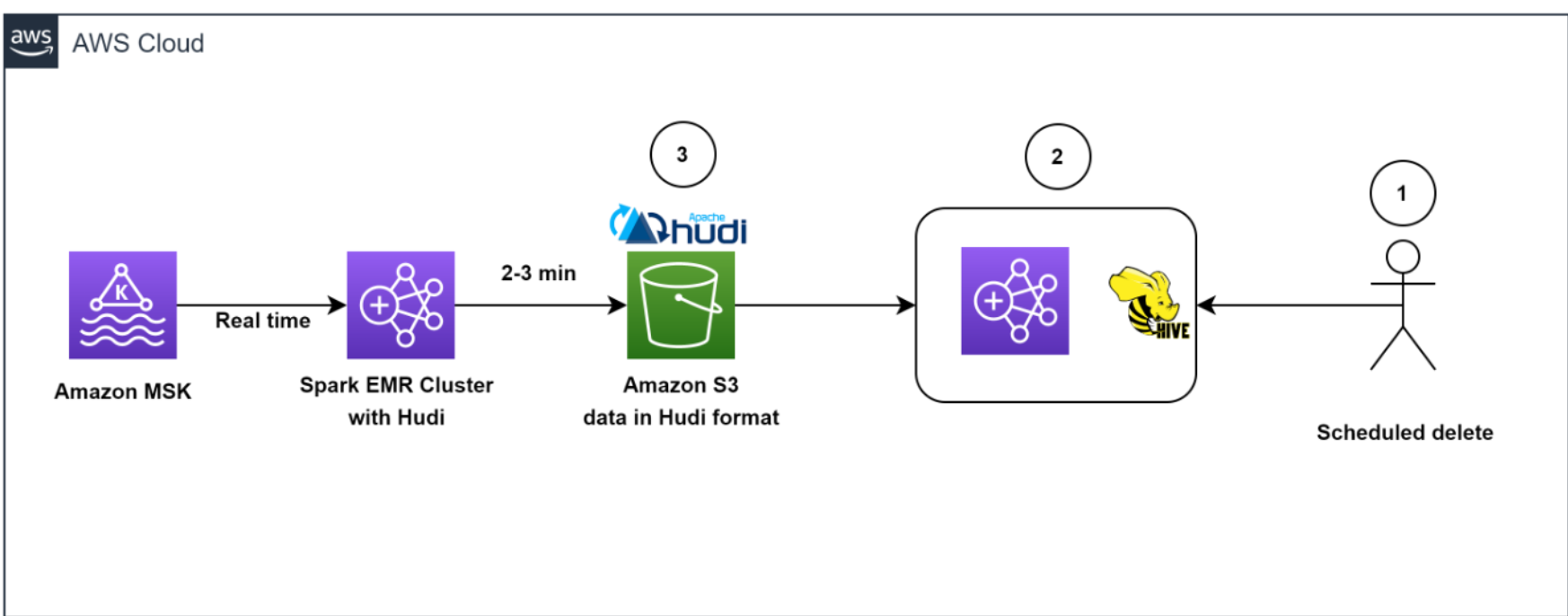
Our architecture allowed for efficient data deletions. To help comply with the customer-initiated data retention policy for GDPR deletes, scheduled jobs ran daily to identify the data to be deleted in batch mode.
We then spun up a transient EMR cluster to run the GDPR upsert job to delete the records. The data was stored in Amazon S3 in Hudi format, and Hudi’s built-in index allowed us to efficiently delete records using bloom filters and file ranges. Because only those files that contained the record keys needed to be read and rewritten, it only took about 1–2 minutes to delete 1,000 records out of the 1 billion records, which had previously taken hours to complete as entire partitions were read.
Overall, our solution enabled efficient deletion of data, which provided an additional layer of data security that was critical for Zoom, in light of its GDPR requirements.
Architecting to optimize scale, performance, and cost
In this section, we share the following strategies Zoom took to optimize scale, performance, and cost:
- Optimizing ingestion
- Optimizing throughput and Amazon EMR utilization
- Decoupling ingestion and GDPR deletion using EMRFS
- Efficient deletes with Apache Hudi
- Optimizing for low-latency reads with Apache Hudi
- Monitoring
Optimizing ingestion
To keep the storage in Kafka lean and optimal, as well as to get a real-time view of data, we created a Spark job to read incoming Kafka messages in batches of 150 million messages and wrote to Amazon S3 in Hudi-compatible format every 5 minutes. Even during the initial stages of the iteration, when we hadn’t started scaling and tuning yet, we were able to successfully load all Kafka messages consistently under 2.5 minutes using the Amazon EMR runtime for Apache Spark.
Optimizing throughput and Amazon EMR utilization
We launched a cost-optimized EMR cluster and switched from uniform instance groups to using EMR instance fleets. We chose instance fleets because we needed the flexibility to use Spot Instances for task nodes and wanted to diversify the risk of running out of capacity for a specific instance type in our Availability Zone.
We started experimenting with test runs by first changing the number of Kafka partitions from 400 to 1,000, and then changing the number of task nodes and instance types. Based on the results of the run, the AWS team came up with the recommendation to use Amazon EMR with three core nodes (r5.16xlarge (64 vCPUs each)) and 18 task nodes using Spot fleet instances (a combination of r5.16xlarge (64 vCPUs), r5.12xlarge (48 vCPUs), r5.8xlarge (32 vCPUs)). These recommendations helped Zoom to reduce their Amazon EMR costs by more than 80% while meeting their desired performance goals of ingesting 150 million Kafka messages under 5 minutes.
Decoupling ingestion and GDPR deletion using EMRFS
A well-known benefit of separation of storage and compute is that you can scale the two independently. But a not-so-obvious advantage is that you can decouple continuous workloads from sporadic workloads. Previously data was stored in HDFS. Resource-intensive GDPR delete jobs and data movement jobs would compete for resources with the stream ingestion, causing a backlog of more than 5 hours in upstream Kafka clusters, which was close to filling up the Kafka storage (which only had 6 hours of data retention) and potentially causing data loss. Offloading data from HDFS to Amazon S3 allowed us the freedom to launch independent transient EMR clusters on demand to perform data deletion, helping to ensure that the ongoing data ingestion from Kafka into Amazon EMR is not starved for resources. This enabled the system to ingest data every 5 minutes and complete each Spark Streaming read in 2–3 minutes. Another side effect of using EMRFS is a cost-optimized cluster, because we removed reliance on Amazon Elastic Block Store (Amazon EBS) volumes for over 300 TB storage that was used for three copies (including two replicas) of HDFS data. We now pay for only one copy of the data in Amazon S3, which provides 11 9s of durability and is relatively inexpensive storage.
Efficient deletes with Apache Hudi
What about the conflict between ingest writes and GDPR deletes when running concurrently? This is where the power of Apache Hudi stands out.
Apache Hudi provides a table format for data lakes with transactional semantics that enables the separation of ingestion workloads and updates when run concurrently. The system was able to consistently delete 1,000 records in less than a minute. There were some limitations in concurrent writes in Apache Hudi 0.7.0, but the Amazon EMR team quickly addressed this by back-porting Apache Hudi 0.8.0, which supports optimistic concurrency control, to the current (at the time of the AWS Data Lab collaboration) Amazon EMR 6.4 release. This saved time in testing and allowed for a quick transition to the new version with minimal testing. This enabled us to query the data directly using Athena quickly without having to spin up a cluster to run ad hoc queries, as well as to query the data using Presto, Trino, and Hive. The decoupling of the storage and compute layers provided the flexibility to not only query data across different EMR clusters, but also delete data using a completely independent transient cluster.
Optimizing for low-latency reads with Apache Hudi
To optimize for low-latency reads with Apache Hudi, we needed to address the issue of too many small files being created within Amazon S3 due to the continuous streaming of data into the data lake.
We utilized Apache Hudi’s features to tune file sizes for optimal querying. Specifically, we reduced the degree of parallelism in Hudi from the default value of 1,500 to a lower number. Parallelism refers to the number of threads used to write data to Hudi; by reducing it, we were able to create larger files that were more optimal for querying.
Because we needed to optimize for high-volume streaming ingestion, we chose to implement the merge on read table type (instead of copy on write) for our workload. This table type allowed us to quickly ingest the incoming data into delta files in row format (Avro) and asynchronously compact the delta files into columnar Parquet files for fast reads. To do this, we ran the Hudi compaction job in the background. Compaction is the process of merging row-based delta files to produce new versions of columnar files. Because the compaction job would use additional compute resources, we adjusted the degree of parallelism for insertion to a lower value of 1,000 to account for the additional resource usage. This adjustment allowed us to create larger files without sacrificing performance throughput.
Overall, our approach to optimizing for low-latency reads with Apache Hudi allowed us to better manage file sizes and improve the overall performance of our data lake.
Monitoring
The team monitored MSK clusters with Prometheus (an open-source monitoring tool). Additionally, we showcased how to monitor Spark streaming jobs using Amazon CloudWatch metrics. For more information, refer to Monitor Spark streaming applications on Amazon EMR.
Outcomes
The collaboration between Zoom and the AWS Data Lab demonstrated significant improvements in data ingestion, processing, storage, and deletion using an architecture with Amazon EMR and Apache Hudi. One key benefit of the architecture was a reduction in infrastructure costs, which was achieved through the use of cloud-native technologies and the efficient management of data storage. Another benefit was an improvement in data management capabilities.
We showed that the costs of EMR clusters can be reduced by about 82% while bringing the storage costs down by about 90% compared to the prior HDFS-based architecture. All of this while making the data available in the data lake within 5 minutes of ingestion from the source. We also demonstrated that data deletions from a data lake containing multiple petabytes of data can be performed much more efficiently. With our optimized approach, we were able to delete approximately 1,000 records in just 1–2 minutes, as compared to the previously required 3 hours or more.
Conclusion
In conclusion, the log analytics process, which involves collecting, processing, storing, analyzing, and deleting log data from various sources such as servers, applications, and devices, is critical to aid organizations in working to meet their service resiliency, security, performance monitoring, troubleshooting, and compliance needs, such as GDPR.
This post shared what Zoom and the AWS Data Lab team have accomplished together to solve critical data pipeline challenges, and Zoom has extended the solution further to optimize extract, transform, and load (ETL) jobs and resource efficiency. However, you can also use the architecture patterns presented here to quickly build cost-effective and scalable solutions for other use cases. Please reach out to your AWS team for more information or contact Sales.
About the Authors
 Sekar Srinivasan is a Sr. Specialist Solutions Architect at AWS focused on Big Data and Analytics. Sekar has over 20 years of experience working with data. He is passionate about helping customers build scalable solutions modernizing their architecture and generating insights from their data. In his spare time he likes to work on non-profit projects focused on underprivileged Children’s education.
 Chandra Dhandapani is a Senior Solutions Architect at AWS, where he specializes in creating solutions for customers in Analytics, AI/ML, and Databases. He has a lot of experience in building and scaling applications across different industries including Healthcare and Fintech. Outside of work, he is an avid traveler and enjoys sports, reading, and entertainment.
 Amit Kumar Agrawal is a Senior Solutions Architect at AWS, based out of San Francisco Bay Area. He works with large strategic ISV customers to architect cloud solutions that address their business challenges. During his free time he enjoys exploring the outdoors with his family.
 Viral Shah is a Analytics Sales Specialist working with AWS for 5 years helping customers to be successful in their data journey. He has over 20+ years of experience working with enterprise customers and startups, primarily in the data and database space. He loves to travel and spend quality time with his family.
This blog post is co-written with Steve Alexander at PG&E.
In today’s rapidly changing energy landscape, power disturbances cause businesses millions of dollars due to service interruptions and power quality issues. Large utility territories make it difficult to detect and locate faults when power outages occur, leading to longer restoration times, recurring outages, and unhappy customers. Although it’s complex and expensive to modernize distribution networks, many utilities choose to use their capital through the application of smart sensor technologies. These smart sensors are installed in selected locations on distribution networks to monitor various disturbances, such as momentary and permanent outages, line disturbances, voltage sags and surges. The sensors provide analysts with fault waveforms and alerts in addition to graphical representation of regular loads. Different communication infrastructure types such as mesh network and cellular can be used to send load information on a pre-defined schedule or event data in real time to the backend servers residing in the utility UDN (Utility Data Network).
In this series of posts, we walk you through how we use Amazon QuickSight, a serverless, fully managed, business intelligence (BI) service that enables data-driven decision making at scale. QuickSight meets varying analytics needs with modern interactive dashboards, paginated reports, natural language queries, ML-insights, and embedded analytics, from one unified service.
In this first post of the series, we show you how data collected from smart sensors is used for building automated dashboards using QuickSight to help distribution network engineers manage, maintain and troubleshoot smart sensors and perform advanced analytics to support business decision making.
Current challenges in power utility operations
To have a comprehensive monitoring coverage of the distribution networks, utilities normally deploy hundreds, if not thousands, of smart sensors. Similar to any other equipment or device, smart sensors could encounter different issues, such as having defective parts, wearing out over time, becoming obsolete due to technological advances, or suffering loss of communication due to power outages or low cellular signal coverage. Managing such a large number of devices can be challenging.
Furthermore, based on the use case, utilities normally apply sensor technologies from different vendors. Solutions from different vendors can vary, such as data protocols, formats, native connectors, and communication media, which further increases the complexity of managing these smart sensors.
To effectively solve smart sensor management issues and improve operational efficiency, distribution engineers need a BI application that is simple to use and has a powerful data processing and analytics engine. QuickSight provides an ideal solution to meet these business needs.
Solution overview
The following highly simplified architectural diagram illustrates the smart sensor data collection and processing. Smart sensors send data via cellular communication based on a predefined schedule or triggered by real-time events. Data collection and processing are handled by a third-party smart sensor manufacturer application residing in Amazon Virtual Private Cloud (Amazon VPC) private subnets behind a Network Load Balancer. Amazon Kinesis Data Streams interacts with the third-party application through a native connection and conducts necessary data transformation in real time, and Amazon Kinesis Data Firehose stores the data in Amazon Simple Storage Service (Amazon S3) buckets. The AWS Glue Data Catalog contains the table definitions for the smart sensor data sources stored in the S3 buckets. Amazon Athena runs queries using a variety of SQL statements on data stored in Amazon S3, and QuickSight is used for business intelligence and data visualization.

After the smart sensor’s data is collected and stored in Amazon S3 and is accessible via Athena, we can focus on building the following QuickSight dashboards for distribution network engineers:
- Sensor status dashboard – Analyze and monitor the status of smart sensors
- Distribution network events dashboard – Analyze the operational information of the distribution networks
Prerequisites
This solution requires an active AWS account with the permission to create and modify AWS Identity and Access Management (IAM) roles along with the following services enabled:
- Athena
- AWS Glue
- Kinesis Data Firehose
- Kinesis Data Streams
- Network Load Balancer
- QuickSight
- Amazon S3
- Amazon VPC
Additionally, data collection and data processing are functional blocks of the third-party smart sensor manufacturer application. The smart sensor application solution must be already deployed in the same AWS account and Region that you will use for the dashboards.
This solution uses QuickSight SPICE (Super-fast, Parallel, In-memory Calculation Engine) storage to improve dashboard performance.
Sensor status dashboard
When hundreds or thousands of line sensors are installed, it’s critical for distribution engineers to understand the status of all smart sensors on a regular basis and fix issues to ensure smart sensors provide real-time information for operator decision-making. Assuming a utility has 5,000 smart sensors installed, even if only 1% of the sensors have communication issues (a realistic scenario based on utility experience), distribution engineers need to check and troubleshoot 50 sensors per day on average. The smart sensor communication losses could be caused by low cellular signal strength, low power supply, or planned or unplanned outages. If it takes 10 minutes to analyze one sensor, it will cause the engineering team around 500 minutes per day just to analyze the questionable smart sensors.
Rather than checking smart sensor information from different applications or systems to find answers, a sensor status dashboard solves this problem by aggregating status statistics across all sensors by different attributes, including sensor location, communication status, and distributions in different regions, substations, and circuits.
In the following sensor status dashboard, a hypothetical utility has 102 smart sensors (each location needs three sensors for phases A, B, and C) deployed in five substations and six circuits. During normal operations, smart sensor reports load data every 5–15 minutes, and the event data (different fault events) could come at any time depending on the circuit situation.
Multiple panes are designed to help distribution engineers answer critical questions on smart sensors and facilitate troubleshooting in case communication issues happen to smart sensors:
- Summary – The top summary pane provides a quick glance of the smart sensor statistics, such as number of substations, circuits, smart sensors with good communications, or smart sensors that have communication issues.
- Smart Sensor Status By Location – This pane shows the geographical distributions of all the smart sensors. Different colors are used to demonstrate smart sensor operational status. In this case, four of the sensors have communication issues, which are shown in red on the map. The operator can identify the questionable sensors, zoom in, and determine the actual location of these sensors. When operators pick up the questionable smart sensors, the geo-map can auto focus on these smart sensors as well.
- Sensor Status By Substation and Circuit – This pane gives operators a glance of smart sensors by substation and circuit, such as number of healthy smart sensors and number of sensors with communication issues.
- Unhealthy Sensor Details – This pane provides information about questionable smart sensor data.
- Cellular Communication Signal Strength Distribution – Smart sensors transmit data to the cloud using cellular communication. If the signal strength is lower than -100 dBm to -109 dBm (considered poor signal of 1 to 2 bars), the signal might be too weak for the sensor to transmit data. Distribution lines provide power to the smart sensors. If the line current is lower than 5-10 Amps, the sensor may not have enough power to transmit data as well. Therefore, cellular communication strength and circuit loads provide critical information for operators to narrow down the potential root causes of the smart sensor communication loss issues. The Cellular Communication Signal Strength Distribution pane provides this information. Red dots represent smart sensors with either very low signal strength or very low circuit load, orange dots show moderate signal strength and circuit load, and green dots are the sensors with strong signal strength as well as large circuit load.
- Smart Sensor Health Status Trend – Although real-time information is important to understand the smart sensors’ status live, it’s critical to learn the health trend of smart sensors as well. The Smart Sensor Health Status Trend pane provides a pattern showing whether the overall operations of the smart sensor are better or worse by week or day. Operators can choose the time range, substation, or circuit to learn more granular information.
- Sensor Distribution by Substation and Sensor Distribution by Circuit – These panes help the operator learn the smart sensor deployment distribution information.
- Smart Sensor List – This sensor detail pane provides comprehensive information of the smart sensors in a tabular view in case the operator wants to search or sort sensors by detail information.

With aggregated smart sensor data (geo location, cellular signal strength, distributed circuit power flow), operators can quickly identify problematic sensors and narrow down the possible root causes. This approach can save a significant amount of time performing sensor maintenance and troubleshooting—up to 90% or more.
In future posts in this series, we’ll show you how to use the paginated reports function to generate daily reports to improve the operational efficiency even more. The communication pane also shows the smart sensor distribution using a bar chart, and provides insights of smart sensor deployment information based on region, division, substation, and circuit.
Distribution network events dashboard
Smart sensors measure and provide the operational information of the distribution networks. This information is critical for operators to understand the circuit running status and the distribution of different events, such as permanent outages, momentary outages, line disturbance, or voltage sags and swells. QuickSight helps operators quickly configure different views, insights, and calculations on smart sensor information.
When an operator specifies a time range, QuickSight is able to provide smart sensor statistics on various metrics, such as the following:
- Total number of events compared to a previous time frame
- Distribution of events across selected regions, substations, or circuits
- Distribution of events by region, substation, or circuit
- Distribution of events by event type such as permanent or momentary faults
This information can help operators determine the areas or fault types of interest and study more detailed information. It can also help operators identify the substations or circuits with the most events and take proactive actions to fix any existing or hidden issues. The trend information can also be used to validate the equipment repair or circuit enhancement works.

Conclusion
Many utilities today are experiencing increased integration of distributed energy resources (DERs), such as solar photovoltaic, and power electronics loads such as variable speed drive and electric vehicle battery chargers. However, the existing grid wasn’t originally designed to coordinate these DERs, which can cause hidden issues on the existing networks. A large number of smart sensors are widely used to monitor the distribution networks to improve grid resiliency and stability.
In this post, we showed how QuickSight can help power utility distribution network engineers or operators to visualize smart sensor status in real time and troubleshoot smart sensor issues. We discussed out-of-the-box QuickSight features such as its rich suite of visualizations, analytical functions and calculations, in-memory data engine, and scalability, which will greatly reduce the time, cost, and effort of managing large number of smart sensors and fixing any problems early.
Smart sensors are the eyes and ears of utility distribution networks. With QuickSight BI functions, operators can quickly and easily create circuit event dashboards; search, sort, filter, and analyze different mission-critical events; and help engineers take early action when certain abnormalities occur on the distribution networks.
In the following posts in this series, we’ll show you how to use QuickSight to generate daily paginated reports and use advanced features such as natural language processing to conduct advanced search and analytics functions.
About the Authors
 Bin Qiu is a Global Partner Solutions Architect focusing on ER&I at AWS. He has more than 20 years’ experience in the energy and power industries, designing, leading, and building different smart grid projects, such as distributed energy resources, microgrid, AI/ML implementation for resource optimization, IoT smart sensor application for equipment predictive maintenance, EV car and grid integration, and more. Bin is passionate about helping utilities achieve digital and sustainability transformations.
 Steve Alexander is a Senior Manager, IT Products at PG&E. He leads product teams building wildfire prevention and risk mitigation data products. Recent work has been focused on integrating data from various sources including weather, asset data, sensors, and dynamic protective devices to improve situational awareness and decision-making. Steve has over 20 years of experience with data systems and cutting-edge IT research and development, and is passionate about applying creative thinking in technical domains.
 Karthik Tharmarajan is a Senior Specialist Solutions Architect for Amazon QuickSight. Karthik has over 15 years of experience implementing enterprise business intelligence (BI) solutions and specializes in integration of BI solutions with business applications and enabling data-driven decisions.
 Ranjan Banerji is a Principal Partner Solutions Architect at AWS focused on the power and utilities vertical. Ranjan has been at AWS for 5 years, first on the department of defense (DoD) team helping the branches of the DoD migrate and/or build new systems on AWS ensuring security and compliance requirements and now supporting the power and utilities team. Ranjan’s expertise ranges from server less architecture to security and compliance for regulated industries. Ranjan has over 25 years of experience building and designing systems for the DoD, federal agencies, energy, and financial industry.
Amazon OpenSearch Service recently announced Multi-AZ with Standby, a new deployment option for managed clusters that enables 99.99% availability and consistent performance for business-critical workloads. With Multi-AZ with Standby, clusters are resilient to infrastructure failures like hardware or networking failure. This option provides improved reliability and the added benefit of simplifying cluster configuration and management by enforcing best practices and reducing complexity.
In this post, we share how Multi-AZ with Standby works under the hood to achieve high resiliency and consistent performance to meet the four 9s.
Background
One of the principles in designing highly available systems is that they need to be ready for impairments before they happen. OpenSearch is a distributed system, which runs on a cluster of instances that have different roles. In OpenSearch Service, you can deploy data nodes to store your data and respond to indexing and search requests, you can also deploy dedicated cluster manager nodes to manage and orchestrate the cluster. To provide high availability, one common approach for the cloud is to deploy infrastructure across multiple AWS Availability Zones. Even in the rare case that a full zone becomes unavailable, the available zones continue to serve traffic with replicas.
When you use OpenSearch Service, you create indexes to hold your data and specify partitioning and replication for those indexes. Each index is comprised of a set of primary shards and zero to many replicas of those shards. When you additionally use the Multi-AZ feature, OpenSearch Service ensures that primary shards and replica shards are distributed so that they’re in different Availability Zones.
When there is an impairment in an Availability Zone, the service would scale up in other Availability Zones and redistribute shards to spread out the load evenly. This approach was reactive at best. Additionally, shard redistribution during failure events causes increased resource utilization, leading to increased latencies and overloaded nodes, further impacting availability and effectively defeating the purpose of fault-tolerant, multi-AZ clusters. A more effective, statically stable cluster configuration requires provisioning infrastructure to the point where it can continue operating correctly without having to launch any new capacity or redistribute any shards even if an Availability Zone becomes impaired.
Designing for high availability
OpenSearch Service manages tens of thousands of OpenSearch clusters. We’ve gained insights into which cluster configurations like hardware (data or cluster-manager instance types) or storage (EBS volume types), shard sizes, and so on are more resilient to failures and can meet the demands of common customer workloads. Some of these configurations have been included in Multi-AZ with Standby to simplify configuring the clusters. However, this alone is not enough. A key ingredient in achieving high availability is maintaining data redundancy.
When you configure a single replica (two copies) for your indexes, the cluster can tolerate the loss of one shard (primary or replica) and still recover by copying the remaining shard. A two-replica (three copies) configuration can tolerate failure of two copies. In the case of a single replica with two copies, you can still sustain data loss. For example, you could lose data if there is a catastrophic failure in one Availability Zone for a prolonged duration, and at the same time, a node in a second zone fails. To ensure data redundancy at all times, the cluster enforces a minimum of two replicas (three copies) across all its indexes. The following diagram illustrates this architecture.

The Multi-AZ with Standby feature deploys infrastructure in three Availability Zones, while keeping two zones as active and one zone as standby. The standby zone offers consistent performance even during zonal failures by ensuring same capacity at all times and by using a statically stable design without any capacity provisioning or data movements during failure. During normal operations, the active zone serves coordinator traffic for read and write requests and shard query traffic, and only replication traffic goes to the standby zone. OpenSearch uses synchronous replication protocol for write requests, which by design has zero replication lag, enabling the service to instantaneously promote a standby zone to active in the event of any failure in an active zone. This event is referred to as a zonal failover. The previously active zone is demoted to the standby mode and recovery operations to bring the state back to healthy begin.
Why zonal failover is critical but hard to do right
One or more nodes in an Availability Zone can fail due to a wide variety of reasons, like hardware failures, infrastructure failures like fiber cuts, power or thermal issues, or inter-zone or intra-zone networking problems. Read requests can be served by any of the active zones, whereas write requests need to be synchronously replicated to all copies across multiple Availability Zones. OpenSearch Service orchestrates two modes of failovers: read failovers and the write failovers.
The primarily goals of read failovers are high availability and consistent performance. This requires the system to constantly monitor for faults and shift traffic away from the unhealthy nodes in the impacted zone. The system takes care of handling the failovers gracefully, allowing all in-flight requests to finish while simultaneously shifting new incoming traffic to a healthy zone. However, it’s also possible for multiple shard copies across both active zones to be unavailable in cases of two node failures or one zone plus one node failure (often referred to as double faults), which poses a risk to availability. To solve this challenge, the system uses a fail-open mechanism to serve traffic off the third zone while it may still be in a standby mode to ensure the system remains highly available. The following diagram illustrates this architecture.

An impaired network device impacting inter-zone communication can cause write requests to significantly slow down, owing to the synchronous nature of replication. In such an event, the system orchestrates a write failover to isolate the impaired zone, cutting off all ingress and egress traffic. Although with write failovers the recovery is immediate, it results in all nodes along with its shards being taken offline. However, after the impacted zone is brought back after network recovery, shard recovery should still be able to use unchanged data from its local disk, avoiding full segment copy. Because the write failover results in the shard copy to be unavailable, we exercise write failovers with extreme caution, neither too frequently nor during transient failures.
The following graph depicts that during a zonal failure, automatic read failover prevents any impact to availability.
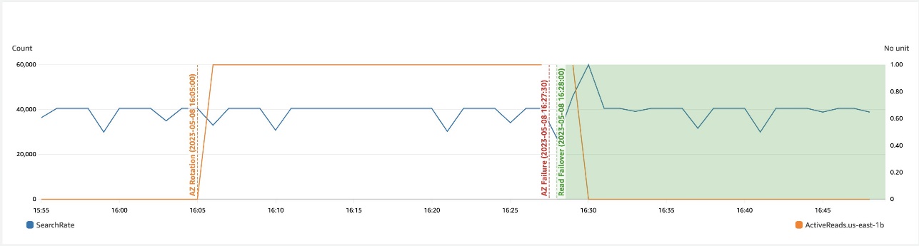
The following depicts that during a networking slowdown in a zone, write failover helps recover availability.

To ensure that the zonal failover mechanism is predictable (able to seamlessly shift traffic during an actual failure event), we regularly exercise failovers and keep rotating active and standby zones even during steady state. This not only verifies all network paths, ensuring we don’t hit surprises like clock skews, stale credentials, or networking issues during failover, but it also keeps gradually shifting caches to avoid cold starts on failovers, ensuring we deliver consistent performance at all times.
Improving the resiliency of the service
OpenSearch Service uses several principles and best practices to increase reliability, like automatic detection and faster recovery from failure, throttling excess requests, fail fast strategies, limiting queue sizes, quickly adapting to meet workload demands, implementing loosely coupled dependencies, continuously testing for failures, and more. We discuss a few of these methods in this section.
Automatic failure detection and recovery
All faults get monitored at a minutely granularity, across multiple sub-minutely metrics data points. Once detected, the system automatically triggers a recovery action on the impacted node. Although most classes of failures discussed so far in this post refer to binary failures where the failure is definitive, there is another kind of failure: non-binary failures, termed gray failures, whose manifestations are subtle and usually defy quick detection. Slow disk I/O is one example, which causes performance to be adversely impacted. The monitoring system detects anomalies in I/O wait times, latencies, and throughput, to detect and replace a node with slow I/O. Faster and effective detection and quick recovery is our best bet for a wide variety of infrastructure failures beyond our control.
Effective workload management in a dynamic environment
We’ve studied workload patterns that cause the system either to be overloaded with too many requests, maxing out CPU/memory, or a few rogue queries that can that either allocate huge chunks of memory or runaway queries that can exhaust multiple cores, either degrading the latencies of other critical requests or causing multiple nodes to fail due to the system’s resources running low. Some of the improvements in this direction are being done as a part of search backpressure initiatives, starting with tracking the request footprint at various checkpoints that prevents accommodating more requests and cancels the ones already running if they breach the resource limits for a sustained duration. To supplement backpressure in traffic shaping, we use admission control, which provides capabilities to reject a request at the entry point to avoid doing non-productive work (requests either time out or get cancelled) when the system is already run high on CPU and memory. Most of the workload management mechanisms have configurable knobs. No one size fits all workloads, therefore we use Auto-Tune to control them more granularly.
The cluster manager performs critical coordination tasks like metadata management and cluster formation, and orchestrates a few background operations like snapshot and shard placement. We added a task throttler to control the rate of dynamic mapping updates, snapshot tasks, and so on to prevent overwhelming it and to let critical operations run deterministically all the time. But what happens when there is no cluster manager in the cluster? The next section covers how we solved this.
Decoupling critical dependencies
In the event of cluster manager failure, searches continue as usual, but all write requests start to fail. We concluded that allowing writes in this state should still be safe as long as it doesn’t need to update the cluster metadata. This change further improves the write availability without compromising data consistency. Other service dependencies were evaluated to ensure downstream dependencies can scale as the cluster grows.
Failure mode testing
Although it’s hard to mimic all kinds of failures, we rely on AWS Fault Injection Simulator (AWS FIS) to inject common faults in the system like node failures, disk impairment, or network impairment. Testing with AWS FIS regularly in our pipelines helps us improve our detection, monitoring, and recovery times.
Contributing to open source
OpenSearch is an open-source, community-driven software. Most of the changes including the high availability design to support active and standby zones have been contributed to open source; in fact, we follow an open-source first development model. The fundamental primitive that enables zonal traffic shift and failover is based on a weighted traffic routing policy (active zones are assigned weights as 1 and standby zones are assigned weights as 0). Write failovers use the zonal decommission action, which evacuates all traffic from a given zone. Resiliency improvements for search backpressure and cluster manager task throttling are some of the ongoing efforts. If you’re excited to contribute to OpenSearch, open up a GitHub issue and let us know your thoughts.
Summary
Efforts to improve reliability is a never-ending cycle as we continue to learn and improve. With the Multi-AZ with Standby feature, OpenSearch Service has integrated best practices for cluster configuration, improved workload management, and achieved four 9s of availability and consistent performance. OpenSearch Service also raised the bar by continuously verifying availability with zonal traffic rotations and automated tests via AWS FIS.
We are excited to continue our efforts into improving the reliability and fault tolerance even further and to see what new and existing solutions builders can create using OpenSearch Service. We hope this leads to a deeper understanding of the right level of availability based on the needs of your business and how this offering achieves the availability SLA. We would love to hear from you, especially about your success stories achieving high levels of availability on AWS. If you have other questions, please leave a comment.
About the authors
 Bukhtawar Khan is a Principal Engineer working on Amazon OpenSearch Service. He is interested in building distributed and autonomous systems. He is a maintainer and an active contributor to OpenSearch.
 Gaurav Bafna is a Senior Software Engineer working on OpenSearch at Amazon Web Services. He is fascinated about solving problems in distributed systems. He is a maintainer and an active contributor to OpenSearch.
 Murali Krishna is a Senior Principal Engineer at AWS OpenSearch Service. He has built AWS OpenSearch Service and AWS CloudSearch. His areas of expertise include Information Retrieval, Large scale distributed computing, low latency real time serving systems etc. He has vast experience in designing and building web scale systems for crawling, processing, indexing and serving text and multimedia content. Prior to Amazon, he was part of Yahoo!, building crawling and indexing systems for their search products.
 Ranjith Ramachandra is a Senior Engineering Manager working on Amazon OpenSearch Service. He is passionate about highly scalable distributed systems, high performance and resilient systems.
Rohin Bhargava is a Sr. Product Manager with the Amazon OpenSearch Service team. His passion at AWS is to help customers find the correct mix of AWS services to achieve success for their business goals.
Amazon QuickSight is a scalable, serverless, machine learning (ML)-powered business intelligence (BI) solution that makes it easy to connect to your data, create interactive dashboards, get access to ML-enabled insights, and share visuals and dashboards with tens of thousands of internal and external users, either within QuickSight itself or embedded into any application.
A write-back is the ability to update a data mart, data warehouse, or any other database backend from within BI dashboards and analyze the updated data in near-real time within the dashboard itself. In this post, we show how to perform secure database write-backs with QuickSight.
Use case overview
To demonstrate how to enable a write-back capability with QuickSight, let’s consider a fictional company, AnyCompany Inc. AnyCompany is a professional services firm that specializes in providing workforce solutions to their customers. AnyCompany determined that running workloads in the cloud to support its growing global business needs is a competitive advantage and uses the cloud to host all its workloads. AnyCompany decided to enhance the way its branches provide quotes to its customers. Currently, the branches generate customer quotes manually, and as a first step in this innovation journey, AnyCompany is looking to develop an enterprise solution for customer quote generation with the capability to dynamically apply local pricing data at the time of quote generation.
AnyCompany currently uses Amazon Redshift as their enterprise data warehouse platform and QuickSight as their BI solution.
Building a new solution comes with the following challenges:
- AnyCompany wants a solution that is easy to build and maintain, and they don’t want to invest in building a separate user interface.
- AnyCompany wants to extend the capabilities of their existing QuickSight BI dashboard to also enable quote generation and quote acceptance. This will simplify feature rollouts because their employees already use QuickSight dashboards and enjoy the easy-to-use interface that QuickSight provides.
- AnyCompany wants to store the quote negotiation history that includes generated, reviewed, and accepted quotes.
- AnyCompany wants to build a new dashboard with quote history data for analysis and business insights.
This post goes through the steps to enable write-back functionality to Amazon Redshift from QuickSight. Note that the traditional BI tools are read-only with little to no options to update source data.
Solution overview
This solution uses the following AWS services:
- Amazon API Gateway – Hosts and secures the write-back REST API that will be invoked by QuickSight
- AWS Lambda – Runs the compute function required to generate the hash and a second function to securely perform the write-back
- Amazon QuickSight – Offers BI dashboards and quote generation capabilities
- Amazon Redshift – Stores quotes, prices, and other relevant datasets
- AWS Secrets Manager – Stores and manages keys to sign hashes (message digest)
Although this solution uses Amazon Redshift as the data store, a similar approach can be implemented with any database that supports creating user-defined functions (UDFs) that can invoke Lambda.
The following figure shows the workflow to perform write-backs from QuickSight.

The first step in the solution is to generate a hash or a message digest of the set of attributes in Amazon Redshift by invoking a Lambda function. This step prevents request tampering. To generate a hash, Amazon Redshift invokes a scalar Lambda UDF. The hashing mechanism used here is the popular BLAKE2 function (available in the Python library hashlib). To further secure the hash, keyed hashing is used, which is a faster and simpler alternative to hash-based message authentication code (HMAC). This key is generated and stored by Secrets Manager and should be accessible only to allowed applications. After the secure hash is generated, it’s returned to Amazon Redshift and combined in an Amazon Redshift view.
Writing the generated quote back to Amazon Redshift is performed by the write-back Lambda function, and an API Gateway REST API endpoint is created to secure and pass requests to the write-back function. The write-back function performs the following actions:
- Generate the hash based on the API input parameters received from QuickSight.
- Sign the hash by applying the key from Secrets Manager.
- Compare the generated hash with the hash received from the input parameters using the compare\_digest method available in the HMAC module.
- Upon successful validation, write the record to the quote submission table in Amazon Redshift.
The following section provide detailed steps with sample payloads and code snippets.
Generate the hash
The hash is generated using a Lambda UDF in Amazon Redshift. Additionally, a Secrets Manager key is used to sign the hash. To create the hash, complete the following steps:
- Create the Secrets Manager key from the AWS Command Line Interface (AWS CLI):
- Create a Lambda UDF to generate a hash for encryption:
- Define an Amazon Redshift UDF to call the Lambda function to create a hash:
The AWS Identity and Access Management (IAM) role in the preceding step should have the following policy attached to be able to invoke the Lambda function:
- Fetch the key from Secrets Manager.
This key is used by the Lambda function to further secure the hash. This is indicated in the get\_secret function in Step 2.
Set up Amazon Redshift datasets in QuickSight
The quote generation dashboard uses the following Amazon Redshift view.

Create an Amazon Redshift view that uses all the preceding columns along with the hash column:
The records will look like the following screenshot.

The preceding view will be used as the QuickSight dataset to generate quotes. A QuickSight analysis will be created using the dataset. For near-real-time analysis, you can use QuickSight direct query mode.
Create API Gateway resources
The write-back operation is initiated by QuickSight invoking an API Gateway resource, which invokes the Lambda write-back function. As a prerequisite for creating the calculated field in QuickSight to call the write-back API, you must first create these resources.
API Gateway secures and invokes the write-back Lambda function with the parameters created as URL query string parameters with mapping templates. The mapping parameters can be avoided by using the Lambda proxy integration.
Create a REST API resource of method type GET that uses Lambda functions (created in the next step) as the integration type. For instructions, refer to Creating a REST API in Amazon API Gateway and Set up Lambda integrations in API Gateway.
The following screenshot shows the details for creating a query string parameter for each parameter passed to API Gateway.

The following screenshot shows the details for creating a mapping template parameter for each parameter passed to API Gateway.

Create the Lambda function
Create a new Lambda function for the API Gateway to invoke. The Lambda function performs the following steps:
- Receive parameters from QuickSight through API Gateway and hash the concatenated parameters.
The following code example retrieves parameters from the API Gateway call using the event object of the Lambda function:
The function performs the hashing logic as shown in the create hash step earlier using the concatenated parameters passed by QuickSight.
- Compare the hashed output with the hash parameter.
If these don’t match, the write-back won’t happen.
- If the hashes match, perform a write-back. Check for the presence of a record in the quote generation table by generating a query from the table using the parameters passed from QuickSight:
- Complete the following action based on the results of the query:
- If no record exists for the preceding combination, generate and run an insert query using all parameters with the status as generated.
- If a record exists for the preceding combination, generate and run an insert query with the status as in review. The quote\_Id for the existing combination will be reused.
Create a QuickSight visual
This step involves creating a table visual that uses a calculated field to pass parameters to API Gateway and invoke the preceding Lambda function.
- Add a QuickSight calculated field named Generate Quote to hold the API Gateway hosted URL that will be triggered to write back the quote history into Amazon Redshift:
- Create a QuickSight table visual.
- Add required fields such as Customer, Skill, and Cost.
- Add the Generate Quote calculated field and style this as a hyperlink.
Choosing this link will write the record into Amazon Redshift. This is incumbent on the same hash value returning when the Lambda function performs the hash on the parameters.

The following screenshot shows a sample table visual.

Write to the Amazon Redshift database
The Secrets Manager key is fetched and used by the Lambda function to generate the hash for comparison. The write-back will be performed only if the hash matches with the hash passed in the parameter.
The following Amazon Redshift table will capture the quote history as populated by the Lambda function. Records in green represent the most recent records for the quote.

Considerations and next steps
Using secure hashes prevents the tampering of payload parameters that are visible in the browser window when the write-back URL is invoked. To further secure the write-back URL, you can employ the following techniques:
- Deploy the REST API in a private VPC that is accessible only to QuickSight users.
- To prevent replay attacks, a timestamp can be generated alongside the hashing function and passed as an additional parameter in the write-back URL. The backend Lambda function can then be modified to only allow write-backs within a certain time-based threshold.
- Follow the API Gateway access control and security best practices.
- Mitigate potential Denial of Service for public-facing APIs.
You can further enhance this solution to render a web-based form when the write-back URL is opened. This could be implemented by dynamically generating an HTML form in the backend Lambda function to support the input of additional information. If your workload requires a high number of write-backs that require higher throughput or concurrency, a purpose-built data store like Amazon Aurora PostgreSQL-Compatible Edition might be a better choice. For more information, refer to Invoking an AWS Lambda function from an Aurora PostgreSQL DB cluster. These updates can then be synchronized into Amazon Redshift tables using federated queries.
Conclusion
This post showed how to use QuickSight along with Lambda, API Gateway, Secrets Manager, and Amazon Redshift to capture user input data and securely update your Amazon Redshift data warehouse without leaving your QuickSight BI environment. This solution eliminates the need to create an external application or user interface for database update or insert operations, and reduces related development and maintenance overhead. The API Gateway call can also be secured using a key or token to ensure only calls originating from QuickSight are accepted by the API Gateway. This will be covered in subsequent posts.
About the Authors
Srikanth Baheti is a Specialized World Wide Principal Solutions Architect for Amazon QuickSight. He started his career as a consultant and worked for multiple private and government organizations. Later he worked for PerkinElmer Health and Sciences & eResearch Technology Inc, where he was responsible for designing and developing high traffic web applications, highly scalable and maintainable data pipelines for reporting platforms using AWS services and Serverless computing.
Raji Sivasubramaniam is a Sr. Solutions Architect at AWS, focusing on Analytics. Raji is specialized in architecting end-to-end Enterprise Data Management, Business Intelligence and Analytics solutions for Fortune 500 and Fortune 100 companies across the globe. She has in-depth experience in integrated healthcare data and analytics with wide variety of healthcare datasets including managed market, physician targeting and patient analytics.
 Vaidy Janardhanam is a Data Lab Architect at AWS, focusing on Analytics. Vaidy works with AWS customers to help them design and build data and analytics applications in the cloud. He has accelerated the path to production for customers across the globe using AWS services like QuickSight, Redshift, Lambda.
 Ranjit Rajan is a Principal Data Lab Solutions Architect with AWS. Ranjit works with AWS customers to help them design and build data and analytics applications in the cloud.
AWS Glue Studio is a graphical interface that makes it easy to create, run, and monitor extract, transform, and load (ETL) jobs in AWS Glue. It allows you to visually compose data transformation workflows using nodes that represent different data handling steps, which later are converted automatically into code to run.
AWS Glue Studio recently released 10 more visual transforms to allow creating more advanced jobs in a visual way without coding skills. In this post, we discuss potential uses cases that reflect common ETL needs.
The new transforms that will be demonstrated in this post are: Concatenate, Split String, Array To Columns, Add Current Timestamp, Pivot Rows To Columns, Unpivot Columns To Rows, Lookup, Explode Array Or Map Into Columns, Derived Column, and Autobalance Processing.
Solution overview
In this use case, we have some JSON files with stock option operations. We want to make some transformations before storing the data to make it easier to analyze, and we also want to produce a separate dataset summary.
In this dataset, each row represents a trade of option contracts. Options are financial instruments that provide the right—but not the obligation—to buy or sell stock shares at a fixed price (called strike price) before a defined expiration date.
Input data
The data follows the following schema:
- order\_id – A unique ID
- symbol – A code generally based on a few letters to identify the corporation that emits the underlying stock shares
- instrument – The name that identifies the specific option being bought or sold
- currency – The ISO currency code in which the price is expressed
- price – The amount that was paid for the purchase of each option contract (on most exchanges, one contract allows you to buy or sell 100 stock shares)
- exchange – The code of the exchange center or venue where the option was traded
- sold – A list of the number of contracts that where allocated to fill the sell order when this is a sell trade
- bought – A list of the number of contracts that where allocated to fill the buy order when this is buy trade
The following is a sample of the synthetic data generated for this post:
ETL requirements
This data has a number of unique characteristics, as often found on older systems, that make the data harder to use.
The following are the ETL requirements:
- The instrument name has valuable information that is intended for humans to understand; we want to normalize it into separate columns for easier analysis.
- The attributes
boughtandsoldare mutually exclusive; we can consolidate them into a single column with the contract numbers and have another column indicating if the contracts where bought or sold in this order. - We want to keep the information about the individual contract allocations but as individual rows instead of forcing users to deal with an array of numbers. We could add up the numbers, but we would lose information about how the order was filled (indicating market liquidity). Instead, we choose to denormalize the table so each row has a single number of contracts, splitting orders with multiple numbers into separate rows. In a compressed columnar format, the extra dataset size of this repetition is often small when compression is applied, so it’s acceptable to make the dataset easier to query.
- We want to generate a summary table of volume for each option type (call and put) for each stock. This provides an indication of the market sentiment for each stock and the market in general (greed vs. fear).
- To enable overall trade summaries, we want to provide for each operation the grand total and standardize the currency to US dollars, using an approximate conversion reference.
- We want to add the date when these transformations took place. This could be useful, for instance, to have a reference on when was the currency conversion made.
Based on those requirements, the job will produce two outputs:
- A CSV file with a summary of the number of contracts for each symbol and type
- A catalog table to keep a history of the order, after doing the transformations indicated

Prerequisites
You will need your own S3 bucket to follow along with this use case. To create a new bucket, refer to Creating a bucket.
Generate synthetic data
To follow along with this post (or experiment with this kind of data on your own), you can generate this dataset synthetically. The following Python script can be run on a Python environment with Boto3 installed and access to Amazon Simple Storage Service (Amazon S3).
To generate the data, complete the following steps:
- On AWS Glue Studio, create a new job with the option Python shell script editor.
- Give the job a name and on the Job details tab, select a suitable role and a name for the Python script.
- In the Job details section, expand Advanced properties and scroll down to Job parameters.
- Enter a parameter named
--bucketand assign as the value the name of the bucket you want to use to store the sample data. - Enter the following script into the AWS Glue shell editor:
- Run the job and wait until it shows as successfully completed on the Runs tab (it should take just a few seconds).
Each run will generate a JSON file with 1,000 rows under the bucket specified and prefix transformsblog/inputdata/. You can run the job multiple times if you want to test with more input files.
Each line in the synthetic data is a data row representing a JSON object like the following:
Create the AWS Glue visual job
To create the AWS Glue visual job, complete the following steps:
- Go to AWS Glue Studio and create a job using the option Visual with a blank canvas.
- Edit
Untitled jobto give it a name and assign a role suitable for AWS Glue on the Job details tab. - Add an S3 data source (you can name it
JSON files source) and enter the S3 URL under which the files are stored (for example,s3://<your bucket name>/transformsblog/inputdata/), then select JSON as the data format. - Select Infer schema so it sets the output schema based on the data.
From this source node, you’ll keep chaining transforms. When adding each transform, make sure the selected node is the last one added so it gets assigned as the parent, unless indicated otherwise in the instructions.
If you didn’t select the right parent, you can always edit the parent by selecting it and choosing another parent in the configuration pane.

For each node added, you’ll give it a specific name (so the node purpose shows in the graph) and configuration on the Transform tab.
Every time a transform changes the schema (for instance, add a new column), the output schema needs to be updated so it’s visible to the downstream transforms. You can manually edit the output schema, but it’s more practical and safer to do it using the data preview.
Additionally, that way you can verify the transformation are working so far as expected. To do so, open the Data preview tab with the transform selected and start a preview session. After you have verified the transformed data looks as expected, go to the Output schema tab and choose Use data preview schema to update the schema automatically.
As you add new kinds of transforms, the preview might show a message about a missing dependency. When this happens, choose End Session and the start a new one, so the preview picks up the new kind of node.
Extract instrument information
Let’s start by dealing with the information on the instrument name to normalize it into columns that are easier to access in the resulting output table.
- Add a Split String node and name it
Split instrument, which will tokenize the instrument column using a whitespace regex:\s+(a single space would do in this case, but this way is more flexible and visually clearer). - We want to keep the original instrument information as is, so enter a new column name for the split array:
instrument\_arr.

- Add an Array To Columns node and name it
Instrument columnsto convert the array column just created into new fields, except forsymbol, for which we already have a column. - Select the column
instrument\_arr, skip the first token and tell it to extract the output columnsmonth, day, year, strike\_price, typeusing indexes2, 3, 4, 5, 6(the spaces after the commas are for readability, they don’t impact the configuration).

The year extracted is expressed with two digits only; let’s put a stopgap to assume it’s in this century if they just use two digits.
- Add a Derived Column node and name it
Four digits year. - Enter
yearas the derived column so it overrides it, and enter the following SQL expression:
CASE WHEN length(year) = 2 THEN ('20' || year) ELSE year END

For convenience, we build an expiration\_date field that a user can have as reference of the last date the option can be exercised.
- Add a Concatenate Columns node and name it
Build expiration date. - Name the new column
expiration\_date, select the columnsyear,month, andday(in that order), and a hyphen as spacer.

The diagram so far should look like the following example.

The data preview of the new columns so far should look like the following screenshot.

Normalize the number of contracts
Each of the rows in the data indicates the number of contracts of each option that were bought or sold and the batches on which the orders were filled. Without losing the information about the individual batches, we want to have each amount on an individual row with a single amount value, while the rest of the information is replicated in each row produced.
First, let’s merge the amounts into a single column.
- Add an Unpivot Columns Into Rows node and name it
Unpivot actions. - Choose the columns
boughtandsoldto unpivot and store the names and values in columns namedactionandcontracts, respectively.

Notice in the preview that the new columncontractsis still an array of numbers after this transformation.
- Add an Explode Array Or Map into Rows row named
Explode contracts. - Choose the
contractscolumn and entercontractsas the new column to override it (we don’t need to keep the original array).
The preview now shows that each row has a single contracts amount, and the rest of the fields are the same.
This also means that order\_id is no longer a unique key. For your own use cases, you need to decide how to model your data and if you want to denormalize or not.

The following screenshot is an example of what the new columns look like after the transformations so far.

Create a summary table
Now you create a summary table with the number of contracts traded for each type and each stock symbol.
Let’s assume for illustration purposes that the files processed belong to a single day, so this summary gives the business users information about what the market interest and sentiment are that day.
- Add a Select Fields node and select the following columns to keep for the summary:
symbol,type, andcontracts.

- Add a Pivot Rows Into Columns node and name it
Pivot summary. - Aggregate on the
contractscolumn usingsumand choose to convert thetypecolumn.

Normally, you would store it on some external database or file for reference; in this example, we save it as a CSV file on Amazon S3.
- Add an Autobalance Processing node and name it
Single output file. - Although that transform type is normally used to optimize the parallelism, here we use it to reduce the output to a single file. Therefore, enter
1in the number of partitions configuration.

- Add an S3 target and name it
CSV Contract summary. - Choose CSV as the data format and enter an S3 path where the job role is allowed to store files.
The last part of the job should now look like the following example.

- Save and run the job. Use the Runs tab to check when it has finished successfully.
You’ll find a file under that path that is a CSV, despite not having that extension. You’ll probably need to add the extension after downloading it to open it.
On a tool that can read the CSV, the summary should look something like the following example.

Clean up temporary columns
In preparation for saving the orders into a historical table for future analysis, let’s clean up some temporary columns created along the way.
- Add a Drop Fields node with the
Explode contractsnode selected as its parent (we are branching the data pipeline to generate a separate output). - Select the fields to be dropped:
instrument\_arr,month,day, andyear.
The rest we want to keep so they are saved in the historical table we’ll create later.

Currency standardization
This synthetic data contains fictional operations on two currencies, but in a real system you could get currencies from markets all over the world. It’s useful to standardize the currencies handled into a single reference currency so they can be easily be compared and aggregated for reporting and analysis.
We use Amazon Athena to simulate a table with approximate currency conversions that gets updated periodically (here we assume we process the orders timely enough that the conversion is a reasonable representative for comparison purposes).
- Open the Athena console in the same Region where you’re using AWS Glue.
- Run the following query to create the table by setting an S3 location where both your Athena and AWS Glue roles can read and write. Also, you might want to store the table in a different database than
default(if you do that, update the table qualified name accordingly in the examples provided). - Enter a few sample conversions into the table:
INSERT INTO default.exchange\_rates VALUES ('usd', 1.0), ('eur', 1.09), ('gbp', 1.24); - You should now be able to view the table with the following query:
SELECT * FROM default.exchange\_rates

- Back on the AWS Glue visual job, add a Lookup node (as a child of
Drop Fields) and name itExchange rate. - Enter the qualitied name of the table you just created, using
currencyas the key and select theexchange\_ratefield to use.
Because the field is named the same in both the data and the lookup table, we can just enter the namecurrencyand don’t need to define a mapping.
At the time of this writing, the Lookup transform is not supported in the data preview and it will show an error that the table doesn’t exist. This is only for the data preview and doesn’t prevent the job from running correctly. The few remaining steps of the post don’t require you to update the schema. If you need to run a data preview on other nodes, you can remove the lookup node temporarily and then put it back. - Add a Derived Column node and name it
Total in usd. - Name the derived column
total\_usdand use the following SQL expression:
round(contracts * price * exchange\_rate, 2)

- Add a Add Current Timestamp node and name the column
ingest\_date. - Use the format
%Y-%m-%dfor your timestamp (for demonstration purposes, we are just using the date; you can make it more precise if you want to).

Save the historical orders table
To save the historical orders table, complete the following steps:
- Add an S3 target node and name it
Orders table. - Configure Parquet format with snappy compression, and provide an S3 target path under which to store the results (separate from the summary).
- Select Create a table in the Data Catalog and on subsequent runs, update the schema and add new partitions.
- Enter a target database and a name for the new table, for instance:
option\_orders.

The last part of the diagram should now look similar to the following, with two branches for the two separate outputs.

After you run the job successfully, you can use a tool like Athena to review the data the job has produced by querying the new table. You can find the table on the Athena list and choose Preview table or just run a SELECT query (updating the table name to the name and catalog you used):
SELECT * FROM default.option\_orders limit 10
Your table content should look similar to the following screenshot.

Clean up
If you don’t want to keep this example, delete the two jobs you created, the two tables in Athena, and the S3 paths where the input and output files were stored.
Conclusion
In this post, we showed how the new transforms in AWS Glue Studio can help you do more advanced transformation with minimum configuration. This means you can implement more ETL uses cases without having to write and maintain any code. The new transforms are already available on AWS Glue Studio, so you can use the new transforms today in your visual jobs.
About the author
 Gonzalo Herreros is a Senior Big Data Architect on the AWS Glue team.
Customers of Amazon OpenSearch Service can already use Security Assertion Markup Language (SAML) to access OpenSearch Dashboards.
This post outlines two methods by which programmatic users can now access OpenSearch using SAML identities. This applies to all identity providers (IdPs) that support SAML 2.0, including prevalent ones like Active Directory Federation Service (ADFS), Okta, AWS IAM Identity Center (Successor to AWS Single Sign-On), KeyCloak, and others. Although we outline the methods as they pertain to OpenSearch Service and AWS Identity and Access Management (IAM), programmatic access to each of these individual providers is outside the scope of this post. Most of these providers do provide such a facility.
Single sign-on methods
When you use single sign-on (SSO), there are two different authentication methods:
- Identity provider initiated – This is when a user or a user-agent first authenticates with an IdP and gets a SAML assertion that establishes the identity of the user. This assertion is then passed to a service provider (SP) that provides access to a protected resource.
- Service provider initiated – Although the IdP-initiated exchange is straightforward, a more typical sign-on experience is when the protected resource is accessed directly. The SP then redirects the user to the IdP for authentication along with a SAML authentication request. The IdP responds with an authentication assertion inside a SAML response. After that, the SSO experience is the same as that of an IdP-initiated flow.
For programmatic access to OpenSearch Service, an external IdP is the IdP, and OpenSearch Service and IAM both serve as SPs. To configure your IdP of choice as the SAML IdP for IAM, refer to Creating IAM SAML identity providers. To configure OpenSearch Service, refer to SAML authentication for OpenSearch Dashboards.
In the following sections, we outline two methods to access OpenSearch Service API:
- Using AWS Security Token Service (AWS STS)
- Using the OpenSearch Dashboards’ console proxy
Method 1: Use AWS STS
The following figure shows the sequence of calls to access OpenSearch Service API using AWS STS.
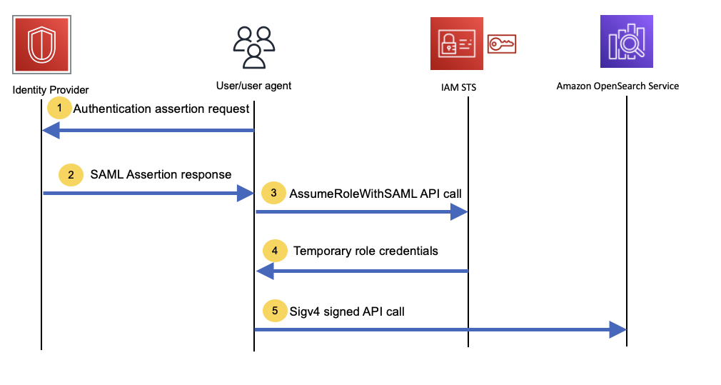
Let’s explore each step in more detail.
Steps 1 and 2
Steps 1 and 2 vary depending upon your chosen IdP. In general, they typically provide an authentication API or session API or another similar API to authenticate and retrieve the SAML authentication assertion response. We use this SAML assertion in the next step.
Steps 3 and 4
Call the AssumeRoleWithSAML AWS STS API to exchange the SAML assertion for temporary credentials associated with your SAML identity. See the following code:
Step 5
Use the temporary credentials from the last step to sign all API requests to OpenSearch Service. Also ensure the role that you assumed with the AssumeRoleWithSAML call has sufficient permission to access the requisite data in OpenSearch Service. Refer to Mapping roles to users for more information about mapping this role as a backend role. As an additional step to ensure consistency, this AWS STS role and any SAML group the user is part of can be mapped to the same role in OpenSearch Service. The following code shows a model to make this call:
Method 2: Use OpenSearch Dashboards’ console proxy
OpenSearch Dashboards has a component called a console proxy that can proxy requests to OpenSearch. This allows OpenSearch clients to make the same API calls in Domain Specific Language (DSL) to this console proxy instead of directly calling OpenSearch. The console proxy forwards these calls to OpenSearch and responds back to the clients in the same format as OpenSearch.
The following figure shows the sequence of calls you can make to the console proxy to gain programmatic access to OpenSearch Service.
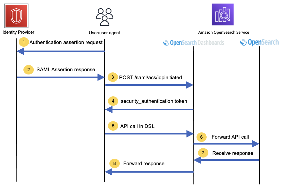
Steps 1 and 2
The first two steps are similar to method 1, and they will vary depending on what IdP is chosen. Essentially, you need to obtain a SAML authentication assertion response from the IdP.
Steps 3 and 4
Use the SAML assertion from the previous steps and POST it to the Assertion Consumer Service (ACS) URL, \_opendistro/\_security/saml/acs/idpinitiated, to exchange the assertion for the security\_authentication token. The following code shows the command line for these steps:
If you’re using the OpenSearch engine, the dashboard URL is <domain URL>/\_dashboards. If you’re using the Elasticsearch engine, the dashboard URL is <domain URL>/\_plugin/kibana. OpenSearch Dashboards processes this and responds with a redirect response with code 302 and an empty body. The response headers now also contain a cookie named security\_authentication, which is the token you must use in all subsequent calls.
Steps 5–8
Use the security\_authentication cookie in the API calls to the console proxy to perform programmatic API calls. The following code shows a command line for these steps:
Make sure to include a header called osd-xsrf : true for programmatic access to dashboards. The console proxy path is /api/console/proxy for Elasticsearch engines version 6.x and 7.x and OpenSearch engine version 1.x and 2.x.
Similar to method 1, make sure to map roles and groups associated with a particular SAML identity as the correct backend role with requisite permissions.
Comparing these methods
You can use method 1 in any domain regardless of the engine as long as fine-grained access control is enabled. Method 2 only works for domains with Elasticsearch engine versions greater than 6.7 and all OpenSearch engine versions.
The OpenSearch Dashboards process is generally meant for human interactions, which has a lower API call rate and volume than those of programmatic calls. OpenSearch can handle considerably higher API call rates and volume, so take care not to send high-volume API calls using method 2. As a best practice for programmatic access with SAML identities, we recommend method 1 wherever possible to avoid performance bottlenecks.
Conclusion
Both of the methods outlined in this post provide a similar flow to access OpenSearch Service programmatically using SAML identities (exchanging a SAML assertion for an authentication token). AssumeRoleWithSAML is a key and fairly straightforward-to-use API that enables this access and is our recommended method. Try one of OpenSearch Service labs and launch an OpenSearch Service domain to experiment with these methods. Good luck!
About the author
 Muthu Pitchaimani is a Search Specialist with Amazon OpenSearch Service. He builds large-scale search applications and solutions. Muthu is interested in the topics of networking and security, and is based out of Austin, Texas.
Hundreds of thousands of customers use AWS Glue, a serverless data integration service, to discover, prepare, and combine data for analytics, machine learning (ML), and application development. AWS Glue for Apache Spark jobs work with your code and configuration of the number of data processing units (DPU). Each DPU provides 4 vCPU, 16 GB memory, and 64 GB disk. AWS Glue manages running Spark and adjusts workers to achieve the best price performance. For workloads such as data transforms, joins, and queries, you can use G.1X (1 DPU) and G.2X (2 DPU) workers, which offer a scalable and cost-effective way to run most jobs. With exponentially growing data sources and data lakes, customers want to run more data integration workloads, including their most demanding transforms, aggregations, joins, and queries. These workloads require higher compute, memory, and storage per worker.
Today we are pleased to announce the general availability of AWS Glue G.4X (4 DPU) and G.8X (8 DPU) workers, the next series of AWS Glue workers for the most demanding data integration workloads. G.4X and G.8X workers offer increased compute, memory, and storage, making it possible for you to vertically scale and run intensive data integration jobs, such as memory-intensive data transforms, skewed aggregations, and entity detection checks involving petabytes of data. Larger worker types not only benefit the Spark executors, but also in cases where the Spark driver needs larger capacity—for instance, because the job query plan is quite large.
This post demonstrates how AWS Glue G.4X and G.8X workers help you scale your AWS Glue for Apache Spark jobs.
G.4X and G.8X workers
AWS Glue G.4X and G.8X workers give you more compute, memory, and storage to run your most demanding jobs. G.4X workers provide 4 DPU, with 16 vCPU, 64 GB memory, and 256 GB of disk per node. G.8X workers provide 8 DPU, with 32 vCPU, 128 GB memory, and 512 GB of disk per node. You can enable G.4X and G.8X workers with a single parameter change in the API, AWS Command Line Interface (AWS CLI), or visually in AWS Glue Studio. Regardless of the worker used, all AWS Glue jobs have the same capabilities, including auto scaling and interactive job authoring via notebooks. G.4X and G.8X workers are available with AWS Glue 3.0 and 4.0.
The following table shows compute, memory, disk, and Spark configurations per worker type in AWS Glue 3.0 or later.
| AWS Glue Worker Type | DPU per Node | vCPU | Memory (GB) | Disk (GB) | Number of Spark Executors per Node | Number of Cores per Spark Executor |
| G.1X | 1 | 4 | 16 | 64 | 1 | 4 |
| G.2X | 2 | 8 | 32 | 128 | 1 | 8 |
| G.4X (new) | 4 | 16 | 64 | 256 | 1 | 16 |
| G.8X (new) | 8 | 32 | 128 | 512 | 1 | 32 |
To use G.4X and G.8X workers on an AWS Glue job, change the setting of the worker type parameter to G.4X or G.8X. In AWS Glue Studio, you can choose G 4X or G 8X under Worker type.

In the AWS API or AWS SDK, you can specify G.4X or G.8X in the WorkerType parameter. In the AWS CLI, you can use the --worker-type parameter in a create-job command.
To use G.4X and G.8X on an AWS Glue Studio notebook or interactive sessions, set G.4X or G.8X in the %worker\_type magic:

Performance characteristics using the TPC-DS benchmark
In this section, we use the TPC-DS benchmark to showcase performance characteristics of the new G.4X and G.8X worker types. We used AWS Glue version 4.0 jobs.
G.2X, G.4X, and G.8X results with the same number of workers
Compared to the G.2X worker type, the G.4X worker has 2 times the DPUs and the G.8X worker has 4 times the DPUs. We ran over 100 TPC-DS queries against the 3 TB TPC-DS dataset with the same number of workers but on different worker types. The following table shows the results of the benchmark.
| Worker Type | Number of Workers | Number of DPUs | Duration (minutes) | Cost at $0.44/DPU-hour ($) |
| G.2X | 30 | 60 | 537.4 | $236.46 |
| G.4X | 30 | 120 | 264.6 | $232.85 |
| G.8X | 30 | 240 | 122.6 | $215.78 |

When running jobs on the same number of workers, the new G.4X and G.8x workers achieved roughly linear vertical scalability.
G.2X, G.4X, and G.8X results with the same number of DPUs
We ran over 100 TPC-DS queries against the 10 TB TPC-DS dataset with the same number of DPUs but on different worker types. The following table shows the results of the experiments.
| Worker Type | Number of Workers | Number of DPUs | Duration (minutes) | Cost at $0.44/DPU-hour ($) |
| G.2X | 40 | 80 | 1323 | $776.16 |
| G.4X | 20 | 80 | 1191 | $698.72 |
| G.8X | 10 | 80 | 1190 | $698.13 |

When running jobs on the same number of total DPUs, the job performance stayed mostly the same with new worker types.
Example: Memory-intensive transformations
Data transformations are an essential step to preprocess and structure your data into an optimal form. Bigger memory footprints are consumed in some transformations such as aggregation, join, your own custom logic using user-defined functions (UDFs), and so on. The new G.4X and G.8X workers enable you to run larger memory-intensive transformations at scale.
The following example reads large JSON files compressed in GZIP from an input Amazon Simple Storage Service (Amazon S3) location, performs groupBy, calculates groups based on K-means clustering using a Pandas UDF, then shows the results. Note that this UDF-based K-means is used just for illustration purposes; it’s recommended to use native K-means clustering for production purposes.
With G.2X workers
When an AWS Glue job runs on 12 G.2X workers (24 DPU), it failed due to a No space left on device error. On the Spark UI, the Stages tab for the failed stage shows that there were multiple failed tasks in the AWS Glue job due to the error.

The Executor tab shows failed tasks per executor.

Generally, G.2X workers can process memory-intensive workload well. This time, we used a special Pandas UDF that consumes a significant amount of memory, and it caused a failure due to a large amount of shuffle writes.
With G.8X workers
When an AWS Glue job runs on 3 G.8X workers (24 DPU), it succeeded without any failures, as shown on the Spark UI’s Jobs tab.

The Executors tab also explains that there were no failed tasks.

From this result, we observed that G.8X workers processed the same workload without failures.
Conclusion
In this post, we demonstrated how AWS Glue G.4X and G.8X workers can help you vertically scale your AWS Glue for Apache Spark jobs. G.4X and G.8X workers are available today in US East (Ohio), US East (N. Virginia), US West (Oregon), Asia Pacific (Singapore), Asia Pacific (Sydney), Asia Pacific (Tokyo), Canada (Central), Europe (Frankfurt), Europe (Ireland), and Europe (Stockholm). You can start using the new G.4X and G.8X worker types to scale your workload from today. To get started with AWS Glue, visit AWS Glue.
About the authors
Noritaka Sekiyama is a Principal Big Data Architect on the AWS Glue team. He works based in Tokyo, Japan. He is responsible for building software artifacts to help customers. In his spare time, he enjoys cycling with his road bike.
 Tomohiro Tanaka is a Senior Cloud Support Engineer on the AWS Support team. He’s passionate about helping customers build data lakes using ETL workloads. In his free time, he enjoys coffee breaks with his colleagues and making coffee at home.
 Chuhan Liu is a Software Development Engineer on the AWS Glue team. He is passionate about building scalable distributed systems for big data processing, analytics, and management. In his spare time, he enjoys playing tennis.
 Matt Su is a Senior Product Manager on the AWS Glue team. He enjoys helping customers uncover insights and make better decisions using their data with AWS Analytic services. In his spare time, he enjoys skiing and gardening.
Are you looking to understand the relationships between two numerical variables? Scatter plots are a powerful visual type that allow you to identify patterns, outliers, and strength of relationships between variables. In this post, we walk you through the newly launched scatter plot features in Amazon QuickSight, which will help you take your correlation analysis to the next level.
Feature overview
The scatter plot is undoubtedly one of the most effective visualizations for correlation analysis, helping to identify patterns, outliers, and the strength of the relationship between two or three variables (using a bubble chart). We have improved the performance and versatility of our scatter plots, supporting five additional use cases. The following functionalities have been added in this release:
- Display unaggregated values – Previously, when there was no field placed on Color, QuickSight displayed unaggregated values, and when a field was placed on Color, the metrics would be aggregated and grouped by that dimension. Now, you can choose to plot unaggregated values even if you’re using a field on Color by using the new aggregate option called None from the field menu, in addition to aggregation options like Sum, Min, and Max. If one value is set to be aggregated, the other value will be automatically set as aggregated, and the same applies to unaggregated scenarios. Mixed aggregation scenarios are not supported, meaning that one value can’t be set as aggregated while the other is unaggregated. It’s worth noting that the unaggregated scenario (the None option) is only supported for numerical values, whereas categorical values (like dates and dimensions) will only display aggregate values such as Count and Count distinct.

- Support for an additional Label field – We’re introducing a new field well called Label alongside the existing Color field. This will allow you to color by one field and label by another, providing more flexibility in data visualization.

- Faster load time – The load time is up to six times faster, which impacts both new and existing use cases. Upon launch, you’ll notice that scatter plots render noticeably faster, especially when dealing with larger datasets.
Explore advanced scatter plot use cases
You can choose to set both X and Y values to either aggregated or unaggregated (the None option) from the X and Y axis field menus. This will define if values will be aggregated by dimensions in the Color and Label field wells or not. To get started, add the required fields and choose the appropriate aggregation based on your use case.
Unaggregated use cases
The following screenshot shows an example of unaggregated X and Y value with Color.

The following screenshot shows an example of unaggregated X and Y with Label.

The following screenshot shows an example of unaggregated X and Y with Color and Label.

Aggregated use cases
The following screenshot shows an example of X and Y aggregated by Color.

The following screenshot shows an example of X and Y aggregated by Label.

The following screenshot shows an example of X and Y aggregated by Color and Label.

Conclusion
In summary, our enhanced scatter plots offer users greater performance and versatility, catering to a wider range of use cases than before. The ability to display unaggregated values and support for additional label fields gives users the flexibility they need to visualize the data they want. For further details, refer to Amazon QuickSight Scatterplot. Try out the new scatter plot updates and let us know your feedback in the comments section.
About the authors
 Bhupinder Chadha is a senior product manager for Amazon QuickSight focused on visualization and front end experiences. He is passionate about BI, data visualization and low-code/no-code experiences. Prior to QuickSight he was the lead product manager for Inforiver, responsible for building a enterprise BI product from ground up. Bhupinder started his career in presales, followed by a small gig in consulting and then PM for xViz, an add on visualization product.
Amazon Redshift Serverless makes it easy to run and scale analytics in seconds without the need to set up and manage data warehouse clusters. With Redshift Serverless, users such as data analysts, developers, business professionals, and data scientists can get insights from data by simply loading and querying data in the data warehouse.
Customers use their preferred SQL clients to analyze their data in Redshift Serverless. They want to use an identity provider (IdP) or single sign-on (SSO) credentials to connect to Redshift Serverless to reuse existing using credentials and avoid additional user setup and configuration. When you use AWS Identity and Access Management (IAM) or IdP-based credentials to connect to a serverless data warehouse, Amazon Redshift automatically creates a database user for the end-user. You can simplify managing user privileges by using role-based access control. Admins can use a database-role mapping for SSO with the IAM roles that users are assigned to get their database privileges automatically. With this integration, organizations can simplify user management because they no longer need to create users and map them to database roles manually. You can define the mapped database roles as a principal tag for the IdP groups or IAM role, so Amazon Redshift database roles and users who are members of those IdP groups are granted to the database roles automatically.
In this post, we focus on Okta as the IdP and provide step-by-step guidance to integrate Redshift Serverless with Okta using the Amazon Redshift Query Editor V2 and with SQL clients like SQL Workbench/J. You can use this mechanism with other IdP providers such as Azure Active Directory or Ping with any applications or tools using Amazon’s JDBC/ODBC/Python driver.
Solution overview
The following diagram illustrates the authentication flow of Okta with Redshift Serverless using federated IAM roles and automatic database-role mapping.

The workflow contains the following steps:
- Either the user chooses an IdP app in their browser, or the SQL client initiates a user authentication request to the IdP (Okta).
- Upon a successful authentication, Okta submits a request to the AWS federation endpoint with a SAML assertion containing the PrincipalTags.
- The AWS federation endpoint validates the SAML assertion and invokes the AWS Security Token Service (AWS STS) API AssumeRoleWithSAML. The SAML assertion contains the IdP user and group information that is stored in the RedshiftDbUser and RedshiftDbRoles principal tags, respectively. Temporary IAM credentials are returned to the SQL client or, if using the Query Editor v2, the user’s browser is redirected to the Query Editor v2 console using the temporary IAM credentials.
- The temporary IAM credentials are used by the SQL client or Query Editor v2 to call the Redshift Serverless GetCredentials API. The API uses the principal tags to determine the user and database roles that the user belongs to. An associated database user is created if the user is signing in for the first time and is granted the matching database roles automatically. A temporary password is returned to the SQL client.
- Using the database user and temporary password, the SQL client or Query Editor v2 connects to Redshift Serverless. Upon login, the user is authorized based on the Amazon Redshift database roles that were assigned in Step 4.
To set up the solution, we complete the following steps:
- Set up your Okta application:
- Create Okta users.
- Create groups and assign groups to users.
- Create the Okta SAML application.
- Collect Okta information.
- Set up AWS configuration:
- Create the IAM IdP.
- Create the IAM role and policy.
- Configure Redshift Serverless role-based access.
- Federate to Redshift Serverless using the Query Editor V2.
- Configure the SQL client (for this post, we use SQL Workbench/J).
- Optionally, implement MFA with SQL Client and Query Editor V2.
Prerequisites
You need the following prerequisites to set up this solution:
- An AWS account. If you don’t have one, you can sign up for one.
- An Redshift Serverless data warehouse. For setup instructions, see Getting started with Amazon Redshift Serverless.
- The latest Redshift Serverless JDBC SDK driver-dependent libraries (download the libraries and unzip the JDBC JAR zipped folder).
- An Okta account that has an active subscription. You need an admin role to set up the application on Okta. If you’re new to Okta, you can sign up for a free trial or sign up for a developer account.
- A SQL client such as SQL Workbench/J.
Set up Okta application
In this section, we provide the steps to configure your Okta application.
Create Okta users
To create your Okta users, complete the following steps:
- Sign in to your Okta organization as a user with administrative privileges.
- On the admin console, under Directory in the navigation pane, choose People.
- Choose Add person.
- For First Name, enter the user’s first name.
- For Last Name, enter the user’s last name.
- For Username, enter the user’s user name in email format.
- Select I will set password and enter a password.
- Optionally, deselect User must change password on first login if you don’t want the user to change their password when they first sign in. Choose Save.

Create groups and assign groups to users
To create your groups and assign them to users, complete the following steps:
- Sign in to your Okta organization as a user with administrative privileges.
- On the admin console, under Directory in the navigation pane, choose Groups.
- Choose Add group.
- Enter a group name and choose Save.
- Choose the recently created group and then choose Assign people.
- Choose the plus sign and then choose Done.
- Repeat Steps 1–6 to add more groups.
In this post, we create two groups: sales and finance.

Create an Okta SAML application
To create your Okta SAML application, complete the following steps:
- Sign in to your Okta organization as a user with administrative privileges.
- On the admin console, under Applications in the navigation pane, choose Applications.
- Choose Create App Integration.
- Select SAML 2.0 as the sign-in method and choose Next.
- Enter a name for your app integration (for example,
redshift\_app) and choose Next. - Enter following values in the app and leave the rest as is:
- For Single Sign On URL, enter https://signin.aws.amazon.com/saml.
- For Audience URI (SP Entity ID), enter
urn:amazon:webservices. - For Name ID format, enter
EmailAddress.
- Choose Next.
- Choose I’m an Okta customer adding an internal app followed by This is an internal app that we have created.
- Choose Finish.
- Choose Assignments and then choose Assign.
- Choose Assign to groups and then select Assign next to the groups that you want to add.
- Choose Done.
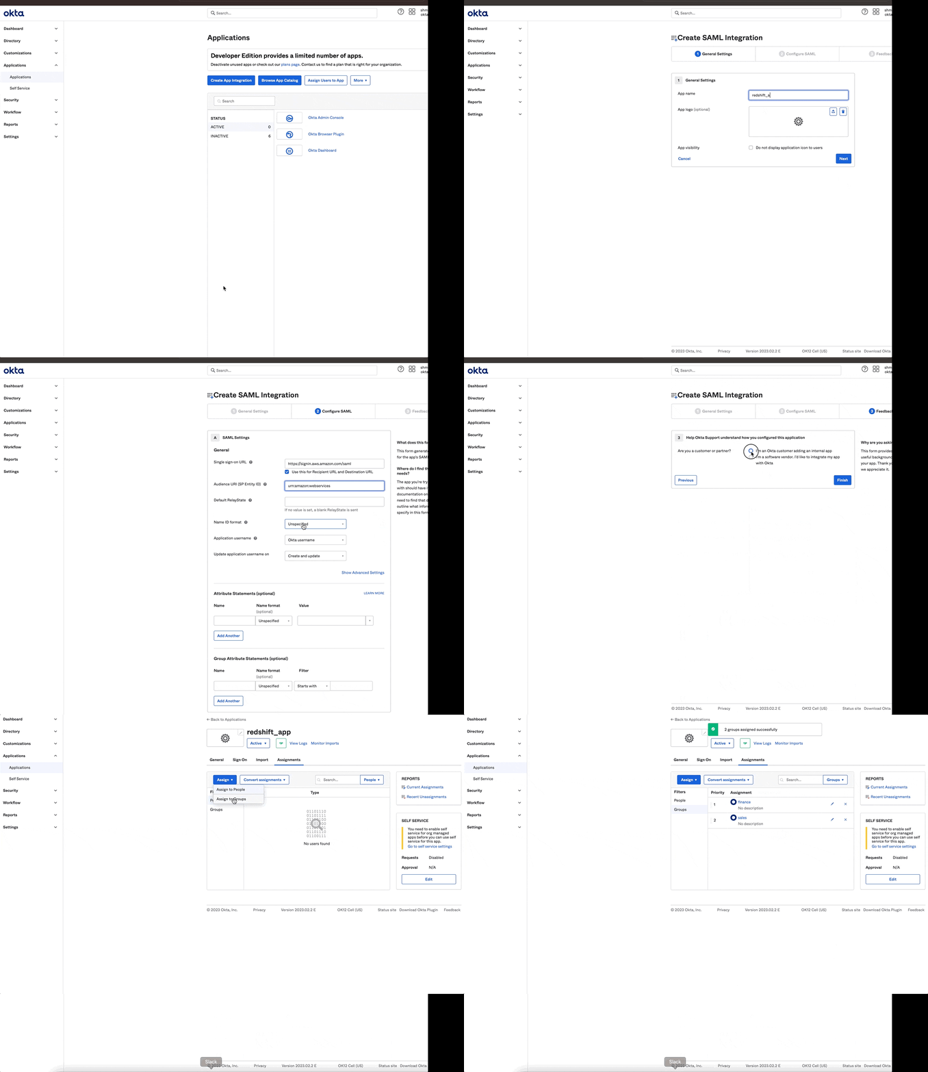
Set up Okta advanced configuration
After you create the custom SAML app, complete the following steps:
- On the admin console, navigate to General and choose Edit under SAML settings.
- Choose Next.
- Set Default Relay State to the Query Editor V2 URL, using the format
https://<region>.console.aws.amazon.com/sqlworkbench/home. For this post, we usehttps://us-west-2.console.aws.amazon.com/sqlworkbench/home. - Under Attribute Statements (optional), add the following properties:
- Provide the IAM role and IdP in comma-separated format using the Role attribute. You’ll create this same IAM role and IdP in a later step when setting up AWS configuration.
- Set
user.loginforRoleSessionName. This is used as an identifier for the temporary credentials that are issued when the role is assumed. - Set the DB roles using
PrincipalTag:RedshiftDbRoles. This uses the Okta groups to fill the principal tags and map them automatically with the Amazon Redshift database roles. Its value must be a colon-separated list in the format role1:role2. - Set
user.loginforPrincipalTag:RedshiftDbUser. This uses the user name in the directory. This is a required tag and defines the database user that is used by Query Editor V2. - Set the transitive keys using
TransitiveTagKeys. This prevents users from changing the session tags in case of role chaining.
The preceding tags are forwarded to the GetCredentials API to get temporary credentials for your Redshift Serverless instance and map automatically with Amazon Redshift database roles. The following table summarizes their attribute statements configuration.
| Name | Name Format | Format | Example |
| https://aws.amazon.com/SAML/Attributes/Role | Unspecified | arn:aws:iam::<yourAWSAccountID>:role/role-name,arn:aws:iam:: <yourAWSAccountID>:saml-provider/provider-name | arn:aws:iam::112034567890:role/oktarole,arn:aws:iam::112034567890:saml-provider/oktaidp |
| https://aws.amazon.com/SAML/Attributes/RoleSessionName | Unspecified | user.login | user.login |
| https://aws.amazon.com/SAML/Attributes/PrincipalTag:RedshiftDbRoles | Unspecified | String.join(":", isMemberOfGroupName("group1") ? 'group1' : '', isMemberOfGroupName("group2") ? 'group2' : '') | String.join(":", isMemberOfGroupName("sales") ? 'sales' : '', isMemberOfGroupName("finance") ? 'finance' : '') |
| https://aws.amazon.com/SAML/Attributes/PrincipalTag:RedshiftDbUser | Unspecified | user.login | user.login |
| https://aws.amazon.com/SAML/Attributes/TransitiveTagKeys | Unspecified | Arrays.flatten("RedshiftDbUser", "RedshiftDbRoles") | Arrays.flatten("RedshiftDbUser", "RedshiftDbRoles") |
- After you add the attribute claims, choose Next followed by Finish.
Your attributes should be in similar format as shown in the following screenshot.
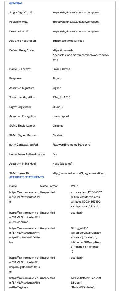
Collect Okta information
To gather your Okta information, complete the following steps:
- On the Sign On tab, choose View SAML setup instructions.

- For Identity Provider Single Sign-on URL, Use this URL when connecting with any third-party SQL client such as SQL Workbench/J.
- Use the IdP metadata in block 4 and save the metadata file in .xml format (for example,
metadata.xml).

Set up AWS configuration
In this section, we provide the steps to configure your IAM resources.
Create the IAM IdP
To create your IAM IdP, complete the following steps:
- On the IAM console, under Access management in the navigation pane, choose Identity providers.
- Choose Add provider.
- For Provider type¸ select SAML.
- For Provider name¸ enter a name.
- Choose Choose file and upload the metadata file (.xml) you downloaded earlier.
- Choose Add provider.

Create the IAM Amazon Redshift access policy
To create your IAM policy, complete the following steps:
- On the IAM console, choose Policies.
- Choose Create policy.
- On the Create policy page, choose the JSON tab.
- For the policy, enter the JSON in following format:
The workgroup ARN is available on the Redshift Serverless workgroup configuration page.
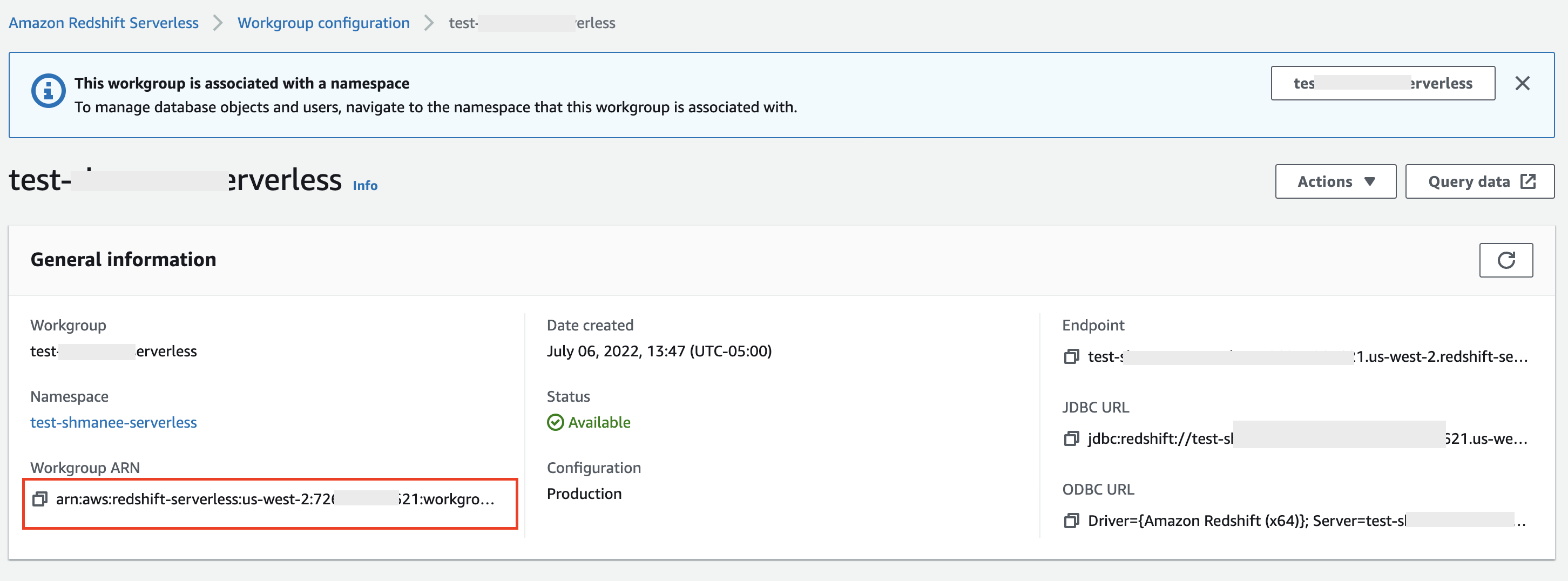
The following example policy includes only a single Redshift Serverless workgroup; you can modify the policy to include multiple workgroups in the Resource section:
- Choose Next: Tags.
- Choose Next: Review.
- In the Review policy section, for Name, enter the name of your policy; for example, OktaRedshiftPolicy.
- For Description, you can optionally enter a brief description of what the policy does.
- Choose Create policy.
Create the IAM role
To create your IAM role, complete the following steps:
- On the IAM console, choose Roles in the navigation pane.
- Choose Create role.
- For Trusted entity type, select SAML 2.0 federation.
- For SAML 2.0-based provider, choose the IdP you created earlier.
- Select Allow programmatic and AWS Management Console access.
- Choose Next.
- Choose the policy you created earlier.
- Also, add the policy
AmazonRedshiftQueryEditorV2ReadSharing. - Choose Next.
- In the Review section, for Role Name, enter the name of your role; for example,
oktarole. - For Description, you can optionally enter a brief description of what the role does.
- Choose Create role.
- Navigate to the role that you just created and choose Trust Relationships.
- Choose Edit trust policy and choose
TagSessionunder Add actions for STS.

When using session tags, trust policies for all roles connected to the IdP passing tags must have the sts:TagSession permission. For roles without this permission in the trust policy, the AssumeRole operation fails.
- Choose Update policy.
The following screenshot shows the role permissions.
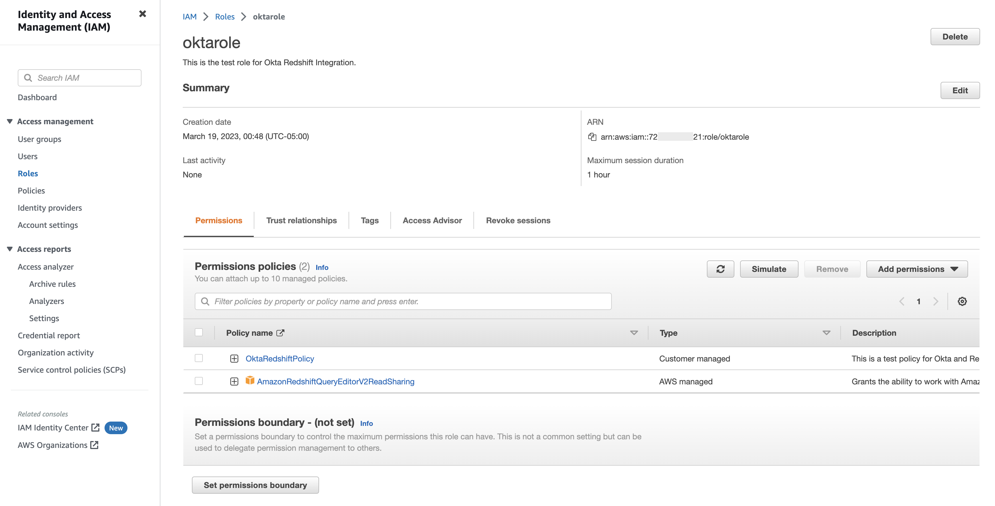
The following screenshot shows the trust relationships.
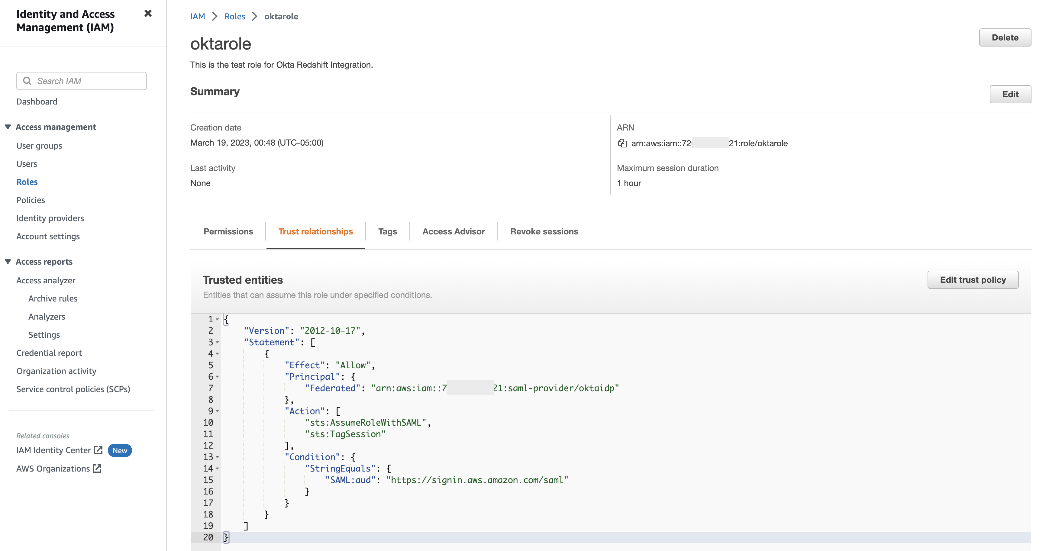
Update the advanced Okta Role Attribute
Complete the following steps:
- Switch back to Okta.com.
- Navigate to the application which you created earlier.
- Navigate to General and click Edit under SAML settings.
- Under Attribute Statements (optional), update the value for the attribute – https://aws.amazon.com/SAML/Attributes/Role, using the actual role and identity provider arn values from the above step. For example,
arn:aws:iam::123456789012:role/oktarole,arn:aws:iam::123456789012:saml-provider/oktaidp.
Configure Redshift Serverless role-based access
In this step, we create database roles in Amazon Redshift based on the groups that you created in Okta. Make sure the role name matches with the Okta Group name.
Amazon Redshift roles simplify managing privileges required for your end-users. In this post, we create two database roles, sales and finance, and grant them access to query tables with sales and finance data, respectively. You can download this sample SQL Notebook and import into Redshift Query Editor v2 to run all cells in the notebook used in this example. Alternatively, you can copy and enter the SQL into your SQL client.
The following is the syntax to create a role in Redshift Serverless:
For example:
Create the sales and finance database schema:
Create the tables:
The following is the syntax to grant permission to the Redshift Serverless role:
Grant relevant permission to the role as per your requirements. In the following example, we grant full permission to the role sales on sales\_schema and only select permission on finance\_schema to the role finance:
Federate to Redshift Serverless using Query Editor V2
The RedshiftDbRoles principal tag and DBGroups are both mechanisms that can be used to integrate with an IdP. However, federating with the RedshiftDbRoles principal has some clear advantages when it comes to connecting with an IdP because it provides automatic mapping between IdP groups and Amazon Redshift database roles. Overall, RedshiftDbRoles is more flexible, easier to manage, and more secure, making it the better option for integrating Amazon Redshift with your IdP.
Now you’re ready to connect to Redshift Serverless using the Query Editor V2 and federated login:
- Use the SSO URL you collected earlier and log in to your Okta account with your user credentials. For this demo, we log in with user Ethan.
- In the Query Editor v2, choose your Redshift Serverless instance (right-click) and choose Create connection.
- For Authentication, select Federated user.
- For Database, enter the database name you want to connect to.
- Choose Create Connection.
User Ethan will be able to access sales\_schema tables. If Ethan tries to access the tables in finance\_schema, he will get a permission denied error.

Configure the SQL client (SQL Workbench/J)
To set up SQL Workbench/J, complete the following steps:
- Create a new connection in SQL Workbench/J and choose Redshift Serverless as the driver.
- Choose Manage drivers and add all the files from the downloaded AWS JDBC driver pack .zip file (remember to unzip the .zip file).
- For Username and Password, enter the values that you set in Okta.

- Capture the values for
app\_id,app\_name, andidp\_hostfrom the Okta app embed link, which can be found on the General tab of your application.

- Set the following extended properties:
- For app\_id, enter the value from app embed link (for example,
0oa8p1o1RptSabT9abd0/avc8k7abc32lL4izh3b8). - For app\_name, enter the value from app embed link (for example,
dev-123456\_redshift\_app\_2). - For idp\_host, enter the value from app embed link (for example,
dev-123456.okta.com). - For plugin\_name, enter
com.amazon.redshift.plugin.OktaCredentialsProvider. The following screenshot shows the SQL Workbench/J extended properties.

- Choose OK.
- Choose Test from SQL Workbench/J to test the connection.
- When the connection is successful, choose OK.
- Choose OK to sign in with the users created.
- For app\_id, enter the value from app embed link (for example,
User Ethan will be able to access the sales\_schema tables. If Ethan tries to access the tables in the finance\_schema, he will get a permission denied error.

Congratulations! You have federated with Redshift Serverless and Okta with SQL Workbench/J using RedshiftDbRoles.
[Optional] Implement MFA with SQL Client and Query Editor V2
Implementing MFA poses an additional challenge because the nature of multi-factor authentication is an asynchronous process between initiating the login (the first factor) and completing the login (the second factor). The SAML response will be returned to the appropriate listener in each scenario; the SQL Client or the AWS console in the case of QEV2. Depending on which login options you will be giving your users, you may need an additional Okta application. See below for the different scenarios:
- If you are ONLY using QEV2 and not using any other SQL client, then you can use MFA with Query Editor V2 with the above application. There are no changes required in the custom SAML application which we have created above.
- If you are NOT using QEV2 and only using third party SQL client (SQL Workbench/J etc), then you need to modify the above custom SAML app as mentioned below.
- If you want to use QEV2 and third-party SQL Client with MFA, then you need create an additional custom SAML app as mentioned below.
Prerequisites for MFA
Each identity provider (IdP) has step for enabling and managing MFA for your users. In the case of Okta, see the following guides on how to enable MFA using the Okta Verify application and by defining an authentication policy.
- Add Okta Verify as an authenticator
- Create an authentication policy
- Add an authentication policy rule
Steps to create/update SAML application which supports MFA for a SQL Client
- If creating a second app, follow all the steps which are described under section 1 (Create Okta SAML application).
- Open the custom SAML app and select General.
- Select Edit under SAML settings
- Click Next in General Settings
- Under General, update the Single sign-on URL to http://localhost:7890/redshift/
- Select Next followed by Finish.
Below is the screenshot from the MFA App after making above changes:

Configure SQL Client for MFA
To set up SQL Workbench/J, complete the following steps:
- Follow all the steps which are described under (Configure the SQL client (SQL Workbench/J))
- Modify your connection updating the extended properties:
- login\_url – Get the Single Sign-on URL as shown in section -Collect Okta information. (For example,
https://dev-123456.okta.com/app/dev-123456\_redshiftapp\_2/abc8p6o5psS6xUhBJ517/sso/saml) - plugin\_name –
com.amazon.redshift.plugin.BrowserSamlCredentialsProvider

- login\_url – Get the Single Sign-on URL as shown in section -Collect Okta information. (For example,
- Choose OK
- Choose OK from SQL Workbench/J. You’re redirected to the browser to sign in with your Okta credentials.
- After that, you will get prompt for MFA. Choose either Enter a code or Get a push notification.

- Once authentication is successful, log in to be redirected to a page showing the connection as successful.

- With this connection profile, run the following query to return federated user name.

Troubleshooting
If your connection didn’t work, consider the following:
- Enable logging in the driver. For instructions, see Configure logging.
- Make sure to use the latest Amazon Redshift JDBC driver version.
- If you’re getting errors while setting up the application on Okta, make sure you have admin access.
- If you can authenticate via the SQL client but get a permission issue or can’t see objects, grant the relevant permission to the role, as detailed earlier in this post.
Clean up
When you’re done testing the solution, clean up the resources to avoid incurring future charges:
- Delete the Redshift Serverless instance by deleting both the workgroup and the namespace.
- Delete the IAM roles, IAM IdPs, and IAM policies.
Conclusion
In this post, we provided step-by-step instructions to integrate Redshift Serverless with Okta using the Amazon Redshift Query Editor V2 and SQL Workbench/J with the help of federated IAM roles and automatic database-role mapping. You can use a similar setup with any other SQL client (such as DBeaver or DataGrip) or business intelligence tool (such as Tableau Desktop). We also showed how Okta group membership is mapped automatically with Redshift Serverless roles to use role-based authentication seamlessly.
For more information about Redshift Serverless single sign-on using database roles, see Defining database roles to grant to federated users in Amazon Redshift Serverless.
About the Authors
 Maneesh Sharma is a Senior Database Engineer at AWS with more than a decade of experience designing and implementing large-scale data warehouse and analytics solutions. He collaborates with various Amazon Redshift Partners and customers to drive better integration.
 Debu Panda is a Senior Manager, Product Management at AWS. He is an industry leader in analytics, application platform, and database technologies, and has more than 25 years of experience in the IT world.
 Mohamed Shaaban is a Senior Software Engineer in Amazon Redshift and is based in Berlin, Germany. He has over 12 years of experience in the software engineering. He is passionate about cloud services and building solutions that delight customers. Outside of work, he is an amateur photographer who loves to explore and capture unique moments.
 Rajiv Gupta is Sr. Manager of Analytics Specialist Solutions Architects based out of Irvine, CA. He has 20+ years of experience building and managing teams who build data warehouse and business intelligence solutions.
 Amol Mhatre is a Database Engineer in Amazon Redshift and works on Customer & Partner engagements. Prior to Amazon, he has worked on multiple projects involving Database & ERP implementations.
 Ning Di is a Software Development Engineer at Amazon Redshift, driven by a genuine passion for exploring all aspects of technology.
 Harsha Kesapragada is a Software Development Engineer for Amazon Redshift with a passion to build scalable and secure systems. In the past few years, he has been working on Redshift Datasharing, Security and Redshift Serverless.
This post is a guest post co-written with SeonJeong Lee, JaeRyun Yim, and HyeonSeok Yang from Encored Technologies.
Encored Technologies (Encored) is an energy IT company in Korea that helps their customers generate higher revenue and reduce operational costs in renewable energy industries by providing various AI-based solutions. Encored develops machine learning (ML) applications predicting and optimizing various energy-related processes, and their key initiative is to predict the amount of power generated at renewable energy power plants.
In this post, we share how Encored runs data engineering pipelines for containerized ML applications on AWS and how they use AWS Lambda to achieve performance improvement, cost reduction, and operational efficiency. We also demonstrate how to use AWS services to ingest and process GRIB (GRIdded Binary) format data, which is a file format commonly used in meteorology to store and exchange weather and climate data in a compressed binary form. It allows for efficient data storage and transmission, as well as easy manipulation of the data using specialized software.
Business and technical challenge
Encored is expanding their business into multiple countries to provide power trading services for end customers. The amount of data and the number of power plants they need to collect data are rapidly increasing over time. For example, the volume of data required for training one of the ML models is more than 200 TB. To meet the growing requirements of the business, the data science and platform team needed to speed up the process of delivering model outputs. As a solution, Encored aimed to migrate existing data and run ML applications in the AWS Cloud environment to efficiently process a scalable and robust end-to-end data and ML pipeline.
Solution overview
The primary objective of the solution is to develop an optimized data ingestion pipeline that addresses the scaling challenges related to data ingestion. During its previous deployment in an on-premises environment, the time taken to process data from ingestion to preparing the training dataset exceeded the required service level agreement (SLA). One of the input datasets required for ML models is weather data supplied by the Korea Meteorological Administration (KMA). In order to use the GRIB datasets for the ML models, Encored needed to prepare the raw data to make it suitable for building and training ML models. The first step was to convert GRIB to the Parquet file format.
Encored used Lambda to run an existing data ingestion pipeline built in a Linux-based container image. Lambda is a compute service that lets you run code without provisioning or managing servers. Lambda runs your code on a high-availability compute infrastructure and performs all of the administration of the compute resources, including server and operating system maintenance, capacity provisioning and automatic scaling, and logging. AWS Lambda is triggered to ingest and process GRIB data files when they are uploaded to Amazon Simple Storage Service (Amazon S3). Once the files are processed, they are stored in Parquet format in the other S3 bucket. Encored receives GRIB files throughout the day, and whenever new files arrive, an AWS Lambda function runs a container image registered in Amazon Elastic Container Registry (ECR). This event-based pipeline triggers a customized data pipeline that is packaged in a container-based solution. Leveraging Amazon AWS Lambda, this solution is cost-effective, scalable, and high-performing.Encored uses Python as their preferred language.
The following diagram illustrates the solution architecture.
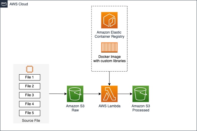
For data-intensive tasks such as extract, transform, and load (ETL) jobs and ML inference, Lambda is an ideal solution because it offers several key benefits, including rapid scaling to meet demand, automatic scaling to zero when not in use, and S3 event triggers that can initiate actions in response to object-created events. All this contributes to building a scalable and cost-effective data event-driven pipeline. In addition to these benefits, Lambda allows you to configure ephemeral storage (/tmp) between 512–10,240 MB. Encored used this storage for their data application when reading or writing data, enabling them to optimize performance and cost-effectiveness. Furthermore, Lambda’s pay-per-use pricing model means that users only pay for the compute time in use, making it a cost-effective solution for a wide range of use cases.
Prerequisites
For this walkthrough, you should have the following:
- An AWS account
- The AWS Command Line Interface (AWS CLI) installed
- The Docker CLI
- Your function codes
Build your application required for your Docker image
The first step is to develop an application that can ingest and process files. This application reads the bucket name and object key passed from a trigger added to Lambda function. The processing logic involves three parts: downloading the file from Amazon S3 into ephemeral storage (/tmp), parsing the GRIB formatted data, and saving the parsed data to Parquet format.
The customer has a Python script (for example, app.py) that performs these tasks as follows:
Prepare a Docker file
The second step is to create a Docker image using an AWS base image. To achieve this, you can create a new Dockerfile using a text editor on your local machine. This Dockerfile should contain two environment variables:
LAMBDA\_TASK\_ROOT=/var/taskLAMBDA\_RUNTIME\_DIR=/var/runtime
It’s important to install any dependencies under the ${LAMBDA\_TASK\_ROOT} directory alongside the function handler to ensure that the Lambda runtime can locate them when the function is invoked. Refer to the available Lambda base images for custom runtime for more information.
Build a Docker image
The third step is to build your Docker image using the docker build command. When running this command, make sure to enter a name for the image. For example:
docker build -t process-grib .
In this example, the name of the image is process-grib. You can choose any name you like for your Docker image.
Upload the image to the Amazon ECR repository
Your container image needs to reside in an Amazon Elastic Container Registry (Amazon ECR) repository. Amazon ECR is a fully managed container registry offering high-performance hosting, so you can reliably deploy application images and artifacts anywhere. For instructions on creating an ECR repository, refer to Creating a private repository.
The first step is to authenticate the Docker CLI to your ECR registry as follows:
The second step is to tag your image to match your repository name, and deploy the image to Amazon ECR using the docker push command:
Deploy Lambda functions as container images
To create your Lambda function, complete the following steps:
- On the Lambda console, choose Functions in the navigation pane.
- Choose Create function.
- Choose the Container image option.
- For Function name, enter a name.
- For Container image URI, provide a container image. You can enter the ECR image URI or browse for the ECR image.
- Under Container image overrides, you can override configuration settings such as the entry point or working directory that are included in the Dockerfile.
- Under Permissions, expand Change default execution role.
- Choose to create a new role or use an existing role.
- Choose Create function.
Key considerations
To handle a large amount of data concurrently and quickly, Encored needed to store GRIB formatted files in the ephemeral storage (/tmp) that comes with Lambda. To achieve this requirement, Encored used tempfile.NamedTemporaryFile, which allows users to create temporary files easily that are deleted when no longer needed. With Lambda, you can configure ephemeral storage between 512 MB–10,240 MB for reading or writing data, allowing you to run ETL jobs, ML inference, or other data-intensive workloads.
Business outcome
Hyoseop Lee (CTO at Encored Technologies) said, “Encored has experienced positive outcomes since migrating to AWS Cloud. Initially, there was a perception that running workloads on AWS would be more expensive than using an on-premises environment. However, we discovered that this was not the case once we started running our applications on AWS. One of the most fascinating aspects of AWS services is the flexible architecture options it provides for processing, storing, and accessing large volumes of data that are only required infrequently.”
Conclusion
In this post, we covered how Encored built serverless data pipelines with Lambda and Amazon ECR to achieve performance improvement, cost reduction, and operational efficiency.
Encored successfully built an architecture that will support their global expansion and enhance technical capabilities through AWS services and the AWS Data Lab program. Based on the architecture and various internal datasets Encored has consolidated and curated, Encored plans to provide renewable energy forecasting and energy trading services.
Thanks for reading this post and hopefully you found it useful. To accelerate your digital transformation with ML, AWS is available to support you by providing prescriptive architectural guidance on a particular use case, sharing best practices, and removing technical roadblocks. You’ll leave the engagement with an architecture or working prototype that is custom fit to your needs, a path to production, and deeper knowledge of AWS services. Please contact your AWS Account Manager or Solutions Architect to get started. If you don’t have an AWS Account Manager, please contact Sales.
To learn more about ML inference use cases with Lambda, check out the following blog posts:
- Machine learning inference at scale using AWS serverless
- Deploy a machine learning inference data capture solution on AWS Lambda
These resources will provide you with valuable insights and practical examples of how to use Lambda for ML inference.
About the Authors
 SeonJeong Lee is the Head of Algorithms at Encored. She is a data practitioner who finds peace of mind from beautiful codes and formulas.
 JaeRyun Yim is a Senior Data Scientist at Encored. He is striving to improve both work and life by focusing on simplicity and essence in my work.
 HyeonSeok Yang is the platform team lead at Encored. He always strives to work with passion and spirit to keep challenging like a junior developer, and become a role model for others.
 Younggu Yun works at AWS Data Lab in Korea. His role involves helping customers across the APAC region meet their business objectives and overcome technical challenges by providing prescriptive architectural guidance, sharing best practices, and building innovative solutions together.
Welcome to the era of data. The sheer volume of data captured daily continues to grow, calling for platforms and solutions to evolve. Services such as Amazon Simple Storage Service (Amazon S3) offer a scalable solution that adapts yet remains cost-effective for growing datasets. The Amazon Sustainability Data Initiative (ASDI) uses the capabilities of Amazon S3 to provide a no-cost solution for you to store and share climate science workloads across the globe. Amazon’s Open Data Sponsorship Program allows organizations to host free of charge on AWS.
Over the last decade, we’ve seen a surge in data science frameworks coming to fruition, along with mass adoption by the data science community. One such framework is Dask, which is powerful for its ability to provision an orchestration of worker compute nodes, thereby accelerating complex analysis on large datasets.
In this post, we show you how to deploy a custom AWS Cloud Development Kit (AWS CDK) solution that extends Dask’s functionality to work inter-Regionally across Amazon’s global network. The AWS CDK solution deploys a network of Dask workers across two AWS Regions, connecting into a client Region. For more information, refer to Guidance for Distributed Computing with Cross Regional Dask on AWS and the GitHub repo for open-source code.
After deployment, the user will have access to a Jupyter notebook, where they can interact with two datasets from ASDI on AWS: Coupled Model Intercomparison Project 6 (CMIP6) and ECMWF ERA5 Reanalysis. CMIP6 focuses on the sixth phase of global coupled ocean-atmosphere general circulation model ensemble; ERA5 is the fifth generation of ECMWF atmospheric reanalyses of the global climate, and the first reanalysis produced as an operational service.
This solution was inspired by work with a key AWS customer, the UK Met Office. The Met Office was founded in 1854 and is the national meteorological service for the UK. They provide weather and climate predictions to help you make better decisions to stay safe and thrive. A collaboration between the Met Office and EUMETSAT, detailed in Data Proximate Computation on a Dask Cluster Distributed Between Data Centres, highlights the growing need to develop a sustainable, efficient, and scalable data science solution. This solution achieves this by bringing compute closer to the data, rather than forcing the data to come closer to compute resources, which adds cost, latency, and energy.
Solution overview
Each day, the UK Met Office produces up to 300 TB of weather and climate data, a portion of which is published to ASDI. These datasets are distributed across the world and hosted for public use. The Met Office would like to enable consumers to make the more of their data to help inform critical decisions on addressing issues such as better preparation for climate change-induced wildfires and floods, and reducing food insecurity through better crop yield analysis.
Traditional solutions in use today, particularly with climate data, are time consuming and unsustainable, replicating datasets cross Regions. Unnecessary data transfer on the petabyte scale is costly, slow, and consumes energy.
We estimated that if this practice were adopted by the Met Office users, the equivalent of 40 homes’ daily power consumption could be saved every day, and they could also reduce the transfer of data between regions.
The following diagram illustrates the solution architecture.

The solution can be broken into three major segments: client, workers, and network. Let’s dive into each and see how they come together.
Client
The client represents the source Region where data scientists connect. This Region (Region A in the diagram) contains an Amazon SageMaker notebook, an Amazon OpenSearch Service domain, and a Dask scheduler as key components. System administrators have access to the built-in Dask dashboard exposed via an Elastic Load Balancer.
Data scientists have access to the Jupyter notebook hosted on SageMaker. The notebook is able to connect and run workloads on the Dask scheduler. The OpenSearch Service domain stores metadata on the datasets connected at the Regions. Notebook users can query this service to retrieve details such as the correct Region of Dask workers without needing to know the data’s Regional location beforehand.
Worker
Each of the worker Regions (Regions B and C in the diagram) is comprised of an Amazon Elastic Container Service (Amazon ECS) cluster of Dask workers, an Amazon FSx for Lustre file system, and a standalone Amazon Elastic Compute Cloud (Amazon EC2) instance. FSx for Lustre allows Dask workers to access and process Amazon S3 data from a high-performance file system by linking your file systems to S3 buckets. It provides sub-millisecond latencies, up to hundreds of GBs/s of throughput, and millions of IOPS. A key feature of Lustre is that only the file system’s metadata is synced. Lustre manages the balance of files to be loaded in and kept warm, based on demand.
Worker clusters scale based on CPU usage, provision additional workers in extended periods of demand, and scale down as resources become idle.
Each night at 0:00 UTC, a data sync job prompts the Lustre file system to resync with the attached S3 bucket, and pulls an up-to-date metadata catalog of the bucket. Subsequently, the standalone EC2 instance pushes these updates into OpenSearch Service respective to that Region’s index. OpenSearch Service provides the necessary information to the client as to which pool of workers should be called upon for a particular dataset.
Network
Networking forms the crux of this solution, utilizing Amazon’s internal backbone network. By using AWS Transit Gateway, we’re able to connect each of the Regions to each other without needing to traverse the public internet. Each of the workers are able to connect dynamically into the Dask scheduler, allowing data scientists to run inter-regional queries through Dask.
Prerequisites
The AWS CDK package uses the TypeScript programming language. Follow the steps in Getting Started for AWS CDK to set up your local environment and bootstrap your development account (you’ll need to bootstrap all Regions specified in the GitHub repo).
For a successful deployment, you’ll need Docker installed and running on your local machine.
Deploy the AWS CDK package
Deploying an AWS CDK package is straightforward. After you install the prerequisites and bootstrap your account, you can proceed with downloading the code base.
- Download the GitHub repository:
- Install node modules:
- Deploy the AWS CDK:
The stack can take over an hour and a half to deploy.
Code walkthrough
In this section, we inspect some of the key features of the code base. If you’d like to inspect the full code base, refer to the GitHub repository.
Configure and customize your stack
In the file bin/variables.ts, you’ll find two variable declarations: one for the client and one for workers. The client declaration is a dictionary with a reference to a Region and CIDR range. Customizing these variables will change both the Region and CIDR range of where client resources will deploy.
The worker variable copies this same functionality; however, it’s a list of dictionaries to accommodate adding or subtracting datasets the user wishes to include. Additionally, each dictionary contains the added fields of dataset and lustreFileSystemPath. Dataset is used to specify the connecting S3 URI for Lustre to connect to. The lustreFileSystemPath variable is used as a mapping for how the user wants that dataset to map locally on the worker file system. See the following code:
Dynamically publish the scheduler IP
A challenge inherent to the cross-Regional nature of this project was maintaining a dynamic connection between the Dask workers and the scheduler. How could we publish an IP address, which is capable of changing, across AWS Regions? We were able to accomplish this through the use of AWS Cloud Map and associate-vpc-with-hosted-zone. The service abstracts allowing AWS to manage this DNS namespace privately. See the following code:
Jupyter notebook UI
The Jupyter notebook hosted on SageMaker provides scientists with a ready-made environment for deployment to easily connect and experiment on the loaded datasets. We used a lifecycle configuration script to provision the notebook with a preconfigured developer environment and example code base. See the following code:
Dask worker nodes
When it comes to the Dask workers, greater customizability is provided, more specifically on instance type, threads per container, and scaling alarms. By default, the workers provision on instance type m5d.4xlarge, mount to the Lustre file system on launch, and subdivide its workers and threads dynamically to ports. All this is optionally customizable. See the following code:
Performance
To assess performance, we use a sample computation and plotting of air temperature at 2 meters based on the difference between CMIP6 prediction for a month and ERA5 mean air temperature for 10 years. We set a benchmark of two workers in each Region and assess the difference in time reduction as additional workers were added. In theory, as the solution scales, there should be a productive material difference in reducing overall time.
The following table summarizes our dataset details.
| Dataset | Variables | Disk Size | Xarray Dataset Size | Region |
| ERA5 | 2011–2020 (120 netcdf files) | 53.5GB | 364.1 GB | us-east-1 |
| CMIP6 | 1.13GB | 0.11 GB | us-west-2 |
The following table shows the results collected, showcasing the time (in seconds) for each computation and prediction in three stages in computing CMIP6 prediction, ERA5, and difference.
| . | . | Number of Workers | |||
| Compute | Region | 2(CMIP) + 2(ERA) | 2(CMIP) + 4(ERA) | 2(CMIP) + 8(ERA) | 2(CMIP) + 12(ERA) |
CMIP6 (predicted\_tas\_regridded) | us-west-2 | 11.8 | 11.5 | 11.2 | 11.6 |
ERA5 (historic\_temp\_regridded) | us-east-1 | 1512 | 711 | 427 | 202 |
Difference (propogated pool) | us-west-2 and us-east-1 | 1527 | 906 | 469 | 251 |
The following graph visualizes the performance and scale.
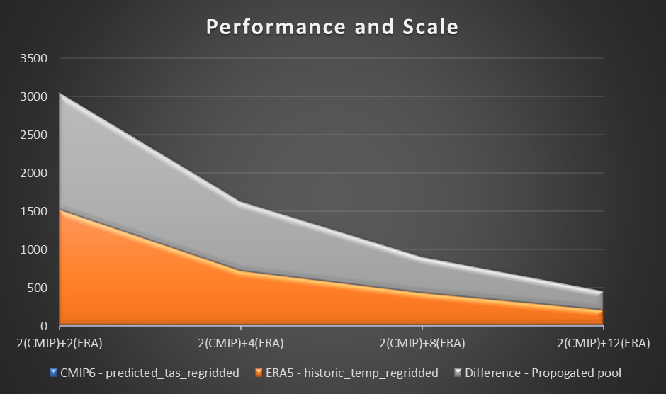
From our experiment, we observed a linear improvement on computation for the ERA5 dataset as the number of workers increased. As the numbers of workers increased, computation times were at times halved.
Jupyter notebook
As part of the solution launch, we deploy a preconfigured Jupyter notebook to help test the cross-Regional Dask solution. The notebook demonstrates the removed worry of needing to know the Regional location of datasets, instead querying a catalog through a series of Jupyter notebooks running in the background.
To get started, follow the instructions in this section.
The code for the notebooks can be found in lib/SagemakerCode with the primary notebook being ux\_notebook.ipynb. This notebook calls upon other notebooks, triggering helper scripts. ux\_notebook is designed to be the entry point for scientists, without the need for going elsewhere.
To get started, open this notebook in SageMaker after you have deployed the AWS CDK. The AWS CDK creates a notebook instance with all of the files in the repository loaded and backed up to an AWS CodeCommit repository.
To run the application, open and run the first cell of ux\_notebook. This cell runs the get\_variables notebook in the background, which prompts you for an input for the data you would like to select. We include an example; however, note that questions will only appear after the previous option has been selected. This is intentional in limiting the drop-down choices and is optionally configurable by editing the get\_variables notebook.
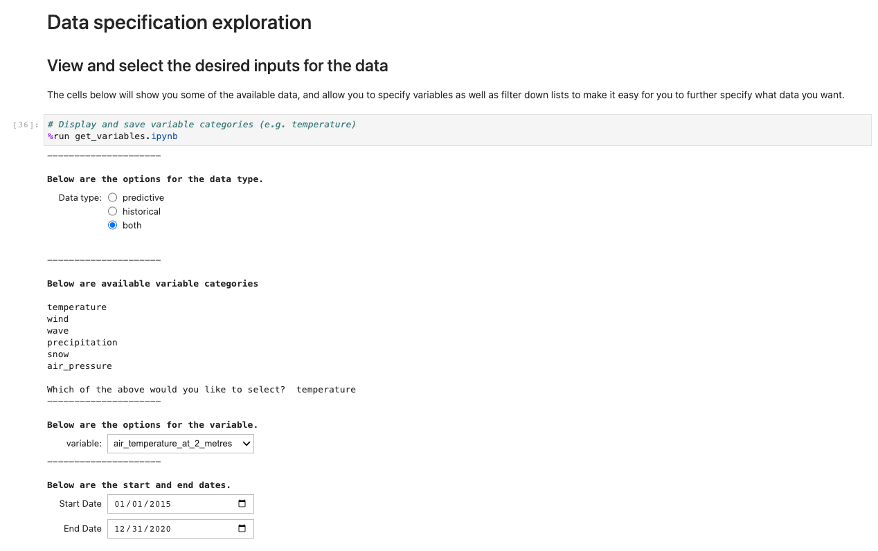
The preceding code stores variables globally so that other notebooks can retrieve and load your selection of choices. For demonstration, the next cell should output the save variables from before.
Next, a prompt for further data specifications appears. This cell refines the data you’re after by presenting the IDs of tables in human-readable format. Users select as if it were a form, but the titles map to tables in the background that help the system retrieve the appropriate datasets.
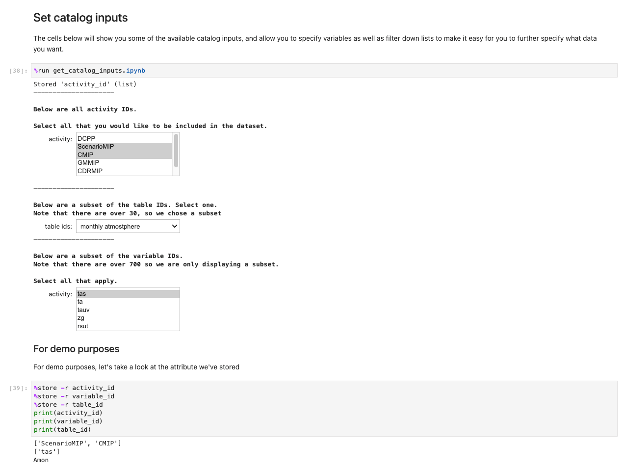
After you have stored all your choices and selection cells, load the data into the Regions by running the cell in the Getting the data set section. The %%capture command will suppress unnecessary outputs from the get\_data notebook. Note you may remove this to inspect outputs from the other notebooks. Data is then retrieved in the backend.
While other notebooks are being run in the background, the only touchpoint for the user is the ux\_notebook. This is to abstract the tedious process of importing data into a format any user is able to follow with ease.
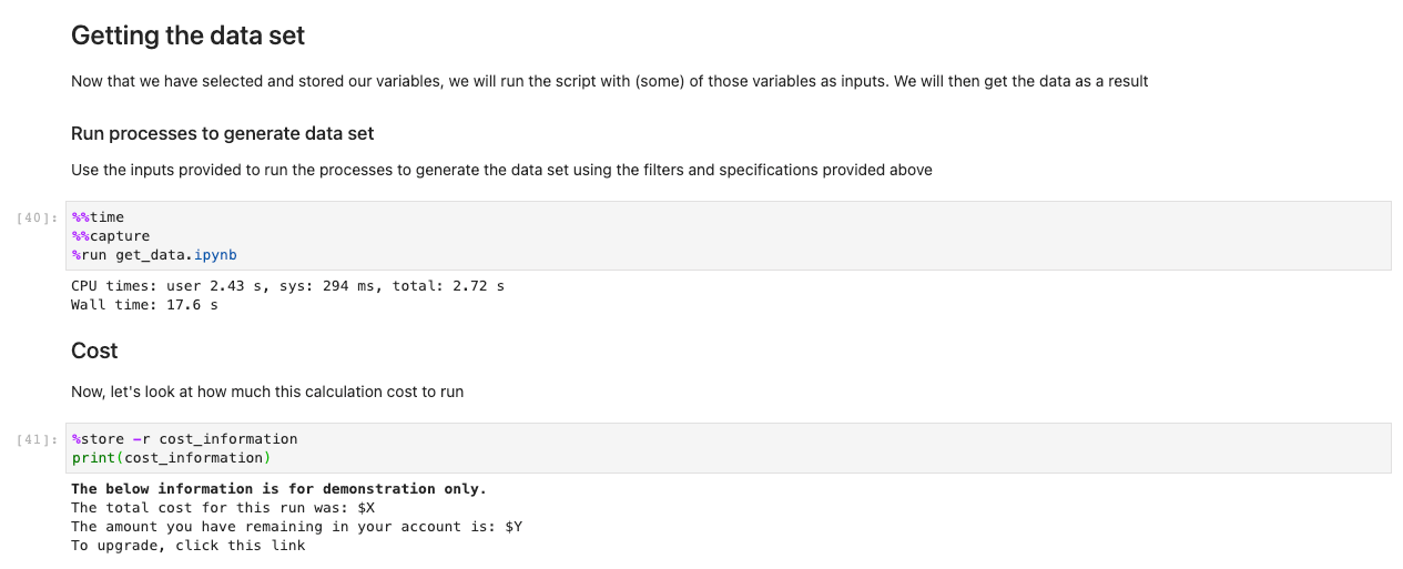
With the data now loaded, we can start interacting with it. The following cells are examples of calculations you may run on weather data. Using xarrays, we import, calculate, and then plot those datasets.
Our sample illustrates a plot of predictive data retrieving data, running the computation, and plotting the results in under 7.5 seconds—orders of magnitude faster than a typical approach.
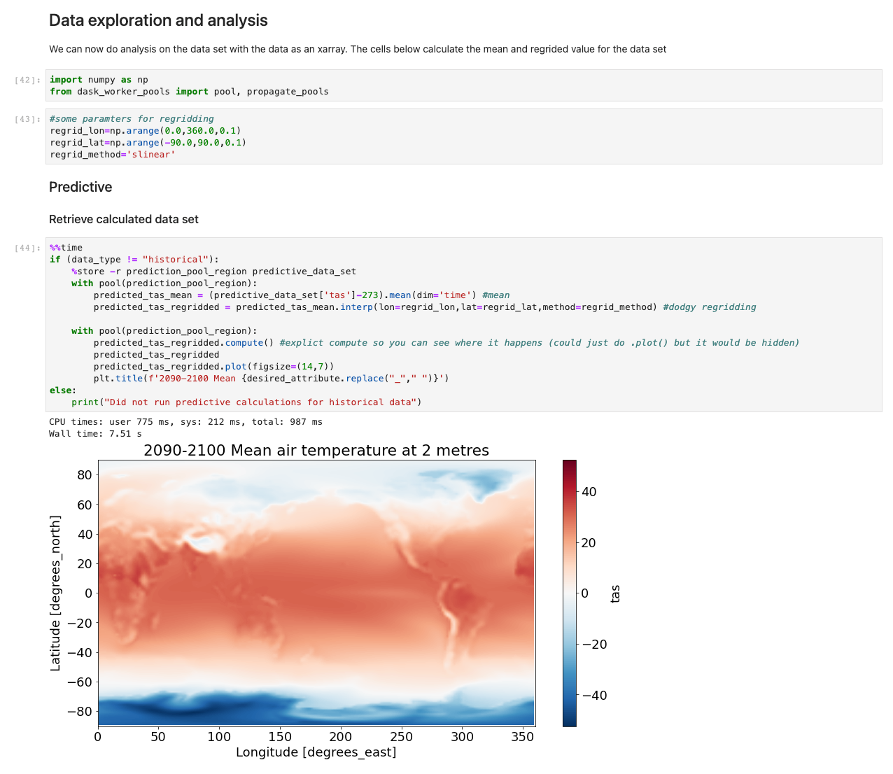
Under the hood
The notebooks get\_catalog\_input and get\_variables use the library ipywidgets to display widgets such as drop-downs and multi-box selections. These options are saved globally using the %%store command so that they can be accessed from the ux\_notebook. One of the options prompts you on whether you want historical data, predictive data, or both. This variable is passed to the get\_data notebook to determine which subsequent notebooks to run.
The get\_data notebook first retrieves the shared OpenSearch Service domain saved to AWS Systems Manager Parameter Store. This domain allows our notebook to run a query on collecting information that will indicate where the selected datasets are stored Regionally. With those datasets located Regionally, the notebook will make a connection attempt to the Dask scheduler, passing the information collected from OpenSearch Service. The Dask scheduler in turn will be able to call on workers in the correct Regions.
How to customize and continue development
These notebooks are meant to be an example of how you can create a way for users to interface and interact with the data. The notebook in this post serves as an illustration for what’s possible, and we invite you to continue building upon the solution to further improve user engagement. The core part of this solution is the backend technology, but without some mechanism to interact with that backend, users won’t realize the full potential of the solution.
Clean up
To avoid incurring future charges, delete the resources. Let’s destroy our deployed solution with the following command:
Conclusion
This post showcases the extension of Dask inter-Regionally on AWS, and a possible integration with public datasets on AWS. The solution was built as a generic pattern, and further datasets can be loaded in to accelerate high I/O analyses on complex data.
Data is transforming every field and every business. However, with data growing faster than most companies can keep track of, collecting data and getting value out of that data is challenging. A modern data strategy can help you create better business outcomes with data. AWS provides the most complete set of services for the end-to-end data journey to help you unlock value from your data and turn it into insight.
To learn more about the various ways to use your data on the cloud, visit the AWS Big Data Blog. We further invite you to comment with your thoughts on this post, and whether this is a solution you plan on trying out.
About the Authors
 Patrick O’Connor is a WWSO Prototyping Engineer based in London. He is a creative problem-solver, adaptable across a wide range of technologies, such as IoT, serverless tech, 3D spatial tech, and ML/AI, along with a relentless curiosity on how technology can continue to evolve everyday approaches.
 Chakra Nagarajan is a Principal Machine Learning Prototyping SA with 21 years of experience in machine learning, big data, and high-performance computing. In his current role, he helps customers solve real-world complex business problems by building prototypes with end-to-end AI/ML solutions in cloud and edge devices. His ML specialization includes computer vision, natural language processing, time series forecasting, and personalization.
 Val Cohen is a senior WWSO Prototyping Engineer based in London. A problem solver by nature, Val enjoys writing code to automate processes, build customer obsessed tools, and create infrastructure for various applications for her global customer base. Val has experience across a wide variety of technologies, such as front-end web development, backend work, and AI/ML.
 Niall Robinson is Head of product futures at the UK Met Office. He and his team explore new ways the Met Office can provide value through product innovation and strategic partnerships. He’s had a varied career, leading a multidisciplinary informatics R&D team, academic research in data science, and field scientist along with climate modeler expertise.
Amazon EMR on Amazon EKS is a deployment option offered by Amazon EMR that enables you to run Apache Spark applications on Amazon Elastic Kubernetes Service (Amazon EKS) in a cost-effective manner. It uses the EMR runtime for Apache Spark to increase performance so that your jobs run faster and cost less.
Apache Spark allows you to configure the amount of Memory and vCPU cores that a job will utilize. However, tuning these values is a manual process that can be complex and ripe with pitfalls. For example, allocating too little memory can result in out-of-memory exceptions and poor job reliability. On the other hand, too much can result in over-spending on idle resources, poor cluster utilization and high costs. Moreover, it’s hard to right-size these settings for some use cases such as interactive analytics due to lack of visibility into future requirements. In the case of recurring jobs, keeping these settings up to date taking into account changing load patterns (due to external seasonal factors for instance) remains a challenge.
To address this, Amazon EMR on EKS has recently announced support for vertical autoscaling, a feature that uses the Kubernetes Vertical Pod Autoscaler (VPA) to automatically tune the memory and CPU resources of EMR Spark applications to adapt to the needs of the provided workload, simplifying the process of tuning resources and optimizing costs for these applications. You can use vertical autoscaling’s ability to tune resources based on historic data to keep memory and CPU settings up to date even when the profile of the workload varies over time. Additionally, you can use its ability to react to real-time signals to enable applications recover from out-of-memory (OOM) exceptions, helping improve job reliability.
Vertical autoscaling vs existing autoscaling solutions
Vertical autoscaling complements existing Spark autoscaling solutions such as Dynamic Resource Allocation (DRA) and Kubernetes autoscaling solutions such as Karpenter.
Features such as DRA typically work on the horizontal axis, where an increase in load results in an increase in the number of Kubernetes pods that will process the load. In the case of Spark, this results in data being processed across additional executors. When DRA is enabled, Spark starts with an initial number of executors and scales this up if it observes that there are tasks sitting and waiting for executors to run on. DRA works at the pod level and would need an underlying cluster-level auto-scaler such as Karpenter to bring in additional nodes or scale down unused nodes in response to these pods getting created and deleted.
However, for a given data profile and a query plan, sometimes the parallelism and the number of executors can’t be easily changed. As an example, if you’re attempting to join two tables that store data already sorted and bucketed by the join keys, Spark can efficiently join the data by using a fixed number of executors that equals the number of buckets in the source data. Since the number of executors cannot be changed, vertical autoscaling can help here by offering additional resources or scaling down unused resources at the executor level. This has a few advantages:
- If a pod is optimally sized, the Kubernetes scheduler can efficiently pack in more pods in a single node, leading to better utilization of the underlying cluster.
- The Amazon EMR on EKS uplift is charged based on the vCPU and memory resources consumed by a Kubernetes pod.This means an optimally sized pod is cheaper.
How vertical autoscaling works
Vertical autoscaling is a feature that you can opt into at the time of submitting an EMR on EKS job. When enabled, it uses VPA to track the resource utilization of your EMR Spark jobs and derive recommendations for resource assignments for Spark executor pods based on this data. The data, fetched from the Kubernetes Metric Server, feeds into statistical models that VPA constructs in order to build recommendations. When new executor pods spin up belonging to a job that has vertical autoscaling enabled, they’re autoscaled based on this recommendation, ignoring the usual sizing done via Spark’s executor memory configuration (controlled by the spark.executor.memory Spark setting).
Vertical autoscaling does not impact pods that are running, since in-place resizing of pods remains unsupported as of Kubernetes version 1.26, the latest supported version of Kubernetes on Amazon EKS as of this writing. However, it’s useful in the case of a recurring job where we can perform autoscaling based on historic data as well as scenarios when some pods go out-of-memory and get re-started by Spark, where vertical autoscaling can be used to selectively scale up the re-started pods and facilitate automatic recovery.
Data tracking and recommendations
To recap, vertical autoscaling uses VPA to track resource utilization for EMR jobs. For a deep-dive into the functionality, refer to the VPA Github repo. In short, vertical autoscaling sets up VPA to track the container\_memory\_working\_set\_bytes metric for the Spark executor pods that have vertical autoscaling enabled.
Real-time metric data is fetched from the Kubernetes Metric Server. By default, vertical autoscaling tracks the peak memory working set size for each pod and makes recommendations based on the p90 of the peak with a 40% safety margin added in. It also listens to pod events such as OOM events and reacts to these events. In the case of OOM events, VPA automatically bumps up the recommended resource assignment by 20%.
The statistical models, which also represent historic resource utilization data are stored as custom resource objects on your EKS cluster. This means that deleting these objects also purges old recommendations.
Customized recommendations through job signature
One of the major use-cases of vertical autoscaling is to aggregate usage data across different runs of EMR Spark jobs to derive resource recommendations. To do so, you need to provide a job signature. This can be a unique name or identifier that you configure at the time of submitting your job. If your job recurs at a fixed schedule (such as daily or weekly), it’s important that your job signature doesn’t change for each new instance of the job in order for VPA to aggregate and compute recommendations across different runs of the job.
A job signature can be the same even across different jobs if you believe they’ll have similar resource profiles. You can therefore use the signature to combine tracking and resource modeling across different jobs that you expect to behave similarly. Conversely, if a job’s behavior is changing at some point in time, such as due to a change in the upstream data or the query pattern, you can easily purge the old recommendations by either changing your signature or deleting the VPA custom resource for this signature (as explained later in this post).
Monitoring mode
You can use vertical autoscaling in a monitoring mode where no autoscaling is actually performed. Recommendations are reported to Prometheus if you have that setup on your cluster and you can monitor the recommendations through Grafana dashboards and use that to debug and make manual changes to the resource assignments. Monitoring mode is the default but you can override and use one of the supported autoscaling modes as well at the time of submitting a job. Refer to documentation for usage and a walkthrough on how to get started.
Monitoring vertical autoscaling through kubectl
You can use the Kubernetes command-line tool kubectl to list active recommendations on your cluster, view all the job signatures that are being tracked as well as purge resources associated with signatures that aren’t relevant anymore. In this section, we provide some example code to demonstrate listing, querying, and deleting recommendations.
List all vertical autoscaling recommendations on a cluster
You can use kubectl to get the verticalpodautoscaler resource in order to view the current status and recommendations. The following sample query lists all resources currently active on your EKS cluster:
This produces output similar to the following
Query and delete a recommendation
You can also use kubectl to purge recommendation for a job based on the signature. Alternately, you can use the --all flag and skip specifying the signature to purge all the resources on your cluster. Note that in this case you’ll actually be deleting the EMR vertical autoscaling job-run resource. This is a custom resource managed by EMR, deleting it automatically deletes the associated VPA object that tracks and stores recommendations. See the following code:
You can use the --all and --all-namespaces to delete all vertical autoscaling related resources
Monitor vertical autoscaling through Prometheus and Grafana
You can use Prometheus and Grafana to monitor the vertical autoscaling functionality on your EKS cluster. This includes viewing recommendations that evolve over time for different job signatures, monitoring the autoscaling functionality etc. For this setup, we assume Prometheus and Grafana are already installed on your EKS cluster using the official Helm charts. If not, refer to the Setting up Prometheus and Grafana for monitoring the cluster section of the Running batch workloads on Amazon EKS workshop to get them up and running on your cluster.
Modify Prometheus to collect vertical autoscaling metrics
Prometheus doesn’t track vertical autoscaling metrics by default. To enable this, you’ll need to start gathering metrics from the VPA custom resource objects on your cluster. This can be easily done by patching your Helm chart with the following configuration:
Here, prometheus-helm-values.yaml is the vertical autoscaling specific customization that tells Prometheus to gather vertical autoscaling related recommendations from the VPA resource objects, along with the minimal required metadata such as the job’s signature.
You can verify if this setup is working by running the following Prometheus queries for the newly created custom metrics:
kube\_customresource\_vpa\_spark\_rec\_memory\_targetkube\_customresource\_vpa\_spark\_rec\_memory\_lowerkube\_customresource\_vpa\_spark\_rec\_memory\_upper
These represent the lower bound, upper bound and target memory for EMR Spark jobs that have vertical autoscaling enabled. The query can be grouped or filtered using the signature label similar to the following Prometheus query:
Use Grafana to visualize recommendations and autoscaling functionality
You can use our sample Grafana dashboard by importing the EMR vertical autoscaling JSON model into your Grafana deployment. The dashboard visualizes vertical autoscaling recommendations alongside the memory provisioned and actually utilized by EMR Spark applications as shown in the following screenshot.
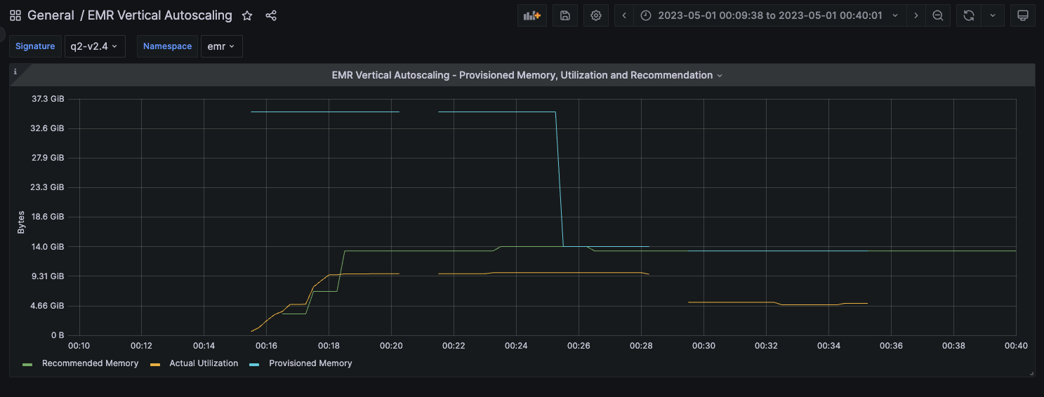
Results are presented categorized by your Kubernetes namespace and job signature. When you choose a certain namespace and signature combination, you’re presented with a pane. The pane represents a comparison of the vertical autoscaling recommendations for jobs belonging to the chosen signature, compared to the actual resource utilization of that job and the amount of Spark executor memory provisioned to the job. If autoscaling is enabled, the expectation is that the Spark executor memory would track the recommendation. If you’re in monitoring mode however, the two won’t match but you can still view the recommendations from this dashboard or use them to better understand the actual utilization and resource profile of your job.
Illustration of provisioned memory, utilization and recommendations
To better illustrate vertical autoscaling behavior and usage for different workloads, we executed query 2 of the TPC-DS benchmark for 5 iterations — The first two iterations in monitoring mode and the last 3 in autoscaling mode and visualized the results in the Grafana dashboard shared in the previous section.
Monitoring mode
This particular job was provisioned to run with 32GB of executor memory (the blue line in the image) but the actual utilization hovered at around the 10 GB mark (amber line). Vertical autoscaling computes a recommendation of approximately 14 GB based on this run (the green line). This recommendation is based on the actual utilization with a safety margin added in.
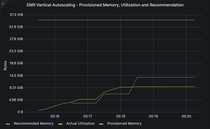
The second iteration of the job was also run in the monitoring mode and the utilization and the recommendations remained unchanged.

Autoscaling mode
Iterations 3 through 5 were run in autoscaling mode. In this case, the provisioned memory drops from 32GB to match the recommended value of 14GB (the blue line).
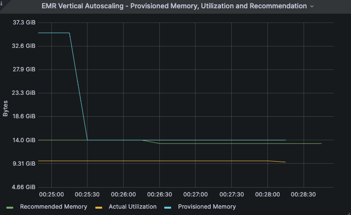
The utilization and recommendations remained unchanged for subsequent iterations in the case of this example. Furthermore, we observed that all the iterations of the job completed in around 5 minutes, both with and without autoscaling. This example illustrates the successful scaling down of the job’s executor memory allocation by about 56% (a drop from 32GB to approximately 14 GB) which also translates to an equivalent reduction in the EMR memory uplift costs of the job, with no impact to the job’s performance.
Automatic OOM recovery
In the earlier example, we didn’t observe any OOM events as a result of autoscaling. In the rare occasion where autoscaling results in OOM events, jobs should usually be scaled back up automatically. On the other hand, if a job that has autoscaling enabled is under-provisioned and as a result experiences OOM events, vertical autoscaling can scale up resources to facilitate automatic recovery.
In the following example, a job was provisioned with 2.5 GB of executor memory and experienced OOM exceptions during its execution. Vertical autoscaling responded to the OOM events by automatically scaling up failed executors when they were re-started. As seen in the following image, when the amber line representing memory utilization started approaching the blue line representing the provisioned memory, vertical autoscaling kicked in to increase the amount of provisioned memory for the re-started executors, allowing the automatic recovery and successful completion of the job without any intervention. The recommended memory converged to approximately 5 GB before the job completed.
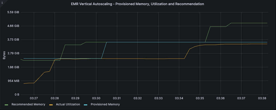
All subsequent runs of jobs with the same signature will now start-up with the recommended settings computed earlier, preventing OOM events right from the start.
Cleanup
Refer to documentation for information on cleaning up vertical autoscaling related resources from your cluster. To cleanup your EMR on EKS cluster after trying out the vertical autoscaling feature, refer to the clean-up section of the EMR on EKS workshop.
Conclusion
You can use vertical autoscaling to easily monitor resource utilization for one or more EMR on EKS jobs without any impact to your production workloads. You can use standard Kubernetes tooling including Prometheus, Grafana and kubectl to interact with and monitor vertical autoscaling on your cluster. You can also autoscale your EMR Spark jobs using recommendations that are derived based on the needs of your job, allowing you to realize cost savings and optimize cluster utilization as well as build resiliency to out-of-memory errors. Additionally, you can use it in conjunction with existing autoscaling mechanisms such as Dynamic Resource Allocation and Karpenter to effortlessly achieve optimal vertical resource assignment. Looking ahead, when Kubernetes fully supports in-place resizing of pods, vertical autoscaling will be able to take advantage of it to seamlessly scale your EMR jobs up or down, further facilitating optimal costs and cluster utilization.
To learn more about EMR on EKS vertical autoscaling and getting started with it, refer to documentation. You can also use the EMR on EKS Workshop to try out the EMR on EKS deployment option for Amazon EMR.
About the author
 Rajkishan Gunasekaran is a Principal Engineer for Amazon EMR on EKS at Amazon Web Services.
The Transparency in Coverage rule is a federal regulation in the United States that was finalized by the Center for Medicare and Medicaid Services (CMS) in October 2020. The rule requires health insurers to provide clear and concise information to consumers about their health plan benefits, including costs and coverage details. Under the rule, health insurers must make available to their members a list of negotiated rates for in-network providers, as well as an estimate of the member’s out-of-pocket costs for specific health care services. This information must be made available to members through an online tool that is accessible and easy to use. The Transparency in Coverage rule also requires insurers to make available data files that contain detailed information on the prices they negotiate with health care providers. This information can be used by employers, researchers, and others to compare prices across different insurers and health care providers. Phase 1 implementation of this regulation, which went into effect on July 1, 2022, requires that payors publish machine-readable files publicly for each plan that they offer. CMS (Center for Medicare and Medicaid Services) has published a technical implementation guide with file formats, file structure, and standards on producing these machine-readable files.
This post walks you through the preprocessing and processing steps required to prepare data published by health insurers in light of this federal regulation using AWS Glue. We also show how to query and derive insights using Amazon Athena.
AWS Glue is a serverless data integration service that makes it straightforward to discover, prepare, move, and integrate data from multiple sources for analytics, machine learning (ML), and application development. Athena is a serverless, interactive analytics service built on open-source frameworks, supporting open-table and file formats. Athena provides a simplified, flexible way to analyze petabytes of data.
Challenges processing these machine-readable files
The machine-readable files published by these payors vary in size. A single file can range from a few megabytes to hundreds of gigabytes. These files contain large JSON objects that are deeply nested. Unlike NDJSON and JSONL formats, where each line in the file is a JSON object, these files contain a single large JSON object that can span across multiple lines. The following figure represents the schema of an in\_network rate file published by a major health insurer on their website for public access. This file, when uncompressed, is about 20 GB in size, contains a single JSON object, and is deeply nested. The following figure represents the schema of this JSON object when printed using the Spark printSchema() function. Each highlighted box in red is a nested array structure.

Loading a 20 GB deeply nested JSON object requires a machine with a large memory footprint. Data when loaded into memory is 4–10 times its size on disk. A 20 GB JSON object may need a machine with up to 200 GB memory. To process workloads larger than 20 GB, these machines need to be scaled vertically, thereby significantly increasing hardware costs. Vertical scaling has its limits, and it’s not possible to scale beyond a certain point. Analyzing this data requires unnesting and flattening of deeply nested array structures. These transformations explode the data at an exponential rate, thereby adding to the need for more memory and disk space.
You can use an in-memory distributed processing framework such as Apache Spark to process and analyze such large volumes of data. However, to load this single large JSON object as a Spark DataFrame and perform an action on it, a worker node needs enough memory to load this object in full. When a worker node tries to load this large deeply nested JSON object and there isn’t enough memory to load it in full, the processing job will fail with out-of-memory issues. This calls for splitting the large JSON object into smaller chunks using some form of preprocessing logic. Once preprocessed, these smaller files can then be further processed in parallel by worker nodes without running into out-of-memory issues.
Solution overview
The solution involves a two-step approach. The first is a preprocessing step, which takes the large JSON object as input and splits it to multiple manageable chunks. This is required to address the challenges we mentioned earlier. The second is a processing step, which prepares and publishes data for analysis.
The preprocessing step uses an AWS Glue Python shell job to split the large JSON object into smaller JSON files. The processing step unnests and flattens the array items from these smaller JSON files in parallel. It then partitions and writes the output as Parquet on Amazon Simple Storage Service (Amazon S3). The partitioned data is cataloged and analyzed using Athena. The following diagram illustrates this workflow.

Prerequisites
To implement the solution in your own AWS account, you need to create or configure the following AWS resources in advance:
- An S3 bucket to persist the source and processed data. Download the input file and upload it to the path
s3://yourbucket/ptd/2023-03-01\_United-HealthCare-Services—Inc-\_Third-Party-Administrator\_PS1-50\_C2\_in-network-rates.json.gz. - An AWS Identity and Access Management (IAM) role for your AWS Glue extract, transform, and load (ETL) job. For instructions, refer to Setting up IAM permissions for AWS Glue. Adjust the permissions to ensure AWS Glue has read/write access to Amazon S3 locations.
- An IAM role for Athena with AWS Glue Data Catalog permissions to create and query tables.
Create an AWS Glue preprocessing job
The preprocessing step uses ijson, an open-source iterative JSON parser to extract items in the outermost array of top-level attributes. By streaming and iteratively parsing the large JSON file, the preprocessing step loads only a portion of the file into memory, thereby avoiding out-of-memory issues. It also uses s3pathlib, an open-source Python interface to Amazon S3. This makes it easy to work with S3 file systems.
To create and run the AWS Glue job for preprocessing, complete the following steps:
- On the AWS Glue console, choose Jobs under Glue Studio in the navigation pane.
- Create a new job.
- Select Python shell script editor.
- Select Create a new script with boilerplate code.

- Enter the following code into the editor (adjust the S3 bucket names and paths to point to the input and output locations in Amazon S3):
- Update the properties of your job on the Job details tab:
- For Type, choose Python Shell.
- For Python version, choose Python 3.9.
- For Data processing units, choose 1 DPU.
For Python shell jobs, you can allocate either 0.0625 or 1 DPU. The default is 0.0625 DPU. A DPU is a relative measure of processing power that consists of 4 vCPUs of compute capacity and 16 GB of memory.

The Python libraries ijson and s3pathlib are available in pip and can be installed using the AWS Glue job parameter --additional-python-modules. You can also choose to package these libraries, upload them to Amazon S3, and refer to them from your AWS Glue job. For instructions on packaging your library, refer to Providing your own Python library.
- To install the Python libraries, set the following job parameters:
- Key –
--additional-python-modules - Value –
ijson,s3pathlib
- Key –
- Run the job.
The preprocessing step creates three folders in the S3 bucket: base, in\_network and provider\_references.

Files in in\_network and provider\_references folders contains array of JSON objects. Each of these JSON objects represents an element in the outermost array of the original large JSON object.

Create an AWS Glue processing job
The processing job uses the output of the preprocessing step to create a denormalized view of data by extracting and flattening elements and attributes from nested arrays. The extent of unnesting depends on the attributes we need for analysis. For example, attributes such as negotiated\_rate, npi, and billing\_code are essential for analysis and extracting values associated with these attributes requires multiple levels of unnesting. The denormalized data is then partitioned by the billing\_code column, persisted as Parquet on Amazon S3, and registered as a table on the AWS Glue Data Catalog for querying.
The following code sample guides you through the implementation using PySpark. The columns used to partition the data depends on query patterns used to analyze the data. Arriving at a partitioning strategy that is in line with the query patterns will improve overall query performance during analysis. This post assumes that the queries used for analyzing data will always use the column billing\_code to filter and fetch data of interest. Data in each partition is bucketed by npi to improve query performance.
To create your AWS Glue job, complete the following steps:
- On the AWS Glue console, choose Jobs under Glue Studio in the navigation pane.
- Create a new job.
- Select Spark script editor.
- Select Create a new script with boilerplate code.
- Enter the following code into the editor (adjust the S3 bucket names and paths to point to the input and output locations in Amazon S3):
- Update the properties of your job on the Job details tab:
- For Type, choose Spark.
- For Glue version, choose Glue 4.0.
- For Language, choose Python 3.
- For Worker type, choose G 2X.
- For Requested number of workers, enter 20.
Arriving at the number of workers and worker type to use for your processing job depends on factors such as the amount of data being processed, the speed at which it needs to be processed, and the partitioning strategy used. Repartitioning of data can result in out-of-memory issues, especially when data is heavily skewed on the column used to repartition. It’s possible to reach Amazon S3 service limits if too many workers are assigned to the job. This is because tasks running on these worker nodes may try to read/write from the same S3 prefix, causing Amazon S3 to throttle the incoming requests. For more details, refer to Best practices design patterns: optimizing Amazon S3 performance.

Exploding array elements creates new rows and columns, thereby exponentially increasing the amount of data that needs to be processed. Apache Spark splits this data into multiple Spark partitions on different worker nodes so that it can process large amounts of data in parallel. In Apache Spark, shuffling happens when data needs to be redistributed across the cluster. Shuffle operations are commonly triggered by wide transformations such as join, reduceByKey, groupByKey, and repartition. In case of exceptions due to local storage limitations, it helps to supplement or replace local disk storage capacity with Amazon S3 for large shuffle operations. This is possible with the AWS Glue Spark shuffle plugin with Amazon S3. With the cloud shuffle storage plugin for Apache Spark, you can avoid disk space-related failures.
- To use the Spark shuffle plugin, set the following job parameters:
- Key –
--write-shuffle-files-to-s3 - Value –
true

- Key –
Query the data
You can query the cataloged data using Athena. For instructions on setting up Athena, refer to Setting up.
On the Athena console, choose Query editor in the navigation pane to run your query, and specify your data source and database.

To find the minimum, maximum, and average negotiated rates for procedure codes, run the following query:
The following screenshot shows the query results.

Clean up
To avoid incurring future charges, delete the AWS resources you created:
- Delete the S3 objects and bucket.
- Delete the IAM policies and roles.
- Delete the AWS Glue jobs for preprocessing and processing.
Conclusion
This post guided you through the necessary preprocessing and processing steps to query and analyze price transparency-related machine-readable files. Although it’s possible to use other AWS services to process such data, this post focused on preparing and publishing data using AWS Glue.
To learn more about the Transparency in Coverage rule, refer to Transparency in Coverage. For best practices for scaling Apache Spark jobs and partitioning data with AWS Glue, refer to Best practices to scale Apache Spark jobs and partition data with AWS Glue. To learn how to monitor AWS Glue jobs, refer to Monitoring AWS Glue Spark jobs.
We look forward to hearing any feedback or questions.
About the Authors
 Hari Thatavarthy is a Senior Solutions Architect on the AWS Data Lab team. He helps customers design and build solutions in the data and analytics space. He believes in data democratization and loves to solve complex data processing-related problems. In his spare time, he loves to play table tennis.
 Krishna Maddileti is a Senior Solutions Architect on the AWS Data Lab team. He partners with customers on their AWS journey and helps them with data engineering, data lakes, and analytics. In his spare time, he enjoys spending time with his family and playing video games with his 7-year-old.
 Yadukishore Tatavarthi is a Senior Partner Solutions Architect at AWS. He works closely with global system integrator partners to enable and support customers moving their workloads to AWS.
 Manish Kola is a Solutions Architect on the AWS Data Lab team. He partners with customers on their AWS journey.
 Noritaka Sekiyama is a Principal Big Data Architect on the AWS Glue team. He is responsible for building software artifacts to help customers. In his spare time, he enjoys cycling with his new road bike.
Customers use Amazon OpenSearch Service for mission-critical applications and monitoring. But what happens when OpenSearch Service itself is unavailable? If your ecommerce search is down, for example, you’re losing revenue. If you’re monitoring your application with OpenSearch Service, and it becomes unavailable, your ability to detect, diagnose, and repair issues with your application is diminished. In these cases, you may suffer lost revenue, customer dissatisfaction, reduced productivity, or even damage to your organization’s reputation.
OpenSearch Service offers an SLA of three 9s (99.9%) availability when following best practices. However, following those practices is complicated, and can require knowledge of and experience with OpenSearch’s data deployment and management, along with an understanding of how OpenSearch Service interacts with AWS Availability Zones and networking, distributed systems, OpenSearch’s self-healing capabilities, and its recovery methods. Furthermore, when an issue arises, such as a node becoming unresponsive, OpenSearch Service recovers by recreating the missing shards (data), causing a potentially large movement of data in the domain. This data movement increases resource usage on the cluster, which can impact performance. If the cluster is not sized properly, it can experience degraded availability, which defeats the purpose of provisioning the cluster across three Availability Zones.
Today, AWS is announcing the new deployment option Multi-AZ with Standby for OpenSearch Service, which helps you offload some of that heavy lifting in terms of high frequency monitoring, fast failure detection, and quick recovery from failure, and keeps your domains available and performant even in the event of an infrastructure failure. With Multi-AZ with Standby, you get 99.99% availability with consistent performance for a domain.
In this post, we discuss the benefits of this new option and how to configure your OpenSearch cluster with Multi-AZ with Standby.
Solution overview
The OpenSearch Service team has incorporated years of experience running tens of thousands of domains for our customers into the Multi-AZ with Standby feature. When you adopt Multi-AZ with Standby, OpenSearch Service creates a cluster across three Availability Zones, with each Availability Zone containing a complete copy of data in the cluster. OpenSearch Service then puts one Availability Zone into standby mode, routing all queries to the other two Availability Zones. When it detects a hardware-related failure, OpenSearch Service promotes nodes from the standby pool to become active in less than a minute. When you use Multi-AZ with Standby, OpenSearch Service doesn’t need to redistribute or recreate data from missing nodes. As a result, cluster performance is unaffected, removing the risk of degraded availability.
Prerequisites
Multi-AZ with Standby requires the following prerequisites:
- The domain needs to run on OpenSearch 1.3 or above
- The domain is deployed across three Availability Zones
- The domain has three (or a multiple of three) data notes
- You must use three dedicated cluster manager (master) nodes
Refer to Sizing Amazon OpenSearch Service domains for guidance on sizing your domain and dedicated cluster manager nodes.
Configure your OpenSearch cluster using Multi-AZ with Standby
You can use Multi-AZ with Standby when you create a new domain, or you can add it to an existing domain. If you’re creating a new domain using the AWS Management Console, you can create it with Multi-AZ with Standby by either selecting the new Easy create option or the traditional Standard create option. You can update existing domains to use Multi-AZ with Standby by editing their domain configuration.
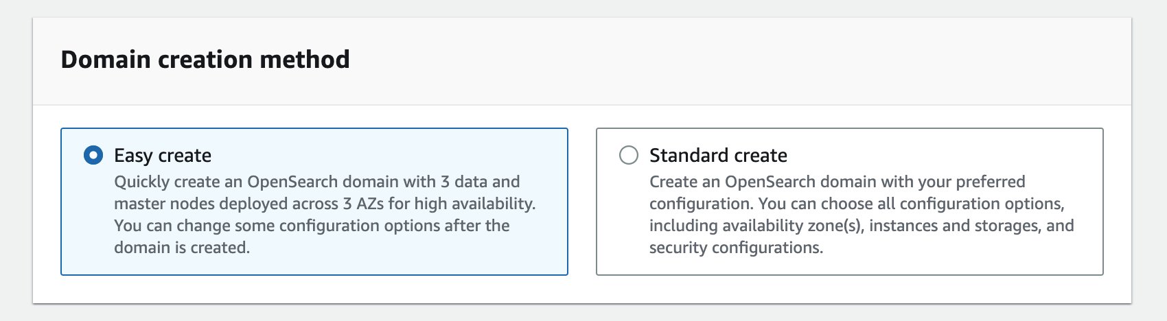
The Easy create option, as the name suggests, makes creating a domain easier by defaulting to best practice choices for most of the configuration (the majority of which can be altered later). The domain will be set up for high availability from the start and deployed as Multi-AZ with Standby.

While choosing the data nodes, you should choose three (or a multiple of three) data nodes so that they are equally distributed across each of the Availability Zones. The Data nodes table on the OpenSearch Service console provides a visual representation of the data notes, showing that one of the Availability Zones will be put on standby.

Similarly, while selecting the cluster manager (master) node, consider the number of data nodes, indexes, and shards that you plan to have before deciding the instance size.
After the domain is created, you can check its deployment type on the OpenSearch Service console under Cluster configuration, as shown in the following screenshot.

While creating an index, make sure that the number of copies (primary and replica) are multiples of three. If you don’t specify the number of replicas, the service will default to two. This is important so that there is at least one copy of the data in each Availability Zone. We recommend using an index template or similar for logs workloads.
OpenSearch Service distributes the nodes and data copies equally across the three Availability Zones. During normal operations, the standby nodes don’t receive any search requests. The two active Availability Zones respond to all the search requests. However, data is replicated to these standby nodes to ensure you have a full copy of the data in each Availability Zone at all times.
Response to infrastructure failure events
OpenSearch Service continuously monitors the domain for events like node failure, disk failure, or Availability Zone failure. In the event of an infrastructure failure like an Availability Zone failure, OpenSearch Services promotes the standby nodes to active while the impacted Availability Zone recovers. Impact (if any) is limited to the in-flight requests as traffic is weighed away from the impacted Availability Zone in less a minute.
You can check the status of the domain, data node metrics for both active and standby, and Availability Zone rotation metrics on the Cluster health tab. The following screenshots show the cluster health and metrics for data nodes such as CPU utilization, JVM memory pressure, and storage.


The following screenshot of the AZ Rotation Metrics section (you can find this under Cluster health tab) shows the read and write status of the Availability Zones. OpenSearch Service rotates the standby Availability Zone every 30 minutes to ensure the system is running and ready to respond to events. Availability Zones responding to traffic have a read value of 1, and the standby Availability Zone has a value of 0.
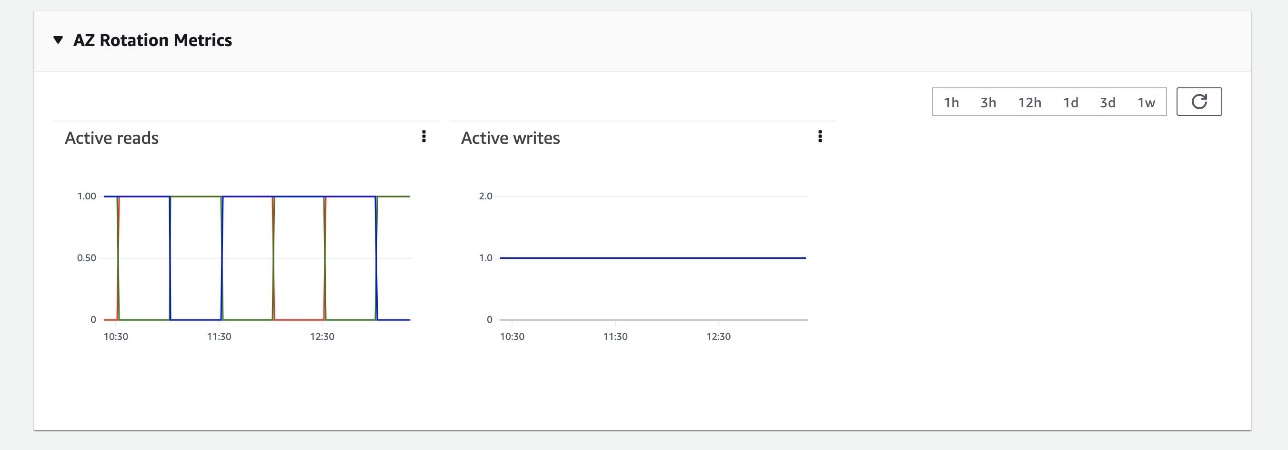
Considerations
Several improvements and guardrails have been made for this feature that offer higher availability and maintain performance. Some static limits have been applied that are specifically related to the number of shards per node, number of shards for a domain, and the size of a shard. OpenSearch Service also enables Auto-Tune by default. Multi-AZ with Standby restricts the storage to GP3- or SSD-backed instances for the most cost-effective and performant storage options. Additionally, we’re introducing an advanced traffic shaping mechanism that will detect rogue queries, which further enhances the reliability of the domain.
We recommend evaluating your domain infrastructure needs based on your workload to achieve high availability and performance.
Conclusion
Multi-AZ with Standby is now available on OpenSearch Service in all AWS Regions globally where OpenSearch service is available, except US West (N. California), and AWS GovCloud (US-Gov-East, US-Gov-West). Try it out and send your feedback to AWS re:Post for Amazon OpenSearch Service or through your usual AWS support contacts.
About the authors
Prashant Agrawal is a Sr. Search Specialist Solutions Architect with Amazon OpenSearch Service. He works closely with customers to help them migrate their workloads to the cloud and helps existing customers fine-tune their clusters to achieve better performance and save on cost. Before joining AWS, he helped various customers use OpenSearch and Elasticsearch for their search and log analytics use cases. When not working, you can find him traveling and exploring new places. In short, he likes doing Eat → Travel → Repeat.
Rohin Bhargava is a Sr. Product Manager with the Amazon OpenSearch Service team. His passion at AWS is to help customers find the correct mix of AWS services to achieve success for their business goals.
Today, we’re pleased to introduce the Amazon EMR CLI, a new command line tool to package and deploy PySpark projects across different Amazon EMR environments. With the introduction of the EMR CLI, you now have a simple way to not only deploy a wide range of PySpark projects to remote EMR environments, but also integrate with your CI/CD solution of choice.
In this post, we show how you can use the EMR CLI to create a new PySpark project from scratch and deploy it to Amazon EMR Serverless in one command.
Overview of solution
The EMR CLI is an open-source tool to help improve the developer experience of developing and deploying jobs on Amazon EMR. When you’re just getting started with Apache Spark, there are a variety of options with respect to how to package, deploy, and run jobs that can be overwhelming or require deep domain expertise. The EMR CLI provides simple commands for these actions that remove the guesswork from deploying Spark jobs. You can use it to create new projects or alongside existing PySpark projects.
In this post, we walk through creating a new PySpark project that analyzes weather data from the NOAA Global Surface Summary of Day open dataset. We’ll use the EMR CLI to do the following:
- Initialize the project.
- Package the dependencies.
- Deploy the code and dependencies to Amazon Simple Storage Service (Amazon S3).
- Run the job on EMR Serverless.
Prerequisites
For this walkthrough, you should have the following prerequisites:
- An AWS account
- An EMR Serverless application in the
us-east-1Region - An S3 bucket for your code and logs in the
us-east-1Region - An AWS Identity and Access Management (IAM) job role that can run EMR Serverless jobs and access S3 buckets
- Python version >= 3.7
- Docker
If you don’t already have an existing EMR Serverless application, you can use the following AWS CloudFormation template or use the emr bootstrap command after you’ve installed the CLI.
Install the EMR CLI
You can find the source for the EMR CLI in the GitHub repo, but it’s also distributed via PyPI. It requires Python version >= 3.7 to run and is tested on macOS, Linux, and Windows. To install the latest version, use the following command:
You should now be able to run the emr --help command and see the different subcommands you can use:
If you didn’t already create an EMR Serverless application, the bootstrap command can create a sample environment for you and a configuration file with the relevant settings. Assuming you used the provided CloudFormation stack, set the following environment variables using the information on the Outputs tab of your stack. Set the Region in the terminal to us-east-1 and set a few other environment variables we’ll need along the way:
We use us-east-1 because that’s where the NOAA GSOD data bucket is. EMR Serverless can access S3 buckets and other AWS resources in the same Region by default. To access other services, configure EMR Serverless with VPC access.
Initialize a project
Next, we use the emr init command to initialize a default PySpark project for us in the provided directory. The default templates create a standard Python project that uses pyproject.toml to define its dependencies. In this case, we use Pandas and PyArrow in our script, so those are already pre-populated.
After the project is initialized, you can run cd my-project or open the my-project directory in your code editor of choice. You should see the following set of files:
Note that we also have a Dockerfile here. This is used by the package command to ensure that our project dependencies are built on the right architecture and operating system for Amazon EMR.
If you use Poetry to manage your Python dependencies, you can also add a --project-type poetry flag to the emr init command to create a Poetry project.
If you already have an existing PySpark project, you can use emr init --dockerfile to create the Dockerfile necessary to package things up.
Run the project
Now that we’ve got our sample project created, we need to package our dependencies, deploy the code to Amazon S3, and start a job on EMR Serverless. With the EMR CLI, you can do all of that in one command. Make sure to run the command from the my-project directory:
This command performs several actions:
- Auto-detects the type of Spark project in the current directory.
- Initiates a build for your project to package up dependencies.
- Copies your entry point and resulting build files to Amazon S3.
- Starts an EMR Serverless job.
- Waits for the job to finish, exiting with an error status if it fails.
You should now see the following output in your terminal as the job begins running in EMR Serverless:
And that’s it! If you want to run the same code on Amazon EMR on Amazon Elastic Compute Cloud (Amazon EC2), you can replace --application-id with --cluster-id j-11111111. The CLI will take care of sending the right spark-submit commands to your EMR cluster.
Now let’s walk through some of the other commands.
emr package
PySpark projects can be packaged in numerous ways, from a single .py file to a complex Poetry project with various dependencies. The EMR CLI can help consistently package your projects without having to worry about the details.
For example, if you have a single .py file in your project directory, the package command doesn’t need to do anything. If, however, you have multiple .py files in a typical Python project style, the emr package command will zip these files up as a package that can later be uploaded to Amazon S3 and provided to your PySpark job using the --py-files option. If you have third party dependencies defined in pyproject.toml, emr package will create a virtual environment archive and start your EMR job with the spark.archive option.
The EMR CLI also supports Poetry for dependency management and packaging. If you have a Poetry project with a corresponding poetry.lock file, there’s nothing else you need to do. The emr package command will detect your poetry.lock file and automatically build the project using the Poetry Bundle plugin. You can use a Poetry project in two ways:
- Create a project using the
emr initcommand. The commands take a--project-typepoetry option that create a Poetry project for you: - If you have a pre-existing project, you can use the
emr init --dockerfileoption, which creates a Dockerfile that is automatically used when you runemr package.
Finally, as noted earlier, the EMR CLI provides you a default Dockerfile based on Amazon Linux 2 that you can use to reliably build package artifacts that are compatible with different EMR environments.
emr deploy
The emr deploy command takes care of copying the necessary artifacts for your project to Amazon S3, so you don’t have to worry about it. Regardless of how the project is packaged, emr deploy will copy the resulting files to your Amazon S3 location of choice.
One use case for this is with CI/CD pipelines. Sometimes you want to deploy a specific version of code to Amazon S3 to be used in your data pipelines. With emr deploy, this is as simple as changing the --s3-code-uri parameter.
For example, let’s assume you’ve already packaged your project using the emr package command. Most CI/CD pipelines allow you to access the git tag. You can use that as part of the emr deploy command to deploy a new version of your artifacts. In GitHub actions, this is github.ref\_name, and you can use this in an action to deploy a versioned artifact to Amazon S3. See the following code:
In your downstream jobs, you could then update the location of your entry point files to point to this new location when you’re ready, or you can use the emr run command discussed in the next section.
emr run
Let’s take a quick look at the emr run command. We’ve used it before to package, deploy, and run in one command, but you can also use it to run on already-deployed artifacts. Let’s look at the specific options:
If you want to run your code on EMR Serverless, the emr run command takes an --application-id and --job-role parameters. If you want to run on EMR on EC2, you only need the --cluster-id option.
Required for both options are --entry-point and --s3-code-uri. --entry-point is the main script that will be called by Amazon EMR. If you have any dependencies, --s3-code-uri is where they get uploaded to using the emr deploy command, and the EMR CLI will build the relevant spark-submit properties pointing to these artifacts.
There are a few different ways to customize the job:
- –job-name – Allows you to specify the job or step name
- –job-args – Allows you to provide command line arguments to your script
- –spark-submit-opts – Allows you to add additional
spark-submitoptions like--conf spark.jarsor others - –show-stdout – Currently only works with single-file .py jobs on EMR on EC2, but will display
stdoutin your terminal after the job is complete
As we’ve seen before, --build invokes both the package and deploy commands. This makes it easier to iterate on local development when your code still needs to run remotely. You can simply use the same emr run command over and over again to build, deploy, and run your code in your environment of choice.
Future updates
The EMR CLI is under active development. Updates are currently in progress to support Amazon EMR on EKS and allow for the creation of local development environments to make local iteration of Spark jobs even easier. Feel free to contribute to the project in the GitHub repository.
Clean up
To avoid incurring future charges, stop or delete your EMR Serverless application. If you used the CloudFormation template, be sure to delete your stack.
Conclusion
With the release of the EMR CLI, we’ve made it easier for you to deploy and run Spark jobs on EMR Serverless. The utility is available as open source on GitHub. We’re planning a host of new functionalities; if there are specific requests you have, feel free to file an issue or open a pull request!
About the author
 Damon is a Principal Developer Advocate on the EMR team at AWS. He’s worked with data and analytics pipelines for over 10 years and splits his team between splitting service logs and stacking firewood.
In today’s data-driven business environment, organizations face the challenge of efficiently preparing and transforming large amounts of data for analytics and data science purposes. Businesses need to build data warehouses and data lakes based on operational data. This is driven by the need to centralize and integrate data coming from disparate sources.
At the same time, operational data often originates from applications backed by legacy data stores. Modernizing applications requires a microservice architecture, which in turn necessitates the consolidation of data from multiple sources to construct an operational data store. Without modernization, legacy applications may incur increasing maintenance costs. Modernizing applications involves changing the underlying database engine to a modern document-based database like MongoDB.
These two tasks (building data lakes or data warehouses and application modernization) involve data movement, which uses an extract, transform, and load (ETL) process. The ETL job is a key functionality to having a well-structured process in order to succeed.
AWS Glue is a serverless data integration service that makes it straightforward to discover, prepare, move, and integrate data from multiple sources for analytics, machine learning (ML), and application development. MongoDB Atlas is an integrated suite of cloud database and data services that combines transactional processing, relevance-based search, real-time analytics, and mobile-to-cloud data synchronization in an elegant and integrated architecture.
By using AWS Glue with MongoDB Atlas, organizations can streamline their ETL processes. With its fully managed, scalable, and secure database solution, MongoDB Atlas provides a flexible and reliable environment for storing and managing operational data. Together, AWS Glue ETL and MongoDB Atlas are a powerful solution for organizations looking to optimize how they build data lakes and data warehouses, and to modernize their applications, in order to improve business performance, reduce costs, and drive growth and success.
In this post, we demonstrate how to migrate data from Amazon Simple Storage Service (Amazon S3) buckets to MongoDB Atlas using AWS Glue ETL, and how to extract data from MongoDB Atlas into an Amazon S3-based data lake.
Solution overview
In this post, we explore the following use cases:
- Extracting data from MongoDB – MongoDB is a popular database used by thousands of customers to store application data at scale. Enterprise customers can centralize and integrate data coming from multiple data stores by building data lakes and data warehouses. This process involves extracting data from the operational data stores. When the data is in one place, customers can quickly use it for business intelligence needs or for ML.
- Ingesting data into MongoDB – MongoDB also serves as a no-SQL database to store application data and build operational data stores. Modernizing applications often involves migration of the operational store to MongoDB. Customers would need to extract existing data from relational databases or from flat files. Mobile and web apps often require data engineers to build data pipelines to create a single view of data in Atlas while ingesting data from multiple siloed sources. During this migration, they would need to join different databases to create documents. This complex join operation would need significant, one-time compute power. Developers would also need to build this quickly to migrate the data.
AWS Glue comes handy in these cases with the pay-as-you-go model and its ability to run complex transformations across huge datasets. Developers can use AWS Glue Studio to efficiently create such data pipelines.
The following diagram shows the data extraction workflow from MongoDB Atlas into an S3 bucket using the AWS Glue Studio.
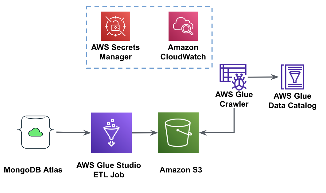
In order to implement this architecture, you will need a MongoDB Atlas cluster, an S3 bucket, and an AWS Identity and Access Management (IAM) role for AWS Glue. To configure these resources, refer to the prerequisite steps in the following GitHub repo.
The following figure shows the data load workflow from an S3 bucket into MongoDB Atlas using AWS Glue.

The same prerequisites are needed here: an S3 bucket, IAM role, and a MongoDB Atlas cluster.
Load data from Amazon S3 to MongoDB Atlas using AWS Glue
The following steps describe how to load data from the S3 bucket into MongoDB Atlas using an AWS Glue job. The extraction process from MongoDB Atlas to Amazon S3 is very similar, with the exception of the script being used. We call out the differences between the two processes.
- Create a free cluster in MongoDB Atlas.
- Upload the sample JSON file to your S3 bucket.
- Create a new AWS Glue Studio job with the Spark script editor option.

- Depending on whether you want to load or extract data from the MongoDB Atlas cluster, enter the load script or extract script in the AWS Glue Studio script editor.
The following screenshot shows a code snippet for loading data into the MongoDB Atlas cluster.
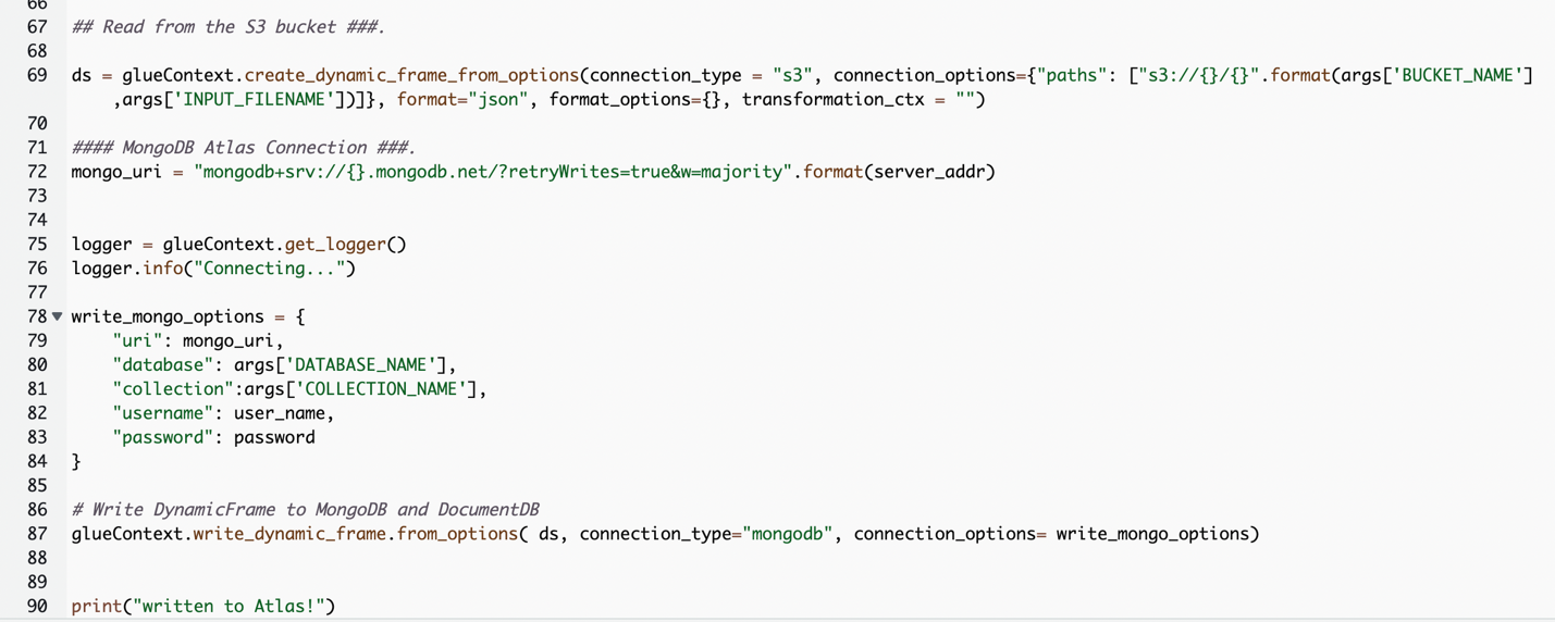
The code uses AWS Secrets Manager to retrieve the MongoDB Atlas cluster name, user name, and password. Then, it creates a DynamicFrame for the S3 bucket and file name passed to the script as parameters. The code retrieves the database and collection names from the job parameters configuration. Finally, the code writes the DynamicFrame to the MongoDB Atlas cluster using the retrieved parameters.
- Create an IAM role with the permissions as shown in the following screenshot.
For more details, refer to Configure an IAM role for your ETL job.
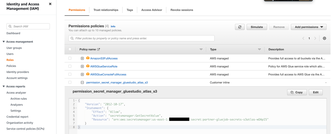
- Give the job a name and supply the IAM role created in the previous step on the Job details tab.
- You can leave the rest of the parameters as default, as shown in the following screenshots.


- Next, define the job parameters that the script uses and supply the default values.

- Save the job and run it.
- To confirm a successful run, observe the contents of the MongoDB Atlas database collection if loading the data, or the S3 bucket if you were performing an extract.


The following screenshot shows the results of a successful data load from an Amazon S3 bucket into the MongoDB Atlas cluster. The data is now available for queries in the MongoDB Atlas UI.
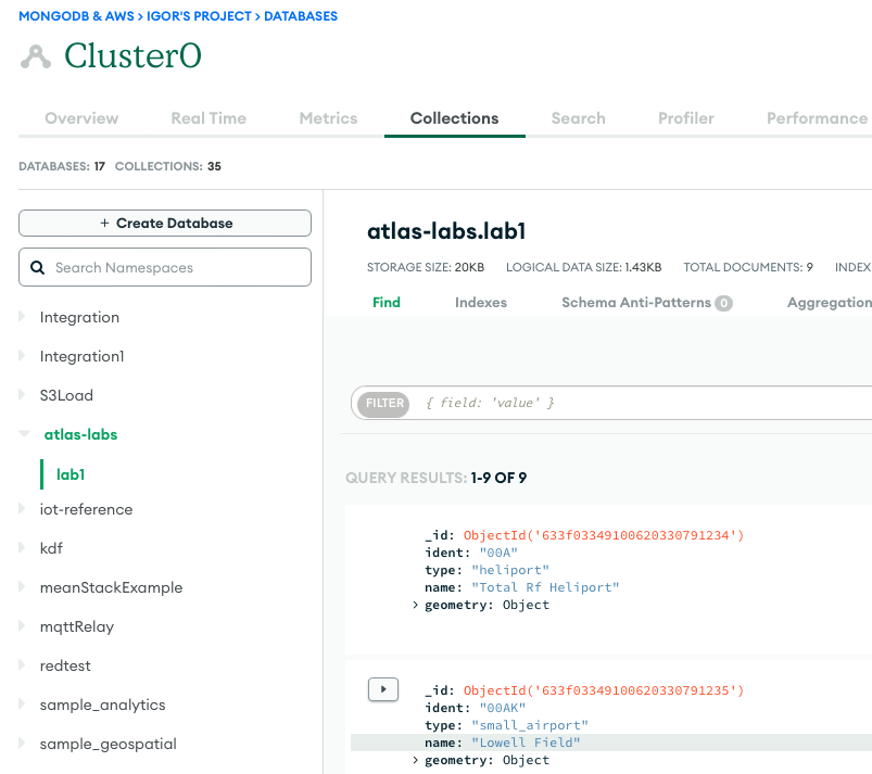
- To troubleshoot your runs, review the Amazon CloudWatch logs using the link on the job’s Run tab.
The following screenshot shows that the job ran successfully, with additional details such as links to the CloudWatch logs.

Conclusion
In this post, we described how to extract and ingest data to MongoDB Atlas using AWS Glue.
With AWS Glue ETL jobs, we can now transfer the data from MongoDB Atlas to AWS Glue-compatible sources, and vice versa. You can also extend the solution to build analytics using AWS AI and ML services.
To learn more, refer to the GitHub repository for step-by-step instructions and sample code. You can procure MongoDB Atlas on AWS Marketplace.
About the Authors

Igor Alekseev is a Senior Partner Solution Architect at AWS in Data and Analytics domain. In his role Igor is working with strategic partners helping them build complex, AWS-optimized architectures. Prior joining AWS, as a Data/Solution Architect he implemented many projects in Big Data domain, including several data lakes in Hadoop ecosystem. As a Data Engineer he was involved in applying AI/ML to fraud detection and office automation.
 Babu Srinivasan is a Senior Partner Solutions Architect at MongoDB. In his current role, he is working with AWS to build the technical integrations and reference architectures for the AWS and MongoDB solutions. He has more than two decades of experience in Database and Cloud technologies . He is passionate about providing technical solutions to customers working with multiple Global System Integrators(GSIs) across multiple geographies.
This is a guest blog post co-written with SangSu Park and JaeHong Ahn from SOCAR.
As companies continue to expand their digital footprint, the importance of real-time data processing and analysis cannot be overstated. The ability to quickly measure and draw insights from data is critical in today’s business landscape, where rapid decision-making is key. With this capability, businesses can stay ahead of the curve and develop new initiatives that drive success.
This post is a continuation of How SOCAR built a streaming data pipeline to process IoT data for real-time analytics and control. In this post, we provide a detailed overview of streaming messages with Amazon Managed Streaming for Apache Kafka (Amazon MSK) and Amazon ElastiCache for Redis, covering technical aspects and design considerations that are essential for achieving optimal results.
SOCAR is the leading Korean mobility company with strong competitiveness in car-sharing. SOCAR wanted to design and build a solution for a new Fleet Management System (FMS). This system involves the collection, processing, storage, and analysis of Internet of Things (IoT) streaming data from various vehicle devices, as well as historical operational data such as location, speed, fuel level, and component status.
This post demonstrates a solution for SOCAR’s production application that allows them to load streaming data from Amazon MSK into ElastiCache for Redis, optimizing the speed and efficiency of their data processing pipeline. We also discuss the key features, considerations, and design of the solution.
Background
SOCAR operates about 20,000 cars and is planning to include other large vehicle types such as commercial vehicles and courier trucks. SOCAR has deployed in-car devices that capture data using AWS IoT Core. This data was then stored in Amazon Relational Database Service (Amazon RDS). The challenge with this approach included inefficient performance and high resource usage. Therefore, SOCAR looked for purpose-built databases tailored to the needs of their application and usage patterns while meeting the future requirements of SOCAR’s business and technical requirements. The key requirements for SOCAR included achieving maximum performance for real-time data analytics, which required storing data in an in-memory data store.
After careful consideration, ElastiCache for Redis was selected as the optimal solution due to its ability to handle complex data aggregation rules with ease. One of the challenges faced was loading data from Amazon MSK into the database, because there was no built-in Kafka connector and consumer available for this task. This post focuses on the development of a Kafka consumer application that was designed to tackle this challenge by enabling performant data loading from Amazon MSK to Redis.
Solution overview
Extracting valuable insights from streaming data can be a challenge for businesses with diverse use cases and workloads. That’s why SOCAR built a solution to seamlessly bring data from Amazon MSK into multiple purpose-built databases, while also empowering users to transform data as needed. With fully managed Apache Kafka, Amazon MSK provides a reliable and efficient platform for ingesting and processing real-time data.
The following figure shows an example of the data flow at SOCAR.
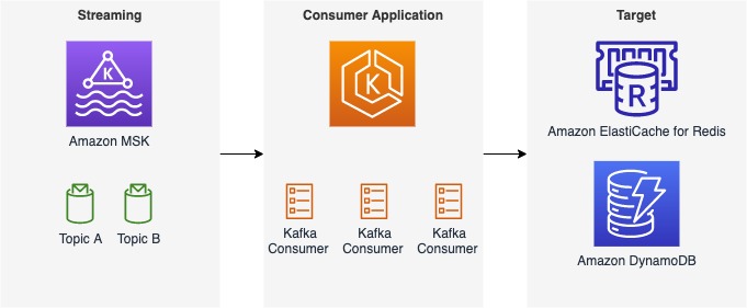
This architecture consists of three components:
- Streaming data – Amazon MSK serves as a scalable and reliable platform for streaming data, capable of receiving and storing messages from a variety of sources, including AWS IoT Core, with messages organized into multiple topics and partitions
- Consumer application – With a consumer application, users can seamlessly bring data from Amazon MSK into a target database or data storage while also defining data transformation rules as needed
- Target databases – With the consumer application, the SOCAR team was able to load data from Amazon MSK into two separate databases, each serving a specific workload
Although this post focuses on a specific use case with ElastiCache for Redis as the target database and a single topic called gps, the consumer application we describe can handle additional topics and messages, as well as different streaming sources and target databases such as Amazon DynamoDB. Our post covers the most important aspects of the consumer application, including its features and components, design considerations, and a detailed guide to the code implementation.
Components of the consumer application
The consumer application comprises three main parts that work together to consume, transform, and load messages from Amazon MSK into a target database. The following diagram shows an example of data transformations in the handler component.

The details of each component are as follows:
- Consumer – This consumes messages from Amazon MSK and then forwards the messages to a downstream handler.
- Loader – This is where users specify a target database. For example, SOCAR’s target databases include ElastiCache for Redis and DynamoDB.
- Handler – This is where users can apply data transformation rules to the incoming messages before loading them into a target database.
Features of the consumer application
This connection has three features:
- Scalability – This solution is designed to be scalable, ensuring that the consumer application can handle an increasing volume of data and accommodate additional applications in the future. For instance, SOCAR sought to develop a solution capable of handling not only the current data from approximately 20,000 vehicles but also a larger volume of messages as the business and data continue to grow rapidly.
- Performance – With this consumer application, users can achieve consistent performance, even as the volume of source messages and target databases increases. The application supports multithreading, allowing for concurrent data processing, and can handle unexpected spikes in data volume by easily increasing compute resources.
- Flexibility – This consumer application can be reused for any new topics without having to build the entire consumer application again. The consumer application can be used to ingest new messages with different configuration values in the handler. SOCAR deployed multiple handlers to ingest many different messages. Also, this consumer application allows users to add additional target locations. For example, SOCAR initially developed a solution for ElastiCache for Redis and then replicated the consumer application for DynamoDB.
Design considerations of the consumer application
Note the following design considerations for the consumer application:
- Scale out – A key design principle of this solution is scalability. To achieve this, the consumer application runs with Amazon Elastic Kubernetes Service (Amazon EKS) because it can allow users to increase and replicate consumer applications easily.
- Consumption patterns – To receive, store, and consume data efficiently, it’s important to design Kafka topics depending on messages and consumption patterns. Depending on messages consumed at the end, messages can be received into multiple topics of different schemas. For example, SOCAR has many different topics that are consumed by different workloads.
- Purpose-built database – The consumer application supports loading data into multiple target options based on the specific use case. For example, SOCAR stored real-time IoT data in ElastiCache for Redis to power real-time dashboard and web applications, while storing recent trip information in DynamoDB that didn’t require real-time processing.
Walkthrough overview
The producer of this solution is AWS IoT Core, which sends out messages into a topic called gps. The target database of this solution is ElastiCache for Redis. ElastiCache for Redis a fast in-memory data store that provides sub-millisecond latency to power internet-scale, real-time applications. Built on open-source Redis and compatible with the Redis APIs, ElastiCache for Redis combines the speed, simplicity, and versatility of open-source Redis with the manageability, security, and scalability from Amazon to power the most demanding real-time applications.
The target location can be either another database or storage depending on the use case and workload. SOCAR uses Amazon EKS to operate the containerized solution to achieve scalability, performance, and flexibility. Amazon EKS is a managed Kubernetes service to run Kubernetes in the AWS Cloud. Amazon EKS automatically manages the availability and scalability of the Kubernetes control plane nodes responsible for scheduling containers, managing application availability, storing cluster data, and other key tasks.
For the programming language, the SOCAR team decided to use the Go Programming language, utilizing both the AWS SDK for Go and a Goroutine, a lightweight logical or virtual thread managed by the Go runtime, which makes it easy to manage multiple threads. The AWS SDK for Go simplifies the use of AWS services by providing a set of libraries that are consistent and familiar for Go developers.
In the following sections, we walk through the steps to implement the solution:
- Create a consumer.
- Create a loader.
- Create a handler.
- Build a consumer application with the consumer, loader, and handler.
- Deploy the consumer application.
Prerequisites
For this walkthrough, you should have the following:
- An AWS account
- An MSK cluster
- An EKS cluster or Amazon Elastic Compute Cloud (Amazon EC2) instance
- ElastiCache for Redis
- An AWS Identity and Access Management (IAM) user for Amazon MSK (for more information, refer to How Amazon MSK works with IAM)
- Go (programming language)
Create a consumer
In this example, we use a topic called gps, and the consumer includes a Kafka client that receives messages from the topic. SOCAR created a struct and built a consumer (called NewConsumer in the code) to make it extendable. With this approach, any additional parameters and rules can be added easily.
To authenticate with Amazon MSK, SOCAR uses IAM. Because SOCAR already uses IAM to authenticate other resources, such as Amazon EKS, it uses the same IAM role (aws\_msk\_iam\_v2) to authenticate clients for both Amazon MSK and Apache Kafka actions.
The following code creates the consumer:
Create a loader
The loader function, represented by the Loader struct, is responsible for loading messages to the target location, which in this case is ElastiCache for Redis. The NewLoader function initializes a new instance of the Loader struct with a logger and a Redis cluster client, which is used to communicate with the ElastiCache cluster. The redis.NewClusterClient object is initialized using the NewRedisClient function, which uses IAM to authenticate the client for Redis actions. This ensures secure and authorized access to the ElastiCache cluster. The Loader struct also contains the Close method to close the Kafka reader and free up resources.
The following code creates a loader:
Create a handler
A handler is used to include business rules and data transformation logic that prepares data before loading it into the target location. It acts as a bridge between a consumer and a loader. In this example, the topic name is cars.gps.json, and the message includes two keys, lng and lat, with data type Float64. The business logic can be defined in a function like handlerFuncGpsToRedis and then applied as follows:
Build a consumer application with the consumer, loader, and handler
Now you have created the consumer, loader, and handler. The next step is to build a consumer application using them. In a consumer application, you read messages from your stream with a consumer, transform them using a handler, and then load transformed messages into a target location with a loader. These three components are parameterized in a consumer application function such as the one shown in the following code:
Deploy the consumer application
To achieve maximum parallelism, SOCAR containerizes the consumer application and deploys it into multiple pods on Amazon EKS. Each consumer application contains a unique consumer, loader, and handler. For example, if you need to receive messages from a single topic with five partitions, you can deploy five identical consumer applications, each running in its own pod. Similarly, if you have two topics with three partitions each, you should deploy two consumer applications, resulting in a total of six pods. It’s a best practice to run one consumer application per topic, and the number of pods should match the number of partitions to enable concurrent message processing. The pod number can be specified in the Kubernetes deployment configuration
There are two stages in the Dockerfile. The first stage is the builder, which installs build tools and dependencies, and builds the application. The second stage is the runner, which uses a smaller base image (Alpine) and copies only the necessary files from the builder stage. It also sets the appropriate user permissions and runs the application. It’s also worth noting that the builder stage uses a specific version of the Golang image, while the runner stage uses a specific version of the Alpine image, both of which are considered to be lightweight and secure images.
The following code is an example of the Dockerfile:
Conclusion
In this post, we discussed SOCAR’s approach to building a consumer application that enables IoT real-time streaming from Amazon MSK to target locations such as ElastiCache for Redis. We hope you found this post informative and useful. Thank you for reading!
About the Authors
 SangSu Park is the Head of Operation Group at SOCAR. His passion is to keep learning, embrace challenges, and strive for mutual growth through communication. He loves to travel in search of new cities and places.
 JaeHong Ahn is a DevOps Engineer in SOCAR’s cloud infrastructure team. He is dedicated to promoting collaboration between developers and operators. He enjoys creating DevOps tools and is committed to using his coding abilities to help build a better world. He loves to cook delicious meals as a private chef for his wife.
 Younggu Yun works at AWS Data Lab in Korea. His role involves helping customers across the APAC region meet their business objectives and overcome technical challenges by providing prescriptive architectural guidance, sharing best practices, and building innovative solutions together.
Amazon Redshift is a fast, fully managed, petabyte-scale data warehouse service that makes it simple and cost-effective to analyze all your data efficiently and securely. Users such as data analysts, database developers, and data scientists use SQL to analyze their data in Amazon Redshift data warehouses. Amazon Redshift provides a web-based Query Editor V2 in addition to supporting connectivity via ODBC/JDBC or the Amazon Redshift Data API.
Amazon Redshift Query Editor V2 makes it easy to query your data using SQL and gain insights by visualizing your results using charts and graphs with a few clicks. With Query Editor V2, you can collaborate with team members by easily sharing saved queries, results, and analyses in a secure way.
Analysts performing ad hoc analyses in their workspace need to load sample data in Amazon Redshift by creating a table and load data from desktop. They want to join that data with the curated data in their data warehouse. Data engineers and data scientists have test data, and want to load data into Amazon Redshift for their machine learning (ML) or analytics use cases.
In this post, we walk through a new feature in Query Editor V2 to easily load data files either from your local desktop or Amazon Simple Storage Service (Amazon S3).
Prerequisites
Complete the following prerequisite steps:
-
- Create an Amazon Redshift provisioned cluster or Serverless endpoint.
- Provide access to Query Editor V2 for your end-users. To enable your users to access Query Editor V2 using IAM, as an administrator, you can attach one of the following AWS-managed policies to the AWS Identity and Access Management (IAM) user or role to grant permission:
- AmazonRedshiftQueryEditorV2FullAccess – Grants full access to the Query Editor V2 operations and resources.
- AmazonRedshiftQueryEditorV2NoSharing – Grants the ability to work with Query Editor V2 without sharing resources.
- AmazonRedshiftQueryEditorV2ReadSharing – Grants the ability to work with Query Editor V2 with limited sharing of resources. The granted principal can read the resources shared with its team but can’t update them.
- AmazonRedshiftQueryEditorV2ReadWriteSharing – Grants the ability to work with Query Editor V2 with sharing of resources. The granted principal can read and update the resources shared with its team.
- Provide access to the S3 bucket to load data from a local desktop file.
- To enable your users to load data from a local desktop using Query Editor V2, as an administrator, you have to specify a common S3 bucket, and the user account must be configured with proper permissions. You can use the following IAM policy as an example to configure your IAM user or role:
- It’s also recommended to have proper separation of data access when loading data files from your local desktop. You can use the following S3 bucket policy as an example to separate data access between users of the staging bucket you configured:
Configure Query Editor V2 for your AWS account
As an admin, you must first configure Query Editor V2 before providing access to your end-users. On the Amazon Redshift console, choose Query editor v2 in the navigation pane.

If you’re accessing Query Editor v2 for the first time, you must configure your account by providing AWS Key Management Service (AWS KMS) encryption and, optionally, an S3 bucket.
By default, an AWS-owned key is used to encrypt resources. Optionally, you can create a symmetric customer managed key to encrypt Query Editor V2 resources such as saved queries and query results using the AWS KMS console or AWS KMS API operations.
The S3 bucket URI is required when loading data from your local desktop. You can provide the S3 URI of the same bucket that you configured earlier as a prerequisite.

If you have previously configured Query Editor V2 with only AWS KMS encryption, you can choose Account Settings after launching the interface to update the S3 URI to support loading from your local desktop.

Load data from your local desktop
Users such as data analysts, database developers, and data scientists can now load local files up to 5 MB in size into Amazon Redshift tables from Query Editor V2, without using the COPY command. The supported data formats are CSV, JSON, DELIMITER, FIXEDWIDTH, SHAPEFILE, AVRO, PARQUET, and ORC. Complete the following steps:
-
-
- On the Amazon Redshift console, navigate to Query Editor V2.
- Click on Load data.

- Choose Load from local file and Browse to choose a local file. You can download the student\_info.csv file to use as an example.
- If your file has column headers as the first row, keep the default selection of Ignore header rows as
1to ignore first row. - If your file has date columns, choose Data conversion parameters.

- Select Date format, set it to
autoand choose Next.

- Choose Load new table to automatically infer the file schema.
- Specify the values for Cluster or workgroup, Database, Schema, and Table (for example,
Student\_info) to load data to. - Choose Create table.

-
A success message appears that the table was created. Now you can load data into the newly created table from a local file.
-
-
- Choose Load data.

- Choose Load data.
-
A message appears that the data load was successful.
-
-
- Query the
Student\_infotable to see the data.

- Query the
-
Load data from Amazon S3
You can easily load data from Amazon S3 into an Amazon Redshift table using Query Editor V2. Complete the following steps:
-
-
- On the Amazon Redshift console, launch Query Editor V2 and connect to your cluster.
- Browse to the database name (for example,
dev), thepublicschema, and expand Tables. - You can automatically infer the schema of a S3 file similar to Load from local file option shown above however for this demo, we will also show you how to load data to an existing table. Run the following
create tablescript to make a sample table (for this example,public.customer):
-
-
-
- Choose Load data.

- Choose Load from S3 bucket.
- For this post, we load data from the TPCH Sample data GitHub repo, so for the S3 URI, enter
s3://redshift-downloads/TPC-H/2.18/10GB/customer.tbl. - For S3 file location, choose
us-east-1. - For File format, choose
Delimiter. - For Delimiter character, enter
|.

- Choose Data conversion parameters, then select Time format and Date format as
auto. - Choose Back.
- Choose Load data.
-
Refer to Data conversion parameters for more details.
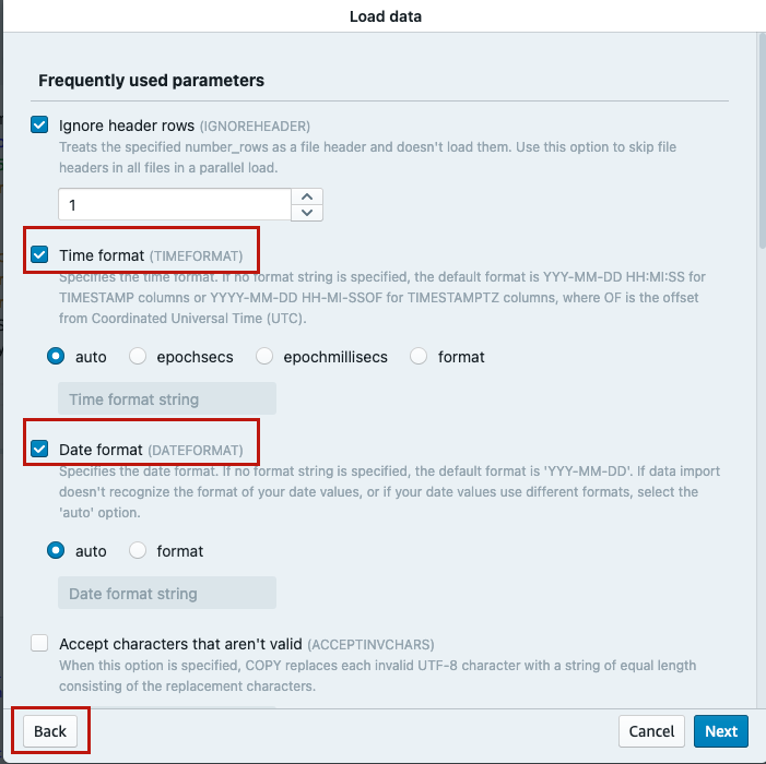
-
-
- Choose Load operations.
- Select Automatic update for compression encodings.
- Select Stop loading when maximum number of errors has been exceeded and specify a value (for example,
100). - Select Statistics update and ON, then choose Next.
-
Refer to Data load operations for more details.

-
-
- Choose Load existing table.
- Specify the Cluster or workgroup, Database, Schema (for example,
public) and Table name (for example,customer). - For IAM role, choose a suitable IAM role.
- Choose Load data.
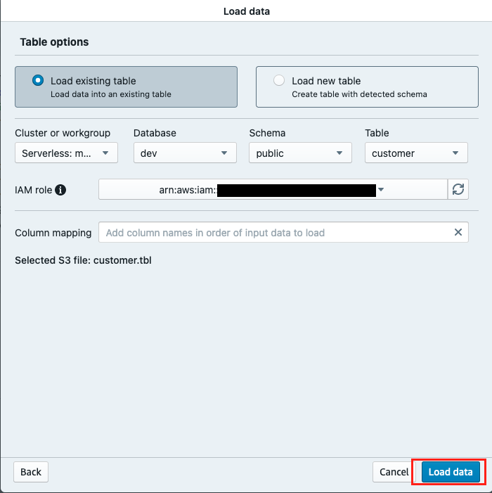
-
Query Editor V2 generates the COPY command and runs it on the Amazon Redshift cluster. The results of the COPY command are displayed in the Result section upon completion.

Conclusion
In this post, we showed how Amazon Redshift Query Editor V2 has simplified the process to load data into Amazon Redshift from Amazon S3 or your local desktop, thereby accelerating the data analysis. It’s an easy-to-use feature that your teams can start using to load and query datasets. If you have any questions or suggestions, please leave a comment.
About the Authors
 Raks Khare is an Analytics Specialist Solutions Architect at AWS based out of Pennsylvania. He helps customers architect data analytics solutions at scale on the AWS platform.
Tahir Aziz is an Analytics Solution Architect at AWS. He has worked with building data warehouses and big data solutions for over 13 years. He loves to help customers design end-to-end analytics solutions on AWS. Outside of work, he enjoys traveling and cooking.
 Erol Murtezaoglu, a Technical Product Manager at AWS, is an inquisitive and enthusiastic thinker with a drive for self-improvement and learning. He has a strong and proven technical background in software development and architecture, balanced with a drive to deliver commercially successful products. Erol highly values the process of understanding customer needs and problems, in order to deliver solutions that exceed expectations.
 Sapna Maheshwari is a Sr. Solutions Architect at Amazon Web Services. She has over 18 years of experience in data and analytics. She is passionate about telling stories with data and enjoys creating engaging visuals to unearth actionable insights.
 Karthik Ramanathan is a Software Engineer with Amazon Redshift and is based in San Francisco. He brings close to two decades of development experience across the networking, data storage and IoT verticals. When not at work he is also a writer and loves to be in the water.
 Albert Harkema is a Software Development Engineer at AWS. He is known for his curiosity and deep-seated desire to understand the inner workings of complex systems. His inquisitive nature drives him to develop software solutions that make life easier for others. Albert’s approach to problem-solving emphasizes efficiency, reliability, and long-term stability, ensuring that his work has a tangible impact. Through his professional experiences, he has discovered the potential of technology to improve everyday life.
Amazon Managed Workflows for Apache Airflow (Amazon MWAA) is a managed orchestration service for Apache Airflow that makes it simple to set up and operate end-to-end data pipelines in the cloud at scale. Amazon MWAA supports multiple versions of Apache Airflow (v1.10.12, v2.0.2, and v2.2.2). Earlier in 2023, we added support for Apache Airflow v2.4.3 so you can enjoy the same scalability, availability, security, and ease of management with Airflow’s most recent improvements. Additionally, with Apache Airflow v2.4.3 support, Amazon MWAA has upgraded to Python v3.10.8, which supports newer Python libraries like OpenSSL 1.1.1 as well as major new features and improvements.
In this post, we provide an overview of the features and capabilities of Apache Airflow v2.4.3 and how you can set up or upgrade your Amazon MWAA environment to accommodate Apache Airflow v2.4.3 as you orchestrate using workflows in the cloud at scale.
New feature: Data-aware scheduling using datasets
With the release of Apache Airflow v2.4.0, Airflow introduced datasets. An Airflow dataset is a stand-in for a logical grouping of data that can trigger a Directed Acyclic Graph (DAG) in addition to regular DAG triggering mechanisms such as cron expressions, timedelta objects, and Airflow timetables. The following are some of the attributes of a dataset:
- Datasets may be updated by upstream producer tasks, and updates to such datasets contribute to scheduling downstream consumer DAGs.
- You can create smaller, more self-contained DAGs, which chain together into a larger data-based workflow using datasets.
- You have an additional option now to create inter-DAG dependencies using datasets besides
ExternalTaskSensororTriggerDagRunOperator. You should consider using this dependency if you have two DAGs related via an irregular dataset update. This type of dependency also provides you with increased observability into the dependencies between your DAGs and datasets in the Airflow UI.
How data-aware scheduling works
You need to define three things:
- A dataset, or multiple datasets
- The tasks that will update the dataset
- The DAG that will be scheduled when one or more datasets are updated
The following diagram illustrates the workflow.

The producer DAG has a task that creates or updates the dataset defined by a Uniform Resource Identifier (URI). Airflow schedules the consumer DAG after the dataset has been updated. A dataset will be marked as updated only if the producer task completes successfully—if the task fails or if it’s skipped, no update occurs, and the consumer DAG will not be scheduled. If your updates to a dataset triggers multiple subsequent DAGs, then you can use the Airflow metric max\_active\_tasks\_per\_dag to control the parallelism of the consumer DAG and reduce the chance of overloading the system.
Let’s demonstrate this with a code example.
Prerequisites to build a data-aware scheduled DAG
You must have the following prerequisites:
- An Amazon Simple Storage Service (Amazon S3) bucket to upload datasets in. This can be a separate prefix in your existing S3 bucket configured for your Amazon MWAA environment, or it can be a completely different S3 bucket that you identify to store your data in.
- An Amazon MWAA environment configured with Apache Airflow v2.4.3. The Amazon MWAA execution role should have access to read and write to the S3 bucket configured to upload datasets. The latter is only needed if it’s a different bucket than the Amazon MWAA bucket.
The following diagram illustrates the solution architecture.

The workflow steps are as follows:
- The producer DAG makes an API call to a publicly hosted API to retrieve data.
- After the data has been retrieved, it’s stored in the S3 bucket.
- The update to this dataset subsequently triggers the consumer DAG.
You can access the producer and consumer code in the GitHub repo.
Test the feature
To test this feature, run the producer DAG. After it’s complete, verify that a file named test.csv is generated in the specified S3 folder. Verify in the Airflow UI that the consumer DAG has been triggered by updates to the dataset and that it runs to completion.
There are two restrictions on the dataset URI:
- It must be a valid URI, which means it must be composed of only ASCII characters
- The URI scheme can’t be an Airflow scheme (this is reserved for future use)
Other notable changes in Apache Airflow v2.4.3:
Apache Airflow v2.4.3 has the following additional changes:
- Deprecation of
schedule\_intervaland timetable arguments. Airflow v2.4.0 added a new DAG argument schedule that can accept a cron expression,timedeltaobject, timetable object, or list of dataset objects. - Removal of experimental Smart Sensors. Smart Sensors were added in v2.0 and were deprecated in favor of deferrable operators in v2.2, and have now been removed. Deferrable operators are not yet supported on Amazon MWAA, but will be offered in a future release.
- Implementation of
ExternalPythonOperatorthat can help you run some of your tasks with a different set of Python libraries than other tasks (and other than the main Airflow environment).
For detailed release documentation with sample code, visit the Apache Airflow v2.4.0 Release Notes.
New feature: Dynamic task mapping
Dynamic task mapping was a new feature introduced in Apache Airflow v2.3, which has also been extended in v2.4. Dynamic task mapping lets DAG authors create tasks dynamically based on current data. Previously, DAG authors needed to know how many tasks were needed in advance.
This is similar to defining your tasks in a loop, but instead of having the DAG file fetch the data and do that itself, the scheduler can do this based on the output of a previous task. Right before a mapped task is run, the scheduler will create n copies of the task, one for each input. The following diagram illustrates this workflow.

It’s also possible to have a task operate on the collected output of a mapped task, commonly known as map and reduce. This feature is particularly useful if you want to externally process various files, evaluate multiple machine learning models, or extraneously process a varied amount of data based on a SQL request.
How dynamic task mapping works
Let’s see an example using the reference code available in the Airflow documentation.
The following code results in a DAG with n+1 tasks, with n mapped invocations of count\_lines, each called to process line counts, and a total that is the sum of each of the count\_lines. Here n represents the number of input files uploaded to the S3 bucket.
With n=4 files uploaded, the resulting DAG would look like the following figure.

Prerequisites to build a dynamic task mapped DAG
You need the following prerequisites:
- An S3 bucket to upload files in. This can be a separate prefix in your existing S3 bucket configured for your Amazon MWAA environment, or it can be a completely different bucket that you identify to store your data in.
- An Amazon MWAA environment configured with Apache Airflow v2.4.3. The Amazon MWAA execution role should have access to read to the S3 bucket configured to upload files. The latter is only needed if it’s a different bucket than the Amazon MWAA bucket.
You can access the code in the GitHub repo.
Test the feature
Upload the four sample text files from the local data folder to an S3 bucket data folder. Run the dynamic\_task\_mapping DAG. When it’s complete, verify from the Airflow logs that the final sum is equal to the sum of the count lines of the individual files.
There are two limits that Airflow allows you to place on a task:
- The number of mapped task instances that can be created as the result of expansion
- The number of mapped tasks that can run at once
For detailed documentation with sample code, visit the Apache Airflow v2.3.0 Release Notes.
New feature: Upgraded Python version
With Apache Airflow v2.4.3 support, Amazon MWAA has upgraded to Python v3.10.8, providing support for newer Python libraries, features, and improvements. Python v3.10 has slots for data classes, match statements, clearer and better Union typing, parenthesized context managers, and structural pattern matching. Upgrading to Python v3.10 should also help you align with security standards by mitigating the risk of older versions of Python such as 3.7, which is fast approaching its end of security support.
With structural pattern matching in Python v3.10, you can now use switch-case statements instead of using if-else statements and dictionaries to simplify the code. Prior to Python v3.10, you might have used if statements, isinstance calls, exceptions and membership tests against objects, dictionaries, lists, tuples, and sets to verify that the structure of the data matches one or more patterns. The following code shows what an ad hoc pattern matching engine might have looked like prior to Python v3.10:
With structural pattern matching in Python v3.10, the code is as follows:
Python v3.10 also carries forward the performance improvements introduced in Python v3.9 using the vectorcall protocol. vectorcall makes many common function calls faster by minimizing or eliminating temporary objects created for the call. In Python 3.9, several Python built-ins—range, tuple, set, frozenset, list, dict—use vectorcall internally to speed up runs. The second big performance enhancer is more efficient in the parsing of Python source code using the new parser for the CPython runtime.
For a full list of Python v3.10 release highlights, refer to What’s New In Python 3.10.
The code is available in the GitHub repo.
Set up a new Apache Airflow v2.4.3 environment
You can set up a new Apache Airflow v2.4.3 environment in your account and preferred Region using either the AWS Management Console, API, or AWS Command Line Interface (AWS CLI). If you’re adopting infrastructure as code (IaC), you can automate the setup using either AWS CloudFormation, the AWS Cloud Development Kit (AWS CDK), or Terraform.
When you have successfully created an Apache Airflow v2.4.3 environment in Amazon MWAA, the following packages are automatically installed on the scheduler and worker nodes along with other provider packages:
apache-airflow-providers-amazon==6.0.0python==3.10.8
For a complete list of provider packages installed, refer to Apache Airflow provider packages installed on Amazon MWAA environments. Note that some imports and operator names have changed in the new provider package in order to standardize the naming convention across the provider package. For a complete list of provider package changes, refer to the package changelog.
Upgrade from Apache Airflow v2.0.2 or v2.2.2 to Apache Airflow v2.4.3
Currently, Amazon MWAA doesn’t support in-place upgrades of existing environments for older Apache Airflow versions. In this section, we show how you can transfer your data from your existing Apache Airflow v2.0.2 or v2.2.2 environment to Apache Airflow v2.4.3:
- Create a new Apache Airflow v2.4.3 environment.
- Copy your DAGs, custom plugins, and
requirements.txtresources from your existing v2.0.2 or v2.2.2 S3 bucket to the new environment’s S3 bucket.- If you use
requirements.txtin your environment, you need to update the--constraintto v2.4.3 constraints and verify that the current libraries and packages are compatible with Apache Airflow v2.4.3 - With Apache Airflow v2.4.3, the list of provider packages Amazon MWAA installs by default for your environment has changed. Note that some imports and operator names have changed in the new provider package in order to standardize the naming convention across the provider package. Compare the list of provider packages installed by default in Apache Airflow v2.2.2 or v2.0.2, and configure any additional packages you might need for your new v2.4.3 environment. It’s advised to use the aws-mwaa-local-runner utility to test out your new DAGs, requirements, plugins, and dependencies locally before deploying to Amazon MWAA.
- If you use
- Test your DAGs using the new Apache Airflow v2.4.3 environment.
- If you plan to migrate existing metadata from your previous environments to the new one, perform the export and import steps detailed in Migrating to a new Amazon MWAA environment.
- After you have confirmed that your tasks completed successfully, delete the v2.0.2 or v2.2.2 environment.
Conclusion
In this post, we talked about the new features of Apache Airflow v2.4.3 and how you can get started using it in Amazon MWAA. Try out these new features like data-aware scheduling, dynamic task mapping, and other enhancements along with Python v.3.10.
About the authors
Parnab Basak is a Solutions Architect and a Serverless Specialist at AWS. He specializes in creating new solutions that are cloud native using modern software development practices like serverless, DevOps, and analytics. Parnab works closely in the analytics and integration services space helping customers adopt AWS services for their workflow orchestration needs.
As organizations mature in their cloud journey, they have many accounts (even hundreds) that they need to manage. Imagine having to manage support cases for these accounts without a unified dashboard. Administrators have to access each account either by switching roles or with single sign-on (SSO) in order to view and manage support cases.
This post demonstrates how you can build an analytics pipeline to push support cases created in individual member AWS accounts into a central account. We also show you how to build an analytics dashboard to gain visibility and insights on all support cases created in various accounts within your organization.

Overview of solution
In this post, we go through the process to create a pipeline to ingest, store, process, analyze, and visualize AWS support cases. We use the following AWS services as key components:
- Amazon EventBridge and AWS Lambda to ingest support case data in real time from various AWS accounts
- Amazon Simple Storage Service (Amazon S3) to store the support case data
- AWS Glue DataBrew to clean and transform the data
- AWS Glue crawlers to catalog the data
- AWS Step Functions to orchestrate the flow
- Amazon Athena to query the processed data
- An Amazon QuickSight dashboard that provides insights into various support case metrics
The following diagram illustrates the architecture.

The central account is the AWS account that you use to centrally manage the support case data.
Member accounts are the AWS accounts where, whenever the support cases are created, the data flows into an S3 bucket in the central account that can be visualized using the QuickSight dashboard in the central account.
To implement this solution, you complete the following high-level steps:
- Determine the AWS accounts to use for the central account and member accounts.
- Set up permissions for AWS CloudFormation StackSets on the central account and member accounts.
- Create resources on the central account using AWS CloudFormation.
- Create resources on the member accounts using CloudFormation StackSets.
- Open up support cases on the member accounts.
- Visualize the data in a QuickSight dashboard in the central account.
Prerequisites
Complete the following prerequisite steps:
- Create AWS accounts if you haven’t done so already.
- Before you get started, make sure that you have a Business or Enterprise support plan for your member accounts.
- Sign up for QuickSight if you have never used QuickSight in this account before. To use the forecast capability in QuickSight, sign up for the Enterprise Edition.
Preparation for CloudFormation StackSets
In this section, we go through the steps to set up permissions for StackSets in both the central and member accounts.
Set up permissions for StackSets on the central account
To set up permissions on the central account, complete the following steps:
- Sign in to the AWS Management Console of the central account.
- Download the administrator role CloudFormation template.
- On the AWS CloudFormation console, choose Create stack and With new resources.
- Leave the Prepare template setting as default.
- For Template source, select Upload a template file.
- Choose Choose file and supply the CloudFormation template you downloaded:
AWSCloudFormationStackSetAdministrationRole.yml. - Choose Next.
- For Stack name, enter
StackSetAdministratorRole. - Choose Next.
- For Configure stack options, we recommend configuring tags, which are key-value pairs that can help you identify your stacks and the resources they create. For example, enter Owner as the key, and your email address as the value.
- We don’t use additional permissions or advanced options, so accept the default values and choose Next.
- Review your configuration and select I acknowledge that AWS CloudFormation might create IAM resources with custom names.
- Choose Create stack.
The stack takes about 30 seconds to complete.
Set up permissions for StackSets on member accounts
Now that we’ve created a StackSet administrator role on the central account, we need to create the StackSet execution role on the member accounts. Perform the following steps on all member accounts:
- Sign in to the console on the member account.
- Download the execution role CloudFormation template.
- On the AWS CloudFormation console, choose Create stack and With new resources.
- Leave the Prepare template setting as default.
- For Template source, select Upload a template file.
- Choose Choose file and supply the CloudFormation template you downloaded:
AWSCloudFormationStackSetExecutionRole.yml. - Choose Next.
- For Stack name, use
StackSetExecutionRole. - For Parameters, enter the 12-digit account ID for the central account.
- Choose Next.
- For Configure stack options, we recommend configuring tags. For example, enter Owner as the key and your email address as the value.
- We don’t use additional permissions or advanced options, so choose Next.
For more information, see Setting AWS CloudFormation stack options.
- Review your configuration and select I acknowledge that AWS CloudFormation might create IAM resources with custom names.
- Choose Create stack.
The stack takes about 30 seconds to complete.
Set up the infrastructure for the central account and member accounts
In this section, we go through the steps to create your resources for both accounts and launch the StackSets.
Create resources on the central account with AWS CloudFormation
To launch the provided CloudFormation template, complete the following steps:
- Sign in to the console on the central account.
- Choose Launch Stack:
- Choose Next.
- For Stack name, enter a name. For example,
support-case-central-account. - For AWSMemberAccountIDs, enter the member account IDs separated by commas from where support case data is gathered.
- For Support Case Raw Data Bucket, enter the S3 bucket in the central account that holds the support case raw data from all member accounts. Note the name of this bucket to use in future steps.
- For Support Case Transformed Data Bucket, enter the S3 bucket in central account that holds the support case transformed data. Note the name of this bucket to use in future steps.
- Choose Next.
- Enter any tags you want to assign to the stack and choose Next.
- Select the acknowledgement check boxes and choose Create stack.
The stack takes approximately 5 minutes to complete. Wait until the stack is complete before proceeding to the next steps.
Launch CloudFormation StackSets from the central account
To launch StackSets, complete the following steps:
- Sign in to the console on the central account.
- On the AWS CloudFormation console, choose StackSets in the navigation pane.
- Choose Create StackSet.
- Leave the IAM execution role name as
AWSCloudFormationStackSetExecutionRole. - If AWS Organizations is enabled, under permissions, select Service-managed permissions.
- Leave the Prepare template setting as default.
- For Template source, select Amazon S3 URL.
- Enter the following Amazon S3 URL under Specify Template:
https://aws-blogs-artifacts-public.s3.amazonaws.com/artifacts/BDB-2583/AWS\_MemberAccount\_SupportCaseDashboard\_CF.yaml - Choose Next.
- For StackSet name, enter a name. For example, support-case-member-account.
- For CentralSupportCaseRawBucket, enter the name of the Support Case Raw Data Bucket created in the central account, which you noted previously.
- For CentralAccountID, enter the account ID of the central account.
- For Configure StackSet options, we recommend configuring tags.
- Leave the rest as default and choose Next.
- If AWS Organizations is enabled, in the Set deployment options step, for Deployment targets, you can either choose Deploy to organization or Deploy to organizational units (OU).
- If you deploy to OUs, you will need to specify the AWS OU ID.
- If AWS Organizations is not enabled, on the Set Deployment Options page, under Accounts, select Deploy stacks in accounts.
- Under Account numbers, enter the 12-digit account IDs for the member accounts as a comma-separated list. For example: 111111111111,222222222222.
- Under Specify regions, choose US East (N. Virginia).
Due to the limitation of EventBridge with the AWS Support API, this StackSet has to be deployed only in the US East (N. Virginia) Region.
- Optionally, you can change the maximum concurrent accounts to match the number of member accounts, adjust the failure tolerance to at least 1, and choose Region Concurrency to be Parallel to set up resources in parallel on the member accounts.
- Review your selections, select the acknowledgement check boxes, and choose Submit.
The operation takes about 2–3 minutes to complete.
Visualize your support cases in QuickSight in the central account
In this section, we go through the steps to visualize your support cases in QuickSight.
Grant QuickSight permissions
To grant QuickSight permissions, complete the following steps:
- Sign in to the console on the central account.
- On the QuickSight console, on the Admin drop-down menu in top right-hand corner, choose Manage QuickSight.
- In the navigation pane, choose Security & permissions.
- Under QuickSight access to AWS services, choose Manage.
- Select Amazon Athena.
- Select Amazon S3 to edit QuickSight access to your S3 buckets.
- Select the bucket you specified during stack creation.
- Choose Finish.
- Choose Save.
Prepare the datasets
To prepare your datasets, complete the following steps:
- On the QuickSight console, choose Datasets in the navigation pane.
- Choose New dataset.
- Choose Athena.
- For Data source name, enter
support-case-data-source. - Choose Validate connection.
- After your connection is validated, choose Create data source.
- For Database, choose
support-case-transformed-data. - For Tables, select the table under the database (there should only be one table that matches the name of the S3 bucket you set as the destination for the transformed data).
- Choose Edit/Preview data.
- Leave Query mode set as Direct Query.
- Choose the options menu (three dots) next to the field
case\_creation\_yearand set Change data type to Date. - Enter the date format as
yyyy, then choose Validate and Update. - Similarly, right-click on the field
case\_creation\_monthand set Change data type to Date. - Enter the date format as
MM, then choose Validate and Update. - Right-click on the field
case\_creation\_dayand set Change data type to Date. - Enter the date format as
dd, then choose Validate and Update. - Right-click on the field
case\_creation\_timeand set Change data type to Date. - Enter the date format as
yyyy-MM-dd’T’HH:mm:ss.SSSZ, then choose Validate and Update. - Change the name of the QuickSight dataset to
support-cases-dataset. - Choose Save & publish.
- Note the dataset ID from the URL (alpha-numeric string between datasets and view, excluding slashes) to use later for QuickSight dashboard creation.

- Choose Cancel to exit this page.
Set up the QuickSight dashboard from a template
To set up your QuickSight dashboard, complete the following steps:
- Navigate to the following link, then right-click and choose Save As to download the QuickSight dashboard JSON template from the browser.
- On the console, choose the user profile drop-down menu.
- Choose the copy icon next to the Account ID: field (of the central account).

- Open the JSON file with a text editor and replace
xxxxxwith the account ID. This will be replaced in two places. - Replace
yyyyywith the dataset ID that you previously noted. - Replace
rrrrrwith the Region where you deployed resources in the central account.
To determine the principal (user) to be used for the dashboard creation, you can use AWS CloudShell.
- Navigate to CloudShell on the console. Ensure it’s the same Region where your resources are deployed.

- Wait until the environment gets created and you see the CloudShell prompt.

- Run the following command, providing your account ID (central account) and Region:
- From the output, select the value of the ARN field. Replace the value of
zzzzzwith the ARN. - Optionally, you can change the name of the dashboard by changing the value of the fields in the JSON file:
- For DashboardId, enter
SupportCaseCentralDashboard. - For Name, enter
SupportCaseCentralDashboard.
- For DashboardId, enter
- Save the changes to the JSON file.
Now we use CloudShell to upload the JSON file provided in the previous step.
- On the Actions menu, choose Upload file.

- To create the QuickSight dashboard from the JSON template, use the following AWS Command Line Interface (AWS CLI) command and pass the updated JSON file as an argument, providing your Region:
The output of the command looks similar to the following screenshot.

- In case of any issues or if you want to see more details about the dashboard, you can use the following command:
- On the QuickSight console, choose Dashboards in the navigation pane.
- Choose Support Cases Dashboard.
You should see a dashboard similar to the screenshot shown at the beginning of this post, but there should only be one case.
Add additional member accounts
If you want to add additional member accounts, you need to update the CloudFormation stack that you created earlier on the central account. If you followed our name recommendation, the stack is called support-case-central-account-stack. Add the additional account number in the Member Account IDs parameter.
Next, go to the StackSet in the central account. If you followed our naming recommendation, the StackSet is called support-case-member-account. Select the StackSet and on the Actions menu, choose Add stacks to StackSet. Then follow the same instructions that you followed previously when you created the StackSet.

Monitor support cases created in the central account
So far, our setup will monitor all support cases created in the member accounts that you specified. However, it doesn’t include support cases that you create in the central account. To set up monitoring for the central account, complete the following steps:
- Update the CloudFormation stack that you created earlier on the central account. If you followed our name recommendation, the stack is called support-case-central-account-stack. Add the central account ID in the Member Account IDs parameter.
- Sign in to the CloudFormation console in the central account.
- Choose Launch Stack:
- Choose Next.
- For Stack name, enter a name. For example,
support-case-central-as-member-account. - For CentralAccountIDs, enter the central account ID.
- For CentralSupportCaseRawBucket, enter the S3 bucket in the central account that holds the support case raw data from all member accounts.
- Choose Next.
- Enter any tags you want to assign to the stack and choose Next.
- Select the acknowledgement check boxes and choose Create stack.
Clean up
To avoid incurring future charges, delete the resources you created as part of this solution.
Troubleshooting
Note the following troubleshooting tips:
- Make sure that you create the CloudFormation stacks and StackSet in the correct accounts: central and member.
- If you get a permission denied error from Athena on the S3 path (see the following screenshot), review the steps to grant QuickSight permissions.

- When creating the QuickSight dashboard using the template, if you get an error similar to the following, make sure that you use the ARN value from the output generated by the
aws quicksight list-users --region <region> --aws-account-id <account-id> --namespace defaultcommand.
An error occurred (InvalidParameterValueException) when calling the CreateDashboard operation: Principal ARN xxxx is not part of the same account yyyy
- When deleting the stack, if you encounter the
DELETE\_FAILEDerror, it means that your S3 bucket is not empty. To fix it, empty the contents of the bucket and try to delete the Stack again.


Conclusion
Congratulations! You have successfully built an analytics pipeline to push support cases created in individual member accounts into a central account. You have also built an analytics dashboard to gain visibility and insights on all support cases created in various accounts. As you start creating support cases in your member accounts, you will be able to view them in a single pane of glass.
With the steps and resources described in this post, you can build your own analytics dashboard to gain visibility and insights on all support cases created in various accounts within your organization.
About the authors
 Sindhura Palakodety is a Solutions Architect at AWS. She is passionate about helping customers build enterprise-scale Well-Architected solutions on the AWS platform and specializes in the data analytics domain.
 Shu Sia Lukito is a Partner Solutions Architect at AWS. She is on a mission to help AWS partners build successful AWS practices and help their customers accelerate their journey to the cloud. In her spare time, she enjoys spending time with her family and making spicy food.
Real-time anomaly detection describes a use case to detect and flag unexpected behavior in streaming data as it occurs. Online machine learning (ML) algorithms are popular for this use case because they don’t require any explicit rules and are able to adapt to a changing baseline, which is particularly useful for continuous streams of data where incoming data changes continuously over time.
Random Cut Forest (RCF) is one such algorithm widely used for anomaly detection use cases. In typical setups, we want to be able to run the RCF algorithm on input data with large throughput, and streaming data processing frameworks can help with that. We are excited to share that RCF is possible with Amazon Kinesis Data Analytics for Apache Flink. Apache Flink is a popular open-source framework for real-time, stateful computations over data streams, and can be used to run RCF on input streams with large throughput.
This post demonstrates how we can use Kinesis Data Analytics for Apache Flink to run an online RCF algorithm for anomaly detection.
Solution overview
The following diagram illustrates our architecture, which consists of three components: an input data stream using Amazon Kinesis Data Streams, a Flink job, and an output Kinesis data stream. In terms of data flow, we use a Python script to generate anomalous sine wave data into the input data stream, the data is then processed by RCF in a Flink job, and the resultant anomaly score is delivered to the output data stream.

The following graph shows an example of our expected result, which indicates that the anomaly score peaked when the sine wave data source anomalously dropped to constant -17.

We can implement this solution in three simple steps:
- Set up AWS resources via AWS CloudFormation.
- Set up a data generator to produce data into the source data stream.
- Run the RCF Flink Java code on Kinesis Data Analytics.
Set up AWS resources via AWS CloudFormation
The following CloudFormation stack will create all the AWS resources we need for this tutorial, including two Kinesis data streams, a Kinesis Data Analytics app, and an Amazon Simple Storage Service (Amazon S3) bucket.
Sign in to your AWS account, then choose Launch Stack:
Follow the steps on the AWS CloudFormation console to create the stack.
Set up a data generator
Run the following Python script to populate the input data stream with the anomalous sine wave data:
import jsonimport boto3import math STREAM\_NAME = "ExampleInputStream-RCF"def get\_data(time): rad = (time/100)%360 val = math.sin(rad)*10 + 10 if rad > 2.4 and rad < 2.6: val = -17 return {'time': time, 'value': val}def generate(stream\_name, kinesis\_client): time = 0 while True: data = get\_data(time) kinesis\_client.put\_record( StreamName=stream\_name, Data=json.dumps(data), PartitionKey="partitionkey") time += 1if \_\_name\_\_ == '\_\_main\_\_': generate(STREAM\_NAME, boto3.client('kinesis', region\_name='us-west-2'))Run the RCF Flink Java code on Kinesis Data Analytics
The CloudFormation stack automatically downloaded and packaged the RCF Flink job JAR file for you. Therefore, you can simply go to the Kinesis Data Analytics console to run your application.
That’s it! We now have a running Flink job that continuously reads in data from an input Kinesis data stream and calculates the anomaly score for each new data point given the previous data points it has seen.
The following sections explain the RCF implementation and Flink job code in more detail.
RCF implementation
Numerous RCF implementations are publicly available. For this tutorial, we use the AWS implementation by wrapping it around a custom wrapper (RandomCutForestOperator) to be used in our Flink job.
RandomCutForestOperator is implemented as an Apache Flink ProcessFunction, which is a function that allows us to write custom logic to process every element in the stream. Our custom logic starts with a data transformation via inputDataMapper.apply, followed by getting the anomaly score by calling the AWS RCF library via rcf.getAnomalyScore. The code implementation of RandomCutForestOperator can be found on GitHub.
RandomCutForestOperatorBuilder requires two main types of parameters:
- RandomCutForestOperator hyperparameters – We use the following:
- Dimensions – We set this to 1 because our input data is a 1-dimensional sine wave consisting of the float data type.
- ShingleSize – We set this to 1, which means our RCF algorithm will take into account the previous and current data points in anomaly score deduction. Note that this can be increased to account for seasonality in data.
- SampleSize – We set this to 628, which means a maximum of 628 data points is kept in the data sample for each tree.
- DataMapper parameters for input and output processing – We use the following:
- InputDataMapper – We use
RandomCutForestOperator.SIMPLE\_FLOAT\_INPUT\_DATA\_MAPPERto map input data from float to float[]. - ResultMapper – We use
RandomCutForestOperator.SIMPLE\_TUPLE\_RESULT\_DATA\_MAPPER, which is a BiFunction that joins the anomaly score with the corresponding sine wave data point into a tuple.
- InputDataMapper – We use
Flink job code
The following code snippet illustrates the core streaming structure of our Apache Flink streaming Java code. It first reads in data from the source Kinesis data stream, then processes it using the RCF algorithm. The computed anomaly score is then written to an output Kinesis data stream.
DataStream<Float> sineWaveSource = createSourceFromStaticConfig(env);sineWaveSource .process( RandomCutForestOperator.<Float, Tuple2<Float, Double>>builder() .setDimensions(1) .setShingleSize(1) .setSampleSize(628) .setInputDataMapper(RandomCutForestOperator.SIMPLE\_FLOAT\_INPUT\_DATA\_MAPPER) .setResultMapper(RandomCutForestOperator.SIMPLE\_TUPLE\_RESULT\_DATA\_MAPPER) .build(), TupleTypeInfo.getBasicTupleTypeInfo(Float.class, Double.class)) .addSink(createSinkFromStaticConfig());In this example, our baseline input data is a sine wave. As shown in the following screenshot, a low anomaly score is returned when the data is regular. However, when there is an anomaly in the data (when the sine wave input data drops to a constant), a high anomaly score is returned. The anomaly score is delivered into an output Kinesis data stream. You can visualize this result by creating a Kinesis Data Analytics Studio app; for instructions, refer to Interactive analysis of streaming data.

Because this is an unsupervised algorithm, you don’t need to provide any explicit rules or labeled datasets for this operator. In short, only the input data stream, data conversions, and some hyperparameters were provided. The RCF algorithm itself determined the expected baseline based on the input data and identified any unexpected behavior.
Furthermore, this means the model will continuously adapt even if the baseline changes over time. As such, minimal retraining cadence is required. This is powerful for anomaly detection on streaming data because the data will often drift slowly over time due seasonal trends, inflation, equipment calibration drift, and so on.
Clean up
To avoid incurring future charges, complete the following steps:
- On the Amazon S3 console, empty the S3 bucket created by the CloudFormation stack.
- On the AWS CloudFormation console, delete the CloudFormation stack.
Conclusion
This post demonstrated how to perform anomaly detection on input streaming data with RCF, an online unsupervised ML algorithm using Kinesis Data Analytics. We also showed how this algorithm learns the data baseline on its own, and can adapt to changes in the baseline over time. We hope you consider this solution for your real-time anomaly detection use cases.
About the Authors
 Daren Wong is a Software Development Engineer in AWS. He works on Amazon Kinesis Data Analytics, the managed offering for running Apache Flink applications on AWS.
 Aleksandr Pilipenko is a Software Development Engineer in AWS. He works on Amazon Kinesis Data Analytics, the managed offering for running Apache Flink applications on AWS.
 Hong Liang Teoh is a Software Development Engineer in AWS. He works on Amazon Kinesis Data Analytics, the managed offering for running Apache Flink applications on AWS.
You can now use Amazon Managed Streaming for Apache Kafka (Amazon MSK) multi-VPC private connectivity (powered by AWS PrivateLink) and cluster policy support for MSK clusters to simplify connectivity of your Kafka clients to your brokers. Amazon MSK is a fully managed service that makes it easy for you to build and run applications that use Kafka to process streaming data. When you create an MSK cluster, the cluster resources are available to clients within the same Amazon VPC. This allows you to launch the cluster within specific subnets of the VPC, associate it with security groups, and attach IP addresses from your VPC’s address space through elastic network interfaces (ENIs). Network traffic between clients and the cluster stays within the AWS network, with internet access to the cluster not possible by default.
If you have workloads segmented across several VPCs and AWS accounts, there may be scenarios in which you need to make your MSK brokers accessible to Kafka clients across VPCs. With the launch of Amazon MSK multi-VPC private connectivity, you can now privately access your MSK brokers from your client applications in another VPC within the same AWS account or another AWS account without enabling public access or creating and managing your own networking infrastructure for private connectivity. A cluster policy is an AWS Identity and Access Management (IAM) resource-based policy, which is defined for your MSK cluster to provide cross-account IAM principals permissions to set up private connectivity to the cluster.
This post introduces Amazon MSK multi-VPC connectivity and how you can privately access your MSK clusters from your clients in other VPCs. It also shows how to define a cluster policy for your MSK clusters. These new two capabilities simplify configuring cross-VPC network access and setting up permissions needed for Kafka clients to privately connect to MSK brokers in a different account.
Before Amazon MSK multi-VPC connectivity
Before Amazon MSK multi-VPC connectivity, the network admin needed to choose one of the following secure connectivity patterns. Admins had to repeat certain steps for each broker in the cluster.
- Amazon VPC peering is the simplest networking construct that enables bidirectional connectivity between two VPCs. In this approach, the network admin had to update each VPC with the IP addresses of each broker in the routing tables of all subnets. You can’t use this connectivity pattern when there are overlapping IPv4 or IPv6 CIDR blocks in the VPCs.
- AWS Transit Gateway provides a highly available and scalable design for connecting VPCs. In this approach, the network admin constantly had to update the routing tables attached to each transit gateway. Unlike VPC peering that can go cross-Region, AWS Transit Gateway is a regional service, but you can use inter-Region peering between transit gateways to route traffic across regions. AWS Transit Gateway has the maximum bandwidth (burst) per Availability Zone per VPC connection (50 Gbps). This could become a challenge for some workloads.
- AWS PrivateLink is an AWS networking service that provides private access to a specific service instead of all resources within a VPC and without traversing the public internet. It also eliminates the need to expose the entire VPC or subnet, and prevents issues like having to deal with overlapping CIDR blocks between the VPC that hosts the MSK cluster ENIs and the Kafka client VPC. AWS PrivateLink can scale to an unlimited number of VPCs and unlike the other options, traffic here is unidirectional. Because of these benefits, AWS PrivateLink is a popular choice to manage private connectivity. However, this connectivity pattern comes with additional complexity. It requires creating multiple Network Load Balancers (NLBs) per cluster and creating private service endpoints per NLB in the service account. Furthermore, admins had to create private endpoints per private service endpoint, and an Amazon Route 53 alias record per private endpoint in every client account.
The following diagram illustrates the architecture of customer-managed VPC endpoints between different VPCs in different AWS accounts with IAM authentication.

After Amazon MSK multi-VPC connectivity and cluster policy
You can now enable multi-VPC and cross-account connectivity for your MSK clusters in a few simple steps and pay for what you use. This eliminates the overhead of creating and managing AWS PrivateLink infrastructure. When new brokers are added to a cluster, private connectivity is maintained without the need to make configuration changes, saving you from the overhead and complexity of managing the underlying network infrastructure.
The following diagram illustrates this updated architecture of using Amazon MSK multi-VPC connectivity to connect a client from a different AWS account.
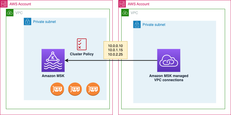
Solution overview
Establishing multi-VPC private connectivity involves turning on this feature for the cluster and configuring the Kafka clients to connect privately to the cluster.
The following are the high-level steps to configure the cluster:
- Enable the multi-VPC private connectivity feature for a subset of authentication schemes that are enabled for your MSK cluster.
- If a Kafka client is in an AWS account that is different than the cluster, attach a resource-based policy to the MSK cluster to authorize IAM principals for creating cross-account connectivity.
- Share the cluster ARN with the IAM principal associated with the Kafka client that needs to create the cross-account access to MSK cluster.
The following are the high-level steps to configure the clients:
- Create a managed VPC endpoint for the client VPC that needs to connect privately to the MSK cluster.
- Update the VPC endpoint’s security group settings to enable outbound connectivity to the MSK cluster.
- Set up the client to use the cluster’s connection string to connect privately to the cluster.
Cluster setup
In this post, we only show the steps for enabling Amazon MSK multi-VPC connectivity for a provisioned cluster.
- To enable Amazon MSK multi-VPC connectivity on your existing cluster, choose Turn on multi-VPC connectivity on the Amazon MSK console.

Note that multi-VPC connectivity cannot be turned on with a cluster that allows unauthenticated access. This is to prevent unauthenticated access from different VPCs. - Select the authentication methods that you allow clients in other VPCs to use.
The list of authentication methods is populated based on your cluster’s security configuration. - Review the settings and choose Turn on selection. After the multi-VPC connectivity is enabled on your cluster, Amazon MSK will create the NLB and VPC endpoint service infrastructure required for private connectivity. Amazon MSK will vend a new set of bootstrap broker strings that can be used for private connectivity. These can be accessed using the View client info option on the Amazon MSK console. The next step is to provide the IAM principals associated with your clients the permissions to connect privately to your cluster. To do this, you need to attach a cluster policy to the cluster.

- Choose Edit cluster policy in the Security section of the cluster details page on the Amazon MSK console.
The new cluster policy allows for defining a Basic or Advanced cluster policy. With the Basic option, you can simply enter AWS account IDs of your client’s VPCs. This policy allows all allowed principals in those AWS accounts to performCreateVPCConnection,GetBootstrapBrokers,DescribeCluster, andDescribeClusterV2actions that are required for creating the cross-VPC connectivity to your cluster. However, in other cases, you may need a more complex policy that allows for additional actions, or principals other than AWS accounts, such as IAM roles, role sessions, IAM users, and more. You can author a cluster policy according to IAM JSON policy guidance and provide that to the cluster in Advanced mode. - Define your cluster policy and choose Save changes.

Client setup
On the client side, first you need to attach an identity policy to the IAM principal who wants to create a managed VPC connection. The identity policy must provide permission for creating a managed VPC connection. The necessary permissions are part of the AWS managed policy AmazonMSKFullAccess.
- In the other AWS account with the IAM principal you configured, use the new Managed VPC connection page on the Amazon MSK console to create Amazon MSK managed VPC connections.
A managed VPC connection maps to an AWS PrivateLink endpoint under the hood, and Amazon MSK uses the managed VPC connection to orchestrate private connectivity to the cluster. You simply need to create the managed VPC connection and pay standard AWS PrivateLink charges for the underlying endpoint.
- Enter the AWS Resource Name (ARN) of the cluster that you want to connect to.
- Choose Verify to verify the cluster information and its minimum requirements for cross-connectivity.
- Select an authentication method from the provided values.
- Choose the VPC ID where your Kafka clients are located, and choose their subnet IDs. You can add more subnets using the Add subnet option.
The specified client subnet must have Availability Zone IDs that match the cluster’s Availability Zone IDs. This makes sure the clients are located in a same physical Availability Zone as the cluster brokers. Amazon MSK uses the port range14001:14100for all authentication methods. You need to select a security group that allows outbound traffic to this port. The following screenshot shows an example. - Review the settings and choose Create connection.

The process will take a few minutes. - When it’s complete, you can obtain the clients’ connection string from the details page of your connection.
- The next step is to update the outbound rules for the VPC endpoint security group to allow communication to the port range
14001:14100.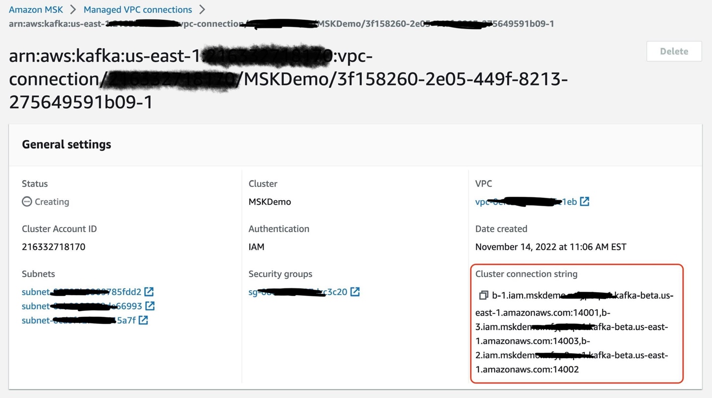
Use the Amazon MSK-managed VPC connection
After you create the managed VPC connection, connecting privately to the cluster is easy. Simply use the new connection string to connect to the cluster. For example, you may connect from an Amazon Elastic Compute Cloud (Amazon EC2) instance on your client VPC. Then run the following command to verify if you can connect and perform actions against the topics in the MSK cluster:

IAM authentication
Before the launch of Amazon MSK multi-VPC connectivity, Kafka clients in other AWS accounts who opted in IAM authentication, needed to assume another IAM role in the cluster’s account. To facilitate this, admins had to create multiple IAM roles and write a trust policy that allows authenticated principals from the client’s accounts to assume corresponding roles through the sts:AssumeRole API call. This approach was challenging to scale when the number of VPCs or AWS accounts grew. With the launch of this cluster policy, cross-account access control is now simplified because you can attach a cluster policy to your clusters to specify which cross-account clients have what permissions on resources within the cluster.
This capability allows you to manage all access to the cluster and topics in one place. For example, you can control which IAM principals have write access to certain topics, and which principals can only read from them. Users who are using IAM client authentication can also add permissions for required kafka-cluster actions in the cluster resource policy.
Availability and pricing
You can now use Amazon MSK multi-VPC connectivity in all commercial Regions where Amazon MSK is offered, including China and GovCloud (US) Regions.
You pay $0.006 per GB data processed for private connectivity and $0.0225 per private connectivity hour per authentication scheme in US East (Ohio). Refer to our Pricing page for more details.
Conclusion
With Amazon MSK multi-VPC private connectivity, you can now privately access your MSK brokers from your client applications in another VPC within the same AWS account or another AWS account, with minimal configuration. You no longer have to create, manage, and update multiple networking resources in multiple VPCs, or make Amazon MSK configuration changes to connect your Kafka clients across VPCs and accounts. Amazon MSK creates and manages the resources for you. With Cluster policy support, you can easily provide your cross-account client principals permissions to connect privately to your MSK cluster. Further, if you are using IAM client authentication, you can also leverage the cluster policy to centrally control clients’ permissions to perform operations on the cluster. Use the Amazon MSK multi-VPC connectivity and the cluster policy feature today to simplify your secure connectivity infrastructure.
For further reading on Amazon MSK, visit the official product page and our AWS Documentation.
About the authors
 Ali Alemi is a Streaming Specialist Solutions Architect at AWS. Ali advises AWS customers with architectural best practices and helps them design real-time analytics data systems that are reliable, secure, efficient, and cost-effective. He works backward from customers’ use cases and designs data solutions to solve their business problems. Prior to joining AWS, Ali supported several public sector customers and AWS consulting partners in their application modernization journey and migration to the cloud.
 Rajeev Chakrabarti is a Kinesis specialist solutions architect.
Amazon Redshift is a fast, scalable, secure, and fully managed cloud data warehouse that makes it simple and cost-effective to analyze all your data using standard SQL and your existing ETL (extract, transform, and load), business intelligence (BI), and reporting tools. Tens of thousands of customers use Amazon Redshift to process exabytes of data per day and power analytics workloads such as BI, predictive analytics, and real-time streaming analytics. Amazon Redshift Serverless makes it convenient for you to run and scale analytics without having to provision and manage data warehouses. With Redshift Serverless, data analysts, developers, and data scientists can now use Amazon Redshift to get insights from data in seconds by loading data into and querying records from the data warehouse.
As a data engineer or application developer, for some use cases, you want to interact with the Redshift Serverless data warehouse to load or query data with a simple API endpoint without having to manage persistent connections. With the Amazon Redshift Data API, you can interact with Redshift Serverless without having to configure JDBC or ODBC. This makes it easier and more secure to work with Redshift Serverless and opens up new use cases.
This post explains how to use the Data API with Redshift Serverless from the AWS Command Line Interface (AWS CLI) and Python. If you want to use the Data API with Amazon Redshift clusters, refer to Using the Amazon Redshift Data API to interact with Amazon Redshift clusters.
Introducing the Data API
The Data API enables you to seamlessly access data from Redshift Serverless with all types of traditional, cloud-native, and containerized serverless web service-based applications and event-driven applications.
The following diagram illustrates this architecture.

The Data API simplifies data access, ingest, and egress from programming languages and platforms supported by the AWS SDK such as Python, Go, Java, Node.js, PHP, Ruby, and C++.
The Data API simplifies access to Amazon Redshift by eliminating the need for configuring drivers and managing database connections. Instead, you can run SQL commands to Redshift Serverless by simply calling a secured API endpoint provided by the Data API. The Data API takes care of managing database connections and buffering data. The Data API is asynchronous, so you can retrieve your results later. Your query results are stored for 24 hours. The Data API federates AWS Identity and Access Management (IAM) credentials so you can use identity providers like Okta or Azure Active Directory or database credentials stored in Secrets Manager without passing database credentials in API calls.
For customers using AWS Lambda, the Data API provides a secure way to access your database without the additional overhead for Lambda functions to be launched in an Amazon VPC. Integration with the AWS SDK provides a programmatic interface to run SQL statements and retrieve results asynchronously.
Relevant use cases
The Data API is not a replacement for JDBC and ODBC drivers, and is suitable for use cases where you don’t need a persistent connection to a serverless data warehouse. It’s applicable in the following use cases:
- Accessing Amazon Redshift from custom applications with any programming language supported by the AWS SDK. This enables you to integrate web service-based applications to access data from Amazon Redshift using an API to run SQL statements. For example, you can run SQL from JavaScript.
- Building a serverless data processing workflow.
- Designing asynchronous web dashboards because the Data API lets you run long-running queries without having to wait for them to complete.
- Running your query one time and retrieving the results multiple times without having to run the query again within 24 hours.
- Building your ETL pipelines with AWS Step Functions, Lambda, and stored procedures.
- Having simplified access to Amazon Redshift from Amazon SageMaker and Jupyter notebooks.
- Building event-driven applications with Amazon EventBridge and Lambda.
- Scheduling SQL scripts to simplify data load, unload, and refresh of materialized views.
The Data API GitHub repository provides examples for different use cases for both Redshift Serverless and provisioned clusters.
Create a Redshift Serverless workgroup
If you haven’t already created a Redshift Serverless data warehouse, or want to create a new one, refer to the Getting Started Guide. This guide walks you through the steps of creating a namespace and workgroup with their names as default. Also, ensure that you have created an IAM role and make sure that the IAM role you attach to your Redshift Serverless namespace has AmazonS3ReadOnlyAccess permission. You can use the AWS Management Console to create an IAM role and assign Amazon Simple Storage Service (Amazon S3) privileges (refer to Loading in data from Amazon S3). In this post, we create a table and load data using the COPY command.
Prerequisites for using the Data API
You must be authorized to access the Data API. Amazon Redshift provides the RedshiftDataFullAccess managed policy, which offers full access to Data API. This policy also allows access to Redshift Serverless workgroups, Secrets Manager, and API operations needed to authenticate and access a Redshift Serverless workgroup by using IAM credentials.
You can also create your own IAM policy that allows access to specific resources by starting with RedshiftDataFullAccess as a template.
The Data API allows you to access your database either using your IAM credentials or secrets stored in Secrets Manager. In this post, we use IAM credentials.
When you federate your IAM credentials to connect with Amazon Redshift, it automatically creates a database user for the IAM user that is being used. It uses the GetCredentials API to get temporary database credentials. If you want to provide specific database privileges to your users with this API, you can use an IAM role with the tag name RedshiftDBRoles with a list of roles separated by colons. For example, if you want to assign database roles such as sales and analyst, you can have a value sales:analyst assigned to RedshiftDBRoles.
Use the Data API from the AWS CLI
You can use the Data API from the AWS CLI to interact with the Redshift Serverless workgroup and namespace. For instructions on configuring the AWS CLI, see Setting up the AWS CLI. The Amazon Redshift Serverless CLI (aws redshift-serverless) is a part of AWS CLI that lets you manage Amazon Redshift workgroups and namespaces, such as creating, deleting, setting usage limits, tagging resource, and more. The Data API provides a command line interface to the AWS CLI (aws redshift-data) that allows you to interact with the databases in Redshift Serverless.
You can invoke help using the following command:
The following table shows you the different commands available with the Data API CLI.
| Command | Description |
list-databases | Lists the databases in a workgroup. |
list-schemas | Lists the schemas in a database. You can filter this by a matching schema pattern. |
list-tables | Lists the tables in a database. You can filter the tables list by a schema name pattern, a matching table name pattern, or a combination of both. |
describe-table | Describes the detailed information about a table including column metadata. |
execute-statement | Runs a SQL statement, which can be SELECT, DML, DDL, COPY, or UNLOAD. |
batch-execute-statement | Runs multiple SQL statements in a batch as a part of single transaction. The statements can be SELECT, DML, DDL, COPY, or UNLOAD. |
cancel-statement | Cancels a running query. To be canceled, a query must not be in the FINISHED or FAILED state. |
describe-statement | Describes the details of a specific SQL statement run. The information includes when the query started, when it finished, the number of rows processed, and the SQL statement. |
list-statements | Lists the SQL statements in the last 24 hours. By default, only finished statements are shown. |
get-statement-result | Fetches the temporarily cached result of the query. The result set contains the complete result set and the column metadata. You can paginate through a set of records to retrieve the entire result as needed. |
If you want to get help on a specific command, run the following command:
Now we look at how you can use these commands.
List databases
Most organizations use a single database in their Amazon Redshift workgroup. You can use the following command to list the databases in your Serverless endpoint. This operation requires you to connect to a database and therefore requires database credentials.
List schemas
Similar to listing databases, you can list your schemas by using the list-schemas command:
If you have several schemas that match demo (demo, demo2, demo3, and so on), you can optionally provide a pattern to filter your results matching to that pattern:
List tables
The Data API provides a simple command, list-tables, to list tables in your database. You might have thousands of tables in a schema; the Data API lets you paginate your result set or filter the table list by providing filter conditions.
You can search across your schema with table-pattern; for example, you can filter the table list by a table name prefix across all your schemas in the database or filter your tables list in a specific schema pattern by using schema-pattern.
The following is a code example that uses both:
Run SQL commands
You can run SELECT, DML, DDL, COPY, or UNLOAD commands for Amazon Redshift with the Data API. You can optionally specify the –with-event option if you want to send an event to EventBridge after the query run, then the Data API will send the event with queryId and final run status.
Create a schema
Let’s use the Data API to see how you can create a schema. The following command lets you create a schema in your database. You don’t have to run this SQL if you have pre-created the schema. You have to specify –-sql to specify your SQL commands.
The following shows an example output of execute-statement:
We discuss later in this post how you can check the status of a SQL that you ran with execute-statement.
Create a table
You can use the following command to create a table with the CLI:
Load sample data
The COPY command lets you load bulk data into your table in Amazon Redshift. You can use the following command to load data into the table we created earlier:
Retrieve data
The following query uses the table we created earlier:
The following shows an example output:
You can fetch results using the statement ID that you receive as an output of execute-statement.
Check the status of a statement
You can check the status of your statement by using describe-statement. The output for describe-statement provides additional details such as PID, query duration, number of rows in and size of the result set, and the query ID given by Amazon Redshift. You have to specify the statement ID that you get when you run the execute-statement command. See the following command:
The following is an example output:
The status of a statement can be STARTED, FINISHED, ABORTED, or FAILED.
Run SQL statements with parameters
You can run SQL statements with parameters. The following example uses two named parameters in the SQL that is specified using a name-value pair:
The describe-statement returns QueryParameters along with QueryString.
You can map the name-value pair in the parameters list to one or more parameters in the SQL text, and the name-value parameter can be in random order. You can’t specify a NULL value or zero-length value as a parameter.
Cancel a running statement
If your query is still running, you can use cancel-statement to cancel a SQL query. See the following command:
Fetch results from your query
You can fetch the query results by using get-statement-result. The query result is stored for 24 hours. See the following command:
The output of the result contains metadata such as the number of records fetched, column metadata, and a token for pagination.
Run multiple SQL statements
You can run multiple SELECT, DML, DDL, COPY, or UNLOAD commands for Amazon Redshift in a single transaction with the Data API. The batch-execute-statement enables you to create tables and run multiple COPY commands or create temporary tables as part of your reporting system and run queries on that temporary table. See the following code:
The describe-statement for a multi-statement query shows the status of all sub-statements:
{
In the preceding example, we had two SQL statements and therefore the output includes the ID for the SQL statements as 23d99d7f-fd13-4686-92c8-e2c279715c21:1 and 23d99d7f-fd13-4686-92c8-e2c279715c21:2. Each sub-statement of a batch SQL statement has a status, and the status of the batch statement is updated with the status of the last sub-statement. For example, if the last statement has status FAILED, then the status of the batch statement shows as FAILED.
You can fetch query results for each statement separately. In our example, the first statement is a SQL statement to create a temporary table, so there are no results to retrieve for the first statement. You can retrieve the result set for the second statement by providing the statement ID for the sub-statement:
Use the Data API with Secrets Manager
The Data API allows you to use database credentials stored in Secrets Manager. You can create a secret type as Other type of secret and then specify username and password. Note you can’t choose an Amazon Redshift cluster because Redshift Serverless is different than a cluster.

Let’s assume that you created a secret key for your credentials as defaultWG. You can use the secret-arn parameter to pass your secret key as follows:
Export the data
Amazon Redshift allows you to export from database tables to a set of files in an S3 bucket by using the UNLOAD command with a SELECT statement. You can unload data in either text or Parquet format. The following command shows you an example of how to use the data lake export with the Data API:
You can use batch-execute-statement if you want to use multiple statements with UNLOAD or combine UNLOAD with other SQL statements.
Use the Data API from the AWS SDK
You can use the Data API in any of the programming languages supported by the AWS SDK. For this post, we use the AWS SDK for Python (Boto3) as an example to illustrate the capabilities of the Data API.
We first import the Boto3 package and establish a session:
Get a client object
You can create a client object from the boto3.Session object and using RedshiftData:
If you don’t want to create a session, your client is as simple as the following code:
Run a statement
The following example code uses the Secrets Manager key to run a statement. For this post, we use the table we created earlier. You can use DDL, DML, COPY, and UNLOAD in the SQL parameter:
As we discussed earlier, running a query is asynchronous; running a statement returns an ExecuteStatementOutput, which includes the statement ID.
If you want to publish an event to EventBridge when the statement is complete, you can use the additional parameter WithEvent set to true:
Describe a statement
You can use describe\_statement to find the status of the query and number of records retrieved:
Fetch results from your query
You can use get\_statement\_result to retrieve results for your query if your query is complete:
The get\_statement\_result command returns a JSON object that includes metadata for the result and the actual result set. You might need to process the data to format the result if you want to display it in a user-friendly format.
Fetch and format results
For this post, we demonstrate how to format the results with the Pandas framework. The post\_process function processes the metadata and results to populate a DataFrame. The query function retrieves the result from a database in an Amazon Redshift cluster. See the following code:
In this post, we demonstrated using the Data API with Python with Redshift Serverless. However, you can use the Data API with other programming languages supported by the AWS SDK. You can read how Roche democratized access to Amazon Redshift data using the Data API with Google Sheets. You can also address this type of use case with Redshift Serverless.
Best practices
We recommend the following best practices when using the Data API:
- Federate your IAM credentials to the database to connect with Amazon Redshift. Redshift Serverless allows users to get temporary database credentials with
GetCredentials. Redshift Serverless scopes the access to the specific IAM user and the database user is automatically created. - Use a custom policy to provide fine-grained access to the Data API in the production environment if you don’t want your users to use temporary credentials. You have to use Secrets Manager to manage your credentials in such use cases.
- Don’t retrieve a large amount of data from your client and use the UNLOAD command to export the query results to Amazon S3. You’re limited to retrieving only 100 MB of data with the Data API.
- Don’t forget to retrieve your results within 24 hours; results are stored only for 24 hours.
Conclusion
In this post, we introduced how to use the Data API with Redshift Serverless. We also demonstrated how to use the Data API from the Amazon Redshift CLI and Python using the AWS SDK. Additionally, we discussed best practices for using the Data API.
To learn more, refer to Using the Amazon Redshift Data API or visit the Data API GitHub repository for code examples.
About the authors
 Debu Panda is a Senior Manager, Product Management at AWS, is an industry leader in analytics, application platform, and database technologies, and has more than 25 years of experience in the IT world. Debu has published numerous articles on analytics, enterprise Java, and databases and has presented at multiple conferences such as re:Invent, Oracle Open World, and Java One. He is lead author of the EJB 3 in Action (Manning Publications 2007, 2014) and Middleware Management (Packt).
 Fei Peng is a Software Dev Engineer working in the Amazon Redshift team.
This is a guest post co-written with Jonatan Selsing and Moses Arthur from Novo Nordisk.
This is the second post of a three-part series detailing how Novo Nordisk, a large pharmaceutical enterprise, partnered with AWS Professional Services to build a scalable and secure data and analytics platform. The first post of this series describes the overall architecture and how Novo Nordisk built a decentralized data mesh architecture, including Amazon Athena as the data query engine. The third post will show how end-users can consume data from their tool of choice, without compromising data governance. This will include how to configure Okta, AWS Lake Formation, and a business intelligence tool to enable SAML-based federated use of Athena for an enterprise BI activity.
When building a scalable data architecture on AWS, giving autonomy and ownership to the data domains are crucial for the success of the platform. By providing the right mix of freedom and control to those people with the business domain knowledge, your business can maximize value from the data as quickly and effectively as possible. The challenge facing organizations, however, is how to provide the right balance between freedom and control. At the same time, data is a strategic asset that needs to be protected with the highest degree of rigor. How can organizations strike the right balance between freedom and control?
In this post, you will learn how to build decentralized governance with Lake Formation and AWS Identity and Access Management (IAM) using attribute-based access control (ABAC). We discuss some of the patterns we use, including Amazon Cognito identity pool federation using ABAC in permission policies, and Okta-based SAML federation with ABAC enforcement on role trust policies.
Solution overview
In the first post of this series, we explained how Novo Nordisk and AWS Professional Services built a modern data architecture based on data mesh tenets. This architecture enables data governance on distributed data domains, using an end-to-end solution to create data products and providing federated data access control. This post dives into three elements of the solution:
- How IAM roles and Lake Formation are used to manage data access across data domains
- How data access control is enforced at scale, using a group membership mapping with an ABAC pattern
- How the system maintains state across the different layers, so that the ecosystem of trust is configured appropriately
From the end-user perspective, the objective of the mechanisms described in this post is to enable simplified data access from the different analytics services adopted by Novo Nordisk, such as those provided by software as a service (SaaS) vendors like Databricks, or self-hosted ones such as JupyterHub. At the same time, the platform must guarantee that any change in a dataset is immediately reflected at the service user interface. The following figure illustrates at a high level the expected behavior.
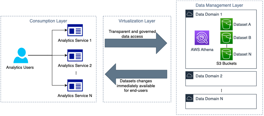
Following the layer nomenclature established in the first post, the services are created and managed in the consumption layer. The domain accounts are created and managed in the data management layer. Because changes can occur from both layers, continuous communication in both directions is required. The state information is kept in the virtualization layer along with the communication protocols. Additionally, at sign-in time, the services need information about data resources required to provide data access abstraction.
Managing data access
The data access control in this architecture is designed around the core principle that all access is encapsulated in isolated IAM role sessions. The layer pattern that we described in the first post ensures that the creation and curation of the IAM role policies involved can be delegated to the different data management ecosystems. Each data management platform integrated can use their own data access mechanisms, with the unique requirement that the data is accessed via specific IAM roles.
To illustrate the potential mechanisms that can be used by data management solutions, we show two examples of data access permission mechanisms used by two different data management solutions. Both systems utilize the same trust policies as described in the following sections, but have a completely different permission space.
Example 1: Identity-based ABAC policies
The first mechanism we discuss is an ABAC role that provides access to a home-like data storage area, where users can share within their departments and with the wider organization in a structure that mimics the organizational structure. Here, we don’t utilize the group names, but instead forward user attributes from the corporate Active Directory directly into the permission policy through claim overrides. We do this by having the corporate Active Directory as the identity provider (IdP) for the Amazon Cognito user pool and mapping the relevant IdP attributes to user pool attributes. Then, in the Amazon Cognito identity pool, we map the user pool attributes to session tags to use them for access control. Custom overrides can be included in the claim mapping, through the use of a pre token generation Lambda trigger. This way, claims from AD can be mapped to Amazon Cognito user pool attributes and then ultimately used in the Amazon Cognito identity pool to control IAM role permissions. The following is an example of an IAM policy with sessions tags:
This role is then embedded in the analytics layer (together with the data domain roles) and assumed on behalf of the user. This enables users to mix and match between data domains—as well as utilizing private and public data paths that aren’t necessarily tied to any data domain. For more examples of how ABAC can be used with permission policies, refer to How to scale your authorization needs by using attribute-based access control with S3.
Example 2: Lake Formation name-based access controls
In the data management solution named Novo Nordisk Enterprise Datahub (NNEDH), which we introduced in the first post, we use Lake Formation to enable standardized data access. The NNEDH datasets are registered in the Lake Formation Data Catalog as databases and tables, and permissions are granted using the named resource method. The following screenshot shows an example of these permissions.
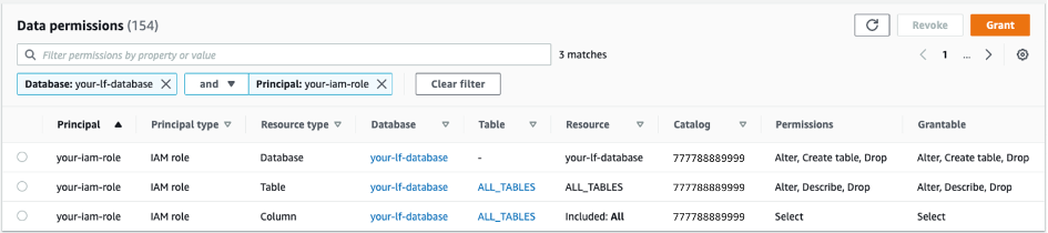
In this approach, data access governance is delegated to Lake Formation. Every data domain in NNEDH has isolated permissions synthesized by NNEDH as the central governance management layer. This is a similar pattern to what is adopted for other domain-oriented data management solutions. Refer to Use an event-driven architecture to build a data mesh on AWS for an example of tag-based access control in Lake Formation.
These patterns don’t exclude implementations of peer-to-peer type data sharing mechanisms, such as those that can be achieved using AWS Resource Access Manager (AWS RAM), where a single IAM role session can have permissions that span across accounts.
Delegating role access to the consumption later
The following figure illustrates the data access workflow from an external service.

The workflow steps are as follows:
- A user authenticates on an IdP used by the analytics tool that they are trying to access. A wide range of analytics tools are supported by Novo Nordisk platform, such as Databricks and JupyterHub, and the IdP can be either SAML or OIDC type depending on the capabilities of the third-party tool. In this example, an Okta SAML application is used to sign into a third-party analytics tool, and an IAM SAML IdP is configured in the data domain AWS account to federate with the external IdP. The third post of this series describes how to set up an Okta SAML application for IAM role federation on Athena.
- The SAML assertion obtained during the sign-in process is used to request temporary security credentials of an IAM role through the AssumeRole operation. In this example, the SAML assertion is used on
AssumeRoleWithSAMLoperation. For OpenID Connect-compatible IdPs, the operationAssumeRoleWithWebIdentitymust be used with the JWT. The SAML attributes in the assertion or the claims in the token can be generated at sign-in time, to ensure that the group memberships are forwarded, for the ABAC policy pattern described in the following sections. - The analytics tool, such as Databricks or JupyterHub, abstracts the usage of the IAM role session credentials in the tool itself, and data can be accessed directly according to the permissions of the IAM role assumed. This pattern is similar in nature to IAM passthrough as implemented by Databricks, but in Novo Nordisk it’s extended across all analytics services. In this example, the analytics tool accesses the data lake on Amazon Simple Storage Service (Amazon S3) through Athena queries.
As the data mesh pattern expands across domains covering more downstream services, we need a mechanism to keep IdPs and IAM role trusts continuously updated. We come back to this part later in the post, but first we explain how role access is managed at scale.
Attribute-based trust policies
In previous sections, we emphasized that this architecture relies on IAM roles for data access control. Each data management platform can implement its own data access control method using IAM roles, such as identity-based policies or Lake Formation access control. For data consumption, it’s crucial that these IAM roles are only assumable by users that are part of Active Directory groups with the appropriate entitlements to use the role. To implement this at scale, the IAM role’s trust policy uses ABAC.
When a user authenticates on the external IdP of the consumption layer, we add in the access token a claim derived from their Active Directory groups. This claim is propagated by theAssumeRoleoperation into the trust policy of the IAM role, where it is compared with the expected Active Directory group. Only users that belong to the expected groups can assume the role. This mechanism is illustrated in the following figure.
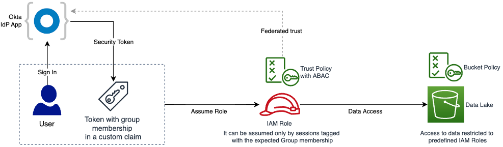
Translating group membership to attributes
To enforce the group membership entitlement at the role assumption level, we need a way to compare the required group membership with the group memberships that a user comes with in their IAM role session. To achieve this, we use a form of ABAC, where we have a way to represent the sum of context-relevant group memberships in a single attribute. A single IAM role session tag value is limited to 256 characters. The corresponding limit for SAML assertions is 100,000 characters, so for systems where a very large number of either roles or group-type mappings are required, SAML can support a wider range of configurations.
In our case, we have opted for a compression algorithm that takes a group name and compresses it to a 4-character string hash. This means that, together with a group-separation character, we can fit 51 groups in a single attribute. This gets pushed down to approximately 20 groups for OIDC type role assumption due to the PackedPolicySize, but is higher for a SAML-based flow. This has shown to be sufficient for our case. There is a risk that two different groups could hash to the same character combination; however, we have checked that there are no collisions in the existing groups. To mitigate this risk going forward, we have introduced guardrails in multiples places. First, before adding new groups entitlements in the virtualization layer, we check if there’s a hash collision with any existing group. When a duplicated group is attempted to be added, our service team is notified and we can react accordingly. But as stated earlier, there is a low probability of clashes, so the flexibility this provides outweighs the overhead associated with managing clashes (we have not had any yet). We additionally enforce this at SAML assertion creation time as well, to ensure that there are no duplicated groups in the users group list, and in cases of duplication, we remove both entirely. This means malicious actors can at most limit the access of other users, but not gain unauthorized access.
Enforcing audit functionality across sessions
As mentioned in the first post, on top of governance, there are strict requirements around auditability of data accesses. This means that for all data access requests, it must be possible to trace the specific user across services and retain this information. We achieve this by setting (and enforcing) a source identity for all role sessions and make sure to propagate enterprise identity to this attribute. We use a combination of Okta inline hooks and SAML session tags to achieve this. This means that the AWS CloudTrail logs for an IAM role session have the following information:
On the IAM role level, we can enforce the required attribute configuration with the following example trust policy. This is an example for a SAML-based app. We support the same patterns through OpenID Connect IdPs.
We now go through the elements of an IAM role trust policy, based on the following example:
The policy contains the following details:
- The
Principalstatement should point to the list of apps that are served through the consumption layer. These can be Azure app registrations, Okta apps, or Amazon Cognito app clients. This means that SAML assertions (in the case of SAML-based flows) minted from these applications can be used to run the operationAssumeRoleWithSamlif the remaining elements are also satisfied. - The
Actionstatement includes the required permissions for theAssumeRolecall to succeed, including adding the contextual information to the role session. - In the first condition, the audience of the assertion needs to be targeting AWS.
- In the second condition, there are two
StringLikerequirements:- A requirement on the source identity as the naming convention to follow at Novo Nordisk (users must come with enterprise identity, following our audit requirements).
- The
aws:RequestTag/GroupHashneeds to bexxxx, which represents the hashed group name mentioned in the upper section.
- Lastly, we enforce that sessions can’t be started without setting the source identity.
This policy enforces that all calls are from recognized services, include auditability, have the right target, and enforces that the user has the right group memberships.
Building a central overview of governance and trust
In this section, we discuss how Novo Nordisk keeps track of the relevant group-role relations and maps these at sign-in time.
Entitlements
In Novo Nordisk, all accesses are based on Active Directory group memberships. There is no user-based access. Because this pattern is so central, we have extended this access philosophy into our data accesses. As mentioned earlier, at sign-in time, the hooks need to be able to know which roles to assume for a given user, given this user’s group membership. We have modeled this data in Amazon DynamoDB, where just-in-time provisioning ensures that only the required user group memberships are available. By building our application around the use of groups, and by having the group propagation done by the application code, we avoid having to make a more general Active Directory integration, which would, for a company the size of Novo Nordisk, severely impact the application, simply due to the volume of users and groups.
The DynamoDB entitlement table contains all relevant information for all roles and services, including role ARNs and IdP ARNs. This means that when users log in to their analytics services, the sign-in hook can construct the required information for the Roles SAML attribute.
When new data domains are added to the data management layer, the data management layer needs to communicate both the role information and the group name that gives access to the role.
Single sign-on hub for analytics services
When scaling this permission model and data management pattern to a large enterprise such as Novo Nordisk, we ended up creating a large number of IAM roles distributed across different accounts. Then, a solution is required to map and provide access for end-users to the required IAM role. To simplify user access to multiple data sources and analytics tools, Novo Nordisk developed a single sign-on hub for analytics services. From the end-user perspective, this is a web interface that glues together different offerings in a unified system, making it a one-stop tool for data and analytics needs. When signing in to each of the analytical offerings, the authenticated sessions are forwarded, so users never have to reauthenticate.
Common for all the services supported in the consumption layer is that we can run a piece of application code at sign-in time, allowing sign-in time permissions to be calculated. The hooks that achieve this functionality can, for instance, be run by Okta inline hooks. This means that each of the target analytics services can have custom code to translate relevant contextual information or provide other types of automations for the role forwarding.
The sign-in flow is demonstrated in the following figure.
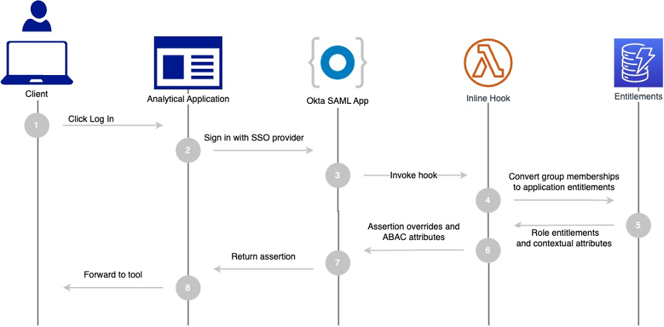
The workflow steps are as follows:
- A user accesses an analytical service such as Databricks in the Novo Nordisk analytics hub.
- The service uses Okta as the SAML-based IdP.
- Okta invokes an AWS Lambda-based SAML assertion inline hook.
- The hook uses the entitlement database, converting application-relevant group memberships into role entitlements.
- Relevant contextual information is returned from the entitlement database.
- The Lambda-based hook adds new SAML attributes to the SAML assertion, including the hashed group memberships and other contextual information such as source identity.
- A modified SAML assertion is used to sign users in to the analytical service.
- The user can now use the analytical tool with active IAM role sessions.
Synchronizing role trust
The preceding section gives an overview of how federation works in this solution. Now we can go through how we ensure that all participating AWS environments and accounts are in sync with the latest configuration.
From the end-user perspective, the synchronization mechanism must ensure that every analytics service instantiated can access the data domains assigned to the groups that the user belongs to. Also, changes in data domains—such as granting data access to an Active Directory group—must be effective immediately to every analytics service.
Two event-based mechanisms are used to maintain all the layers synchronized, as detailed in this section.
Synchronize data access control on the data management layer with changes to services in the consumption layer
As describe in the previous section, the IAM roles used for data access are created and managed by the data management layer. These IAM roles have a trust policy providing federated access to the external IdPs used by the analytics tools of the consumption layer. It implies that for every new analytical service created with a different IDP, the IAM roles used for data access on data domains must be updated to trust this new IdP.
Using NNEDH as an example of a data management solution, the synchronization mechanism is demonstrated in the following figure.
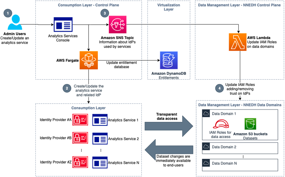
Taking as an example a scenario where a new analytics service is created, the steps in this workflow are as follows:
- A user with access to the administration console of the consumption layer instantiates a new analytics service, such as JupyterHub.
- A job running on AWS Fargate creates the resources needed for this new analytics service, such as an Amazon Elastic Compute Cloud (Amazon EC2) instance for JupyterHub, and the IdP required, such as a new SAML IdP.
- When the IdP is created in the previous step, an event is added in an Amazon Simple Notification Service (Amazon SNS) topic with its details, such as name and SAML metadata.
- In the NNEDH control plane, a Lambda job is triggered by new events on this SNS topic. This job creates the IAM IdP, if needed, and updates the trust policy of the required IAM roles in all the AWS accounts used as data domains, adding the trust on the IdP used by the new analytics service.
In this architecture, all the update steps are event-triggered and scalable. This means that users of new analytics services can access their datasets almost instantaneously when they are created. In the same way, when a service is removed, the federation to the IdP is automatically removed if not used by other services.
Propagate changes on data domains to analytics services
Changes to data domains, such as the creation of a new S3 bucket used as a dataset, or adding or removing data access to a group, must be reflected immediately on analytics services of the consumption layer. To accomplish it, a mechanism is used to synchronize the entitlement database with the relevant changes made in NNEDH. This flow is demonstrated in the following figure.
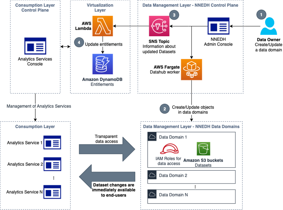
Taking as an example a scenario where access to a specific dataset is granted to a new group, the steps in this workflow are as follows:
- Using the NNEDH admin console, a data owner approves a dataset sharing request that grants access on a dataset to an Active Directory group.
- In the AWS account of the related data domain, the dataset components such as the S3 bucket and Lake Formation are updated to provide data access to the new group. The cross-account data sharing in Lake Formation uses AWS RAM.
- An event is added in an SNS topic with the current details about this dataset, such as the location of the S3 bucket and the groups that currently have access to it.
- In the virtualization layer, the updated information from the data management layer is used to update the entitlement database in DynamoDB.
These steps make sure that changes on data domains are automatically and immediately reflected on the entitlement database, which is used to provide data access to all the analytics services of the consumption layer.
Limitations
Many of these patterns rely on the analytical tool to support a clever use of IAM roles. When this is not the case, the platform teams themselves need to develop custom functionality at the host level to ensure that role accesses are correctly controlled. This, for example, includes writing custom authenticators for JupyterHub.
Conclusion
This post shows an approach to building a scalable and secure data and analytics platform. It showcases some of the mechanisms used at Novo Nordisk and how to strike the right balance between freedom and control. The architecture laid out in the first post in this series enables layer independence, and exposes some extremely useful primitives for data access and governance. We make heavy use of contextual attributes to modulate role permissions at the session level, which provide just-in-time permissions. These permissions are propagated at a scale, across data domains. The upside is that a lot of the complexity related to managing data access permission can be delegated to the relevant business groups, while enabling the end-user consumers of data to think as little as possible about data accesses and focus on providing value for the business use cases. In the case of Novo Nordisk, they can provide better outcomes for patients and acceleration innovation.
The next post in this series describes how end-users can consume data from their analytics tool of choice, aligned with the data access controls detailed in this post.
About the Authors
 Jonatan Selsing is former research scientist with a PhD in astrophysics that has turned to the cloud. He is currently the Lead Cloud Engineer at Novo Nordisk, where he enables data and analytics workloads at scale. With an emphasis on reducing the total cost of ownership of cloud-based workloads, while giving full benefit of the advantages of cloud, he designs, builds, and maintains solutions that enable research for future medicines.
 Hassen Riahi is a Sr. Data Architect at AWS Professional Services. He holds a PhD in Mathematics & Computer Science on large-scale data management. He works with AWS customers on building data-driven solutions.
 Alessandro Fior is a Sr. Data Architect at AWS Professional Services. He is passionate about designing and building modern and scalable data platforms that accelerate companies to extract value from their data.
 Moses Arthur comes from a mathematics and computational research background and holds a PhD in Computational Intelligence specialized in Graph Mining. He is currently a Cloud Product Engineer at Novo Nordisk, building GxP-compliant enterprise data lakes and analytics platforms for Novo Nordisk global factories producing digitalized medical products.
 Anwar Rizal is a Senior Machine Learning consultant based in Paris. He works with AWS customers to develop data and AI solutions to sustainably grow their business.
 Kumari Ramar is an Agile certified and PMP certified Senior Engagement Manager at AWS Professional Services. She delivers data and AI/ML solutions that speed up cross-system analytics and machine learning models, which enable enterprises to make data-driven decisions and drive new innovations.
AWS Glue is a serverless data integration service that makes it simple to discover, prepare, and combine data for analytics, machine learning (ML), and application development. You can use AWS Glue to create, run, and monitor data integration and ETL (extract, transform, and load) pipelines and catalog your assets across multiple data stores.
One of the most common questions we get from customers is how to effectively monitor and optimize costs on AWS Glue for Spark. The diversity of features and pricing options for AWS Glue offers the flexibility to effectively manage the cost of your data workloads and still keep the performance and capacity as per your business needs. Although the fundamental process of cost optimization for AWS Glue workloads remains the same, you can monitor job runs and analyze the costs and usage to find savings and take action to implement improvements to the code or configurations.
In this post, we demonstrate a tactical approach to help you manage and reduce cost through monitoring and optimization techniques on top of your AWS Glue workloads.
Monitor overall costs on AWS Glue for Apache Spark
AWS Glue for Apache Spark charges an hourly rate in 1-second increments with a minimum of 1 minute based on the number of data processing units (DPUs). Learn more in AWS Glue Pricing. This section describes a way to monitor overall costs on AWS Glue for Apache Spark.
AWS Cost Explorer
In AWS Cost Explorer, you can see overall trends of DPU hours. Complete the following steps:
- On the Cost Explorer console, create a new cost and usage report.
- For Service, choose Glue.
- For Usage type, choose the following options:
- Choose <Region>-ETL-DPU-Hour (DPU-Hour) for standard jobs.
- Choose <Region>-ETL-Flex-DPU-Hour (DPU-Hour) for Flex jobs.
- Choose <Region>-GlueInteractiveSession-DPU-Hour (DPU-Hour) for interactive sessions.
- Choose Apply.
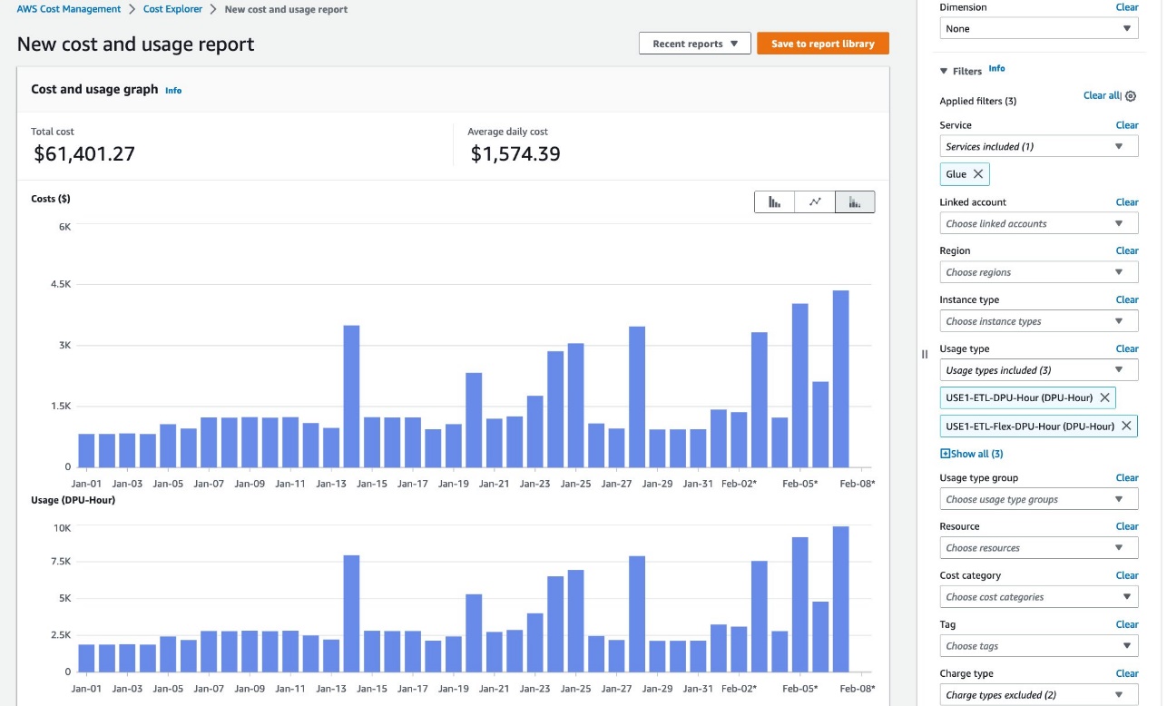
Learn more in Analyzing your costs with AWS Cost Explorer.
Monitor individual job run costs
This section describes a way to monitor individual job run costs on AWS Glue for Apache Spark. There are two options to achieve this.
AWS Glue Studio Monitoring page
On the Monitoring page in AWS Glue Studio, you can monitor the DPU hours you spent on a specific job run. The following screenshot shows three job runs that processed the same dataset; the first job run spent 0.66 DPU hours, and the second spent 0.44 DPU hours. The third one with Flex spent only 0.33 DPU hours.

GetJobRun and GetJobRuns APIs
The DPU hour values per job run can be retrieved through AWS APIs.
For auto scaling jobs and Flex jobs, the field DPUSeconds is available in GetJobRun and GetJobRuns API responses:
The field DPUSeconds returns 1137.0. This means 0.32 DPU hours which can be calculated in 1137.0/(60*60)=0.32.
For the other standard jobs without auto scaling, the field DPUSeconds is not available:
For these jobs, you can calculate DPU hours by ExecutionTime*MaxCapacity/(60*60). Then you get 0.44 DPU hour by 157*10/(60*60)=0.44. Note that AWS Glue versions 2.0 and later have a 1-minute minimum billing.
AWS CloudFormation template
Because DPU hours can be retrieved through the GetJobRun and GetJobRuns APIs, you can integrate this with other services like Amazon CloudWatch to monitor trends of consumed DPU hours over time. For example, you can configure an Amazon EventBridge rule to invoke an AWS Lambda function to publish CloudWatch metrics every time AWS Glue jobs finish.
To help you configure that quickly, we provide an AWS CloudFormation template. You can review and customize it to suit your needs. Some of the resources this stack deploys incur costs when in use.
The CloudFormation template generates the following resources:
- AWS Identity and Access Management (IAM) role
- Lambda function
- EventBridge rule
To create your resources, complete the following steps:
- Sign in to the AWS CloudFormation console.
- Choose Launch Stack:
- Choose Next.
- Choose Next.
- On the next page, choose Next.
- Review the details on the final page and select I acknowledge that AWS CloudFormation might create IAM resources.
- Choose Create stack.
Stack creation can take up to 3 minutes.
After you complete the stack creation, when AWS Glue jobs finish, the following DPUHours metrics are published under the Glue namespace in CloudWatch:
- Aggregated metrics – Dimension=[JobType, GlueVersion, ExecutionClass]
- Per-job metrics – Dimension=[JobName, JobRunId=ALL]
- Per-job run metrics – Dimension=[JobName, JobRunId]
Aggregated metrics and per-job metrics are shown as in the following screenshot.
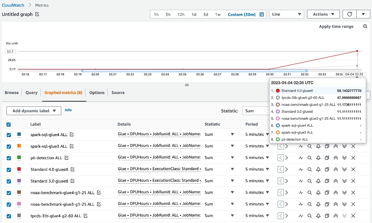
Each datapoint represents DPUHours per individual job run, so valid statistics for the CloudWatch metrics is SUM. With the CloudWatch metrics, you can have a granular view on DPU hours.
Options to optimize cost
This section describes key options to optimize costs on AWS Glue for Apache Spark:
- Upgrade to the latest version
- Auto scaling
- Flex
- Set the job’s timeout period appropriately
- Interactive sessions
- Smaller worker type for streaming jobs
We dive deep to the individual options.
Upgrade to the latest version
Having AWS Glue jobs running on the latest version enables you to take advantage of the latest functionalities and improvements offered by AWS Glue and the upgraded version of the supported engines such as Apache Spark. For example, AWS Glue 4.0 includes the new optimized Apache Spark 3.3.0 runtime and adds support for built-in pandas APIs as well as native support for Apache Hudi, Apache Iceberg, and Delta Lake formats, giving you more options for analyzing and storing your data. It also includes a new highly performant Amazon Redshift connector that is 10 times faster on TPC-DS benchmarking.
Auto scaling
One of the most common challenges to reduce cost is to identify the right amount of resources to run jobs. Users tend to overprovision workers in order to avoid resource-related problems, but part of those DPUs are not used, which increases costs unnecessarily. Starting with AWS Glue version 3.0, AWS Glue auto scaling helps you dynamically scale resources up and down based on the workload, for both batch and streaming jobs. Auto scaling reduces the need to optimize the number of workers to avoid over-provisioning resources for jobs, or paying for idle workers.
To enable auto scaling on AWS Glue Studio, go to the Job Details tab of your AWS Glue job and select Automatically scale number of workers.

You can learn more in Introducing AWS Glue Auto Scaling: Automatically resize serverless computing resources for lower cost with optimized Apache Spark.
Flex
For non-urgent data integration workloads that don’t require fast job start times or can afford to rerun the jobs in case of a failure, Flex could be a good option. The start times and runtimes of jobs using Flex vary because spare compute resources aren’t always available instantly and may be reclaimed during the run of a job. Flex-based jobs offer the same capabilities, including access to custom connectors, a visual job authoring experience, and a job scheduling system. With the Flex option, you can optimize the costs of your data integration workloads by up to 34%.
To enable Flex on AWS Glue Studio, go to the Job Details tab of your job and select Flex execution.

You can learn more in Introducing AWS Glue Flex jobs: Cost savings on ETL workloads.
Interactive sessions
One common practice among developers that create AWS Glue jobs is to run the same job several times every time a modification is made to the code. However, this may not be cost-effective depending of the number of workers assigned to the job and the number of times that it’s run. Also, this approach may slow down the development time because you have to wait until every job run is complete. To address this issue, in 2022 we released AWS Glue interactive sessions. This feature let developers process data interactively using a Jupyter-based notebook or IDE of their choice. Sessions start in seconds and have built-in cost management. As with AWS Glue jobs, you pay for only the resources you use. Interactive sessions allow developers to test their code line by line without needing to run the entire job to test any changes made to the code.
Set the job’s timeout period appropriately
Due to configuration issues, script coding errors, or data anomalies, sometimes AWS Glue jobs can take an exceptionally long time or struggle to process the data, and it can cause unexpected charges. AWS Glue gives you the ability to set a timeout value on any jobs. By default, an AWS Glue job is configured with 48 hours as the timeout value, but you can specify any timeout. We recommend identifying the average runtime of your job, and based on that, set an appropriate timeout period. This way, you can control cost per job run, prevent unexpected charges, and detect any problems related to the job earlier.
To change the timeout value on AWS Glue Studio, go to the Job Details tab of your job and enter a value for Job timeout.

Interactive sessions also have the same ability to set an idle timeout value on sessions. The default idle timeout value for Spark ETL sessions is 2880 minutes (48 hours). To change the timeout value, you can use %idle\_timeout magic.
Smaller worker type for streaming jobs
Processing data in real time is a common use case for customers, but sometimes these streams have sporadic and low data volumes. G.1X and G.2X worker types could be too big for these workloads, especially if we consider streaming jobs may need to run 24/7. To help you reduce costs, in 2022 we released G.025X, a new quarter DPU worker type for streaming ETL jobs. With this new worker type, you can process low data volume streams at one-fourth of the cost.
To select the G.025X worker type on AWS Glue Studio, go to the Job Details tab of your job. For Type, choose Spark Streaming, then choose G 0.25X for Worker type.
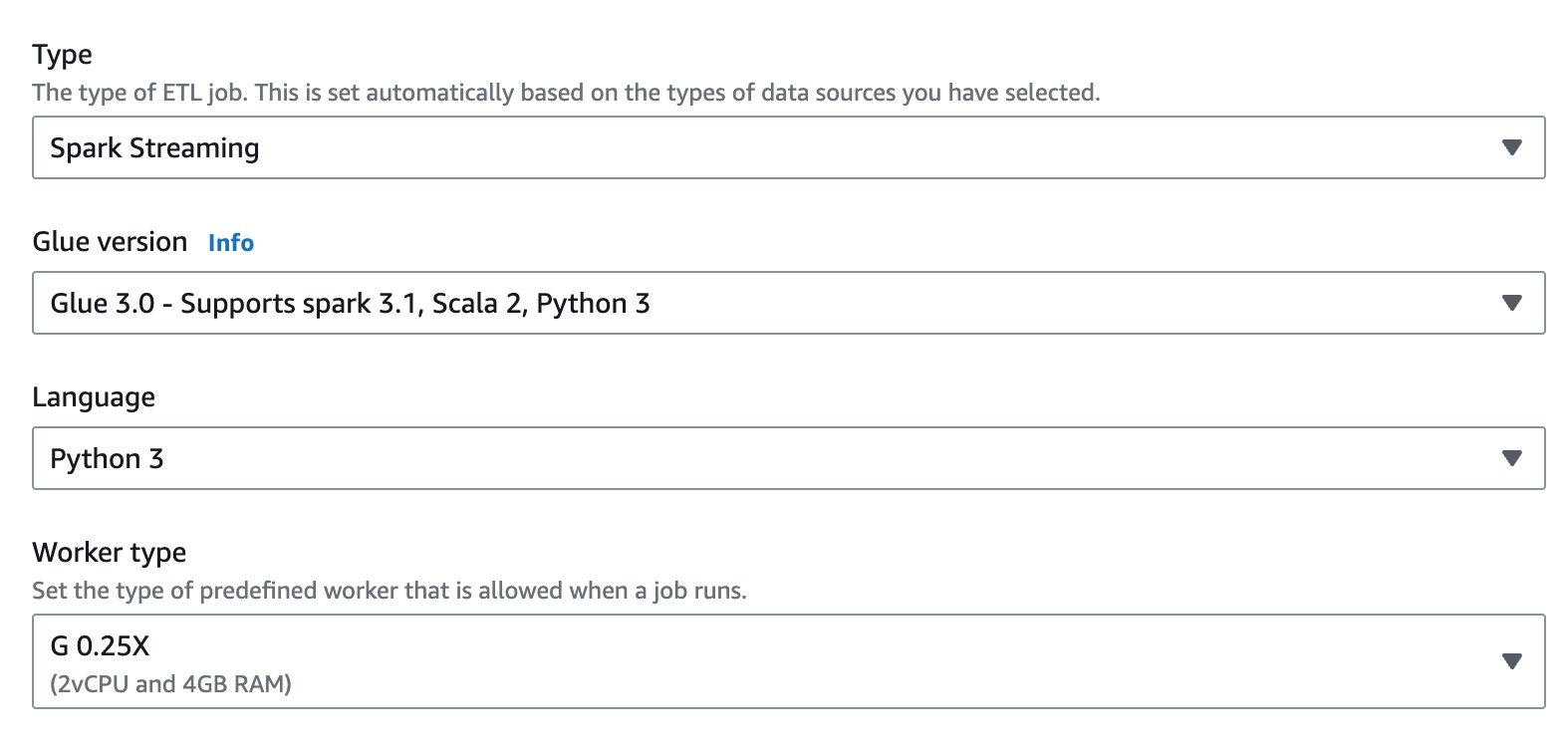
You can learn more in Best practices to optimize cost and performance for AWS Glue streaming ETL jobs.
Performance tuning to optimize cost
Performance tuning plays an important role in reducing cost. The first action for performance tuning is to identify the bottlenecks. Without measuring the performance and identifying bottlenecks, it’s not realistic to optimize cost-effectively. CloudWatch metrics provide a simple view for quick analysis, and the Spark UI provides deeper view for performance tuning. It’s highly recommended to enable Spark UI for your jobs and then view the UI to identify the bottleneck.
The following are high-level strategies to optimize costs:
- Scale cluster capacity
- Reduce the amount of data scanned
- Parallelize tasks
- Optimize shuffles
- Overcome data skew
- Accelerate query planning
For this post, we discuss the techniques for reducing the amount of data scanned and parallelizing tasks.
Reduce the amount of data scanned: Enable job bookmarks
AWS Glue job bookmarks are a capability to process data incrementally when running a job multiple times on a scheduled interval. If your use case is an incremental data load, you can enable job bookmarks to avoid a full scan for all job runs and process only the delta from the last job run. This reduces the amount of data scanned and accelerates individual job runs.
Reduce the amount of data scanned: Partition pruning
If your input data is partitioned in advance, you can reduce the amount of data scan by pruning partitions.
For AWS Glue DynamicFrame, set push\_down\_predicate (and catalogPartitionPredicate), as shown in the following code. Learn more in Managing partitions for ETL output in AWS Glue.
For Spark DataFrame (or Spark SQL), set a where or filter clause to prune partitions:
Parallelize tasks: Parallelize JDBC reads
The number of concurrent reads from the JDBC source is determined by configuration. Note that by default, a single JDBC connection will read all the data from the source through a SELECT query.
Both AWS Glue DynamicFrame and Spark DataFrame support parallelize data scans across multiple tasks by splitting the dataset.
For AWS Glue DynamicFrame, set hashfield or hashexpression and hashpartition. Learn more in Reading from JDBC tables in parallel.
For Spark DataFrame, set numPartitions, partitionColumn, lowerBound, and upperBound. Learn more in JDBC To Other Databases.
Conclusion
In this post, we discussed methodologies for monitoring and optimizing cost on AWS Glue for Apache Spark. With these techniques, you can effectively monitor and optimize costs on AWS Glue for Spark.
If you have comments or feedback, please leave them in the comments.
About the Authors
 Leonardo Gómez is a Principal Analytics Specialist Solutions Architect at AWS. He has over a decade of experience in data management, helping customers around the globe address their business and technical needs. Connect with him on LinkedIn
Noritaka Sekiyama is a Principal Big Data Architect on the AWS Glue team. He is responsible for building software artifacts to help customers. In his spare time, he enjoys cycling with his new road bike.
Amazon OpenSearch Ingestion is a serverless, auto-scaled, managed data collector that receives, transforms, and delivers data to Amazon OpenSearch Service domains or Amazon OpenSearch Serverless collections. OpenSearch Ingestion is powered by Data Prepper, an open-source, streaming ETL (extract, transform, and load) solution that’s part of the OpenSearch project. When you use OpenSearch Ingestion, you don’t need to maintain self-managed data pipelines to ingest logs, traces, metrics, and other data with OpenSearch Service. Amazon OpenSearch Ingestion responds to changing volumes of data, automatically scaling your ingest pipeline.
Distributed tracing is the leading way to locate, alert on, and remediate problems with your application and infrastructure. Distributed tracing is part of a broader observability solution, often combined with metrics and log data. OpenSearch Service gives you a native toolset to store and analyze large volumes of log, metric, and trace data. However, moving these large volumes of data is non-trivial to set up, monitor, and maintain.
In this post, we outline steps to set up a trace pipeline and strategies to deal with high volume tracing with Amazon OpenSearch Ingestion.
Solution overview
There is now a new option on the OpenSearch Service console called Pipelines under Ingestion in the navigation pane. We use this feature to create a trace pipeline.

You can also use the AWS Command Line Interface (AWS CLI), AWS CloudFormation, or AWS APIs to create a trace pipeline.
Prerequisites
Refer to Security in OpenSearch Ingestion to set up the permissions you need to create a pipeline and write to a pipeline, and the permissions the pipeline needs to write to a sink.
Create a trace pipeline
To create a trace pipeline, complete the following steps:
- On the OpenSearch Service console, choose Pipelines under Ingestion in the navigation pane.
- Choose Create pipeline.

Amazon OpenSearch Ingestion, powered by Data Prepper, uses pipelines as a mechanism to move the data from a source to a sink, with optional processors to mutate, route, sample, and detect anomalies for the data in the pipe. For more information, refer to Data Prepper. When you use Data Prepper, you build a YAML configuration file. When you use OpenSearch Ingestion, you upload your YAML configuration to the service. If you’re using the OpenSearch Service console, you can use one of the configuration blueprints that we provide. For distributed tracing, you will use an otel\_trace\_source and an OpenSearch Service domain as the sink.
- On the Configuration blueprints menu, choose AWS-TraceAnalyticsPipeline.

Choosing this blueprint will create a sample pipeline with otel\_trace\_source, an OpenSearch sink, along with span-pipeline and service-map-pipeline.
- Enter a name for this pipeline along with a minimum (1) and maximum (96) capacity value for Ingestion-OCUs.
Amazon OpenSearch Ingestion will scale automatically between these values to suit the volume of data you are ingesting.
- Edit the configuration’s
hosts,aws.sts\_role\_arn, andregionfields of the OpenSearch Service sink. - Follow rest of the steps to complete the trace pipeline creation.
Sample trace pipeline
The following code shows the components of a sample trace pipeline:
The sample trace pipeline has three sub-pipelines in its configuration. These are entry-pipeline, span-pipeline, and service-map-pipeline. The following diagram illustrates the workflow.
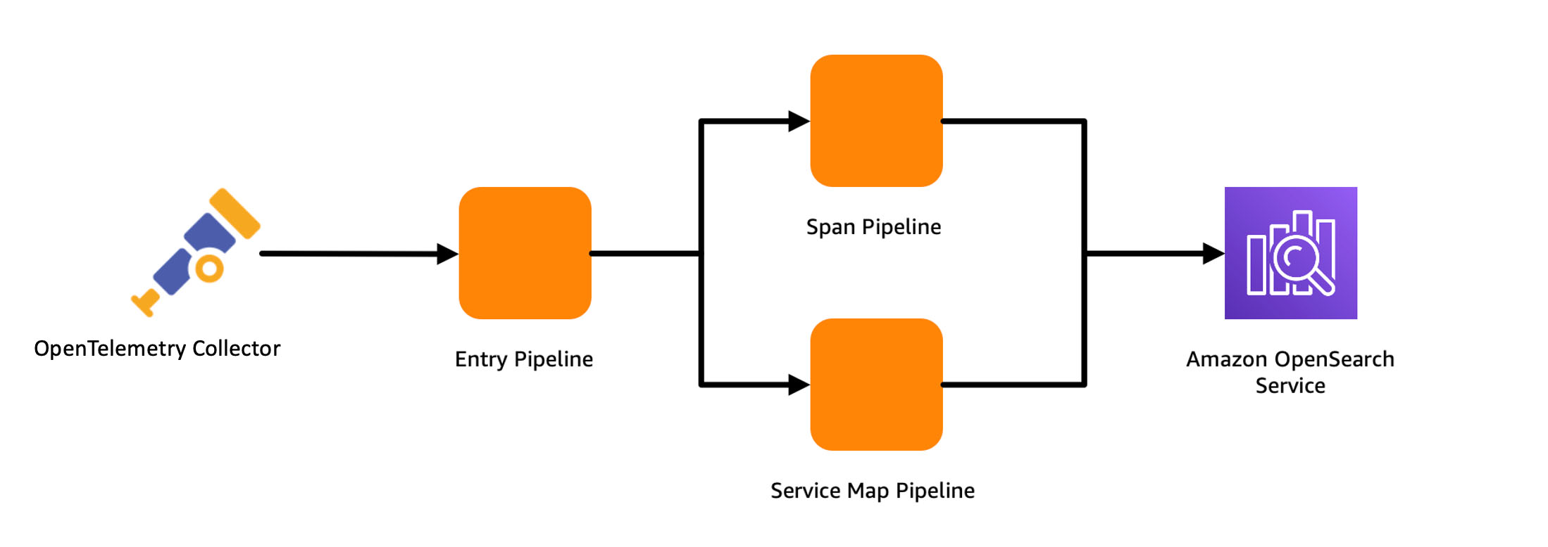
entry-pipeline specifies the source of data as otel\_trace\_source, which creates an HTTP listener for receiving OpenTelemetry traces at the ingestion URL for the pipeline. You use a trace\_peer\_forwarder processor to eliminate duplicate HTTP requests and forward the data to the span-pipeline and service-map pipelines. span-pipeline gets the raw trace data from entry-pipeline and uses the otel\_trace\_raw processor to complete trace group-related fields for the incoming span records. You use the service\_map\_stateful processor to have Data Prepper create the distributed service map for visualization in OpenSearch Dashboards. After the sample trace pipeline is created, it’s ready to receive OpenTelemetry traces at its ingestion URL!
Reduce your storage footprint and optimize for cost
The volume of traces collected from instrumenting a modern production enterprise application can reach tens or hundreds of terabytes very quickly, especially when you store every trace from every request. The problem of managing the storage footprint becomes important. In this section, we discuss strategies for reducing your storage footprint and optimizing for cost.
Use storage tiering
OpenSearch Service has three storage tiers: hot, UltraWarm, and cold. You use the hot tier to store frequently accessed data for quick reading and writing, the UltraWarm tier for infrequently used, read-only data backed by Amazon Simple Storage Service (Amazon S3) for lower cost, and the cold tier to maintain re-attachable data at near-Amazon S3 cost. By adjusting relative retention periods between these tiers, you can store a high volume of traces. For example, instead of storing 1 weeks’ worth of traces in the hot tier, you can store 2 days of traces in the hot tier and 15 days in the UltraWarm tier.
Extract metrics without storing traces
You can also use Data Prepper’s aggregation process to extract metrics in the pipeline to avoid delivering all of your data to OpenSearch Service. For example, you may want to analyze request, error, and duration (RED) metrics of your traces to know the current state of your services. OpenSearch Ingestion can calculate these metrics in the pipeline, aggregating them and storing them in separate indexes for analysis, reducing the ingestion and storage footprint of your traces. The following pipeline configuration snippet shows how to use the aggregate processor to calculate a histogram of the duration metric:
Use sampling
When your application is running without issues, the proportion of error traces is just a small percentage of your overall trace volume. Storing all of the traces for successful requests increases the cost substantially, while offering low value. To reduce cost, you can sample your trace data, reducing the number of traces you store in OpenSearch Service. There are generally two techniques for sampling:
- Head sampling – When you do head sampling, you ask OpenSearch Ingestion to make a sampling decision without looking at the whole trace. Head sampling is easy to configure and is efficient, but has a downside of possibly missing important traces.
- Tail sampling – Tail sampling is where you analyze the entirety of the trace and then decide whether to sample the trace or not. This accurately captures all the needed traces at the cost of complexity in configuring and implementing.
The following configuration snippet shows an example of the percent\_sampler, from the aggregate processor. In this example, you send only 25% of your traces to OpenSearch Service, based on head sampling:
Use conditional routing with sampling
Head sampling using the percentage\_sampler is simple and straightforward, but is a blunt tool. A better way to sample would be to gather, for example, 10% of successful responses, and 100% of failed responses or 100% high duration traces. To solve this, use conditional routing. Routes define conditions that can be used within processors and sinks to direct the data flowing through different parts of pipeline. For example, the following configuration snippet routes traces whose status code indicates a failure to the error\_trace pipeline. You forward 100% of the data in that pipe. You route traces whose duration metric is more than 1 second to the high\_latency pipeline where you sample them at 80%. Other normal traces are only sampled at 20%.
Conclusion
In this post, you learned how to configure an OpenSearch Ingestion pipeline and several strategies to keep in mind that help minimize cost while supporting a large-scale production system for distributed tracing. As next step, refer to the Amazon OpenSearch Developer Guide to explore logs and metric pipelines that you can use to build a scalable observability solution for your enterprise applications.
About the author
 Muthu Pitchaimani is a Search Specialist with Amazon OpenSearch Service. He builds large-scale search applications and solutions. Muthu is interested in the topics of networking and security, and is based out of Austin, Texas.
Amazon Athena supports the MERGE command on Apache Iceberg tables, which allows you to perform inserts, updates, and deletes in your data lake at scale using familiar SQL statements that are compliant with ACID (Atomic, Consistent, Isolated, Durable). Apache Iceberg is an open table format for data lakes that manages large collections of files as tables. It supports modern analytical data lake operations such as create table as select (CTAS), upsert and merge, and time travel queries. Athena also supports the ability to create views and perform VACUUM (snapshot expiration) on Apache Iceberg tables to optimize storage and performance. With these features, you can now build data pipelines completely in standard SQL that are serverless, more simple to build, and able to operate at scale. This enables developers to:
- Focus on writing business logic and not worry about setting up and managing the underlying infrastructure
- Perform data transformations with Athena
- Help comply with certain data deletion requirements
- Apply change data capture (CDC) from sources databases
With data lakes, data pipelines are typically configured to write data into a raw zone, which is an Amazon Simple Storage Service (Amazon S3) bucket or folder that contains data as is from source systems. Data is accumulated in this zone, such that inserts, updates, or deletes on the sources database appear as records in new files as transactions occur on the source. Although the raw zone can be queried, any downstream processing or analytical queries typically need to deduplicate data to derive a current view of the source table. For example, if a single record is updated multiple times in the source database, these be need to be deduplicated and the most recent record selected.
Typically, data transformation processes are used to perform this operation, and a final consistent view is stored in an S3 bucket or folder. Data transformation processes can be complex requiring more coding, more testing and are also error prone. This was a challenge because data lakes are based on files and have been optimized for appending data. Previously, you had to overwrite the complete S3 object or folder, which was not only inefficient but also interrupted users who were querying the same data. With the evolution of frameworks such as Apache Iceberg, you can perform SQL-based upsert in-place in Amazon S3 using Athena, without blocking user queries and while still maintaining query performance.
In this post, we demonstrate how you can use Athena to apply CDC from a relational database to target tables in an S3 data lake.
Overview of solution
For this post, consider a mock sports ticketing application based on the following project. We use a single table in that database that contains sporting events information and ingest it into an S3 data lake on a continuous basis (initial load and ongoing changes). This data ingestion pipeline can be implemented using AWS Database Migration Service (AWS DMS) to extract both full and ongoing CDC extracts. With CDC, you can determine and track data that has changed and provide it as a stream of changes that a downstream application can consume. Most databases use a transaction log to record changes made to the database. AWS DMS reads the transaction log by using engine-specific API operations and captures the changes made to the database in a nonintrusive manner.
Specifically, to extract changed data including inserts, updates, and deletes from the database, you can configure AWS DMS with two replication tasks, as described in the following workshop. The first task performs an initial copy of the full data into an S3 folder. The second task is configured to replicate ongoing CDC into a separate folder in S3, which is further organized into date-based subfolders based on the source databases’ transaction commit date. With full and CDC data in separate S3 folders, it’s easier to maintain and operate data replication and downstream processing jobs. To enable this, you can apply the following extra connection attributes to the S3 endpoint in AWS DMS, (refer to S3Settings for other CSV and related settings):
- TimestampColumnName – AWS DMS adds a column that you name with timestamp information for the commit of that row in the source database.
- includeOpForFullLoad – AWS DMS adds a column named Op to every file to indicate if the record is an I (INSERT), U (UPDATE), or D (DELETE).
- DatePartitionEnabled, DatePartitionSequence, DatePartitionDelimiter – These settings are used to configure AWS DMS to write changed data to date/time-based folders in the data lake. By partitioning folders, you can better manage S3 objects and optimize data lake queries for subsequent downstream processing.
We use the support in Athena for Apache Iceberg tables called MERGE INTO, which can express row-level updates. Apache Iceberg supports MERGE INTO by rewriting data files that contain rows that need to be updated. After the data is merged, we demonstrate how to use Athena to perform time travel on the sporting\_event table, and use views to abstract and present different versions of the data to end-users. Finally, to simplify table maintenance, we demonstrate performing VACUUM on Apache Iceberg tables to delete older snapshots, which will optimize latency and cost of both read and write operations.
The following diagram illustrates the solution architecture.
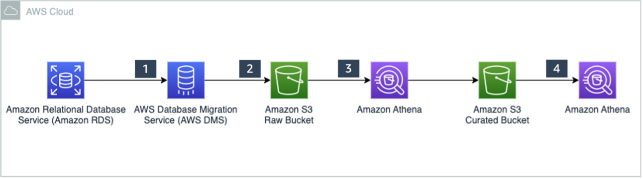
The solution workflow consists of the following steps:
- Data ingestion:
- Steps 1 and 2 use AWS DMS, which connects to the source database to load initial data and ongoing changes (CDC) to Amazon S3 in CSV format. For this post, we have provided sample full and CDC datasets in CSV format that have been generated using AWS DMS.
- Step 3 is comprised of the following actions:
- Create an external table in Athena pointing to the source data ingested in Amazon S3.
- Create an Apache Iceberg target table and load data from the source table.
- Merge CDC data into the Apache Iceberg table using MERGE INTO.
- Data access:
- In Step 4, create a view on the Apache Iceberg table.
- Use the view to query data using standard SQL.
Prerequisites
Before getting started, make sure you have the required permissions to perform the following in your AWS account:
- Create AWS Identity and Access Management (IAM) roles as needed
- Read and write to an S3 bucket
- Manage a database, table, and workgroups, and run queries in Athena
Create tables on the raw data
First, create a database for this demo.
- Navigate to the Athena console and choose Query editor.
If this is your first time using the Athena query editor, you need to configure and specify an S3 bucket to store the query results. - Create a database with the following code:
- Next, create a folder in an S3 bucket that you can use for this demo. Name this folder
sporting\_event\_full. - Upload LOAD00000001.csv into the folder.
- Switch to the
raw\_demodatabase and create a table to point to the raw input data: - Run the following query to review the data:

- Next, create another folder in the same S3 bucket called
sporting\_event\_cdc. - Within this folder, create three subfolders in a time hierarchy folder structure such that the final S3 folder URI looks like
s3://<your-bucket>/sporting\_event\_cdc/2022/09/22/. - Upload 20220922-184314489.csv into this folder.This folder structure is similar to how AWS DMS stores CDC data when you enable date-based folder partitioning.
- Create a table to point to the CDC data. This table also includes a partition column because the source data in Amazon S3 is organized into date-based folders.
- Next, alter the table to add new partitions. Because the data is stored in non-Hive style format by AWS DMS, to query this data, add this partition manually or use an AWS Glue crawler. As data accumulates, continue to add new partitions to query this data.
- Run the following query to review the CDC data:
There are two records with IDs 1 and 11 that are updates with op code U. The record with ID 21 has a delete (D) op code, and the record with ID 5 is an insert (I).
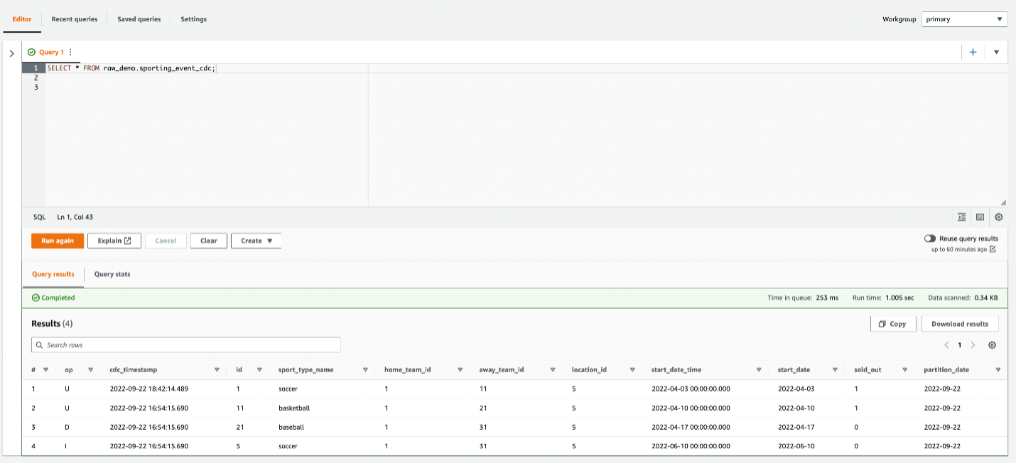
Use CTAS to create the target Iceberg table in Parquet format
CTAS statements create new tables using standard SELECT queries. The resultant table is added to the AWS Glue Data Catalog and made available for querying.
- First, create another database to store the target table:
- Next, switch to this database and run the CTAS statement to select data from the raw input table to create the target Iceberg table (replace the location with an appropriate S3 bucket in your account):
- Run the following query to review data in the Iceberg table:
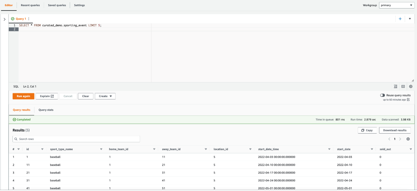
Use MERGE INTO to insert, update, and delete data into the Iceberg table
The MERGE INTO command updates the target table with data from the CDC table. The following statement uses a combination of primary keys and the Op column in the source data, which indicates if the source row is an insert, update, or delete. We use the id column as the primary key to join the target table to the source table, and we use the Op column to determine if a record needs to be deleted.
Run the following query to verify data in the Iceberg table:
The record with ID 21 has been deleted, and the other records in the CDC dataset have been updated and inserted, as expected.

Create a view that contains the previous state
When you write to an Iceberg table, a new snapshot or version of a table is created each time.
A snapshot represents the state of a table at a point in time and is used to access the complete set of data files in the table. Time travel queries in Athena query Amazon S3 for historical data from a consistent snapshot as of a specified date and time or a specified snapshot ID. However, this requires knowledge of a table’s current snapshots. To abstract this information from users, you can create views on top of Iceberg tables:
Run the following query using this view to retrieve the snapshot of data before the CDC was applied:
You can see the record with ID 21, which was deleted earlier.
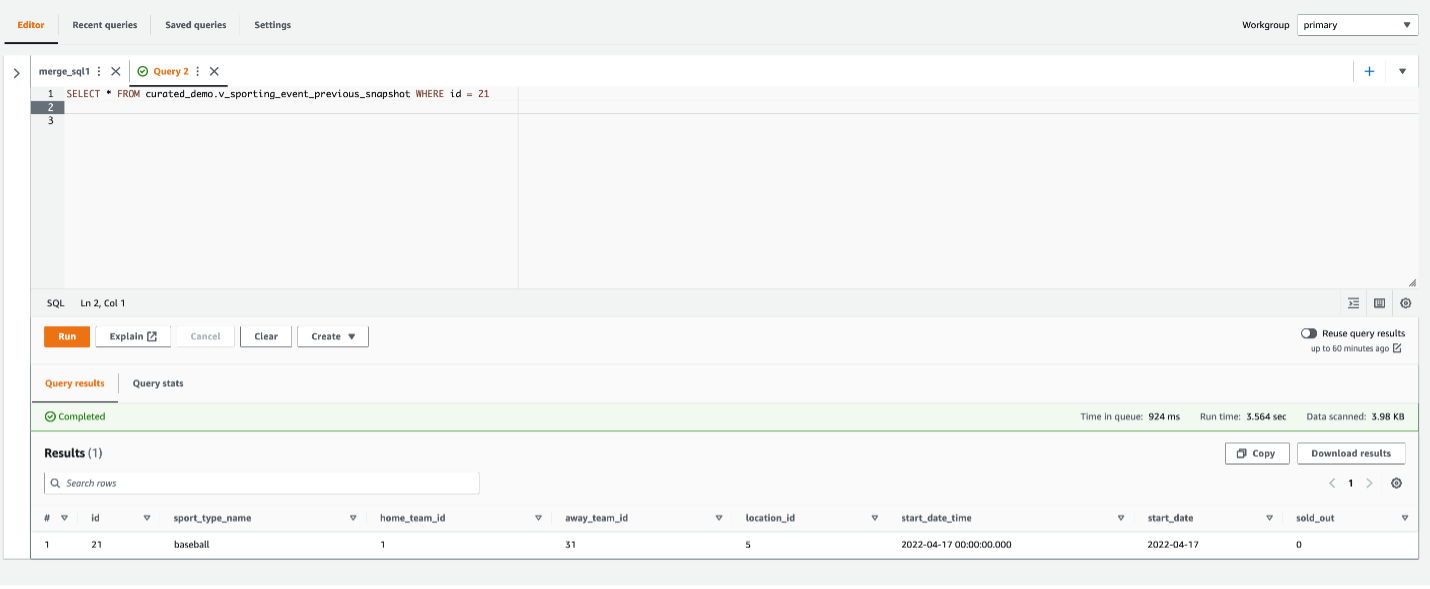
Compliance with privacy regulations may require that you permanently delete records in all snapshots. To accomplish this, you can set properties for snapshot retention in Athena when creating the table, or you can alter the table:
This instructs Athena to store only one version of the data and not maintain any transaction history. After a table has been updated with these properties, run the VACUUM command to remove the older snapshots and clean up storage:
Run the following query again:
The record with ID 21 has been permanently deleted.
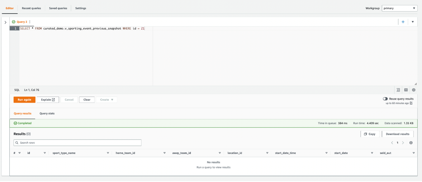
Considerations
As data accumulates in the CDC folder of your raw zone, older files can be archived to Amazon S3 Glacier. Subsequently, the MERGE INTO statement can also be run on a single source file if needed by using $path in the WHERE condition of the USING clause:
This results in Athena scanning all files in the partition’s folder before the filter is applied, but can be minimized by choosing fine-grained hourly partitions. With this approach, you can trigger the MERGE INTO to run on Athena as files arrive in your S3 bucket using Amazon S3 event notifications. This could enable near-real-time use cases where users need to query a consistent view of data in the data lake as soon it is created in source systems.
Clean up
To avoid incurring ongoing costs, complete the following steps to clean up your resources:
- Run the following SQL to drop the tables and views:
Because Iceberg tables are considered managed tables in Athena, dropping an Iceberg table also removes all the data in the corresponding S3 folder.
- Run the following SQL to drop the databases:
- Delete the S3 folders and CSV files that you had uploaded.
Conclusion
This post showed you how to apply CDC to a target Iceberg table using CTAS and MERGE INTO statements in Athena. You can perform bulk load using a CTAS statement. When new data or changed data arrives, use the MERGE INTO statement to merge the CDC changes. To optimize storage and improve performance of queries, use the VACUUM command regularly.
As next steps, you can orchestrate these SQL statements using AWS Step Functions to implement end-to-end data pipelines for your data lake. For more information, refer to Build and orchestrate ETL pipelines using Amazon Athena and AWS Step Functions.
About the Authors
Ranjit Rajan is a Principal Data Lab Solutions Architect with AWS. Ranjit works with AWS customers to help them design and build data and analytics applications in the cloud.
 Kannan Iyer is a Senior Data Lab Solutions Architect with AWS. Kannan works with AWS customers to help them design and build data and analytics applications in the cloud.
 Alexandre Rezende is a Data Lab Solutions Architect with AWS. Alexandre works with customers on their Business Intelligence, Data Warehouse, and Data Lake use cases, design architectures to solve their business problems, and helps them build MVPs to accelerate their path to production.
Amazon OpenSearch Service is a managed service that makes it easy to secure, deploy, and operate OpenSearch and legacy Elasticsearch clusters at scale in the AWS Cloud. Amazon OpenSearch Service provisions all the resources for your cluster, launches it, and automatically detects and replaces failed nodes, reducing the overhead of self-managed infrastructures. The service makes it easy for you to perform interactive log analytics, real-time application monitoring, website searches, and more by offering the latest versions of OpenSearch, support for 19 versions of Elasticsearch (1.5 to 7.10 versions), and visualization capabilities powered by OpenSearch Dashboards and Kibana (1.5 to 7.10 versions). Amazon OpenSearch Service now offers a serverless deployment option (public preview) that makes it even easier to use OpenSearch in the AWS cloud.
A typical workflow for OpenSearch is to store documents (as JSON data) in an index, and execute searches (also JSON) to find those documents. Percolation reverses that. You store searches and query with documents. Let’s say I’m searching for a house in Chicago that costs < 500K. I could go to the website every day and run my query. A clever website would be able to store my requirements (a query) and notify me when something new (a document) comes up that matches my requirements. Percolation is an OpenSearch feature that enables the website to store these queries and run documents against them to find new matches.
In this post, We will explore how to use percolators to find matching homes from new listings.
Before getting into the details of percolators, let’s explore how search works. When you insert a document, OpenSearch maintains an internal data structure called the “inverted index” which speeds up the search.
Indexing and Searching:
Let’s take the above example of a real estate application having the simple schema of type of the house, city, and the price.
- First, let’s create an index with mappings as below
- Let’s insert some documents into the index.
| ID | House\_type | City | Price |
| 1 | townhouse | Chicago | 650000 |
| 2 | house | Washington | 420000 |
| 3 | condo | Chicago | 580000 |
- As we don’t have any townhouses listed in Chicago for less than 500K, the below query returns no results.
If you’re curious to know how search works under the hood at high level, you can refer to this article.
Percolation:
If one of your customers wants to get notified when a townhouse in Chicago is available, and listed at less than $500,000, you can store their requirements as a query in the percolator index. When a new listing becomes available, you can run that listing against the percolator index with a \_percolate query. The query will return all matches (each match is a single set of requirements from one user) for that new listing. You can then notify each user that a new listing is available that fits their requirements. This process is called percolation in OpenSearch.
OpenSearch has a dedicated data type called “percolator” that allows you to store queries.
Let’s create a percolator index with the same mapping, with additional fields for query and optional metadata. Make sure you include all the necessary fields that are part of a stored query. In our case, along with the actual fields and query, we capture the customer\_id and priority to send notifications.
After creating the index, insert a query as below
The percolation begins when a new document gets run against the stored queries.
Run the percolation query with document(s), and it matches the stored query
The above query returns the queries along with the metadata we stored (customer\_id in our case) that matches the documents
Percolation at scale
When you have a high volume of queries stored in the percolator index, searching queries across the index might be inefficient. You can consider segmenting your queries and use them as filters to handle the high-volume queries effectively. As we already capture priority, you can now run percolation with filters on priority that reduces the scope of matching queries.
Best practices
- Prefer the percolation index separate from the document index. Different index configurations, like number of shards on percolation index, can be tuned independently for performance.
- Prefer using query filters to reduce matching queries to percolate from percolation index.
- Consider using a buffer in your ingestion pipeline for reasons below,
- You can batch the ingestion and percolation independently to suit your workload and SLA
- You can prioritize the ingest and search traffic by running the percolation at off hours. Make sure that you have enough storage in the buffering layer.

- Consider using an independent cluster for percolation for the below reasons,
-
- The percolation process relies on memory and compute, your primary search will not be impacted.
- You have the flexibility of scaling the clusters independently.

Conclusion
In this post, we walked through how percolation in OpenSearch works, and how to use effectively, at scale. Percolation works in both managed and serverless versions of OpenSearch. You can follow the best practices to analyze and arrange data in an index, as it is important for a snappy search performance.
If you have feedback about this post, submit your comments in the comments section.
About the author
 Arun Lakshmanan is a Search Specialist with Amazon OpenSearch Service based out of Chicago, IL. He has over 20 years of experience working with enterprise customers and startups. He loves to travel and spend quality time with his family.
This is a guest post co-written by Maik Leuthold and Nick Harmening from BMW Group.
The BMW Group is headquartered in Munich, Germany, where the company oversees 149,000 employees and manufactures cars and motorcycles in over 30 production sites across 15 countries. This multinational production strategy follows an even more international and extensive supplier network.
Like many automobile companies across the world, the BMW Group has been facing challenges in its supply chain due to the worldwide semiconductor shortage. Creating transparency about BMW Group’s current and future demand of semiconductors is one key strategic aspect to resolve shortages together with suppliers and semiconductor manufacturers. The manufacturers need to know BMW Group’s exact current and future semiconductor volume information, which will effectively help steer the available worldwide supply.
The main requirement is to have an automated, transparent, and long-term semiconductor demand forecast. Additionally, this forecasting system needs to provide data enrichment steps including byproducts, serve as the master data around the semiconductor management, and enable further use cases at the BMW Group.
To enable this use case, we used the BMW Group’s cloud-native data platform called the Cloud Data Hub. In 2019, the BMW Group decided to re-architect and move its on-premises data lake to the AWS Cloud to enable data-driven innovation while scaling with the dynamic needs of the organization. The Cloud Data Hub processes and combines anonymized data from vehicle sensors and other sources across the enterprise to make it easily accessible for internal teams creating customer-facing and internal applications. To learn more about the Cloud Data Hub, refer to BMW Group Uses AWS-Based Data Lake to Unlock the Power of Data.
In this post, we share how the BMW Group analyzes semiconductor demand using AWS Glue.
Logic and systems behind the demand forecast
The first step towards the demand forecast is the identification of semiconductor-relevant components of a vehicle type. Each component is described by a unique part number, which serves as a key in all systems to identify this component. A component can be a headlight or a steering wheel, for example.
For historic reasons, the required data for this aggregation step is siloed and represented differently in diverse systems. Because each source system and data type have its own schema and format, it’s particularly difficult to perform analytics based on this data. Some source systems are already available in the Cloud Data Hub (for example, part master data), therefore it’s straightforward to consume from our AWS account. To access the remaining data sources, we need to build specific ingest jobs that read data from the respective system.
The following diagram illustrates the approach.
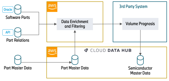
The data enrichment starts with an Oracle Database (Software Parts) that contains part numbers that are related to software. This can be the control unit of a headlight or a camera system for automated driving. Because semiconductors are the basis for running software, this database builds the foundation of our data processing.
In the next step, we use REST APIs (Part Relations) to enrich the data with further attributes. This includes how parts are related (for example, a specific control unit that will be installed into a headlight) and over which timespan a part number will be built into a vehicle. The knowledge about the part relations is essential to understand how a specific semiconductor, in this case the control unit, is relevant for a more general part, the headlight. The temporal information about the use of part numbers allows us to filter out outdated part numbers, which will not be used in the future and therefore have no relevance in the forecast.
The data (Part Master Data) can directly be consumed from the Cloud Data Hub. This database includes attributes about the status and material types of a part number. This information is required to filter out part numbers that we gathered in the previous steps but have no relevance for semiconductors. With the information that was gathered from the APIs, this data is also queried to extract further part numbers that weren’t ingested in the previous steps.
After data enrichment and filtering, a third-party system reads the filtered part data and enriches the semiconductor information. Subsequently, it adds the volume information of the components. Finally, it provides the overall semiconductor demand forecast centrally to the Cloud Data Hub.
Applied services
Our solution uses the serverless services AWS Glue and Amazon Simple Storage Service (Amazon S3) to run ETL (extract, transform, and load) workflows without managing an infrastructure. It also reduces the costs by paying only for the time jobs are running. The serverless approach fits our workflow’s schedule very well because we run the workload only once a week.
Because we’re using diverse data source systems as well as complex processing and aggregation, it’s important to decouple ETL jobs. This allows us to process each data source independently. We also split the data transformation into several modules (Data Aggregation, Data Filtering, and Data Preparation) to make the system more transparent and easier to maintain. This approach also helps in case of extending or modifying existing jobs.
Although each module is specific to a data source or a particular data transformation, we utilize reusable blocks inside of every job. This allows us to unify each type of operation and simplifies the procedure of adding new data sources and transformation steps in the future.
In our setup, we follow the security best practice of the least privilege principle, to ensure the information is protected from accidental or unnecessary access. Therefore, each module has AWS Identity and Access Management (IAM) roles with only the necessary permissions, namely access to only data sources and buckets the job deals with. For more information regarding security best practices, refer to Security best practices in IAM.
Solution overview
The following diagram shows the overall workflow where several AWS Glue jobs are interacting with each other sequentially.

As we mentioned earlier, we used the Cloud Data Hub, Oracle DB, and other data sources that we communicate with via the REST API. The first step of the solution is the Data Source Ingest module, which ingests the data from different data sources. For that purpose, AWS Glue jobs read information from different data sources and writes into the S3 source buckets. Ingested data is stored in the encrypted buckets, and keys are managed by AWS Key Management Service (AWS KMS).
After the Data Source Ingest step, intermediate jobs aggregate and enrich the tables with other data sources like components version and categories, model manufacture dates, and so on. Then they write them into the intermediate buckets in the Data Aggregation module, creating comprehensive and abundant data representation. Additionally, according to the business logic workflow, the Data Filtering and Data Preparation modules create the final master data table with only actual and production-relevant information.
The AWS Glue workflow manages all these ingestion jobs and filtering jobs end to end. An AWS Glue workflow schedule is configured weekly to run the workflow on Wednesdays. While the workflow is running, each job writes execution logs (info or error) into Amazon Simple Notification Service (Amazon SNS) and Amazon CloudWatch for monitoring purposes. Amazon SNS forwards the execution results to the monitoring tools, such as Mail, Teams, or Slack channels. In case of any error in the jobs, Amazon SNS also alerts the listeners about the job execution result to take action.
As the last step of the solution, the third-party system reads the master table from the prepared data bucket via Amazon Athena. After further data engineering steps like semiconductor information enrichment and volume information integration, the final master data asset is written into the Cloud Data Hub. With the data now provided in the Cloud Data Hub, other use cases can use this semiconductor master data without building several interfaces to different source systems.
Business outcome
The project results provide the BMW Group a substantial transparency about their semiconductor demand for their entire vehicle portfolio in the present and in the future. The creation of a database with that magnitude enables the BMW Group to establish even further use cases to the benefit of more supply chain transparency and clearer and deeper exchange with first-tier suppliers and semiconductor manufacturers. It helps not only to resolve the current demanding market situation, but also to be more resilient in the future. Therefore, it’s one major step to a digital, transparent supply chain.
Conclusion
This post describes how to analyze semiconductor demand from many data sources with big data jobs in an AWS Glue workflow. A serverless architecture with minimal diversity of services makes the code base and architecture simple to understand and maintain. To learn more about how to use AWS Glue workflows and jobs for serverless orchestration, visit the AWS Glue service page.
About the authors
 Maik Leuthold is a Project Lead at the BMW Group for advanced analytics in the business field of supply chain and procurement, and leads the digitalization strategy for the semiconductor management.
 Nick Harmening is an IT Project Lead at the BMW Group and an AWS certified Solutions Architect. He builds and operates cloud-native applications with a focus on data engineering and machine learning.
 Göksel Sarikaya is a Senior Cloud Application Architect at AWS Professional Services. He enables customers to design scalable, cost-effective, and competitive applications through the innovative production of the AWS platform. He helps them to accelerate customer and partner business outcomes during their digital transformation journey.
 Alexander Tselikov is a Data Architect at AWS Professional Services who is passionate about helping customers to build scalable data, analytics and ML solutions to enable timely insights and make critical business decisions.
 Rahul Shaurya is a Senior Big Data Architect at Amazon Web Services. He helps and works closely with customers building data platforms and analytical applications on AWS. Outside of work, Rahul loves taking long walks with his dog Barney.
This is a guest blog post co-written with Corey Johnson from Huron.
Having an accurate and up-to-date inventory of all technical assets helps an organization ensure it can keep track of all its resources with metadata information such as their assigned oners, last updated date, used by whom, how frequently and more. It helps engineers, analysts and businesses access the most up-to-date release of the software asset that bring accuracy to the decision-making process. By keeping track of this information, organizations will be able to identify technology gaps, refresh cycles, and expire assets as needed for archival.
In addition, an inventory of all assets is one of the foundational elements of an organization that facilitates the security and compliance team to audit the assets for improving privacy, security posture and mitigate risk to ensure the business operations run smoothly. Organizations may have different ways of maintaining an asset inventory, that may be an Excel spreadsheet or a database with a fully automated system to keep it up-to-date, but with a common objective of keeping it accurate. Even if organizations can follow manual approaches to update the inventory records but it is recommended to build automation, so that it is accurate at any point of time.
The DevOps practices which revolutionized software engineering in the last decade have yet to come to the world of Business Intelligence solutions. Business intelligence tools by their nature use a paradigm of UI driven development with code-first practices being secondary or nonexistent. As the need for applications that can leverage the organizations internal and client data increases, the same DevOps practices (BIOps) can drive and delivery quality insights more reliably
In this post, we walk you through a solution that Huron and manage lifecycle for all Amazon QuickSight resources across the organization by collaborating with AWS Data Lab Resident Architect & AWS Professional Services team.
About Huron
Huron is a global professional services firm that collaborates with clients to put possible into practice by creating sound strategies, optimizing operations, accelerating digital transformation, and empowering businesses and their people to own their future. By embracing diverse perspectives, encouraging new ideas, and challenging the status quo, Huron creates sustainable results for the organizations we serve. To help address its clients’ growing cloud needs, Huron is an AWS Partner.
Use Case Overview
Huron’s Business Intelligence use case represents visualizations as a service, where Huron has core set of visualizations and dashboards available as products for its customers. The products exist in different industry verticals (healthcare, education, commercial) with independent development teams. Huron’s consultants leverage the products to provide insights as part of consulting engagements. The insights from the product help Huron’s consultants accelerate their customer’s transformation. As part of its overall suite of offerings, there are product dashboards that are featured in a software application following a standardized development lifecycle. In addition, these product dashboards may be forked for customer-specific customization to support a consulting engagement while still consuming from Huron’s productized data assets and datasets. In the next stage of the cycle, Huron’s consultants experiment with new data sources and insights that in turn fed back into the product dashboards.
When changes are made to a product analysis, challenges arise when a base reference analysis gets updated because of new feature releases or bug fixes, and all the customer visualizations that are created from it also need to be updated. To maintain the integrity of embedded visualizations, all metadata and lineage must be available to the parent application. This access to the metadata supports the need for updating visuals based on changes as well as automating row and column level security ensuring customer data is properly governed.
In addition, few customers request customizations on top of the base visualizations, for which Huron team needs to create a replica of the base reference and then customize it for the customer. These are maintained by Huron’s in the field consultants rather than the product development team. These customer specific visualizations create operational overhead because they require Huron to keep track of new customer specific visualizations and maintain them for future releases when the product visuals change.
Huron leverages Amazon QuickSight for their Business Intelligence (BI) reporting needs, enabling them to embed visualizations at scale with higher efficiency and lower cost. A large attraction for Huron to adopt QuickSight came from the forward-looking API capabilities that enable and set the foundation for a BIOps culture and technical infrastructure. To address the above requirement, Huron Global Product team decided to build a QuickSight Asset Tracker and QuickSight Asset Deployment Pipeline.
The QuickSight Asset tracker serves as a catalogue of all QuickSight resources (datasets, analysis, templates, dashboards etc.) with its interdependent relationship. It will help;
- Create an inventory of all QuickSight resources across all business units
- Enable dynamic embedding of visualizations and dashboards based on logged in user
- Enable dynamic row and column level security on the dashboards and visualizations based on the logged-in user
- Meet compliance and audit requirements of the organization
- Maintain the current state of all customer specific QuickSight resources
The solution integrates an AWS CDK based pipeline to deploy QuickSight Assets that:
- Supports Infrastructure-as-a-code for QuickSight Asset Deployment and enables rollbacks if required.
- Enables separation of development, staging and production environments using QuickSight folders that reduces the burden of multi-account management of QuickSight resources.
- Enables a hub-and-spoke model for Data Access in multiple AWS accounts in a data mesh fashion.
QuickSight Asset Tracker and QuickSight Asset Management Pipeline – Architecture Overview
The QuickSight Asset Tracker was built as an independent service, which was deployed in a shared AWS service account that integrated Amazon Aurora Serverless PostgreSQL to store metadata information, AWS Lambda as the serverless compute and Amazon API Gateway to provide the REST API layer.
It also integrated AWS CDK and AWS CloudFormation to deploy the product and customer specific QuickSight resources and keep them in consistent and stable state. The metadata of QuickSight resources, created using either AWS console or the AWS CDK based deployment were maintained in Amazon Aurora database through the QuickSight Asset Tracker REST API service.
The CDK based deployment pipeline is triggered via a CI/CD pipeline which performs the following functions:
- Takes the ARN of the QuickSight assets (dataset, analysis, etc.)
- Describes the asset and dependent resources (if selected)
- Creates a copy of the resource in another environment (in this case a QuickSight folder) using CDK
The solution architecture integrated the following AWS services.
- Amazon Aurora Serverless integrated as the backend database to store metadata information of all QuickSight resources with customer and product information they are related to.
- Amazon QuickSight as the BI service using which visualization and dashboards can be created and embedded into the online applications.
- AWS Lambda as the serverless compute service that gets invoked by online applications using Amazon API Gateway service.
- Amazon SQS to store customer request messages, so that the AWS CDK based pipeline can read from it for processing.
- AWS CodeCommit is integrated to store the AWS CDK deployment scripts and AWS CodeBuild, AWS CloudFormation integrated to deploy the AWS resources using an infrastructure as a code approach.
- AWS CloudTrail is integrated to audit user actions and trigger Amazon EventBridge rules when a QuickSight resource is created, updated or deleted, so that the QuickSight Asset Tracker is up-to-date.
- Amazon S3 integrated to store metadata information, which is used by AWS CDK based pipeline to deploy the QuickSight resources.
- AWS LakeFormation enables cross-account data access in support of the QuickSight Data Mesh
The following provides a high-level view of the solution architecture.

Architecture Walkthrough:
The following provides a detailed walkthrough of the above architecture.
- QuickSight Dataset, Template, Analysis, Dashboard and visualization relationships:
- Steps 1 to 2 represent QuickSight reference analysis reading data from different data sources that may include Amazon S3, Amazon Athena, Amazon Redshift, Amazon Aurora or any other JDBC based sources.
- Step 3 represents QuickSight templates being created from reference analysis when a customer specific visualization needs to be created and step 4.1 to 4.2 represents customer analysis and dashboards being created from the templates.
- Steps 7 to 8 represent QuickSight visualizations getting generated from analysis/dashboard and step 6 represents the customer analysis/dashboard/visualizations referring their own customer datasets.
- Step 10 represents a new fork being created from the base reference analysis for a specific customer, which will create a new QuickSight template and reference analysis for that customer.
- Step 9 represents end users accessing QuickSight visualizations.
- Asset Tracker REST API service:
- Step 15.2 to 15.4 represents the Asset Tracker service, which is deployed in a shared AWS service account, where Amazon API Gateway provides the REST API layer, which invokes AWS Lambda function to read from or write to backend Aurora database (Aurora Serverless v2 – PostgreSQL engine). The database captures all relationship metadata between QuickSight resources, its owners, assigned customers and products.
- Online application – QuickSight asset discovery and creation
- Step 15.1 represents the front-end online application reading QuickSight metadata information from the Asset Tracker service to help customers or end users discover visualizations available and be able to dynamically render based on the user login.
- Step 11 to 12 represents the online application requesting creation of new QuickSight resources, which pushes requests to Amazon SQS and then AWS Lambda triggers AWS CodeBuild to deploy new QuickSight resources. Step 13.1 and 13.2 represents the CDK based pipeline maintaining the QuickSight resources to keep them in a consistent state. Finally, the AWS CDK stack invokes the Asset Tracker service to update its metadata as represented in step 13.3.
- Tracking QuickSight resources created outside of the AWS CDK Stack
- Step 14.1 represents users creating QuickSight resources using the AWS Console and step 14.2 represents that activity getting logged into AWS CloudTrail.
- Step 14.3 to 14.5 represents triggering EventBridge rule for CloudTrail activities that represents QuickSight resource being created, updated or deleted and then invoke the Asset Tracker REST API to register the QuickSight resource metadata.
Architecture Decisions:
The following are few architecture decisions we took while designing the solution.
- Choosing Aurora database for Asset Tracker: We have evaluated Amazon Neptune for the Asset Tracker database as most of the metadata information we capture are primarily maintaining relationship between QuickSight resources. But when we looked at the query patterns, we found the query pattern is always just one level deep to find who is the parent of a specific QuickSight resource and that can be solved with a relational database’s Primary Key / Foreign Key relationship and with simple self-join SQL query. Knowing the query pattern does not require a graph database, we decided to go with Amazon Aurora to keep it simple, so that we can avoid introducing a new database technology and can reduce operational overhead of maintaining it. In future as the use case evolve, we can evaluate the need for a Graph database and plan for integrating it. For Amazon Aurora, we choose Amazon Aurora Serverless as the usage pattern is not consistent to reserve a server capacity and the serverless tech stack will help reduce operational overhead.
- Decoupling Asset Tracker as a common REST API service: The Asset Tracker has future scope to be a centralized metadata layer to keep track of all the QuickSight resources across all business units of Huron. So instead of each business unit having its own metadata database, if we build it as a service and deploy it in a shared AWS service account, then we will get benefit from reduced operational overhead, duplicate infrastructure cost and will be able to get a consolidated view of all assets and their integrations. The service provides the ability of applications to consume metadata about the QuickSight assets and then apply their own mapping of security policies to the assets based on their own application data and access control policies.
- Central QuickSight account with subfolder for environments: The choice was made to use a central account which reduces developer friction of having multiple accounts with multiple identities, end users having to manage multiple accounts and access to resources. QuickSight folders allow for appropriate permissions for separating “environments”. Furthermore, by using folder-based sharing with QuickSight groups, users with appropriate permissions already have access to the latest versions of QuickSight assets without having to share their individual identities.
The solution included an automated Continuous Integration (CI) and Continuous Deployment (CD) pipeline to deploy the resources from development to staging and then finally to production. The following provides a high-level view of the QuickSight CI/CD deployment strategy.

Aurora Database Tables and Reference Analysis update flow
The following are the database tables integrated to capture the QuickSight resource metadata.
- QS\_Dataset: This captures metadata of all QuickSight datasets that are integrated in the reference analysis or customer analysis. This includes AWS ARN (Amazon Resource Name), data source type, ID and more.
- QS\_Template: This table captures metadata of all QuickSight templates, from which customer analysis and dashboards will be created. This includes AWS ARN, parent reference analysis ID, name, version number and more.
- QS\_Folder: This table captures metadata about QuickSight folders which logically groups different visualizations. This includes AWS ARN, name, and description.
- QS\_Analysis: This table captures metadata of all QuickSight analysis that includes AWS ARN, name, type, dataset IDs, parent template ID, tags, permissions and more.
- QS\_Dashboard: This table captures metadata information of QuickSight dashboards that includes AWS ARN, parent template ID, name, dataset IDs, tags, permissions and more.
- QS\_Folder\_Asset\_Mapping: This table captures folder to QuickSight asset mapping that includes folder ID, Asset ID, and asset type.
As the solution moves to the next phase of implementation, we plan to introduce additional database tables to capture metadata information about QuickSight sheets and asset mapping to customers and products. We will extend the functionality to support visual based embedding to enable truly integrated customer data experiences where embedded visuals mesh with the native content on a web page.
While explaining the use case, we have highlighted it creates a challenge when a base reference analysis gets updated and we need to track the templates that are inherited from it make sure the change is pushed to the linked customer analysis and dashboards. The following example scenarios explains, how the database tables change when a reference analysis is updated.
Example Scenario: When “reference analysis” is updated with a new release
When a base reference analysis is updated because of a new feature release, then a new QuickSight reference analysis and template needs to be created. Then we need to update all customer analysis and dashboard records to point to the new template ID to form the lineage.
The following sequential steps represent the database changes that needs to happen.
- Insert a new record to the “Analysis” table to represent the new reference analysis creation.
- Insert a new record to the “Template” table with new reference analysis ID as parent, created in step 1.
- Retrieve “Analysis” and “Dashboard” table records that points to previous template ID and then update those records with the new template ID, created in step 2.
How will it enable a more robust embedding experience
The QuickSight asset tracker integration with Huron’s products provide users with a personalized, secure and modern analytics experience. When user’s login through Huron’s online application, it will use logged in user’s information to dynamically identify the products they are mapped to and then render the QuickSight visualizations & dashboards that the user is entitled to see. This will improve user experience, enable granular permission management and will also increase performance.
How AWS collaborated with Huron to help build the solution
AWS team collaborated with Huron team to design and implement the solution. AWS Data Lab Resident Architect collaborated with Huron’s lead architect for initial architecture design that compared different options for integration and deriving tradeoffs between them, before finalizing the final architecture. Then with the help of AWS Professional service engineer, we could build the base solution that can be extended by Huron team to roll it out to all business units and integrate additional reporting features on top of it.
The AWS Data Lab Resident Architect program provides AWS customers with guidance in refining and executing their data strategy and solutions roadmap. Resident Architects are dedicated to customers for 6 months, with opportunities for extension, and help customers (Chief Data Officers, VPs of Data Architecture, and Builders) make informed choices and tradeoffs about accelerating their data and analytics workloads and implementation.
The AWS Professional Services organization is a global team of experts that can help customers realize their desired business outcomes when using the AWS Cloud. The Professional Services team work together with customer’s team and their chosen member of the AWS Partner Network (APN) to execute their enterprise cloud computing initiatives.
Next Steps
Huron has rolled out the solution for one business unit and as a next step we plan to roll it out to all business units, so that the asset tracker service is populated with assets available across all business units of the organization to provide consolidated view.
In addition, Huron will be building a reporting layer on top of the Amazon Aurora asset tracker database, so that the leadership has a way to discover assets by business unit, by owner, created between specific date range or the reports that are not updated since a while.
Once the asset tracker is populated with all QuickSight assets, it will be integrated into the front-end online application that can help end users discover existing assets and request creation of new assets.
Newer QuickSight API’s such as assets-as-a-bundle and assets-as-code further accelerate the capabilities of the service by improving the development velocity and reliability of making changes.
Conclusion
This blog explained how Huron built an Asset Tracker to keep track of all QuickSight resources across the organization. This solution may provide a reference to other organizations who would like to build an inventory of visualization reports, ML models or other technical assets. This solution leveraged Amazon Aurora as the primary database, but if an organization would also like to build a detailed lineage of all the assets to understand how they are interrelated then they can consider integrating Amazon Neptune as an alternate database too.
If you have a similar use case and would like to collaborate with AWS Data Analytics Specialist Architects to brainstorm on the architecture, rapidly prototype it and implement a production ready solution then connect with your AWS Account Manager or AWS Solution Architect to start an engagement with AWS Data Lab team.
About the Authors
 Corey Johnson is the Lead Data Architect at Huron, where he leads its data architecture for their Global Products Data and Analytics initiatives.
 Sakti Mishra is a Principal Data Analytics Architect at AWS, where he helps customers modernize their data architecture, help define end to end data strategy including data security, accessibility, governance, and more. He is also the author of the book Simplify Big Data Analytics with Amazon EMR. Outside of work, Sakti enjoys learning new technologies, watching movies, and visiting places with family.
This is a guest post by Valdiney Gomes, Hélio Leal, and Flávia Lima from Dafiti.
Data and its various uses is increasingly evident in companies, and each professional has their preferences about which technologies to use to visualize data, which isn’t necessarily in line with the technological needs and infrastructure of a company. At Dafiti, a Brazilian fashion and style e-commerce retailer, it was no different. Five tools were used by different sectors of the company, which caused misalignment and management overhead, spreading our resources thin to support them. Looking for a tool that would enable us to democratize our data, we chose Amazon QuickSight, a cloud-native, serverless business intelligence (BI) service that powers interactive dashboards that lets us make better data-driven decisions, as a corporate solution for data visualization.
In this post, we discuss why we chose QuickSight and how we implemented it.
Why we chose QuickSight
We had specific requirements for our BI solution and looked at many different options. The following factors guided our decision:
- Tool close to data – It was important to have the data visualization tool as close to the data as possible. At Dafiti, the entire infrastructure is on AWS, and we use Amazon Redshift as our Data Warehouse. QuickSight, when using SPICE (Super-fast, Parallel, In-memory Calculation Engine), extracts data from Amazon Redshift as efficiently as possible using UNLOAD, which optimizes the use of Amazon Redshift.
- Highly available and accessible solution – We wanted to be able to be access the tool by web or mobile interface, in addition to being able to do almost anything through API calls.
- Serverless solution – All the other data visualization solutions that were used at Dafiti were on premises, which created unnecessary cost and effort to maintain these services, taking the focus away from what was most important to us: data.
- Flexible pricing model – We needed a pricing model that would allow us to provide access to everyone in the company and at a price defined by usage and not by license. Thanks to AWS pay-as-you-go pricing, with more than double the number of users we had on our previous main data visualization solution, our cost with QuickSight is about 10 times lower.
- Robust documentation – The material provided by AWS proved to be helpful, allowing our team to put the project into production.
Unifying our solution
We were previously using Qlikview, Sisense, Tableau, SAP, and Excel to analyze our data across different teams. We were already using other AWS services and learning about QuickSight when we hosted a Data Battle with AWS, a hybrid event for more than 230 Dafiti employees. This event had a hands-on approach with a workshop followed by a friendly QuickSight competition. Participants had to get information in their own dashboard to answer correctly. This 5-hour event flew by, accelerated the learning path of technical and business teams, and proved that QuickSight was the right tool for us.
QuickSight has brought all of our teams into one tool, while lowering costs by 80% and enabling us to do so much more together. Currently, over 400 employees, including our CEO, across nine different business units are using QuickSight as their sole source of truth on a daily basis. This includes human resources, auditing, and customer service, which previously had their analyses spread across several sources.
Data democratization
Data democratization is one of Dafiti’s main objectives. We believe that allowing everyone to analyze the data, following Brazilian, Argentinean, and Colombian privacy laws, unlocks potential for improving decision-making processes by extracting value from the data generated by the company. However, the democratization of data comes with the responsible use of resources. Yes, we want all users to be able to access and extract value from the data, but the cost can never be greater than the value that this generates.
How we organized the project
Data democratization drives Dafiti’s strategy. When implementing QuickSight, the obsession of becoming an even more data-driven company (we talk about this at the AWS Summit SP 2022) and having data increasingly accessible was what guided the project.
We organized QuickSight by folders, as can be seen in the following figure, and each folder represents a business area. This makes it easier to grant access and ensures that all people from the same area have access to exactly the same set of data and reports.

In this model, people from the corporate data area can view and edit any resource from any area, while customer service users can view and edit resources only for customer service.
Expanding the model a bit, the reports created by one area can be shared with others, as can be seen in the following figure, in which the SAC report was shared with Support, creating what we call a reporting portfolio.
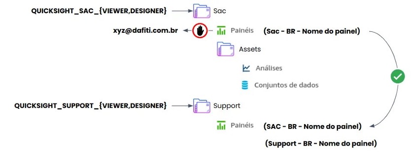
In this way, all users who join any of the groups will have exactly the same view as any of their peers, eliminating privileges in accessing data. In addition, the portfolio is enriched every day with reports that are created and maintained by other areas, but which may be of interest to areas other than the one responsible for creating it.
For this to work correctly, a certain rigidity is necessary in relation to the few naming and documentation standards that have been defined. On the other hand, designers have complete freedom to define the characteristics of their reports.
Another highlight in this model is that no report can be shared directly with a specific user; this restriction was defined using custom permissions in QuickSight. Therefore, the reports are always shared only through the folders. After all, we want the data to be accessible equally to everyone in the company.
Technical configurations
QuickSight offers a comprehensive API, and all the activities we carry out on a daily basis take place through these APIs. Among these activities, we highlight the granting of access and the monitoring of various aspects of the tool.
The QuickSight visual interface allows most of the tool’s maintenance activities to be performed and integration with Active Directory or the use of AWS Identity and Access Management (IAM) users is possible, but we understand that it wouldn’t be the ideal choice to grant access. Therefore, we defined an access grant flow for users and groups based on the QuickSight API, as can be seen in the following figure. In this model, the creation and removal of users is done through a JSON file with the following structure:
Whenever a user needs to be added or changed, the file is edited and a pull request is submitted to GitHub. If the request is approved, an action is triggered to send the file to an Amazon Simple Storage Service (Amazon S3) bucket. From this, an AWS Lambda function is triggered that performs two activities: the first is the maintenance of users and groups, and the second is the sending of an invitation through Amazon Simple Email Service (Amazon SES) for users to join QuickSight. In our case, we opted for a personalized invitation model that would emphasize the data democratization initiative that is being conducted.
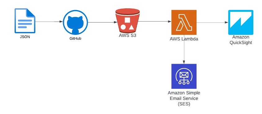
To monitor the tool, we implemented the architecture shown in the following figure, in which we used AWS CloudTrail to pull out the QuickSight logs and the QuickSight API to extract information from the tool’s resources, such as reports, users, datasets, data sources, and more. All of this data is processed by Glove, our data integration tool, stored in Amazon Redshift, and analyzed in QuickSight itself. This allows us to understand the behavior of our users and concentrate efforts on the most-used resources, in addition to allowing optimal cost control and the use of SPICE.
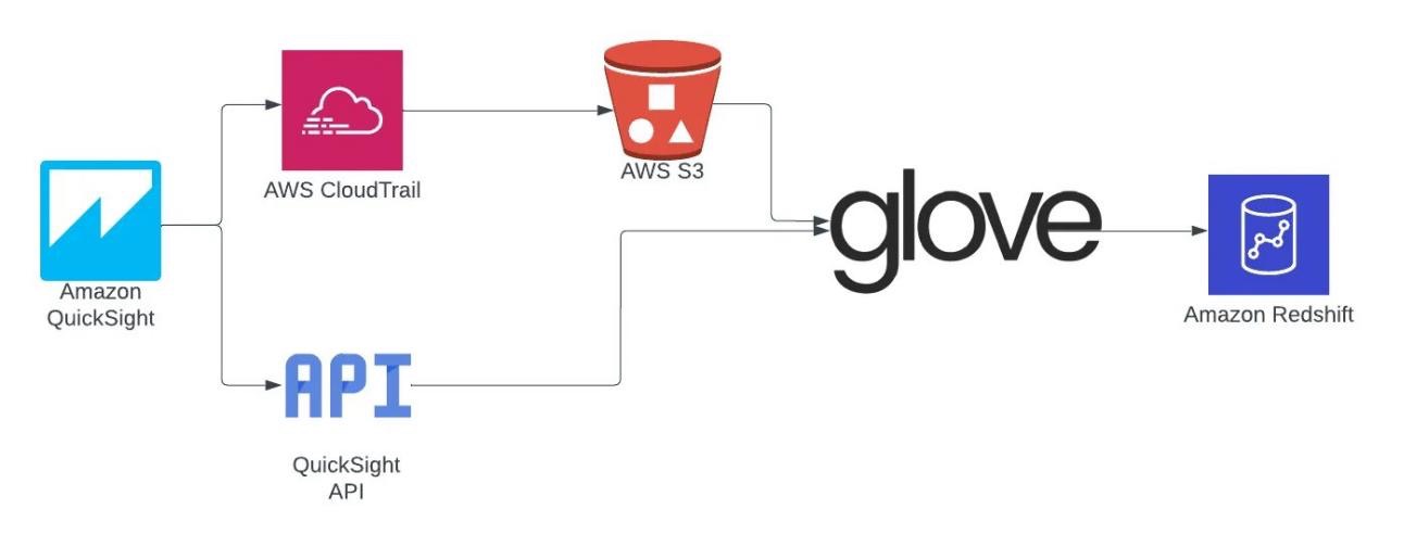
To update the datasets, we don’t use the QuickSight internal scheduler, due to the large volume of data and the complexity of the DAGs. We prefer updating the datasets within our ETL (extract, transform, and load) and ELT process orchestration flow. For this purpose, we use Hanger, our orchestration tool. This approach allows the datasets to be updated only when the data source is changed and the data quality processes are executed. This model is represented by the following figure.
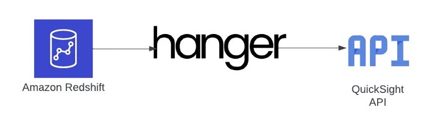
Conclusion
Choosing a data visualization tool is not a simple task. It involves many considerations, and several aspects must be analyzed in order for the choice to fit the characteristics of the company and to be consistent with the profile of business users.
For Dafiti, QuickSight was a natural choice from the moment we learned about its features. We needed a service that was in the same cloud as our main data sources, extremely fast using SPICE, and solved the maintenance and cost problem of on-premises applications. In terms of functionalities that are necessary for our business, it met our needs perfectly.
Do you want to know more about what we are doing in the data area here at Dafiti? Check out the following videos:
- AWS Summit SP 2022 – Dafiti, habilitando uma Empresa Data Driven na AWS
- Caso de sucesso: Dafiti reduz custos em 70% e otimiza tomadas de decisões com dados na nuvem da AWS
About the Authors
 Valdiney Gomes is Data Engineering Coordinator at Dafiti. He worked for many years in software engineering, migrated to data engineering, and currently leads an amazing team responsible for the data platform for Dafiti in Latin America.
 Hélio Leal is a Data Engineering Specialist at Dafiti, responsible for maintaining and evolving the entire data platform at Dafiti using AWS solutions.
 Flávia Lima is a Data Engineer at Dafiti, responsible for sustaining the data platform and providing the data from many sources to internal customers.
Implementing an effective data sharing strategy that satisfies compliance and regulatory requirements is complex. Customers often need to share data between disparate software as a service (SaaS) platforms within their organization or across organizations. On many occasions, they need to apply business logic to the data received from the source SaaS platform before pushing it to the target SaaS platform.
Let’s take an example. AnyCompany’s marketing team hosted an event at the Anaheim Convention Center, CA. The marketing team created leads based on the event in Adobe Marketo. An automated process downloaded the leads from Marketo in the marketing AWS account. These leads are then pushed to the sales AWS account. A business process picks up those leads, filters them based on a “Do Not Call” criteria, and creates entries in the Salesforce system. Now, the sales team can pursue those leads and continue to track the opportunities in Salesforce.
In this post, we show how to share your data across SaaS platforms in a cross-account structure using fully managed, low-code AWS services such as Amazon AppFlow, Amazon EventBridge, AWS Step Functions, and AWS Glue.
Solution overview
Considering our example of AnyCompany, let’s look at the data flow. AnyCompany’s Marketo instance is integrated with the producer AWS account. As the leads from Marketo land in the producer AWS account, they’re pushed to the consumer AWS account, which is integrated to Salesforce. Business logic is applied to the leads data in the consumer AWS account, and then the curated data is loaded into Salesforce.
We have used a serverless architecture to implement this use case. The following AWS services are used for data ingestion, processing, and load:
- Amazon AppFlow is a fully managed integration service that enables you to securely transfer data between SaaS applications like Salesforce, SAP, Marketo, Slack, and ServiceNow, and AWS services like Amazon S3 and Amazon Redshift, in just a few clicks. With AppFlow, you can run data flows at nearly any scale at the frequency you choose—on a schedule, in response to a business event, or on demand. You can configure data transformation capabilities like filtering and validation to generate rich, ready-to-use data as part of the flow itself, without additional steps. Amazon AppFlow is used to download leads data from Marketo and upload the curated leads data into Salesforce.
- Amazon EventBridge is a serverless event bus that lets you receive, filter, transform, route, and deliver events. EventBridge is used to track the events like receiving the leads data in the producer or consumer AWS accounts and then triggering a workflow.
- AWS Step Functions is a visual workflow service that helps developers use AWS services to build distributed applications, automate processes, orchestrate microservices, and create data and machine learning (ML) pipelines. Step Functions is used to orchestrate the data processing.
- AWS Glue is a serverless data preparation service that makes it easy to run extract, transform, and load (ETL) jobs. An AWS Glue job encapsulates a script that reads, processes, and then writes data to a new schema. This solution uses Python 3.6 AWS Glue jobs for data filtration and processing.
- Amazon Simple Storage Service (Amazon S3) is an object storage service offering industry-leading scalability, data availability, security, and performance. Amazon S3 is used to store the leads data.
Let’s review the architecture in detail. The following diagram shows a visual representation of how this integration works.

The following steps outline the process for transferring and processing leads data using Amazon AppFlow, Amazon S3, EventBridge, Step Functions, AWS Glue, and Salesforce:
- Amazon AppFlow runs on a daily schedule and retrieves any new leads created within the last 24 hours (incremental changes) from Marketo.
- The leads are saved as Parquet format files in an S3 bucket in the producer account.
- When the daily flow is complete, Amazon AppFlow emits events to EventBridge.
- EventBridge triggers Step Functions.
- Step Functions copies the Parquet format files containing the leads from the producer account’s S3 bucket to the consumer account’s S3 bucket.
- Upon a successful file transfer, Step Functions publishes an event in the consumer account’s EventBridge.
- An EventBridge rule intercepts this event and triggers Step Functions in the consumer account.
- Step Functions calls an AWS Glue crawler, which scans the leads Parquet files and creates a table in the AWS Glue Data Catalog.
- The AWS Glue job is called, which selects records with the Do Not Call field set to false from the leads files, and creates a new set of curated Parquet files. We have used an AWS Glue job for the ETL pipeline to showcase how you can use purpose-built analytics service for complex ETL needs. However, for simple filtering requirements like Do Not Call, you can use the existing filtering feature of Amazon AppFlow.
- Step Functions then calls Amazon AppFlow.
- Finally, Amazon AppFlow populates the Salesforce leads based on the data in the curated Parquet files.
We have provided artifacts in this post to deploy the AWS services in your account and try out the solution.
Prerequisites
To follow the deployment walkthrough, you need two AWS accounts, one for the producer and other for the consumer. Use us-east-1 or us-west-2 as your AWS Region.
Consumer account setup:
Stage the data
To prepare the data, complete the following steps:
- Download the zipped archive file to use for this solution and unzip the files locally.
The AWS Glue job uses the glue-job.py script to perform ETL and populates the curated table in the Data Catalog.
- Create an S3 bucket called
consumer-configbucket-<ACCOUNT\_ID>via the Amazon S3 console in the consumer account, whereACCOUNT\_IDis your AWS account ID. - Upload the script to this location.
Create a connection to Salesforce
Follow the connection setup steps outlined in here. Please make a note of the Salesforce connector name.
Create a connection to Salesforce in the consumer account
Follow the connection setup steps outlined in Create Opportunity Object Flow.
Set up resources with AWS CloudFormation
We provided two AWS CloudFormation templates to create resources: one for the producer account, and one for the consumer account.
Amazon S3 now applies server-side encryption with Amazon S3 managed keys (SSE-S3) as the base level of encryption for every bucket in Amazon S3. Starting January 5, 2023, all new object uploads to Amazon S3 are automatically encrypted at no additional cost and with no impact on performance. We use this default encryption for both producer and consumer S3 buckets. If you choose to bring your own keys with AWS Key Management Service (AWS KMS), we recommend referring to Replicating objects created with server-side encryption (SSE-C, SSE-S3, SSE-KMS) for cross-account replication.
Launch the CloudFormation stack in the consumer account
Let’s start with creating resources in the consumer account. There are a few dependencies on the consumer account resources from the producer account. To launch the CloudFormation stack in the consumer account, complete the following steps:
- Sign in to the consumer account’s AWS CloudFormation console in the target Region.
- Choose Launch Stack.
- Choose Next.
- For Stack name, enter a stack name, such as
stack-appflow-consumer. - Enter the parameters for the connector name, object, and producer (source) account ID.
- Choose Next.

- On the next page, choose Next.
- Review the details on the final page and select I acknowledge that AWS CloudFormation might create IAM resources.
- Choose Create stack.
Stack creation takes approximately 5 minutes to complete. It will create the following resources. You can find them on the Outputs tab of the CloudFormation stack.
- ConsumerS3Bucket –
consumer-databucket-<consumer account id> - Consumer S3 Target Folder –
marketo-leads-source - ConsumerEventBusArn –
arn:aws:events:<region>:<consumer account id>:event-bus/consumer-custom-event-bus - ConsumerEventRuleArn –
arn:aws:events:<region>:<consumer account id>:rule/consumer-custom-event-bus/consumer-custom-event-bus-rule - ConsumerStepFunction –
arn:aws:states:<region>:<consumer account id>:stateMachine:consumer-state-machine - ConsumerGlueCrawler –
consumer-glue-crawler - ConsumerGlueJob –
consumer-glue-job - ConsumerGlueDatabase –
consumer-glue-database - ConsumerAppFlow –
arn:aws:appflow:<region>:<consumer account id>:flow/consumer-appflow
Producer account setup:
Create a connection to Marketo
Follow the connection setup steps outlined in here. Please make a note of the Marketo connector name.
Launch the CloudFormation stack in the producer account
Now let’s create resources in the producer account. Complete the following steps:
- Sign in to the producer account’s AWS CloudFormation console in the source Region.
- Choose Launch Stack.
- Choose Next.
- For Stack name, enter a stack name, such as
stack-appflow-producer. - Enter the following parameters and leave the rest as default:
- AppFlowMarketoConnectorName: name of the Marketo connector, created above
- ConsumerAccountBucket:
consumer-databucket-<consumer account id> - ConsumerAccountBucketTargetFolder:
marketo-leads-source - ConsumerAccountEventBusArn:
arn:aws:events:<region>:<consumer account id>:event-bus/consumer-custom-event-bus - DefaultEventBusArn:
arn:aws:events:<region>:<producer account id>:event-bus/default


- Choose Next.
- On the next page, choose Next.
- Review the details on the final page and select I acknowledge that AWS CloudFormation might create IAM resources.
- Choose Create stack.
Stack creation takes approximately 5 minutes to complete. It will create the following resources. You can find them on the Outputs tab of the CloudFormation stack.
- Producer AppFlow –
producer-flow - Producer Bucket –
arn:aws:s3:::producer-bucket.<region>.<producer account id> - Producer Flow Completion Rule –
arn:aws:events:<region>:<producer account id>:rule/producer-appflow-completion-event - Producer Step Function –
arn:aws:states:<region>:<producer account id>:stateMachine:ProducerStateMachine-xxxx - Producer Step Function Role –
arn:aws:iam::<producer account id>:role/service-role/producer-stepfunction-role
- After successful creation of the resources, go to the consumer account S3 bucket,
consumer-databucket-<consumer account id>, and update the bucket policy as follows:
Validate the workflow
Let’s walk through the flow:
- Review the Marketo and Salesforce connection setup in the producer and consumer account respectively.
In the architecture section, we suggested scheduling the AppFlow (producer-flow) in the producer account. However, for quick testing purposes, we demonstrate how to manually run the flow on demand.
- Go to the AppFlow (
producer-flow) in the producer account. On the Filters tab of the flow, choose Edit filters. - Choose the Created At date range for which you have data.

- Save the range and choose Run flow.

- Review the producer S3 bucket.
AppFlow generates the files in the producer-flow prefix within this bucket. The files are temporarily located in the producer S3 bucket under s3://<producer-bucket>.<region>.<account-id>/producer-flow.
- Review the EventBridge rule and Step Functions state machine in the producer account.
The Amazon AppFlow job completion triggers an EventBridge rule (arn:aws:events:<region>:<producer account id>:rule/producer-appflow-completion-event, as noted in the Outputs tab of the CloudFromation stack in the Producer Account), which triggers the Step Functions state machine (arn:aws:states:<region>:<producer account id>:stateMachine:ProducerStateMachine-xxxx) in the producer account. The state machine copies the files to the consumer S3 bucket from the producer-flow prefix in the producer S3 bucket. Once file copy is complete, the state machine moves the files from the producer-flow prefix to the archive prefix in the producer S3 bucket. You can find the files in s3://<producer-bucket>.<region>.<account-id>/archive.


- Review the consumer S3 bucket.
The Step Functions state machine in the producer account copies the files to the consumer S3 bucket and sends an event to EventBridge in the consumer account. The files are located in the consumer S3 bucket under s3://consumer-databucket-<account-id>/marketo-leads-source/.
- Review the EventBridge rule (
arn:aws:events:<region>:<consumer account id>:rule/consumer-custom-event-bus/consumer-custom-event-bus-rule) in the consumer account, which should have triggered the Step Function workflow (arn:aws:states:<region>:<consumer account id>:stateMachine:consumer-state-machine).
The AWS Glue crawler (consumer-glue-crawler) runs to update the metadata followed by the AWS Glue job (consumer-glue-job), which curates the data by applying the Do not call filter. The curated files are placed in s3://consumer-databucket-<account-id>/marketo-leads-curated/. After data curation, the flow is started as part of the state machine.

- Review the Amazon AppFlow job (
arn:aws:appflow:<region>:<consumer account id>:flow/consumer-appflow) run status in the consumer account.
Upon a successful run of the Amazon AppFlow job, the curated data files are moved to the s3://consumer-databucket-<account-id>/marketo-leads-processed/ folder and Salesforce is updated with the leads. Additionally, all the original source files are moved from s3://consumer-databucket-<account-id>/marketo-leads-source/ to s3://consumer-databucket-<account-id>/marketo-leads-archive/.
- Review the updated data in Salesforce.
You will see newly created or updated leads created by Amazon AppFlow.

Clean up
To clean up the resources created as part of this post, delete the following resources:
- Delete the resources in the producer account:
- Delete the producer S3 bucket content.
- Delete the CloudFormation stack.
- Delete the resources in the consumer account:
- Delete the consumer S3 bucket content.
- Delete the CloudFormation stack.
Summary
In this post, we showed how you can support a cross-account model to exchange data between different partners with different SaaS integrations using Amazon AppFlow. You can expand this idea to support multiple target accounts.
For more information, refer to Simplifying cross-account access with Amazon EventBridge resource policies. To learn more about Amazon AppFlow, visit Amazon AppFlow.
About the authors
 Ramakant Joshi is an AWS Solutions Architect, specializing in the analytics and serverless domain. He has a background in software development and hybrid architectures, and is passionate about helping customers modernize their cloud architecture.
 Debaprasun Chakraborty is an AWS Solutions Architect, specializing in the analytics domain. He has around 20 years of software development and architecture experience. He is passionate about helping customers in cloud adoption, migration and strategy.
 Suraj Subramani Vineet is a Senior Cloud Architect at Amazon Web Services (AWS) Professional Services in Sydney, Australia. He specializes in designing and building scalable and cost-effective data platforms and AI/ML solutions in the cloud. Outside of work, he enjoys playing soccer on weekends.
AWS has been named a Challenger in the 2023 Gartner Magic Quadrant for Analytics and Business Intelligence (ABI) Platforms. Previously, AWS was positioned as a Niche player in the Magic Quadrant for ABI platforms. The Gartner Magic Quadrant evaluates 20 ABI companies based on their Ability to Execute and Completeness of Vision.
In our view, this recognition in the Magic Quadrant reinforces the progress we have made by tirelessly innovating on behalf of our customers. And this is just the beginning.
Benefits of QuickSight
AWS built QuickSight from the ground up as a cloud BI service to overcome challenges customers faced with alternative offerings. QuickSight powers data-driven organizations with unified business intelligence at hyperscale. With QuickSight, organizations of any size can meet the analytical needs of all users from the same source of truth through modern interactive dashboards, paginated reports, embedded analytics, and natural language queries. Since introducing QuickSight in 2016, we have been on a journey to democratize access to data for everyone in an organization. In 2022 alone, QuickSight added more than 80 capabilities, making it easier for you to deliver valuable business insights throughout your organization, when and where needed.
Today, over 100,000 customers use QuickSight as their BI service. Organizations of all sizes are choosing QuickSight for their BI needs and enabling users to understand, visualize, and derive insights and predictions from data, regardless of technical expertise.
Review the Gartner Magic Quadrant

Access a complimentary copy of the full report to see why Gartner positioned AWS as a Challenger, and dive deep into the strengths and cautions of AWS.
We are excited about our momentum, strong vision, and the pace at which we are enabling our customers to democratize access to data for everyone in their organization.
Gartner Disclaimer
Gartner does not endorse any vendor, product or service depicted in its research publications, and does not advise technology users to select only those vendors with the highest ratings. Gartner research publications consist of the opinions of Gartner’s research organization and should not be construed as statements of fact. Gartner disclaims all warranties, expressed or implied, with respect to this research, including any warranties of merchantability or fitness for a particular purpose.
Gartner, Magic Quadrant for Analytics and Business Intelligence Platforms, Kurt Schlegel, Julian Sun, David Pidsley, Anirudh Ganeshan, Fay Fei, Aura Popa, Radu Miclaus, Edgar Macari, Kevin Quinn, Christopher Long, 5 April 2023
Gartner is a registered trademark and service mark and Magic Quadrant is a registered trademark of Gartner, Inc. and/or its affiliates in the U.S. and internationally and are used herein with permission. All rights reserved
This graphic was published by Gartner, Inc. as part of a larger research document and should be evaluated in the context of the entire document. The Gartner document is available upon request from Amazon Web Services, Inc.
About the Author
 Jose Kunnackal is Director of Product Management for Amazon QuickSight, AWS’ cloud-native, fully managed BI service. Jose started his career with Motorola, writing software for telecom and first responder systems. Later he was Director of Engineering at Trilibis Mobile, where he built a SaaS mobile web platform using AWS services. Jose is excited by the potential of cloud technologies to help customers make the most of their data.
Building a data lake on Amazon Simple Storage Service (Amazon S3) provides numerous benefits for an organization. It allows you to access diverse data sources, build business intelligence dashboards, build AI and machine learning (ML) models to provide customized customer experiences, and accelerate the curation of new datasets for consumption by adopting a modern data architecture or data mesh architecture.
However, many use cases, like performing change data capture (CDC) from an upstream relational database to an Amazon S3-based data lake, require handling data at a record level. Performing an operation like inserting, updating, and deleting individual records from a dataset requires the processing engine to read all the objects (files), make the changes, and rewrite entire datasets as new files. Furthermore, making the data available in the data lake in near-real time often leads to the data being fragmented over many small files, resulting in poor query performance and compaction maintenance.
In 2022, we announced that you can enforce fine-grained access control policies using AWS Lake Formation and query data stored in any supported file format using table formats such as Apache Iceberg, Apache Hudi, and more using Amazon Athena queries. You get the flexibility to choose the table and file format best suited for your use case and get the benefit of centralized data governance to secure data access when using Athena.
In this post, we show you how to configure Lake Formation using Iceberg table formats. We also explain how to upsert and merge in an S3 data lake using an Iceberg framework and apply Lake Formation access control using Athena.
Iceberg is an open table format for very large analytic datasets. Iceberg manages large collections of files as tables, and it supports modern analytical data lake operations such as record-level insert, update, delete, and time travel queries. The Iceberg specification allows seamless table evolution such as schema and partition evolution, and its design is optimized for usage on Amazon S3. Iceberg also helps guarantee data correctness under concurrent write scenarios.
Solution overview
To explain this setup, we present the following architecture, which integrates Amazon S3 for the data lake (Iceberg table format), Lake Formation for access control, AWS Glue for ETL (extract, transform, and load), and Athena for querying the latest inventory data from the Iceberg tables using standard SQL.
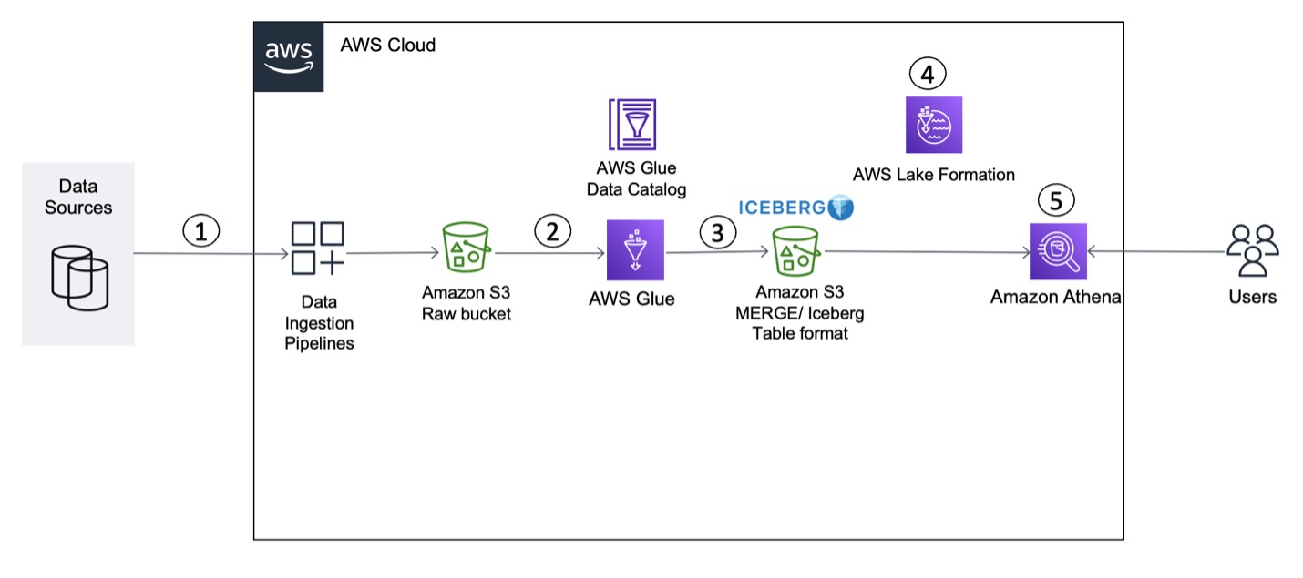
The solution workflow consists of the following steps, including data ingestion (Steps 1–3), data governance (Step 4), and data access (Step 5):
- We use AWS Database Migration Service (AWS DMS) or a similar tool to connect to the data source and move incremental data (CDC) to Amazon S3 in CSV format.
- An AWS Glue PySpark job reads the incremental data from the S3 input bucket and performs deduplication of the records.
- The job then invokes Iceberg’s MERGE statements to merge the data with the target S3 bucket.
- We use the AWS Glue Data Catalog as a centralized catalog, which is used by AWS Glue and Athena. An AWS Glue crawler is integrated on top of S3 buckets to automatically detect the schema. Lake Formation allows you to centrally manage permissions and access control for Data Catalog resources in your S3 data lake. You can use fine-grained access control in Lake Formation to restrict access to data in query results.
- We use Athena integrated with Lake Formation to query data from the Iceberg table using standard SQL and validate table- and column-level access on Iceberg tables.
For this solution, we assume that the raw data files are already available in Amazon S3, and focus on processing the data using AWS Glue with Iceberg table format. We use sample item data that has the following attributes:
- op – This represents the operation on the source record. This shows values I to represent insert operations, U to represent updates, and D to represent deletes. You need to make sure this attribute is included in your CDC incremental data before it gets written to Amazon S3. Make sure you capture this attribute, so that your ETL logic can take appropriate action while merging it.
- product\_id – This is the primary key column in the source data table.
- category – This column represents the category of an item.
- product\_name – This is the name of the product.
- quantity\_available – This is the quantity available in the inventory. When we showcase the incremental data for UPSERT or MERGE, we reduce the quantity available for the product to showcase the functionality.
- last\_update\_time – This is the time when the item record was updated at the source data.
We demonstrate implementing the solution with the following steps:
- Create an S3 bucket for input and output data.
- Create input and output tables using Athena.
- Insert the data into the Iceberg table from Athena.
- Query the Iceberg table using Athena.
- Upload incremental (CDC) data for further processing.
- Run the AWS Glue job again to process the incremental files.
- Query the Iceberg table again using Athena.
- Define Lake Formation policies.
Prerequisites
For Athena queries, we need to configure an Athena workgroup with engine version 3 to support Iceberg table format.

To validate cross-account access through Lake Formation for Iceberg table, in this post we used two accounts (primary and secondary).
Now let’s dive into the implementation steps.
Create an S3 bucket for input and output data
Before we run the AWS Glue job, we have to upload the sample CSV files to the input bucket and process them with AWS Glue PySpark code for the output.
To create an S3 bucket, complete the following steps:
- On the Amazon S3 console, choose Buckets in the navigation pane.
- Choose Create bucket.
- Specify the bucket name as
iceberg-blogand leave the remaining fields as default.
S3 bucket names are globally unique. While implementing the solution, you may get an error saying the bucket name already exists. Make sure to provide a unique name and use the same name while implementing the rest of the implementation steps. Formatting the bucket name as<Bucket-Name>-${AWS\_ACCOUNT\_ID}-${AWS\_REGION\_CODE}might help you get a unique name.
- On the bucket details page, choose Create folder.
- Create two subfolders. For this post, we create
iceberg-blog/raw-csv-inputandiceberg-blog/iceberg-output.

- Upload the
LOAD00000001.csvfile into theraw-csv-inputfolder.
The following screenshot provides a sample of the input dataset.

Create input and output tables using Athena
To create input and output Iceberg tables in the AWS Glue Data Catalog, open the Athena query editor and run the following queries in sequence:
As we explain later in this post, it’s essential to record the data locations when incorporating Lake Formation access controls.
Alternatively, you can use an AWS Glue crawler to create the table definition for the input files.
Insert the data into the Iceberg table from Athena
Optionally, we can insert data into the Iceberg table through Athena using the following code:
For this post, we load the data using an AWS Glue job. Complete the following steps to create the job:
- On the AWS Glue console, choose Jobs in the navigation pane.
- Choose Create job.
- Select Visual with a blank canvas.
- Choose Create.

- Choose Edit script.

- Replace the script with the following script:
- On the Job details tab, specify the job name (
iceberg-lf). - For IAM Role, assign an AWS Identity and Access Management (IAM) role that has the required permissions to run an AWS Glue job and read and write to the S3 bucket.
- For Glue version, choose Glue 4.0 (Glue 3.0 is also supported).
- For Language, choose Python 3.
- Make sure Job bookmark has the default value of Enable.

- For Job parameters, add the following:
- Add the key
--datalake-formatswith the valueiceberg. - Add the key
--iceberg\_job\_catalog\_warehousewith the value as your S3 path (s3://<bucket-name>/<iceberg-warehouse-path>).

- Add the key
- Choose Save and then Run, which should write the input data to the Iceberg table with a MERGE statement.
Query the Iceberg table using Athena
After you have successfully run the AWS Glue job, you can validate the output in Athena with the following SQL query:
The output of the query should match the input, with one difference: the Iceberg output table doesn’t have theopcolumn.

Upload incremental (CDC) data for further processing
After we process the initial full load file, let’s upload an incremental file.

This file includes updated records on two items.

Run the AWS Glue job again to process incremental files
Because the AWS Glue job has bookmarks enabled, the job picks up the new incremental file and performs a MERGE operation on the Iceberg table.
To run the job again, complete the following steps:
- On the AWS Glue console, choose Jobs in the navigation pane.
- Select the job and choose Run.
For this post, we run the job manually, but you can configure your AWS Glue jobs to run as part of an AWS Glue workflow or via AWS Step Functions (for more information, see Manage AWS Glue Jobs with Step Functions).
Query the Iceberg table using Athena after incremental data processing
When the incremental data processing is complete, you can run the same SELECT statement again and validate that the quantity value is updated for items 200 and 201.
The following screenshot shows the output.

Define Lake Formation policies
For data governance, we use Lake Formation. Lake Formation is a fully managed service that simplifies data lake setup, supports centralized security management, and provides transactional access on top of your data lake. Moreover, it enables data sharing across accounts and organizations. There are two ways to share data resources in Lake Formation: named resource access control (NRAC) and tag-based access control (TBAC). NRAC uses AWS Resource Access Manager (AWS RAM) to share data resources across accounts using Lake Formation V3. Those are consumed via resource links that are based on created resource shares. Lake Formation tag-based access control (LF-TBAC) is another approach to share data resources in Lake Formation, which defines permissions based on attributes. These attributes are called LF-tags.
In this example, we create databases in the primary account. Our NRAC database is shared with a data domain via AWS RAM. Access to data tables that we register in this database will be handled through NRAC.
Configure access controls in the primary account
In the primary account, complete the following steps to set up access controls using Lake Formation:
- On the Lake Formation console, choose Data lake locations in the navigation pane.
- Choose Register location.
- Update the Iceberg Amazon S3 location path shown in the following screenshot.

Grant access to the database to the secondary account
To grant database access to the external (secondary) account, complete the following steps:
- On the Lake Formation console, navigate to your database.
- On the Actions menu, choose Grant.

- Choose External accounts and enter the secondary account number.
- Select Named data catalog resources.
- Verify the database name.
The first grant should be at database level, and the second grant is at table level.
- For Database permissions, specify your permissions (for this post, we select Describe).
- Choose Grant.

Now you need to grant permissions at the table level.
- Select External accounts and enter the secondary account number.
- Select Named data catalog resources.
- Verify the table name.
- For Table permissions, specify the permissions you want to grant. For this post, we select Select and Describe.
- Choose Grant.

If you see the following error, you must revokeIAMAllowedPrincipalsfrom the data lake permissions.

To do so, select IAMAllowedPrincipals and choose Revoke.

Choose Revoke again to confirm.

After you revoke the data permissions, the permissions should appear as shown in the following screenshot.

Add AWS Glue IAM role permissions
Because the IAM principal role was revoked, the AWS Glue IAM role that was used in the AWS Glue job needs to be added exclusively to grant access as shown in the following screenshot.

You need to repeat these steps for the AWS Glue IAM role at table level.

Verify the permissions granted to the AWS Glue IAM role on the Lake Formation console.

Grant access to the Iceberg table to the external account
In the secondary account, complete the following steps to grant access to the Iceberg table to external account.
- On the AWS RAM console, choose Resource shares in the navigation pane.
- Choose the resource shares invitation sent from the primary account.

- Choose Accept resource share.

The resource status should now be active.

Next, you need to create a resource link for the shared Iceberg table and access through Athena.
- On the Lake Formation console, choose Tables in the navigation pane.
- Select the Iceberg table (shared from the primary account).
- On the Actions menu, choose Create resource link.

- For Resource link name, enter a name (for this post,
iceberg\_table\_lf\_demo). - For Database, choose your database and verify the shared table and database are automatically populated.
- Choose Create.

- Select your table and on the Actions menu, choose View data.

You’re redirected to the Athena console, where you can query the data.

Grant column-based access in the primary account
For column-level restricted access, you need to grant access at the column level on the Iceberg table. Complete the following steps:
- On the Lake Formation console, navigate to your database.
- On the Actions menu, choose Grant.
- Select External accounts and enter the secondary account number.
- Select Named data catalog resources.
- Verify the table name.
- For Table permissions, choose the permissions you want to grant. For this post, we select Select.
- Under Data permissions, choose Column-based access.
- Select Include columns and choose your permission filters (for this post,
CategoryandQuantity\_available). - Choose Grant.

Data with restricted columns can now be queried through the Athena console.

Clean up
To avoid incurring ongoing costs, complete the following steps to clean up your resources:
- In your secondary account, log in to the Lake Formation console.
- Drop the resource share table.
- In your primary account, log in to the Lake Formation console.
- Revoke the access you configured.
- Drop the AWS Glue tables and database.
- Delete the AWS Glue job.
- Delete the S3 buckets and any other resources that you created as part of the prerequisites for this post.
Conclusion
This post explains how you can use the Iceberg framework with AWS Glue and Lake Formation to define cross-account access controls and query data using Athena. It provides an overview of Iceberg and its features and integration approaches, and explains how you can ingest data, grant cross-account access, and query data through a step-by-step guide.
We hope this gives you a great starting point for using Iceberg to build your data lake platform along with AWS analytics services to implement your solution.
About the Authors
 Vikram Sahadevan is a Senior Resident Architect on the AWS Data Lab team. He enjoys efforts that focus around providing prescriptive architectural guidance, sharing best practices, and removing technical roadblocks with joint engineering engagements between customers and AWS technical resources that accelerate data, analytics, artificial intelligence, and machine learning initiatives.
 Suvendu Kumar Patra possesses 18 years of experience in infrastructure, database design, and data engineering, and he currently holds the position of Senior Resident Architect at Amazon Web Services. He is a member of the specialized focus group, AWS Data Lab, and his primary duties entail working with executive leadership teams of strategic AWS customers to develop their roadmaps for data, analytics, and AI/ML. Suvendu collaborates closely with customers to implement data engineering, data hub, data lake, data governance, and EDW solutions, as well as enterprise data strategy and data management.
Customers use Amazon Redshift to run their business-critical analytics on petabytes of structured and semi-structured data. Apache Spark is a popular framework that you can use to build applications for use cases such as ETL (extract, transform, and load), interactive analytics, and machine learning (ML). Apache Spark enables you to build applications in a variety of languages, such as Java, Scala, and Python, by accessing the data in your Amazon Redshift data warehouse.
Amazon Redshift integration for Apache Spark helps developers seamlessly build and run Apache Spark applications on Amazon Redshift data. Developers can use AWS analytics and ML services such as Amazon EMR, AWS Glue, and Amazon SageMaker to effortlessly build Apache Spark applications that read from and write to their Amazon Redshift data warehouse. You can do so without compromising on the performance of your applications or transactional consistency of your data.
In this post, we discuss why Amazon Redshift integration for Apache Spark is critical and efficient for analytics and ML. In addition, we discuss use cases that use Amazon Redshift integration with Apache Spark to drive business impact. Finally, we walk you through step-by-step examples of how to use this official AWS connector in an Apache Spark application.
Amazon Redshift integration for Apache Spark
The Amazon Redshift integration for Apache Spark minimizes the cumbersome and often manual process of setting up a spark-redshift connector (community version) and shortens the time needed to prepare for analytics and ML tasks. You only need to specify the connection to your data warehouse, and you can start working with Amazon Redshift data from your Apache Spark-based applications within minutes.
You can use several pushdown capabilities for operations such as sort, aggregate, limit, join, and scalar functions so that only the relevant data is moved from your Amazon Redshift data warehouse to the consuming Apache Spark application. This allows you to improve the performance of your applications. Amazon Redshift admins can easily identify the SQL generated from Spark-based applications. In this post, we show how you can find out the SQL generated by the Apache Spark job.
Moreover, Amazon Redshift integration for Apache Spark uses Parquet file format when staging the data in a temporary directory. Amazon Redshift uses the UNLOAD SQL statement to store this temporary data on Amazon Simple Storage Service (Amazon S3). The Apache Spark application retrieves the results from the temporary directory (stored in Parquet file format), which improves performance.
You can also help make your applications more secure by utilizing AWS Identity and Access Management (IAM) credentials to connect to Amazon Redshift.
Amazon Redshift integration for Apache Spark is built on top of the spark-redshift connector (community version) and enhances it for performance and security, helping you gain up to 10 times faster application performance.
Use cases for Amazon Redshift integration with Apache Spark
For our use case, the leadership of the product-based company wants to know the sales for each product across multiple markets. As sales for the company fluctuate dynamically, it has become a challenge for the leadership to track the sales across multiple markets. However, the overall sales are declining, and the company leadership wants to find out which markets aren’t performing so that they can target these markets for promotion campaigns.
For sales across multiple markets, the product sales data such as orders, transactions, and shipment data is available on Amazon S3 in the data lake. The data engineering team can use Apache Spark with Amazon EMR or AWS Glue to analyze this data in Amazon S3.
The inventory data is available in Amazon Redshift. Similarly, the data engineering team can analyze this data with Apache Spark using Amazon EMR or an AWS Glue job by using the Amazon Redshift integration for Apache Spark to perform aggregations and transformations. The aggregated and transformed dataset can be stored back into Amazon Redshift using the Amazon Redshift integration for Apache Spark.
Using a distributed framework like Apache Spark with the Amazon Redshift integration for Apache Spark can provide the visibility across the data lake and data warehouse to generate sales insights. These insights can be made available to the business stakeholders and line of business users in Amazon Redshift to make informed decisions to run targeted promotions for the low revenue market segments.
Additionally, we can use the Amazon Redshift integration with Apache Spark in the following use cases:
- An Amazon EMR or AWS Glue customer running Apache Spark jobs wants to transform data and write that into Amazon Redshift as a part of their ETL pipeline
- An ML customer uses Apache Spark with SageMaker for feature engineering for accessing and transforming data in Amazon Redshift
- An Amazon EMR, AWS Glue, or SageMaker customer uses Apache Spark for interactive data analysis with data on Amazon Redshift from notebooks
Examples for Amazon Redshift integration for Apache Spark in an Apache Spark application
In this post, we show the steps to connect Amazon Redshift from Amazon EMR on Amazon Elastic Compute Cloud (Amazon EC2), Amazon EMR Serverless, and AWS Glue using a common script. In the following sample code, we generate a report showing the quarterly sales for the year 2008. To do that, we join two Amazon Redshift tables using an Apache Spark DataFrame, run a predicate pushdown, aggregate and sort the data, and write the transformed data back to Amazon Redshift. The script uses PySpark
The script uses IAM-based authentication for Amazon Redshift. IAM roles used by Amazon EMR and AWS Glue should have the appropriate permissions to authenticate Amazon Redshift, and access to an S3 bucket for temporary data storage.
The following example policy allows the IAM role to call the GetClusterCredentials operations:
The following example policy allows access to an S3 bucket for temporary data storage:
The complete script is as follows:
If you plan to use the preceding script in your environment, make sure you replace the values for the following variables with the appropriate values for your environment: jdbc\_iam\_url, temp\_dir, and aws\_role.
In the next section, we walk through the steps to run this script to aggregate a sample dataset that is made available in Amazon Redshift.
Prerequisites
Before we begin, make sure the following prerequisites are met:
- You have an AWS account
- You have access to create AWS CloudFormation stack
Deploy resources using AWS CloudFormation
Complete the following steps to deploy the CloudFormation stack:
- Sign in to the AWS Management Console, then launch the CloudFormation stack:
You can also download the CloudFormation template to create the resources mentioned in this post through infrastructure as code (IaC). Use this template when launching a new CloudFormation stack.
- Scroll down to the bottom of the page to select I acknowledge that AWS CloudFormation might create IAM resources under Capabilities, then choose Create stack.

The stack creation process takes 15–20 minutes to complete. The CloudFormation template creates the following resources:
-
- An Amazon VPC with the needed subnets, route tables, and NAT gateway
- An S3 bucket with the name
redshift-spark-databucket-xxxxxxx(note that xxxxxxx is a random string to make the bucket name unique) - An Amazon Redshift cluster with sample data loaded inside the database
devand the primary userredshiftmasteruser. For the purpose of this blog post,redshiftmasteruserwith administrative permissions is used. However, it is recommended to use a user with fine grained access control in production environment. - An IAM role to be used for Amazon Redshift with the ability to request temporary credentials from the Amazon Redshift cluster’s dev database
- Amazon EMR Studio with the needed IAM roles
- Amazon EMR release version 6.9.0 on an EC2 cluster with the needed IAM roles
- An Amazon EMR Serverless application release version 6.9.0
- An AWS Glue connection and AWS Glue job version 4.0
- A Jupyter notebook to run using Amazon EMR Studio using Amazon EMR on an EC2 cluster
- A PySpark script to run using Amazon EMR Studio and Amazon EMR Serverless
- After the stack creation is complete, choose the stack name
redshift-sparkand navigate to the Outputs
We utilize these output values later in this post.

In the next sections, we show the steps for Amazon Redshift integration for Apache Spark from Amazon EMR on Amazon EC2, Amazon EMR Serverless, and AWS Glue.
Use Amazon Redshift integration with Apache Spark on Amazon EMR on EC2
Starting from Amazon EMR release version 6.9.0 and above, the connector using Amazon Redshift integration for Apache Spark and Amazon Redshift JDBC driver are available locally on Amazon EMR. These files are located under the /usr/share/aws/redshift/ directory. However, in the previous versions of Amazon EMR, the community version of the spark-redshift connector is available.
The following example shows how to connect Amazon Redshift using a PySpark kernel via an Amazon EMR Studio notebook. The CloudFormation stack created Amazon EMR Studio, Amazon EMR on an EC2 cluster, and a Jupyter notebook available to run. To go through this example, complete the following steps:
- Download the Jupyter notebook made available in the S3 bucket for you:
- In the CloudFormation stack outputs, look for the value for
EMRStudioNotebook, which should point to theredshift-spark-emr.ipynbnotebook available in the S3 bucket. - Choose the link or open the link in a new tab by copying the URL for the notebook.
- After you open the link, download the notebook by choosing Download, which will save the file locally on your computer.

- In the CloudFormation stack outputs, look for the value for
- Access Amazon EMR Studio by choosing or copying the link provided in the CloudFormation stack outputs for the key
EMRStudioURL. - In the navigation pane, choose Workspaces.

- Choose Create Workspace.

- Provide a name for the Workspace, for instance
redshift-spark. - Expand the Advanced configuration section and select Attach Workspace to an EMR cluster.
- Under Attach to an EMR cluster, choose the EMR cluster with the name
emrCluster-Redshift-Spark. - Choose Create Workspace.

- After the Amazon EMR Studio Workspace is created and in Attached status, you can access the Workspace by choosing the name of the Workspace.
This should open the Workspace in a new tab. Note that if you have a pop-up blocker, you may have to allow the Workspace to open or disable the pop-up blocker.

In the Amazon EMR Studio Workspace, we now upload the Jupyter notebook we downloaded earlier.
- Choose Upload to browse your local file system and upload the Jupyter notebook (
redshift-spark-emr.ipynb).

- Choose (double-click) the
redshift-spark-emr.ipynbnotebook within the Workspace to open the notebook.

The notebook provides the details of different tasks that it performs. Note that in the section Define the variables to connect to Amazon Redshift cluster, you don’t need to update the values for jdbc\_iam\_url, temp\_dir, and aws\_role because these are updated for you by AWS CloudFormation. AWS CloudFormation has also performed the steps mentioned in the Prerequisites section of the notebook.
You can now start running the notebook.
- Run the individual cells by selecting them and then choosing Play.
You can also use the key combination of Shift+Enter or Shift+Return. Alternatively, you can run all the cells by choosing Run All Cells on the Run menu.
- Find the predicate pushdown operation performed on the Amazon Redshift cluster by the Amazon Redshift integration for Apache Spark.
We can also see the temporary data stored on Amazon S3 in the optimized Parquet format. The output can be seen from running the cell in the section Get the last query executed on Amazon Redshift.

- To validate the table created by the job from Amazon EMR on Amazon EC2, navigate to the Amazon Redshift console and choose the cluster
redshift-spark-redshift-clusteron the Provisioned clusters dashboard page.

- In the cluster details, on the Query data menu, choose Query in query editor v2.

- Choose the cluster in the navigation pane and connect to the Amazon Redshift cluster when it requests for authentication.
- Select Temporary credentials.
- For Database, enter
dev. - For User name, enter
redshiftmasteruser. - Choose Save.

- In the navigation pane, expand the cluster
redshift-spark-redshift-cluster, expand the dev database, expandtickit, and expand Tables to list all the tables inside the schematickit.
You should find the table test\_emr.

- Choose (right-click) the table
test\_emr, then choose Select table to query the table.

- Choose Run to run the SQL statement.

Use Amazon Redshift integration with Apache Spark on Amazon EMR Serverless
The Amazon EMR release version 6.9.0 and above provides the Amazon Redshift integration for Apache Spark JARs (managed by Amazon Redshift) and Amazon Redshift JDBC JARs locally on Amazon EMR Serverless as well. These files are located under the /usr/share/aws/redshift/ directory. In the following example, we use the Python script made available in the S3 bucket by the CloudFormation stack we created earlier.
- In the CloudFormation stack outputs, make a note of the value for
EMRServerlessExecutionScript, which is the location of the Python script in the S3 bucket. - Also note the value for
EMRServerlessJobExecutionRole, which is the IAM role to be used with running the Amazon EMR Serverless job. - Access Amazon EMR Studio by choosing or copying the link provided in the CloudFormation stack outputs for the key
EMRStudioURL. - Choose Applications under Serverless in the navigation pane.

You will find an EMR application created by the CloudFormation stack with the name emr-spark-redshift.
- Choose the application name to submit a job.

- Choose Submit job.

- Under Job details, for Name, enter an identifiable name for the job.
- For Runtime role, choose the IAM role that you noted from the CloudFormation stack output earlier.
- For Script location, provide the path to the Python script you noted earlier from the CloudFormation stack output.
- Expand the section Spark properties and choose the Edit in text
- Enter the following value in the text box, which provides the path to the
redshift-connector, Amazon Redshift JDBC driver,spark-avroJAR, andminimal-jsonJAR files:
- Choose Submit job.
- Wait for the job to complete and the run status to show as Success.
- Navigate to the Amazon Redshift query editor to view if the table was created successfully.

- Check the pushdown queries run for Amazon Redshift query group
emr-serverless-redshift. You can run the following SQL statement against the databasedev:
You can see that the pushdown query and return results are stored in Parquet file format on Amazon S3.

Use Amazon Redshift integration with Apache Spark on AWS Glue
Starting with AWS Glue version 4.0 and above, the Apache Spark jobs connecting to Amazon Redshift can use the Amazon Redshift integration for Apache Spark and Amazon Redshift JDBC driver. Existing AWS Glue jobs that already use Amazon Redshift as source or target can be upgraded to AWS Glue 4.0 to take advantage of this new connector. The CloudFormation template provided with this post creates the following AWS Glue resources:
- AWS Glue connection for Amazon Redshift – The connection to establish connection from AWS Glue to Amazon Redshift using the Amazon Redshift integration for Apache Spark
- IAM role attached to the AWS Glue job – The IAM role to manage permissions to run the AWS Glue job
- AWS Glue job – The script for the AWS Glue job performing transformations and aggregations using the Amazon Redshift integration for Apache Spark
The following example uses the AWS Glue connection attached to the AWS Glue job with PySpark and includes the following steps:
- On the AWS Glue console, choose Connections in the navigation pane.

- Under Connections, choose the AWS Glue connection for Amazon Redshift created by the CloudFormation template.

- Verify the connection details.

You can now reuse this connection within a job or across multiple jobs.
- On the Connectors page, choose the AWS Glue job created by the CloudFormation stack under Your jobs, or access the AWS Glue job by using the URL provided for the key
GlueJobin the CloudFormation stack output.

- Access and verify the script for the AWS Glue job.

- On the Job details tab, make sure that Glue version is set to Glue 4.0.
This ensures that the job uses the latest redshift-spark connector.

- Expand Advanced properties and in the Connections section, verify that the connection created by the CloudFormation stack is attached.

- Verify the job parameters added for the AWS Glue job. These values are also available in the output for the CloudFormation stack.

- Choose Save and then Run.
You can view the status for the job run on the Run tab.

- After the job run completes successfully, you can verify the output of the table test-glue created by the AWS Glue job.

- We check the pushdown queries run for Amazon Redshift query group
glue-redshift. You can run the following SQL statement against the databasedev:
Best practices
Keep in mind the following best practices:
- Consider using the Amazon Redshift integration for Apache Spark from Amazon EMR instead of using the
redshift-sparkconnector (community version) for your new Apache Spark jobs. - If you have existing Apache Spark jobs using the
redshift-sparkconnector (community version), consider upgrading them to use the Amazon Redshift integration for Apache Spark - The Amazon Redshift integration for Apache Spark automatically applies predicate and query pushdown to optimize for performance. We recommend using supported functions (
autopushdown) in your query. The Amazon Redshift integration for Apache Spark will turn the function into a SQL query and run the query in Amazon Redshift. This optimization results in required data being retrieved, so Apache Spark can process less data and have better performance.- Consider using aggregate pushdown functions like
avg,count,max,min, andsumto retrieve filtered data for data processing. - Consider using Boolean pushdown operators like
in,isnull,isnotnull,contains,endswith, andstartswithto retrieve filtered data for data processing. - Consider using logical pushdown operators like
and,or, andnot(or!) to retrieve filtered data for data processing.
- Consider using aggregate pushdown functions like
- It’s recommended to pass an IAM role using the parameter
aws\_iam\_rolefor the Amazon Redshift authentication from your Apache Spark application on Amazon EMR or AWS Glue. The IAM role should have necessary permissions to retrieve temporary IAM credentials to authenticate to Amazon Redshift as shown in this blog’s “Examples for Amazon Redshift integration for Apache Spark in an Apache Spark application” section. - With this feature, you don’t have to maintain your Amazon Redshift user name and password in the secrets manager and Amazon Redshift database.
- Amazon Redshift uses the UNLOAD SQL statement to store this temporary data on Amazon S3. The Apache Spark application retrieves the results from the temporary directory (stored in Parquet file format). This temporary directory on Amazon S3 is not cleaned up automatically, and therefore could add additional cost. We recommend using Amazon S3 lifecycle policies to define the retention rules for the S3 bucket.
- It’s recommended to turn on Amazon Redshift audit logging to log the information about connections and user activities in your database.
- It’s recommended to turn on Amazon Redshift at-rest encryption to encrypt your data as Amazon Redshift writes it in its data centers and decrypt it for you when you access it.
- It’s recommended to upgrade to AWS Glue v4.0 and above to use the Amazon Redshift integration for Apache Spark, which is available out of the box. Upgrading to this version of AWS Glue will automatically make use of this feature.
- It’s recommended to upgrade to Amazon EMR v6.9.0 and above to use the Amazon Redshift integration for Apache Spark. You don’t have to manage any drivers or JAR files explicitly.
- Consider using Amazon EMR Studio notebooks to interact with your Amazon Redshift data in your Apache Spark application.
- Consider using AWS Glue Studio to create Apache Spark jobs using a visual interface. You can also switch to writing Apache Spark code in either Scala or PySpark within AWS Glue Studio.
Clean up
Complete the following steps to clean up the resources that are created as a part of the CloudFormation template to ensure that you’re not billed for the resources if you’ll no longer be using them:
- Stop the Amazon EMR Serverless application:
- Access Amazon EMR Studio by choosing or copying the link provided in the CloudFormation stack outputs for the key
EMRStudioURL. - Choose Applications under Serverless in the navigation pane.

- Access Amazon EMR Studio by choosing or copying the link provided in the CloudFormation stack outputs for the key
You will find an EMR application created by the CloudFormation stack with the name emr-spark-redshift.
-
- If the application status shows as Stopped, you can move to the next steps. However, if the application status is Started, choose the application name, then choose Stop application and Stop application again to confirm.
- Delete the Amazon EMR Studio Workspace:
- Access Amazon EMR Studio by choosing or copying the link provided in the CloudFormation stack outputs for the key
EMRStudioURL. - Choose Workspaces in the navigation pane.
- Select the Workspace that you created and choose Delete, then choose Delete again to confirm.

- Access Amazon EMR Studio by choosing or copying the link provided in the CloudFormation stack outputs for the key
- Delete the CloudFormation stack:
-
- On the AWS CloudFormation console, navigate to the stack you created earlier.
- Choose the stack name and then choose Delete to remove the stack and delete the resources created as a part of this post.
- On the confirmation screen, choose Delete stack.

Conclusion
In this post, we explained how you can use the Amazon Redshift integration for Apache Spark to build and deploy applications with Amazon EMR on Amazon EC2, Amazon EMR Serverless, and AWS Glue to automatically apply predicate and query pushdown to optimize the query performance for data in Amazon Redshift. It’s highly recommended to use Amazon Redshift integration for Apache Spark for seamless and secure connection to Amazon Redshift from your Amazon EMR or AWS Glue.
Here is what some of our customers have to say about the Amazon Redshift integration for Apache Spark:
“We empower our engineers to build their data pipelines and applications with Apache Spark using Python and Scala. We wanted a tailored solution that simplified operations and delivered faster and more efficiently for our clients, and that’s what we get with the new Amazon Redshift integration for Apache Spark.”
—Huron Consulting
“GE Aerospace uses AWS analytics and Amazon Redshift to enable critical business insights that drive important business decisions. With the support for auto-copy from Amazon S3, we can build simpler data pipelines to move data from Amazon S3 to Amazon Redshift. This accelerates our data product teams’ ability to access data and deliver insights to end-users. We spend more time adding value through data and less time on integrations.”
—GE Aerospace
“Our focus is on providing self-service access to data for all of our users at Goldman Sachs. Through Legend, our open-source data management and governance platform, we enable users to develop data-centric applications and derive data-driven insights as we collaborate across the financial services industry. With the Amazon Redshift integration for Apache Spark, our data platform team will be able to access Amazon Redshift data with minimal manual steps, allowing for zero-code ETL that will increase our ability to make it easier for engineers to focus on perfecting their workflow as they collect complete and timely information. We expect to see a performance improvement of applications and improved security as our users can now easily access the latest data in Amazon Redshift.”
—Goldman Sachs
About the Authors
 Gagan Brahmi is a Senior Specialist Solutions Architect focused on big data analytics and AI/ML platform at Amazon Web Services. Gagan has over 18 years of experience in information technology. He helps customers architect and build highly scalable, performant, and secure cloud-based solutions on AWS. In his spare time, he spends time with his family and explores new places.
 Vivek Gautam is a Data Architect with specialization in data lakes at AWS Professional Services. He works with enterprise customers building data products, analytics platforms, and solutions on AWS. When not building and designing data lakes, Vivek is a food enthusiast who also likes to explore new travel destinations and go on hikes.
 Naresh Gautam is a Data Analytics and AI/ML leader at AWS with 20 years of experience, who enjoys helping customers architect highly available, high-performance, and cost-effective data analytics and AI/ML solutions to empower customers with data-driven decision-making. In his free time, he enjoys meditation and cooking.
 Beaux Sharifi is a Software Development Engineer within the Amazon Redshift drivers’ team where he leads the development of the Amazon Redshift Integration with Apache Spark connector. He has over 20 years of experience building data-driven platforms across multiple industries. In his spare time, he enjoys spending time with his family and surfing.
In a modern data architecture, unified analytics enable you to access the data you need, whether it’s stored in a data lake or a data warehouse. In particular, we have observed an increasing number of customers who combine and integrate their data into an Amazon Redshift data warehouse to analyze huge data at scale and run complex queries to achieve their business goals.
One of the most common use cases for data preparation on Amazon Redshift is to ingest and transform data from different data stores into an Amazon Redshift data warehouse. This is commonly achieved via AWS Glue, which is a serverless, scalable data integration service that makes it easier to discover, prepare, move, and integrate data from multiple sources. AWS Glue provides an extensible architecture that enables users with different data processing use cases, and works well with Amazon Redshift. At AWS re:Invent 2022, we announced support for the new Amazon Redshift integration with Apache Spark available in AWS Glue 4.0, which provides enhanced ETL (extract, transform, and load) and ELT capabilities with improved performance.
Today, we are pleased to announce a new and enhanced visual job authoring capabilities for Amazon Redshift ETL and ELT workflows on the AWS Glue Studio visual editor. The new authoring experience gives you the ability to:
- Get started faster with Amazon Redshift by directly browsing Amazon Redshift schemas and tables from the AWS Glue Studio visual interface
- Flexible authoring through native Amazon Redshift SQL support as a source or custom preactions and postactions
- Simplify common data loading operations into Amazon Redshift through new support for INSERT, TRUNCATE, DROP, and MERGE commands
With these enhancements, you can use existing transforms and connectors in AWS Glue Studio to quickly create data pipelines for Amazon Redshift. No-code users can complete end-to-end tasks using only the visual interface, SQL users can reuse their existing Amazon Redshift SQL within AWS Glue, and all users can tune their logic with custom actions on the visual editor.
In this post, we explore the new streamlined user interface and dive deeper into how to use these capabilities. To demonstrate these new capabilities, we showcase the following:
- Passing a custom SQL JOIN statement to Amazon Redshift
- Using the results to apply an AWS Glue Studio visual transform
- Performing an APPEND on the results to load them into a destination table
Set up resources with AWS CloudFormation
To demonstrate the AWS Glue Studio visual editor experience with Amazon Redshift, we provide an AWS CloudFormation template for you to set up baseline resources quickly. The template creates the following resources for you:
- An Amazon VPC, subnets, route tables, an internet gateway, and NAT gateways
- An Amazon Redshift cluster
- An AWS Identity and Access Management (IAM) role associated with the Amazon Redshift cluster
- An IAM role for running the AWS Glue job
- An Amazon Simple Storage Service (Amazon S3) bucket to be used as a temporary location for Amazon Redshift ETL
- An AWS Secrets Manager secret that stores the user name and password for the Amazon Redshift cluster
Note that at the time of writing this post, Amazon Redshift MERGE is in preview, and the cluster created is a preview cluster.
To launch the CloudFormation stack, complete the following steps:
- On the AWS CloudFormation console, choose Create stack and then choose With new resources (standard).

- For Template source, select Upload a template file, and upload the provided template.
- Choose Next.
- Enter a name for the CloudFormation stack, then choose Next.

- Acknowledge that this stack might create IAM resources for you, then choose Submit.

- After the CloudFormation stack is successfully created, follow the steps mentioned at https://docs.aws.amazon.com/redshift/latest/gsg/rs-gsg-create-sample-db.html to load sample tickit data into the created Redshift Cluster
Exploring Amazon Redshift reads
In this section, we go over the new read functionality in the AWS Glue Studio visual editor and demonstrate how we can run a custom SQL statement via the new UI.
- On the AWS Glue console, choose ETL jobs in the navigation pane.

- Select the Visual with a blank canvas, because we’re authoring a job from scratch, then choose Create.

- In the blank canvas, choose the plus sign to add an Amazon Redshift node of type Source.

When you close the node selector, and you should see an Amazon Redshift source node on the canvas along with the data source properties.
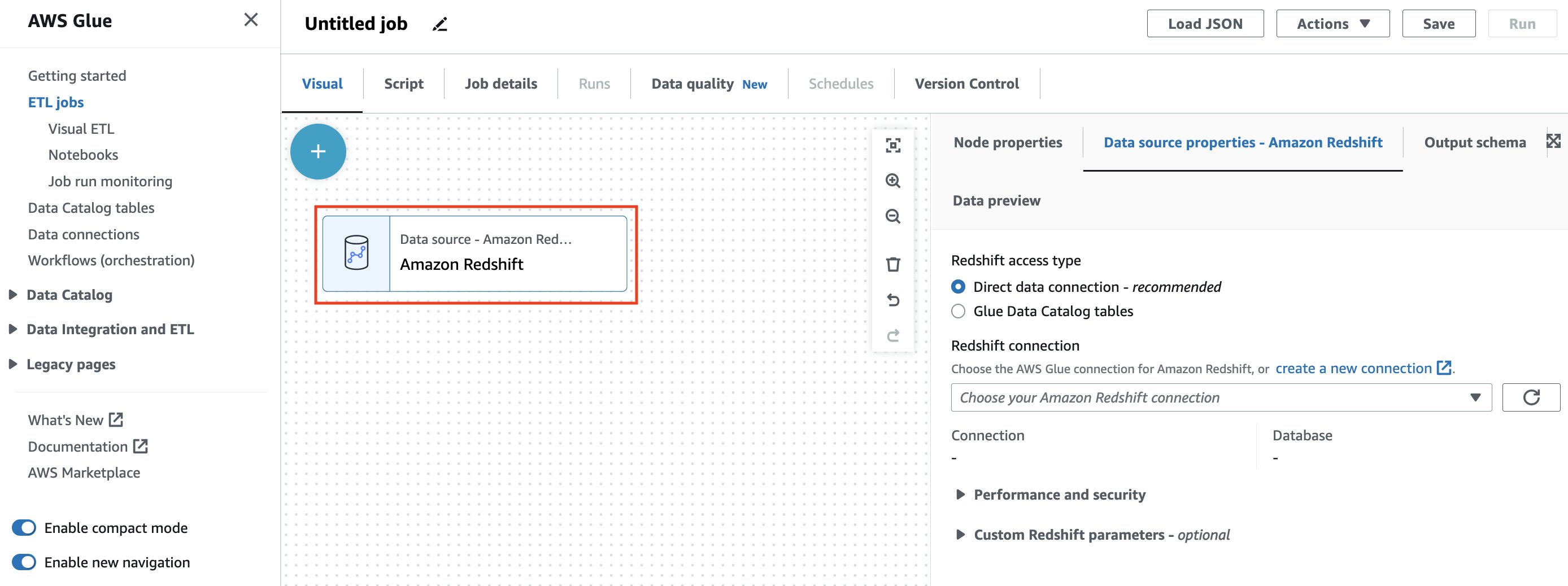
You can choose from two methods of accessing your Amazon Redshift data:
- Direct data connection – This new method allows you to establish a connection to your Amazon Redshift sources without the need to catalog them
- Glue Data Catalog tables – This method requires you to have already crawled or generated your Amazon Redshift tables in the AWS Glue Data Catalog
For this post, we use the Direct data connection option.
- For Redshift access type, select the Direct data connection.
- For Redshift connection, choose your AWS Glue Connection
redshift-demo-blog-connectioncreated in the CloudFormation stack.

Specifying the connection automatically configures all the network related details along with the name of the database you wish to connect to.
The UI then presents a choice on how you’d like to access the data from within your selected Amazon Redshift cluster’s database:
- Choose a single table – This option lets you select a single schema, and a single table from your database. You can browse through all of your available schemas and tables right from the AWS Glue Studio visual editor itself, which makes choosing your source table much easier.

- Enter a custom query – If you’re looking to perform your ETL on a subset of data from your Amazon Redshift tables, you can author an Amazon Redshift query from the AWS Glue Studio UI. This query will be passed to the connected Amazon Redshift cluster, and the returned query result will be available in downstream transformations on AWS Glue Studio.
For the purposes of this post, we write our own custom query that joins data from the preloaded event table and venue table.
- Select Enter a custom query and enter the following query into the query editor:
The intent of this query is to gather the venueid of locations that have had an event between 2008-01-01 14:00:00 and 2008-01-01 15:00:00 and have had venueseats = 0. If we run a similar query from the Amazon Redshift Query Editor, we can see that there are actually five such venues within that time frame. We wish to merge this data back into Amazon Redshift without including these rows.
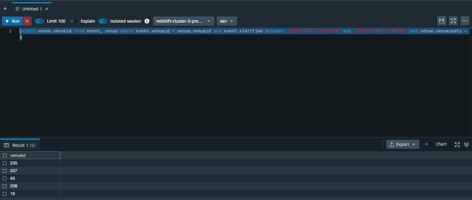
- Choose Infer schema, which allows the AWS Glue Studio visual editor to understand the schema from the returned columns from your query.

You can see the schema on the Output schema tab.
- Under Performance and security, for S3 staging directory, choose the S3 temporary directory location created by the CloudFormation stack ( RedshiftS3TempPath ).
- For IAM role, choose the IAM role specified by RedshiftIamRoleARN in the CloudFormation stack.

Now we’re going to add a transform to drop duplicate rows from our join result. This will ensure that the MERGE operation in the following steps won’t have conflicting keys when performing the operation.
- Choose the Drop Duplicates node to view the node properties.

- On the Transform tab, for Drop duplicates, select Match specific keys.
- For Keys to match rows, choose
venueid.

In this section, we defined the steps to read the output of a custom JOIN query. We then dropped the duplicate records from the returned value. In the next section, we explore the write path on the same job.
Exploring Amazon Redshift writes
Now we go over the enhancements for writing to Amazon Redshift as a destination. This section goes over all the simplified options for writing to Amazon Redshift, but highlights the new Amazon Redshift MERGE capabilities for the purposes of this post.
The MERGE operator offers great flexibility for conditionally merging rows from a source into a destination table. MERGE is powerful because it simplifies operations that traditionally were only achievable by using multiple insert, update, or delete statements separately. Within AWS Glue Studio, particularly with the custom MERGE option, you can define a more complex matching condition to handle finding the records to update.
- From the canvas page of the job used in the previous section, select Amazon Redshift to add an Amazon Redshift node of type Target.

When you close the selector, you should see your Amazon Redshift target node added on the Amazon Glue Studio canvas, along with possible options.
- For Redshift access type, select Direct data connection.
Similar to the Amazon Redshift source node, the Direct data connection method allows you to write directly to your Amazon Redshift tables without needing to have them cataloged within the AWS Glue Data Catalog.
- For Redshift connection, choose your AWS Glue connection
redshift-demo-blog-connectioncreated in the CloudFormation stack.

- For Schema, choose public.

- For Table, choose the venue table as the destination Amazon Redshift table where we will store the merged data.
- Choose MERGE data into target table.
This selection provides the user with two options:
- Choose keys and simple actions – This is a user-friendly version of the MERGE operation. You simply specify the matching keys, and choose what happens to the rows that match the key (update them or delete them) or don’t have any matches (insert them).
- Enter custom MERGE statement – This option provides the most flexibility. You can enter your own custom logic for MERGE.
For this post, we use the simple actions method for performing a MERGE operation.
- For Handling of data and target table, select MERGE data into target table, and then select Choose keys and simple actions.
- For Matching Keys, select
venueid.
This field will become our MERGE condition for checking keys
- For When matched, select the Delete record in the table
- For When not matched, select Insert source data as a new row into the table

With these selections, we’ve configured the AWS Glue job to run a MERGE statement on Amazon Redshift while inserting our data. Moreover, for performing this MERGE operation, we use the as the key (you can select multiple keys). If there is a key match with the destination table’s record, we delete that record. Otherwise, we insert the record into the destination table.
- Navigate to the Job details tab.
- For Name, enter a name for the job.
- For the IAM Role drop down, select the RedshiftIamRole role that was created via the CloudFormation template.
- Choose Save.

- Choose Run and wait for the job to finish.
You can track its progress on the Runs tab.
- After the run reaches a successful state, navigate back to the Amazon Redshift Query Editor.
- Run the same query again to discover that those rows have been deleted in accordance to our MERGE specifications.

In this section, we configured an Amazon Redshift target node to write a MERGE statement to conditionally update records in our destination Amazon Redshift table. We then saved and ran the AWS Glue job, and saw the effect of the MERGE statement on our destination Amazon Redshift table.
Other available write options
In addition to MERGE, the AWS Glue Studio visual editor’s Amazon Redshift destination node also supports a number of other common operations:
- APPEND – Appending to your target table performs an insert into the selected table without updating any of the existing records (if there are duplicates, both records will be retained). In cases where you want to update existing rows in addition to adding new rows (often referred to an UPSERT operation), you can select the Also update existing records in target table option. Note that both APPEND only and UPSERT (APPEND with UPDATE) are a simpler subset of the MERGE functionality discussed earlier.
- TRUNCATE – The TRUNCATE option clears all the data in the existing table but retains all the existing table schema, followed by an APPEND of all new data to the empty table. This option is often used when the full dataset needs to be refreshed and downstream services or tools depend on the table schema being consistent. For example, every night an Amazon Redshift table needs to be fully updated with the latest customer information that will be consumed by an Amazon QuickSight dashboard. In this case, the ETL developer would choose TRUNCATE to ensure the data is fully refreshed but the table schema is guaranteed not to change.
- DROP – This option is used when the full dataset needs to be refreshed and the downstream services or tools that depend on the schema or systems can handle possible schema changes without breaking.
How write operations are being handled on the backend
The Amazon Redshift connector supports two parameters called preactions and postactions. These parameters allow you to run SQL statements that will be passed on to the Amazon Redshift data warehouse before and after the actual write operation is carried out by Spark.
On the Script tab on the AWS Glue Studio page, we can see what SQL statements are being run.
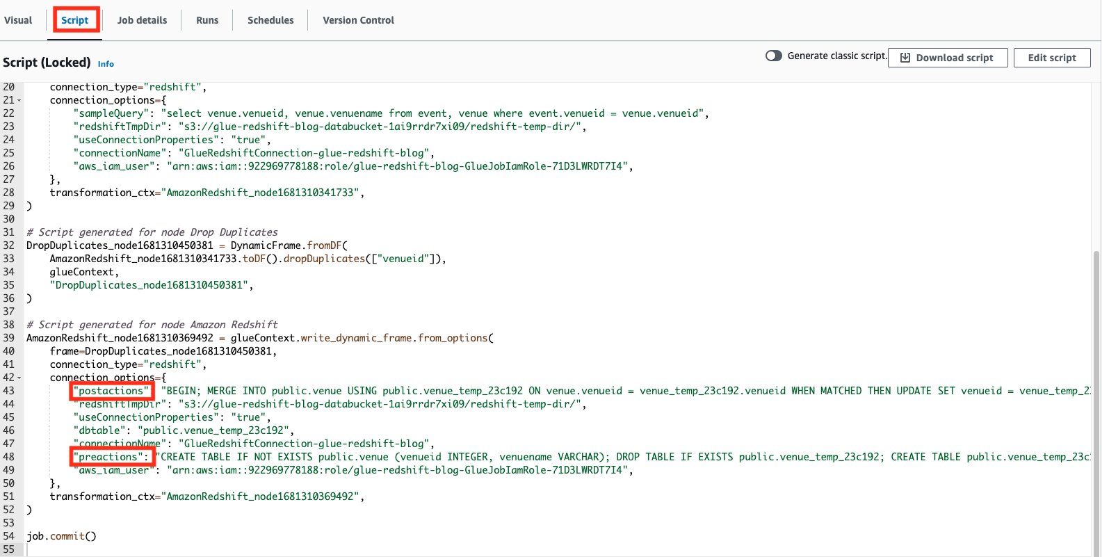
Use a custom implementation for writing data into Amazon Redshift
In the event that the provided presets require more customization, or your use case requires more advanced implementations for writing to Amazon Redshift, AWS Glue Studio also allows you to freely select which preactions and postactions can be run when writing to Amazon Redshift.
To show an example, we create an Amazon Redshift datashare as a preaction, then perform the cleaning up of the same datashare as a postaction via AWS Glue Studio.
NOTE: This section is not executed as part of the above blog and is provided as an example.
- Choose the Amazon Redshift data target node.
- On the Data target properties tab, expand the Custom Redshift parameters section.
- For the parameters, add the following:
- Parameter:
preactionswith ValueBEGIN; CREATE DATASHARE ds1; END - Parameter:
postactionswith ValueBEGIN; DROP DATASHARE ds1; END
- Parameter:
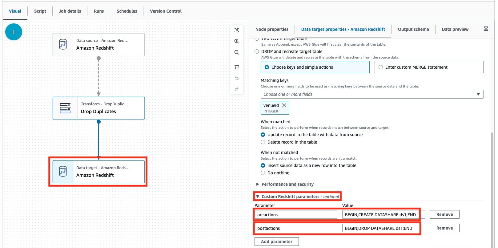
As you can see, we can specify multiple Amazon Redshift statements as a part of both the preactions and postactions parameters. Remember that these statements will override any existing preactions or postactions with your specified actions (as you can see in the following generated code).
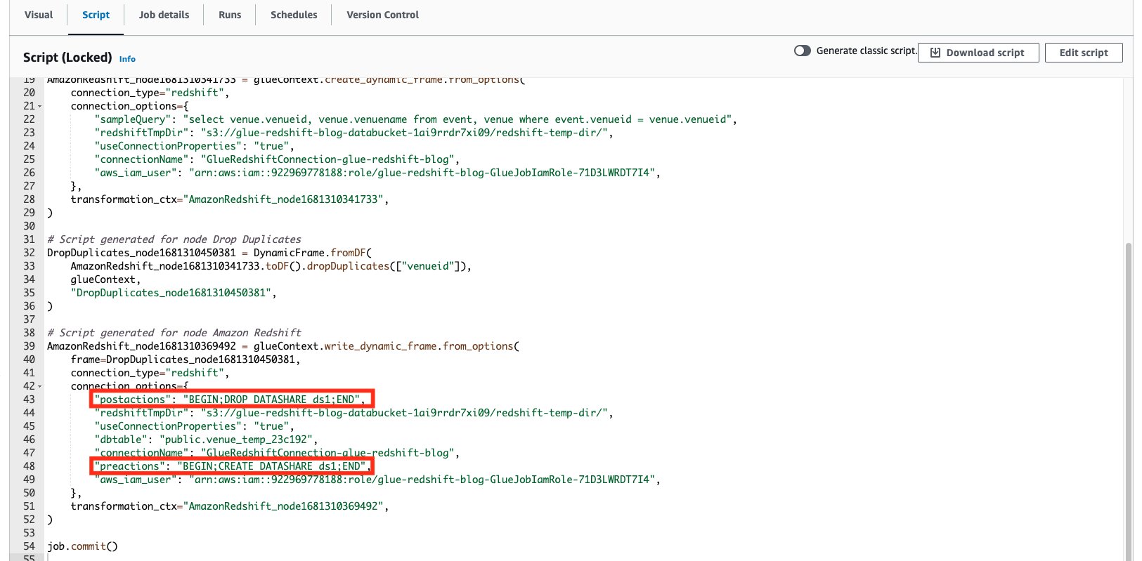
Cleanup
To avoid additional costs, make sure to delete any unnecessary resources and files:
- Empty and delete the contents from the S3 temporary bucket
- If you deployed the sample CloudFormation stack, delete the CloudFormation stack via the AWS CloudFormation console. Make sure to empty the S3 bucket before you delete the bucket.
Conclusion
In this post, we went over the new AWS Glue Studio visual options for performing reads and writes from Amazon Redshift. We also saw the simplicity with which you can browse your Amazon Redshift tables right from the AWS Glue Studio visual editor UI, and how to run your own custom SQL statements against your Amazon Redshift sources. We then explored how to perform simple ETL loading tasks against Amazon Redshift with just a few clicks, and showcased the new Amazon Redshift MERGE statement.
To dive deeper into the new Amazon Redshift integrations for the AWS Glue Studio visual editor, check out Connecting to Redshift in AWS Glue Studio.
About the Authors
Aniket Jiddigoudar is a Big Data Architect on the AWS Glue team. He works with customers to help improve their big data workloads. In his spare time, he enjoys trying out new food, playing video games, and kickboxing.
 Sean Ma is a Principal Product Manager on the AWS Glue team. He has an 18+ year track record of innovating and delivering enterprise products that unlock the power of data for users. Outside of work, Sean enjoys scuba diving and college football.
Every day, customers are challenged with how to manage their growing data volumes and operational costs to unlock the value of data for timely insights and innovation, while maintaining consistent performance. Data creation, consumption, and storage are predicted to grow to 175 zettabytes by 2025, forecasted by the 2022 IDC Global DataSphere report.
As data workloads grow, costs to scale and manage data usage with the right governance typically increase as well. So how do organizational leaders drive their business forward with high performance, controlled costs, and high security? With the right analytics approach, this is possible.
In this post, we look at three key challenges that customers face with growing data and how a modern data warehouse and analytics system like Amazon Redshift can meet these challenges across industries and segments.
Building an optimal data system
As data grows at an extraordinary rate, data proliferation across your data stores, data warehouse, and data lakes can become a challenge. Different departments within an organization can place data in a data lake or within their data warehouse depending on the type of data and usage patterns of that department. Teams may place their unstructured data like social media feeds within their Amazon Simple Storage Service (Amazon S3) data lake and historical structured data within their Amazon Redshift data warehouse. Teams need access to both the data lake and the data warehouse to work seamlessly for best insights, requiring an optimal data infrastructure that can scale almost infinitely to accommodate a growing number of concurrent data users without impacting performance—all while keeping costs under control.
 A quintessential example of a company managing analytics on billions of data points across the data lake and the warehouse in a mission-critical business environment is Nasdaq, an American stock exchange. Within 2 years of migration to Amazon Redshift, Nasdaq was managing 30–70 billion records, growing daily worth over 4 terabytes.
With Amazon Redshift, Nasdaq was able to query their warehouse and use Amazon Redshift Spectrum, a capability to query the data quickly in place without data loading, from their S3 data lakes. Nasdaq minimized time to insights with the ability to query 15 terabytes of data on Amazon S3 immediately without any extra data loading after writing data to Amazon S3. This performance innovation allows Nasdaq to have a multi-use data lake between teams.
Robert Hunt, Vice President of Software Engineering for Nasdaq, shared, “We have to both load and consume the 30 billion records in a time period between market close and the following morning. Data loading delayed the delivery of our reports. We needed to be able to write or load data into our data storage solution very quickly without interfering with the reading and querying of the data at the same time.”
Nasdaq’s massive data growth meant they needed to evolve their data architecture to keep up. They built their foundation of a new data lake on Amazon S3 so they could deliver analytics using Amazon Redshift as a compute layer. Nasdaq’s peak volume of daily data ingestion reached 113 billion records, and they completed data loading for reporting 5 hours faster while running 32% faster queries.
Enabling newer personas with data warehousing and analytics
Another challenge is enabling newer data users and personas with powerful analytics to meet business goals and perform critical decision-making. Where traditionally it was the data engineer and the database administrator who set up and managed the warehouse, today line of business data analysts, data scientists, and developers are all using the data warehouse to get to near-real-time business decision-making.
These personas who don’t have specialized data management or data engineering skills don’t want to be concerned with managing the capacity of their analytics systems to handle unpredictable or spiky data workloads or wait for IT to optimize for cost and capacity. Customers want to get started with analytics on large amounts of data instantly and scale analytics quickly and cost-effectively without infrastructure management.
Take the case of mobile gaming company Playrix. They were able to use Amazon Redshift Serverless to serve their key stakeholders with dashboards with financial data for quick decision-making.
Igor Ivanov, Technical Director of Playrix, stated, “Amazon Redshift Serverless is great for achieving the on-demand high performance that we need for massive queries.”
 Playrix had a two-fold business goal, including marketing to its end-users (game players) with near-real-time data while also analyzing their historical data for the past 4–5 years. In seeking a solution, Playrix wanted to avoid disrupting other technical processes while also increasing cost savings. The company migrated to Redshift Serverless and scaled up to handle more complicated analytics on 600 TB from the past 5 years, all without storing two copies of the data or disrupting other analytics jobs. With Redshift Serverless, Playrix achieved a more flexible architecture and saved an overall 20% in costs of its marketing stack, decreasing its cost of customer acquisition.
“With no overhead and infrastructure management,” Ivanov shared, “we now have more time for experimenting, developing solutions, and planning new research.”
Breaking down data silos
Organizations need to easily access and analyze diverse types of structured and unstructured data, including log files, clickstreams, voice, and video. However, these wide-ranging data types are typically stored in silos across multiple data stores. To unlock the true potential of the data, organizations must break down these silos to unify and normalize all types of data and ensure that the right people have access to the right data.
Data unification can get expensive fast, with time and cost spent on building complex, custom extract, transform, load (ETL) pipelines that move or copy data from system to system. If not done right, you can end up with data latency issues, inaccuracies, and potential security and data governance risks. Instead, teams are looking for ways to share transactionally consistent, live, first-party and third-party data with each other or their end customers, without data movement or data copying.
 Stripe, a payment processing platform for businesses, is an Amazon Redshift customer and a partner with thousands of end customers who require access to Stripe data for their applications. Stripe built the Stripe Data Pipeline, a solution for Stripe customers to access Stripe datasets within their Amazon Redshift data warehouses, without having to build, maintain, or scale custom ETL jobs. The Stripe Data Pipeline is powered by the data sharing capability of Amazon Redshift. Customers get a single source of truth, with low-latency data access, to speed up financial close and get better insights, analyzing best-performing payment methods, fraud by location, and more. Cutting down data engineering time and effort to access unified data creates new business opportunities from comprehensive insights and saves costs.
A modern data architecture with Amazon Redshift
These stories about harnessing maximum value from siloed data across the organization and applying powerful analytics for business insights in a cost-efficient way are possible because of AWS’s approach to a modern data architecture for their customers. Within this architecture, AWS’s data warehousing solution Amazon Redshift is a fully managed petabyte scale system, deeply integrated with AWS database, analytics, and machine learning (ML) services. Tens of thousands of customers use Amazon Redshift every day to run data warehousing and analytics in the cloud and process exabytes of data for business insights. Customers looking for a highly performing, cost-optimized cloud data warehouse solution choose Amazon Redshift for the following reasons:
- Its leadership in price-performance
- The ability to break through data silos for meaningful insights
- Easy analytics capabilities that cut down data engineering and administrative requirements
- Security and reliability features that are offered out of the box, at no additional cost
The price-performance in a cloud data warehouse benchmark metric is simply defined as the cost to perform a particular workload. Knowing how much your data warehouse is going to cost and how performance changes as your user base and data processing increases is crucial for planning, budgeting, and decision-making around choosing the best data warehouse.
Amazon Redshift is able to attain the best price-performance for customers (up to five times better than other cloud data warehouses) by optimizing the code for AWS hardware, high-performance and power-efficient compute hardware, new compression and caching algorithms, and autonomics (ML-based optimizations) within the warehouse to abstract the administrative activities away from the user, saving time and improving performance. Flexible pricing options such as pay-as-you-go with Redshift Serverless, separation of storage and compute scaling, and 1–3-year compute reservations with heavy discounts keep prices low.
The native integrations in Amazon Redshift with databases, data lakes, streaming data services, and ML services, employing zero-ETL approaches help you access data in place without data movement and easily ingest data into the warehouse without building complex pipelines. This keeps data engineering costs low and expands analytics for more users.
For example, the integration in Amazon Redshift with Amazon SageMaker allows data analysts to stay within the data warehouse and create, train, and build ML models in SQL with no need for ETL jobs or learning new languages for ML (see Jobcase Scales ML Workflows to Support Billions of Daily Predictions Using Amazon Redshift ML for an example). Every week, over 80 billion predictions happen in the warehouse with Amazon Redshift ML.
Finally, customers don’t have to pay more to secure their critical data assets. Security features offer comprehensive identity management with data encryption, granular access controls at row and column level, and data masking abilities to protect sensitive data and authorizations for the right users or groups. These features are available out of the box, within the standard pricing model.
Conclusion
Overall, customers who choose Amazon Redshift innovate in a new reality where the data warehouse scales up and down automatically as workloads change, and maximizes the value of data for all cornerstones of their business.
For market leaders like Nasdaq, they are able to ingest billions of data points daily for trading and selling at high volume and velocity, all in time for proper billing and trading the following business day. For customers like Playrix, choosing Redshift Serverless means marketing to customers with comprehensive analytics in near-real time without getting bogged down by maintenance and overhead. For Stripe, it also means taking the complexity and TCO out of ETL, removing silos and unifying data.
Although data will continue to grow at unprecedented amounts, your bottom line doesn’t need to suffer. While organizational leaders face the pressures of solving for cost optimization in all types of economic environments, Amazon Redshift gives market leaders a space to innovate without compromising their data value, performance, and budgets of their cloud data warehouse.
Learn more about maximizing the value of your data with a modern data warehouse like Amazon Redshift. For more information about the price-performance leadership of Amazon Redshift and to review benchmarks against other vendors, see Amazon Redshift continues its price-performance leadership. Additionally, you can optimize costs using a variety of performance and cost levers, including Amazon Redshift’s flexible pricing models, which cover pay-as-you-go pricing for variable workloads, free trials, and reservations for steady state workloads.
About the authors
 Sana Ahmed is a Sr. Product Marketing Manager for Amazon Redshift. She is passionate about people, products and problem-solving with product marketing. As a Product Marketer, she has taken 50+ products to market and worked at various different companies including Sprinklr, PayPal and Facebook. Her hobbies include tennis, museum-hopping and fun conversations with friends and family.

Sunaina AbdulSalah leads product marketing for Amazon Redshift. She focuses on educating customers about the impact of data warehousing and analytics and sharing AWS customer stories. She has a deep background in marketing and GTM functions in the B2B technology and cloud computing domains. Outside of work, she spends time with her family and friends and enjoys traveling.
Data mesh is a new approach to data management. Companies across industries are using a data mesh to decentralize data management to improve data agility and get value from data. However, when a data producer shares data products on a data mesh self-serve web portal, it’s neither intuitive nor easy for a data consumer to know which data products they can join to create new insights. This is especially true in a large enterprise with thousands of data products.
This post shows how to use machine learning (ML) and Amazon Neptune to create automated recommendations to join data products and display those recommendations alongside the existing data products. This allows data consumers to easily identify new datasets and provides agility and innovation without spending hours doing analysis and research.
Background
The success of a data-driven organization recognizes data as a key enabler to increase and sustain innovation. It follows what is called a distributed system architecture. The goal of a data product is to solve the long-standing issue of data silos and data quality. Independent data products often only have value if you can connect them, join them, and correlate them to create a higher order data product that creates additional insights. A modern data architecture is critical in order to become a data-driven organization. It allows stakeholders to manage and work with data products across the organization, enhancing the pace and scale of innovation.
Solution overview
A data mesh architecture starts to solve for the decoupled architecture by decoupling the data infrastructure from the application infrastructure, which is a common challenge in traditional data architectures. It focuses on decentralized ownership, domain design, data products, and self-serve data infrastructure. This allows for a new way of thinking and new organizational elements—namely, a modern data community.
However, today’s data mesh platform contains largely independent data products. Even with well-documented data products, knowing how to connect or join data products is a time-consuming job. Data consumers spend hours, days, or months to understand and analyze the data. Identifying links or relationships between data products is critical to create value from the data mesh and enable a data-driven organization.
The solution in this post illustrates an approach to solving these challenges. It uses a fictional insurance company with several data products shared on their data mesh marketplace. The following figure shows the sample data products used in our solution.

Suppose a consumer is browsing the customer data product in the data mesh marketplace. The consumer wonders if the customer data could be linked to claim, policy, or encounter data. Because these data products come from different lines of business (LOBs) or silos, it’s hard to know. A consumer would have to review each data product and do the necessary analysis and research to know this with any certainty.
To solve this problem, our solution uses ML and Neptune to create recommendations for the data consumer. The solution generates a list of data products, product attributes, and the associated probability scores to show join ability. This reduces the time to discover, analyze, and create new insights.
We use Valentine, a data science algorithm for comparing datasets, to improve data product recommendations. Neptune, the managed AWS graph database service, stores information about explicit connections between datasets, improving the recommendations.
Example use case
Let’s walk through a concrete example. Suppose a consumer is browsing the Customer data product in the data mesh marketplace. Customer is similar to the Policy and Encounter data products, but these products come from different silos. Their similarity to the Customer is hard to gauge. To expedite the consumer’s work, the mesh recommends how the Policy and Encounter products can be connected to the Customer product.

Let’s consider two cases. First, is Customer similar to Claim? The following is a sample of the data in each product.

Intuitively, these two products have lots of overlap. Every Cust\_Nbr in Claim has a corresponding Customer\_ID in Customer. There is no foreign key constraint in Claim that assures us it points to Customer. We think there is enough similarity to infer a join relationship.
The data science algorithm Valentine is an effective tool for this. Valentine is presented in the paper Valentine: Evaluating Matching Techniques for Dataset Discovery (2021, Koutras et al.). Valentine determines if two datasets are joinable or unionable. We focus on the former. Two datasets are joinable if a record from one dataset has a link to a record in the other dataset using one or more columns. Valentine addresses the use case where data is messy: there is no foreign key constraint in place, and data doesn’t match perfectly between datasets. Valentine looks for similarities, and its findings are probabilistic. It scores its proposed matches.
This solution uses an implementation of Valentine available in the following GitHub repo. The first step is to load each data product from its source into a Pandas data frame. If the data is large, load a representative subset of it, at most a few million records. Pass the frames to the valentine\_match() function and select the matching method. We use COMA, one of several methods that Valentine supports. The function’s result indicates the similarity of columns and the score. In this case, it tells us that the Customer\_ID for Customer matches the Cust\_Nbr for Claim, with a very high score. We then instruct the data mesh to recommend Claim to the consumer browsing Customer.

A graph database isn’t required to recommend Claim; the two products could be directly compared. But let’s consider Encounter. Is Customer similar to Encounter? This case is more complicated. Many encounters in the Encounter product don’t link to a customer. An encounter occurs when someone contacts the contact center, which could be by phone or email. The party may or may not be a customer, and if they are a customer, we may not know their customer ID during this encounter. Additionally, sometimes the phone or email they use isn’t the same as the one from a customer record in the Customer product.
In the following sample encounter set, encounters 1 and 2 match to Customer\_ID 4. Note that encounter 2’s inbound\_email doesn’t exactly match the inbound\_email in that customer’s record in the Customer product. Encounter 3 has no Customer\_ID, but its inbound\_email matches the customer with ID 8. Encounter 4 appears to refer to the customer with ID 8, but the email doesn’t match, and no Customer\_ID is given. Encounter 5 only has Inbound\_Phone, but that matches the customer with ID 1. Encounter 6 only has an Inbound\_Phone, and it doesn’t appear to match any of the customers we’ve listed so far.

We don’t have a strong enough comparison to infer similarity.

But we know more about the customer than the Customer product tells us. In the Neptune database, we maintain a knowledge graph that combines multiple products and links them through relationships. A knowledge graph allows us to combine data from different sources to gain a better understanding of a specific problem domain. In Neptune, we combine the Customer product data with an additional data product: Sales Opportunity. We ingest each product from its source into the knowledge graph and model a hasSalesOpportunity relationship between Customer and SalesOpportunity resources. The following figure shows these resources, their attributes, and their relationship.

With the AWS SDK for Pandas, we combine this data by running a query against the Neptune graph. We use a graph query language (such as SPARQL) to wrangle a representative subset of customer and sales opportunity data into a Pandas data frame (shown as Enhanced Customer View in the following figure). In the following example, we enhance customers 7 and 8 with alternate phone or email contact data from sales opportunities.

We pass that frame to Valentine and compare it to Encounter. This time, two additional encounters match a customer.

The score meets our threshold, and is high enough to share with the consumer as a possible match. To the customer browsing Customer in the mesh marketplace, we present the recommendation of Encounter, along with scoring details to support the recommendation. With this recommendation, the consumer can explore the Encounter product with greater confidence.

Conclusion
Data-driven organizations are transitioning to a data product way of thinking. Utilizing strategies like data mesh generates value on a large scale. We took this a step further by creating a blueprint to create smart recommendations by linking similar data products using graph technology and ML. In this post, we showed how an organization can augment a data catalog with additional metadata by using ML and Neptune with an automated process.
This solution solves the interoperability and linkage problem for data products. Additionally, it gives organizations real-time insights, agility, and innovation without spending time on data analysis and research. This approach creates a truly connected ecosystem with simplified access to delight your data consumers. The current solution is platform agnostic; however, in a future post we will show how to implement this using data.all (open-source software) and Amazon DataZone.
To learn more about ML in Neptune, refer to Amazon Neptune ML for machine learning on graphs. You can also explore Neptune notebooks demonstrating ML and data science for graphs. For more information about the data mesh architecture, refer to Design a data mesh architecture using AWS Lake Formation and AWS Glue. To learn more about Amazon DataZone and how you can share, search, and discover data at scale across organizational boundaries.
About the Authors
 Moira Lennox is a Senior Data Strategy Technical Specialist for AWS with 27 years’ experience helping companies innovate and modernize their data strategies to achieve new heights and allow for strategic decision-making. She has experience working in large enterprises and technology providers, in both business and technical roles across multiple industries, including health care live sciences, financial services, communications, digital entertainment, energy, and manufacturing.
 Joel Farvault is Principal Specialist SA Analytics for AWS with 25 years’ experience working on enterprise architecture, data strategy, and analytics, mainly in the financial services industry. Joel has led data transformation projects on fraud analytics, claims automation, and data governance.
 Mike Havey is a Solutions Architect for AWS with over 25 years of experience building enterprise applications. Mike is the author of two books and numerous articles. His Amazon author page
Many customers run big data workloads such as extract, transform, and load (ETL) on Apache Hive to create a data warehouse on Hadoop. Apache Hive has performed pretty well for a long time. But with advancements in infrastructure such as cloud computing and multicore machines with large RAM, Apache Spark started to gain visibility by performing better than Apache Hive.
Customers now want to migrate their Apache Hive workloads to Apache Spark in the cloud to get the benefits of optimized runtime, cost reduction through transient clusters, better scalability by decoupling the storage and compute, and flexibility. However, migration from Apache Hive to Apache Spark needs a lot of manual effort to write migration scripts and maintain different Spark job configurations.
In this post, we walk you through a solution that automates the migration from HiveQL to Spark SQL. The solution was used to migrate Hive with Oozie workloads to Spark SQL and run them on Amazon EMR for a large gaming client. You can also use this solution to develop new jobs with Spark SQL and process them on Amazon EMR. This post assumes that you have a basic understanding of Apache Spark, Hive, and Amazon EMR.
Solution overview
In our example, we use Apache Oozie, which schedules Apache Hive jobs as actions to collect and process data on a daily basis.
We migrate these Oozie workflows with Hive actions by extracting the HQL files, and dynamic and static parameters, and converting them to be Spark compliant. Manual conversion is both time consuming and error prone. To convert the HQL to Spark SQL, you’ll need to sort through existing HQLs, replace the parameters, and change the syntax for a bunch of files.
Instead, we can use automation to speed up the process of migration and reduce heavy lifting tasks, costs, and risks.
We split the solution into two primary components: generating Spark job metadata and running the SQL on Amazon EMR. The first component (metadata setup) consumes existing Hive job configurations and generates metadata such as number of parameters, number of actions (steps), and file formats. The second component consumes the generated metadata from the first component and prepares the run order of Spark SQL within a Spark session. With this solution, we support basic orchestration and scheduling with the help of AWS services like Amazon DynamoDB and Amazon Simple Storage Service (Amazon S3). We can validate the solution by running queries in Amazon Athena.
In the following sections, we walk through these components and how to use these automations in detail.
Generate Spark SQL metadata
Our batch job consists of Hive steps scheduled to run sequentially. For each step, we run HQL scripts that extract, transform, and aggregate input data into one final Hive table, which stores data in HDFS. We use the following Oozie workflow parser script, which takes the input of an existing Hive job and generates configurations artifacts needed for running SQL using PySpark.
Oozie workflow XML parser
We create a Python script to automatically parse the Oozie jobs, including workflow.xml, co-ordinator.xml, job properties, and HQL files. This script can handle many Hive actions in a workflow by organizing the metadata at the step level into separate folders. Each step includes the list of SQLs, SQL paths, and their static parameters, which are input for the solution in the next step.
The process consists of two steps:
- The Python parser script takes input of the existing Oozie Hive job and its configuration files.
- The script generates a metadata JSON file for each step.
The following diagram outlines these steps and shows sample output.

Prerequisites
You need the following prerequisites:
- Python 3.8
- Python packages:
- sqlparse==0.4.2
- jproperties==2.1.1
- defusedxml== 0.7.1
Setup
Complete the following steps:
- Install Python 3.8.
- Create a virtual environment:
- Activate the newly created virtual environment:
- Git clone the project:
- Install dependent packages:
Sample command
We can use the following sample command:
The output is as follows:
Limitations
This method has the following limitations:
- The Python script parses only HiveQL actions from the Oozie workflow.xml.
- The Python script generates one file for each SQL statement and uses the sequence ID for file names. It doesn’t name the SQL based on the functionality of the SQL.
Run Spark SQL on Amazon EMR
After we create the SQL metadata files, we use another automation script to run them with Spark SQL on Amazon EMR. This automation script supports custom UDFs by adding JAR files to spark submit. This solution uses DynamoDB for logging the run details of SQLs for support and maintenance.
Architecture overview
The following diagram illustrates the solution architecture.

Prerequisites
You need the following prerequisites:
- Version:
- Spark 3.X
- Python 3.8
- Amazon EMR 6.1
Setup
Complete the following steps:
- Install the AWS Command Line Interface (AWS CLI) on your workspace by following the instructions in Installing or updating the latest version of the AWS CLI. To configure AWS CLI interaction with AWS, refer to Quick setup.
- Create two tables in DynamoDB: one to store metadata about jobs and steps, and another to log job runs.
- Use the following AWS CLI command to create the metadata table in DynamoDB:
You can check on the DynamoDB console that the table dw-etl-metadata is successfully created.

The metadata table has the following attributes.
| Attributes | Type | Comments |
id | String | partition\_key |
step\_id | String | sort\_key |
step\_name | String | Step description |
sql\_base\_path | string | Base path |
sql\_info | list | List of SQLs in ETL pipeline |
| . | sql\_path | SQL file name |
| . | sql\_active\_flag | y/n |
| . | sql\_load\_order | Order of SQL |
| . | sql\_parameters | Parameters in SQL and values |
spark\_config | Map | Spark configs |
-
- Use the following AWS CLI command to create the log table in DynamoDB:
You can check on the DynamoDB console that the table dw-etl-pipelinelog is successfully created.

The log table has the following attributes.
| Attributes | Type | Comments |
job\_run\_id | String | partition\_key |
id | String | sort\_key (UUID) |
end\_time | String | End time |
error\_description | String | Error in case of failure |
expire | Number | Time to Live |
sql\_seq | Number | SQL sequence number |
start\_time | String | Start time |
Status | String | Status of job |
step\_id | String | Job ID SQL belongs |
The log table can grow quickly if there are too many jobs or if they are running frequently. We can archive them to Amazon S3 if they are no longer used or use the Time to Live feature of DynamoDB to clean up old records.
- Run the first command to set the variable in case you have an existing bucket that can be reused. If not, create a S3 bucket to store the Spark SQL code, which will be run by Amazon EMR.
- Enable secure transfer on the bucket:

- Clone the project to your workspace:
- Create a ZIP file and upload it to the code bucket created earlier:
- Upload the ETL driver code to the S3 bucket:

- Upload sample job SQLs to Amazon S3:

- Add a sample step (
./sample\_oozie\_job\_name/step1/step1.json) to DynamoDB (for more information, refer to Write data to a table using the console or AWS CLI):

- In the Athena query editor, create the database
base:
- Copy the sample data files from the repo to Amazon S3:
- Copy
us\_current.csv:
- Copy

- Copy
states\_current.csv:

- To create the source tables in the base database, run the DDLs present in the repo in the Athena query editor:
- Run the
./sample\_data/ddl/states\_current.qfile by modifying the S3 path to the bucket you created.
- Run the
./sample\_data/ddl/us\_current.qfile by modifying the S3 path to the bucket you created.
- Run the

The ETL driver file implements the Spark driver logic. It can be invoked locally or on an EMR instance.
- Launch an EMR cluster.
- Make sure to select Use for Spark table metadata under AWS Glue Data Catalog settings.

- Add the following steps to EMR cluster.
| Step type | Spark Application |
| Name | Any Name |
| Deploy mode | Client |
| Spark-submit options | --py-files s3://unique-code-bucket-name-#####/framework/code.zip |
| Application location | s3://unique-code-bucket-name-####/framework/etl\_driver.py |
| Arguments | --step\_id sample\_oozie\_job\_name#step1 --job\_run\_id sample\_oozie\_job\_name#step1#2022-01-01-12-00-01 --code\_bucket=s3://unique-code-bucket-name-#######/DW --metadata\_table=dw-etl-metadata --log\_table\_name=dw-etl-pipelinelog --sql\_parameters DATE=2022-02-02::HOUR=12::code\_bucket=s3://unique-code-bucket-name-####### |
| Action on failure | Continue |
The following table summarizes the script arguments.
| Script Argument | Argument Description |
deploy-mode | Spark deploy mode. Client/Cluster. |
name <jobname>#<stepname> | Unique name for the Spark job. This can be used to identify the job on the Spark History UI. |
py-files <s3 path for code>/code.zip | S3 path for the code. |
<s3 path for code>/etl\_driver.py | S3 path for the driver module. This is the entry point for the solution. |
step\_id <jobname>#<stepname> | Unique name for the step. This refers to the step\_id in the metadata entered in DynamoDB. |
job\_run\_id <random UUID> | Unique ID to identify the log entries in DynamoDB. |
log\_table\_name <DynamoDB Log table name> | DynamoDB table for storing the job run details. |
code\_bucket <s3 bucket> | S3 path for the SQL files that are uploaded in the job setup. |
metadata\_table <DynamoDB Metadata table name> | DynamoDB table for storing the job metadata. |
sql\_parameters DATE=2022-07-04::HOUR=00 | Any additional or dynamic parameters expected by the SQL files. |

Validation
After completion of EMR step you should have data on S3 bucket for the table base.states\_daily. We can validate the data by querying the table base.states\_daily in Athena.

Congratulations, you have converted an Oozie Hive job to Spark and run on Amazon EMR successfully.
Solution highlights
This solution has the following benefits:
- It avoids boilerplate code for any new pipeline and offers less maintenance of code
- Onboarding any new pipeline only needs the metadata set up—the DynamoDB entries and SQL to be placed in the S3 path
- Any common modifications or enhancements can be done at the solution level, which will be reflected across all jobs
- DynamoDB metadata provides insight into all active jobs and their optimized runtime parameters
- For each run, this solution persists the SQL start time, end time, and status in a log table to identify issues and analyze runtimes
- It supports Spark SQL and UDF functionality. Custom UDFs can be provided externally to the spark submit command
Limitations
This method has the following limitations:
- The solution only supports SQL queries on Spark
- Each SQL should be a Spark action like insert, create, drop, and so on
In this post, we explained the scenario of migrating an existing Oozie job. We can use the PySpark solution independently for any new development by creating DynamoDB entries and SQL files.
Clean up
Delete all the resources created as part of this solution to avoid ongoing charges for the resources:
- Delete the DynamoDB tables:
- Delete the S3 bucket:
- Stop the EMR cluster if it wasn’t a transient cluster:
Conclusion
In this post, we presented two automated solutions: one for parsing Oozie workflows and HiveQL files to generate metadata, and a PySpark solution for running SQLs using generated metadata. We successfully implemented these solutions to migrate a Hive workload to EMR Spark for a major gaming customer and achieved about 60% effort reduction.
For a Hive with Oozie to Spark migration, these solutions help complete the code conversion quickly so you can focus on performance benchmark and testing. Developing a new pipeline is also quick—you only need to create SQL logic, test it using Spark (shell or notebook), add metadata to DynamoDB, and test via the PySpark SQL solution. Overall, you can use the solution in this post to accelerate Hive to Spark code migration.
About the authors
 Vinay Kumar Khambhampati is a Lead Consultant with the AWS ProServe Team, helping customers with cloud adoption. He is passionate about big data and data analytics.
 Sandeep Singh is a Lead Consultant at AWS ProServe, focused on analytics, data lake architecture, and implementation. He helps enterprise customers migrate and modernize their data lake and data warehouse using AWS services.
 Amol Guldagad is a Data Analytics Consultant based in India. He has worked with customers in different industries like banking and financial services, healthcare, power and utilities, manufacturing, and retail, helping them solve complex challenges with large-scale data platforms. At AWS ProServe, he helps customers accelerate their journey to the cloud and innovate using AWS analytics services.
This is a guest post by Preet Jassi from Alexa Smart Properties.
Alexa Smart Properties (ASP) is powered by a set of technologies that property owners, property managers, and third-party solution providers can use to deploy and manage Alexa-enabled devices at scale. Alexa can simplify tasks like playing music, controlling lights, or communicating with on-site staff. Our team got its start by building products for hospitality and residential properties, but we have since expanded our products to serve senior living and healthcare properties.
With Alexa now available in hotels, hospitals, senior living homes, and other facilities, we hear stories from our customers every day about how much they love Alexa. Everything from helping veterans with visual impairments gain access to information, to enabling a senior living home resident who had fallen and sustained an injury to immediately alert staff. It’s a great feeling when you can say, “The product I work on every day makes a difference in people’s lives!”
Our team builds the software that leading hospitality, healthcare, and senior living facilities use to manage Alexa devices in their properties. We partner directly with organizations that manage their own properties as well as third-party solution providers to provide comprehensive strategy and deployment support for Alexa devices and skills, making sure that they are ready for end-user customers. Our primary goal is to create value for properties through improved customer satisfaction, cost savings, and incremental revenue. We wanted a way to measure that impact in a fast, efficient, easily accessible way from a return on investment (ROI) perspective.
After we had established what capabilities we needed to close our analytics gap, we got in touch with the Amazon QuickSight team to help. In this post, we discuss our requirements and why Amazon QuickSight Embedded was the right fit for what we needed.
Telling the ROI story with data
As a business-to-business-to-consumer product, our team serves the needs of two customers: the end-users who enjoy Alexa-enabled devices at the properties, and the property managers or solution providers that manage the Alexa deployment. We needed to prove to the latter group of customers that deploying Alexa would not only help them delight their customers, but save money as well.
We had the data necessary to tell that ROI story, but we needed an analytics solution that would allow us to provide insights that can be communicated to leadership.
These were our requirements:
- Embeddable dashboards – We wanted to embed analytics into our Alexa Smart Properties management console, used by both enterprise customers and solution providers. With QuickSight, dashboards are embedded for aggregated Alexa usage analytics.
- Easy access to insights – We wanted a tool that was accessible to all of our customers, whether they had a technical background or not. QuickSight provides a beautiful, user-friendly user interface (UI) that our customers can use to interpret their data and analytics.
- Customizable and rich visuals – Our customers needed to be able to dive deep. QuickSight allows you to drill down into the data to easily create and change whatever visuals you need. Our customers love the look of the visuals and how easy it is to share them with their customers.
Analytics drive engagement
With QuickSight, we can now show detailed device usage information, including quantity and frequency, with insights that connect the dots between that engagement and cost savings. For example, property managers can look at total dialog counts to determine that their guests are using Alexa often, which validates their investment.
The following screenshots show an example of the dashboard our solution providers can access, which they can use to send reports to staff at the properties they serve.
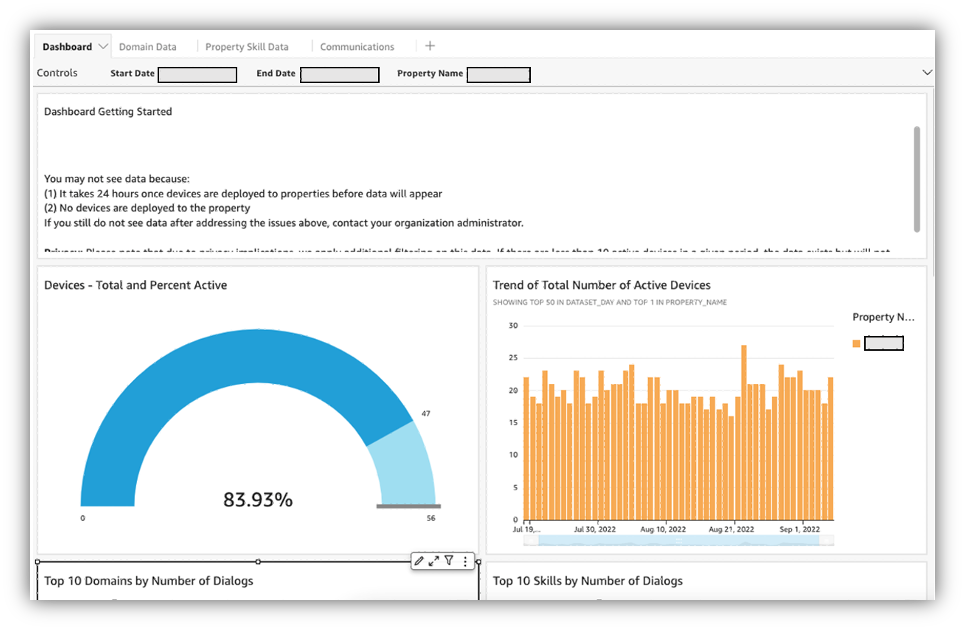
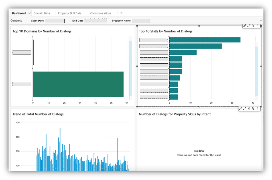
The following screenshots show an example of the Communications tab, which shows how properties use communications features to save costs (both in terms of time and equipment). Customers save time and money on protective equipment by using Alexa’s remote communication features, which enable caretakers to virtually check in on patients instead of visiting a property in person. These metrics help our customers calculate the cost savings from using Alexa.
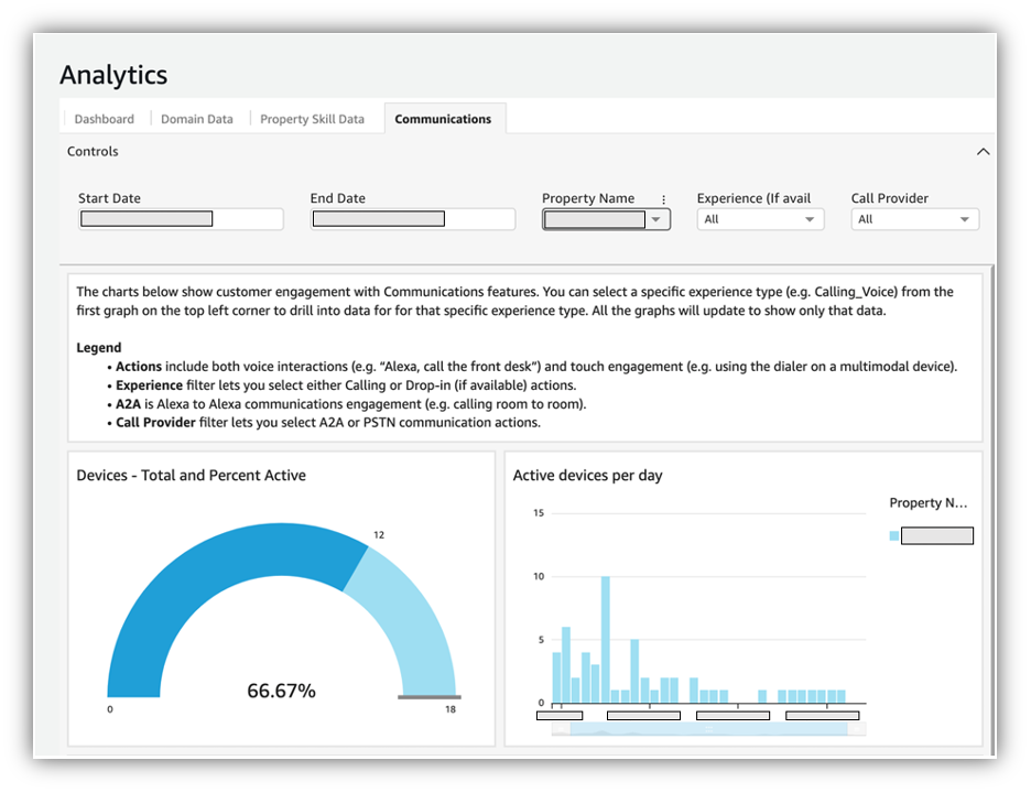
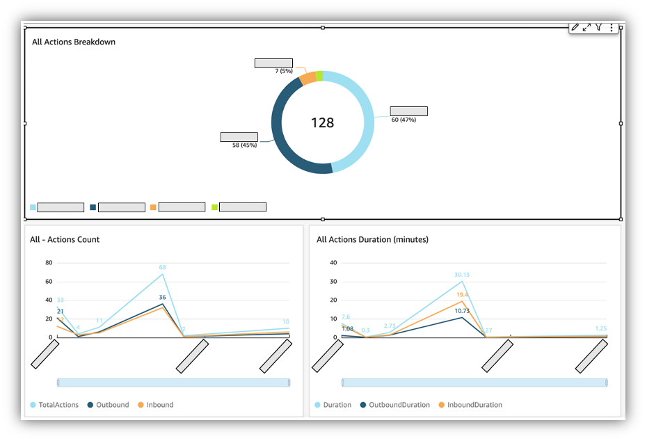
In the last year, the Analytics page in our management console has had over 20,000 page views from customers who are accessing the data and insights there to understand the impact Alexa has had on their businesses.
Insights validate investment
With QuickSight embedded dashboards, our direct-property customers and solution providers now have an easy-to-understand visual representation of how Alexa is making a difference for the guests and patients at each property. Embedded dashboards simplify the viewing, analyzing, and insight gathering for key usage metrics that help both enterprise property owners and solution providers connect the dots between Alexa’s use and money saved. Because we use Amazon Redshift to house our data, QuickSight’s seamless integration made it a fantastic choice.
Going forward, we plan to expand and improve upon the analytics foundation we’ve built with QuickSight by providing programmatic access to data—for example, a CSV file that can be sent to a customer’s Amazon Simple Storage Service (Amazon S3) bucket—as well as adding more data to our dashboards, thereby creating new opportunities for deeper insights.
To learn more about how you can embed customized data visuals, interactive dashboards, and natural language querying into any application, visit Amazon QuickSight Embedded.
About the Author
 Preet Jassi is a Principal Product Manager Technical with Alexa Smart Properties. Preet fell in love with technology in Grade 5 where he built his first website for his elementary school. Prior to completing his MBA at Cornell, Preet was a UI Team Lead with over 6 years of experience as a software engineer post BSc. Preet’s passion is combining his love of technology (specifically analytics and artificial intelligence), with design, and business strategy to build products that customers love, spending time with family, and keeping active. He currently manages the Developer Experience for Alexa Smart Properties focusing on making it quick and easy to deploy Alexa devices in properties and he loves hearing quotes from end customers on how Alexa has changed their lives.
Amazon OpenSearch Serverless is a serverless option of Amazon OpenSearch Service that makes it easy for you to run large-scale search and analytics workloads without having to configure, manage, or scale OpenSearch clusters. It automatically provisions and scales the underlying resources to deliver fast data ingestion and query responses for even the most demanding and unpredictable workloads. With OpenSearch Serverless, you can configure SAML to enable users to access data through OpenSearch Dashboards using an external SAML identity provider (IdP).
AWS IAM Identity Center (Successor to AWS Single Sign-On) helps you securely create or connect your workforce identities and manage their access centrally across AWS accounts and applications, OpenSearch Dashboards being one of them.
In this post, we show you how to configure SAML authentication for OpenSearch Dashboards using IAM Identity Center as its IdP.
Solution overview
The following diagram illustrates how the solution allows users or groups to authenticate into OpenSearch Dashboards using single sign-on (SSO) with IAM Identity Center using its built-in directory as the identity source.

The workflow steps are as follows:
- A user accesses the OpenSearch Dashboard URL in their browser and chooses the SAML provider.
- OpenSearch Serverless redirects the login to the specified IdP.
- The IdP provides a login form for the user to specify the credentials for authentication.
- After the user is authenticated successfully, a SAML assertion is sent back to OpenSearch Serverless.
OpenSearch Serverless validates the SAML assertion, and the user logs in to OpenSearch Dashboards.
Prerequisites
To get started, you must have an active OpenSearch Serverless collection. Refer to Creating and managing Amazon OpenSearch Serverless collections to learn more about creating a collection. Furthermore, you must have the correct AWS Identity and Access Management (IAM) permissions for configuring SAML authentication along with relevant IAM permissions for configuring the data access policy.
IAM Identity Center should be enabled, and you should have the relevant IAM permissions to create an application in IAM Identity Center and create and manage users and groups.
Create and configure the application in IAM Identity Center
To set up your application in IAM Identity Center, complete the following steps:
- On the IAM Identity Center dashboard, choose Applications in the navigation pane.
- Choose Add application

- For Custom application, select Add custom SAML 2.0 application.
- Choose Next.

- Under Configure application, enter a name and description for the application.
- Under IAM Identity Center metadata, choose Download under IAM Identity Center SAML metadata file.

We use this metadata file to create a SAML provider under OpenSearch Serverless. It contains the public certificate used to verify the signature of the IAM Identity Center SAML assertions.
- Under Application properties, leave Application start URL and Relay state blank.
- For Session duration, choose 1 hour (the default value).

Note that the session duration you configure in this step takes precedence over the OpenSearch Dashboards timeout setting specified in the configuration of the SAML provider details on the OpenSearch Serverless end.
- Under Application metadata, select Manually type your metadata values.
- For Application ACS URL, enter your URL using the format
https://collection.<REGION>.aoss.amazonaws.com/\_saml/acs. For example, we enterhttps://collection.us-east-1.aoss.amazonaws.com/\_saml/acsfor this post. - For Application SAML audience, enter your service provider in the format
aws:opensearch:<aws account id>.

- Choose Submit.
Now you modify the attribute settings. The attribute mappings you configure here become part of the SAML assertion that is sent to the application.
- On the Actions menu, choose Edit attribute mappings.

- Configure Subject to map to
${user:email}, with the format unspecified.
Using ${user:email} here ensures that the email address for the user in IAM Identity Center is passed in the <NameId> tag of the SAML response.
- Choose Save changes.

Now we assign a user to the application.
- Create a user in IAM Identity Center to use to log in to OpenSearch Dashboards.
Alternatively, you can use an existing user.
- On the IAM Identity Center console, navigate to your application and choose Assign Users and select the user(s) you would like to assign.

You have now created a custom SAML application. Next, you will configure the SAML provider in OpenSearch Serverless.
Create a SAML provider
The SAML provider you create in this step can be assigned to any collection in the same Region. Complete the following steps:
- On the OpenSearch Service console, under Serverless in the navigation pane, choose SAML authentication under Security.
- Choose Create SAML provider.

- Enter a name and description for your SAML provider.
- Enter the metadata from your IdP that you downloaded earlier.

- Under Additional settings, you can optionally add custom user ID and group attributes. We leave these settings blank for now.
- Choose Create a SAML provider.

You have now configured a SAML provider for OpenSearch Serverless. Next, we walk you through configuring the data access policy for accessing collections.
Create the data access policy
In this section, you set up data access policies for OpenSearch Serverless and allow access to the users. Complete the following steps:
- On the OpenSearch Service console, under Serverless in the navigation pane, choose Data access policies under Security.
- Choose Create access policy.

- Enter a name and description for your access policy.
- For Policy definition method, select Visual Editor.
- In the Rules section, enter a rule name.
- Under Select principals, for Add principals, choose SAML users and groups.

- For SAML provider name, choose the SAML provider you created earlier.

- Specify the user in the format
user/<email>(for example,user/test@example.com).
The value of the email address should match the email address in IAM Identity Center.
- Choose Save.
- Choose Grant and specify the permissions.
You can configure what access you want to provide for the specific user at the collection level and specific indexes at the index pattern level.
You should select the access the user needs based on the least privilege model. Refer to Supported policy permissions and Supported OpenSearch API operations and permissions to set up more granular access for your users.
- Choose Save and configure any additional rules, if required.

You can now review and edit your configuration if needed.
- Choose Create to create the data access policy.

Now you have the data access policy that will allow the users to perform the allowed actions on OpenSearch Dashboards.
Access OpenSearch Dashboards
To sign in to OpenSearch Dashboards, complete the following steps:
- On the OpenSearch Service dashboard, under Serverless in the navigation pane, choose Dashboard.
- Locate your dashboard and copy the OpenSearch Dashboards URL (in the format
<collection-endpoint>/\_dashboards).

- Enter this URL into a new browser tab.
- On the OpenSearch login page, choose your IdP and specify your SSO credentials.
- Choose Login.

Configure SAML authentication using groups in IAM Identity Center
Groups can help you organize your users and permissions in a coherent way. With groups, you can add multiple users from the IdP, and then use groupid as the identifier in the data access policy. For more information, refer to Add groups and Add users to groups.
To configure group access to OpenSearch Dashboards, complete the following steps:
- On the IAM Identity Center console, navigate to your application.
- In the Attribute mappings section, add an additional user as group and map it to
${user:groups}, with the format unspecified. - Choose Save changes.

- For the SAML provider in OpenSearch Serverless, under Additional settings, for Group attribute, enter group.

- For the data access policy, create a new rule or add an additional principal in the previous rule.
- Choose the SAML provider name and enter
group/<GroupId>.

You can fetch the value for the group ID by navigating to the Group section on the IAM Identity Center console.
Clean up
If you don’t want to continue using the solution, be sure to delete the resources you created:
- On the IAM Identity Center console, remove the application.
- On OpenSearch Dashboards, delete the following resources:
Conclusion
In this post, you learned how to set up IAM Identity Center as an IdP to access OpenSearch Dashboards using SAML as SSO. You also learned on how to set up users and groups within IAM Identity Center and control the access of users and groups for OpenSearch Dashboards. For more details, refer to SAML authentication for Amazon OpenSearch Serverless.
Stay tuned for a series of posts focusing on the various options available for you to build effective log analytics and search solutions using OpenSearch Serverless. You can also refer to the Getting started with Amazon OpenSearch Serverless workshop to know more about OpenSearch Serverless.
If you have feedback about this post, submit it in the comments section. If you have questions about this post, start a new thread on the OpenSearch Service forum or contact AWS Support.
About the Authors
 Utkarsh Agarwal is a Cloud Support Engineer in the Support Engineering team at Amazon Web Services. He specializes in Amazon OpenSearch Service. He provides guidance and technical assistance to customers thus enabling them to build scalable, highly available and secure solutions in AWS Cloud. In his free time, he enjoys watching movies, TV series and of course cricket! Lately, he his also attempting to master the art of cooking in his free time – The taste buds are excited, but the kitchen might disagree.
 Ravi Bhatane is a software engineer with Amazon OpenSearch Serverless Service. He is passionate about security, distributed systems, and building scalable services. When he’s not coding, Ravi enjoys photography and exploring new hiking trails with his friends.
Prashant Agrawal is a Sr. Search Specialist Solutions Architect with Amazon OpenSearch Service. He works closely with customers to help them migrate their workloads to the cloud and helps existing customers fine-tune their clusters to achieve better performance and save on cost. Before joining AWS, he helped various customers use OpenSearch and Elasticsearch for their search and log analytics use cases. When not working, you can find him traveling and exploring new places. In short, he likes doing Eat → Travel → Repeat.
This post is co-written by Constantin Scoarță and Horațiu Măiereanu from CyberSolutions Tech.
CyberSolutions is one of the leading ecommerce enablers in Germany. We design, implement, maintain, and optimize award-winning ecommerce platforms end to end. Our solutions are based on best-in-class software like SAP Hybris and Adobe Experience Manager, and complemented by unique services that help automate the pricing and sourcing processes.
We have built data pipelines to process, aggregate, and clean our data for our forecasting service. With the growing interest in our services, we wanted to scale our batch-based data pipeline to process more historical data on a daily basis and yet remain performant, cost-efficient, and predictable. To meet our requirements, we have been exploring the use of Amazon EMR Serverless as a potential solution.
To accelerate our initiative, we worked with the AWS Data Lab team. They offer joint engineering engagements between customers and AWS technical resources to create tangible deliverables that accelerate data and analytics initiatives. We chose to work through a Build Lab, which is a 2–5-day intensive build with a technical customer team.
In this post, we share how we engaged with the AWS Data Lab program to build a scalable and performant data pipeline using EMR Serverless.
Use case
Our forecasting and recommendation algorithm is fed with historical data, which needs to be curated, cleaned, and aggregated. Our solution was based on AWS Glue workflows orchestrating a set of AWS Glue jobs, which worked fine for our requirements. However, as our use case developed, it required more computations and bigger datasets, resulting into unpredictable performance and cost.
This pipeline performs daily extracts from our data warehouse and a few other systems, curates the data, and does some aggregations (such as daily average). Those will be consumed by our internal tools and generate recommendations accordingly. Prior to the engagement, the pipeline was processing 28 days’ worth of historical data in approximately 70 minutes. We wanted to extend that to 100 days and 365 days of data without having to extend the extraction window or factor in the resources configured.
Solution overview
While working with the Data Lab team, we decided to structure our efforts into two approaches. As a short-term improvement, we were looking into optimizing the existing pipeline based on AWS Glue extract, transform, and load (ETL) jobs, orchestrated via AWS Glue workflows. However, for the mid-term to long-term, we looked at EMR Serverless to run our forecasting data pipeline.
EMR Serverless is an option in Amazon EMR that makes it easy and cost-effective for data engineers and analysts to run petabyte-scale data analytics in the cloud. With EMR Serverless, we could run applications built using open-source frameworks such as Apache Spark (as in our case) without having to configure, manage, optimize, or secure clusters. The following factors influenced our decision to use EMR Serverless:
- Our pipeline had minimal dependency on the AWS Glue context and its features, instead running native Apache Spark
- EMR Serverless offers configurable drivers and workers
- With EMR Serverless, we were able to take advantage of its cost tracking feature for applications
- The need for managing our own Spark History Server was eliminated because EMR Serverless automatically creates a monitoring Spark UI for each job
Therefore, we planned the lab activities to be categorized as follows:
- Improve the existing code to be more performant and scalable
- Create an EMR Serverless application and adapt the pipeline
- Run the entire pipeline with different date intervals
The following solution architecture depicts the high-level components we worked with during the Build Lab.

In the following sections, we dive into the lab implementation in more detail.
Improve the existing code
After examining our code decisions, we identified a step in our pipeline that consumed the most time and resources, and we decided to focus on improving it. Our target job for this optimization was the “Create Moving Average” job, which involves computing various aggregations such as averages, medians, and sums on a moving window. Initially, this step took around 4.7 minutes to process an interval of 28 days. However, running the job for larger datasets proved to be challenging – it didn’t scale well and even resulted in errors in some cases.
While reviewing our code, we focused on several areas, including checking data frames at certain steps to ensure that they contained content before proceeding. Initially, we used the count() API to achieve this, but we discovered that head() was a better alternative because it returns the first n rows only and is faster than count() for large input data. With this change, we were able to save around 15 seconds when processing 28 days’ worth of data. Additionally, we optimized our output writing by using coalesce() instead of repartition().
These changes managed to shave off some time, down to 4 minutes per run. However, we could achieve a better performance by using cache() on data frames before performing the aggregations, which materializes the data frame upon the following transformation. Additionally, we used unpersist() to free up executors’ memory after we were done with the mentioned aggregations. This led to a runtime of approximately 3.5 minutes for this job.
Following the successful code improvements, we managed to extend the data input to 100 days, 1 year, and 3 years. For this specific job, the coalesce() function wasn’t avoiding the shuffle operation and caused uneven data distribution per executor, so we switched back to repartition() for this job. By the end, we managed to get successful runs in 4.7, 12, and 57 minutes, using the same number of workers in AWS Glue (10 standard workers).
Adapt code to EMR Serverless
To observe if running the same job in EMR Serverless would yield better results, we configured an application that uses a comparable number of executors as in AWS Glue jobs. In the job configurations, we used 2 cores and 6 GB of memory for the driver and 20 executors with 4 cores and 16 GB of memory. However, we didn’t use additional ephemeral storage (by default, workers come with free 20 GB).
By the time we had the Build Lab, AWS Glue supported Apache Spark 3.1.1; however, we opted to use Spark 3.2.0 (Amazon EMR version 6.6.0) instead. Additionally, during the Build Lab, only x86\_64 EMR Serverless applications were available, although it now also supports arm64-based architecture.
We adapted the code utilizing AWS Glue context to work with native Apache Spark. For instance, we needed to overwrite existing partitions and sync updates with the AWS Glue Data Catalog, especially when old partitions were replaced and new ones were added. We achieved this by setting spark.conf.set("spark.sql.sources.partitionOverwriteMode", "DYNAMIC") and using an MSCK REPAIR query to sync the relevant table. Similarly, we replaced the read and write operations to rely on Apache Spark APIs.
During the tests, we intentionally disabled the fine-grained auto scaling feature of EMR Serverless while running jobs, in order to observe how the code would perform with the same number of workers but different date intervals. We achieved that by setting spark.dynamicAllocation.enabled to disabled (the default is true).
For the same code, number of workers, and data inputs, we managed to get better performance results with EMR Serverless, which were 2.5, 2.9, 6, and 16 minutes for 28 days, 100 days, 1 year, and 3 years, respectively.
Run the entire pipeline with different date intervals
Because the code for our jobs was implemented in a modular fashion, we were able to quickly test all of them with EMR Serverless and then link them together to orchestrate the pipeline via Amazon Managed Workflows for Apache Airflow (Amazon MWAA).
Regarding performance, our previous pipeline using AWS Glue took around 70 minutes to run with our regular workload. However, our new pipeline, powered by Amazon MWAA-backed EMR Serverless, achieved similar results in approximately 60 minutes. Although this is a notable improvement, the most significant benefit was our ability to scale up to process larger amounts of data using the same number of workers. For instance, processing 1 year’s worth of data only took around 107 minutes to complete.
Conclusion and key takeaways
In this post, we outlined the approach taken by the CyberSolutions team in conjunction with the AWS Data Lab to create a high-performing and scalable demand forecasting pipeline. By using optimized Apache Spark jobs on customizable EMR Serverless workers, we were able to surpass the performance of our previous workflow. Specifically, the new setup resulted in 50–72% better performance for most jobs when processing 100 days of data, resulting in an overall cost savings of around 38%.
EMR Serverless applications’ features helped us have better control over cost. For example, we configured the pre-initialized capacity, which resulted in job start times of 1–4 seconds. And we set up the application behavior to start with the first submitted job and automatically stop after a configurable idle time.
As a next step, we are actively testing AWS Graviton2-based EMR applications, which come with more performance gains and lower cost.
About the Authors
 Constantin Scoarță is a Software Engineer at CyberSolutions Tech. He is mainly focused on building data cleaning and forecasting pipelines. In his spare time, he enjoys hiking, cycling, and skiing.
 Horațiu Măiereanu is the Head of Python Development at CyberSolutions Tech. His team builds smart microservices for ecommerce retailers to help them improve and automate their workloads. In his free time, he likes hiking and traveling with his family and friends.
 Ahmed Ewis is a Solutions Architect at the AWS Data Lab. He helps AWS customers design and build scalable data platforms using AWS database and analytics services. Outside of work, Ahmed enjoys playing with his child and cooking.
Amazon EMR on EKS provides a deployment option for Amazon EMR that allows organizations to run open-source big data frameworks on Amazon Elastic Kubernetes Service (Amazon EKS). With EMR on EKS, Spark applications run on the Amazon EMR runtime for Apache Spark. This performance-optimized runtime offered by Amazon EMR makes your Spark jobs run fast and cost-effectively. Also, you can run other types of business applications, such as web applications and machine learning (ML) TensorFlow workloads, on the same EKS cluster. EMR on EKS simplifies your infrastructure management, maximizes resource utilization, and reduces your cost.
We have been continually improving the Spark performance in each Amazon EMR release to further shorten job runtime and optimize users’ spending on their Amazon EMR big data workloads. As of the Amazon EMR 6.5 release in January 2022, the optimized Spark runtime was 3.5 times faster than OSS Spark v3.1.2 with up to 61% lower costs. Amazon EMR 6.10 is now 1.59 times faster than Amazon EMR 6.5, which has resulted in 5.37 times better performance than OSS Spark v3.3.1 with 76.8% cost savings.
In this post, we describe the benchmark setup and results on top of the EMR on EKS environment. We also share a Spark benchmark solution that suits all Amazon EMR deployment options, so you can replicate the process in your environment for your own performance test cases. The solution uses the TPC-DS dataset and unmodified data schema and table relationships, but derives queries from TPC-DS to support the SparkSQL test cases. It is not comparable to other published TPC-DS benchmark results.
Benchmark setup
To compare with the EMR on EKS 6.5 test result detailed in the post Amazon EMR on Amazon EKS provides up to 61% lower costs and up to 68% performance improvement for Spark workloads, this benchmark for the latest release (Amazon EMR 6.10) uses the same approach: a TPC-DS benchmark framework and the same size of TPC-DS input dataset from an Amazon Simple Storage Service (Amazon S3) location. For the source data, we chose the 3 TB scale factor, which contains 17.7 billion records, approximately 924 GB compressed data in Parquet file format. The setup instructions and technical details can be found in the aws-sample repository.
In summary, the entire performance test job includes 104 SparkSQL queries and was completed in approximately 24 minutes (1,397.55 seconds) with an estimated running cost of $5.08 USD. The input data and test result outputs were both stored on Amazon S3.
The job has been configured with the following parameters that match with the previous Amazon EMR 6.5 test:
- EMR release – EMR 6.10.0
- Hardware:
- Compute – 6 X c5d.9xlarge instances, 216 vCPU, 432 GiB memory in total
- Storage – 6 x 900 NVMe SSD build-in storage
- Amazon EBS root volume – 6 X 20GB gp2
- Spark configuration:
- Driver pod – 1 instance among other 7 executors on a shared Amazon Elastic Compute Cloud (Amazon EC2) node:
spark.driver.cores=4spark.driver.memory=5gspark.kubernetes.driver.limit.cores=4.1
- Executor pod – 47 instances distributed over 6 EC2 nodes
spark.executor.cores=4spark.executor.memory=6gspark.executor.memoryOverhead=2Gspark.kubernetes.executor.limit.cores=4.3
- Driver pod – 1 instance among other 7 executors on a shared Amazon Elastic Compute Cloud (Amazon EC2) node:
- Metadata store – We use Spark’s in-memory data catalog to store metadata for TPC-DS databases and tables—
spark.sql.catalogImplementationis set to the default valuein-memory. The fact tables are partitioned by the date column, which consists of partitions ranging from 200–2,100. No statistics are pre-calculated for these tables.
Results
A single test session consists of 104 Spark SQL queries that were run sequentially. We ran each Spark runtime session (EMR runtime for Apache Spark, OSS Apache Spark) three times. The Spark benchmark job produces a CSV file to Amazon S3 that summarizes the median, minimum, and maximum runtime for each individual query.
The way we calculate the final benchmark results (geomean and the total job runtime) are based on arithmetic means. We take the mean of the median, minimum, and maximum values per query using the formula of AVERAGE(), for example AVERAGE(F2:H2). Then we take a geometric mean of the average column I by the formula GEOMEAN(I2:I105) and SUM(I2:I105) for the total runtime.
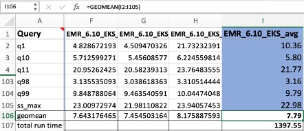
Previously, we observed that EMR on EKS 6.5 is 3.5 times faster than OSS Spark on EKS, and costs 2.6 times less. From this benchmark, we found that the gap has widened: EMR on EKS 6.10 now provides a 5.37 times performance improvement on average and up to 11.61 times improved performance for individual queries over OSS Spark 3.3.1 on Amazon EKS. From the running cost perspective, we see the significant reduction by 4.3 times.

The following graph shows the performance improvement of Amazon EMR 6.10 compared to OSS Spark 3.3.1 at the individual query level. The X-axis shows the name of each query, and the Y-axis shows the total runtime in seconds on logarithmic scale. The most significant performance gains for eight queries (q14a, q14b, q23b, q24a, q24b, q4, q67, q72) demonstrated over 10 times faster for the runtime.

Job cost estimation
The cost estimate doesn’t account for Amazon S3 storage, or PUT and GET requests. The Amazon EMR on EKS uplift calculation is based on the hourly billing information provided by AWS Cost Explorer.
- c5d.9xlarge hourly price – $1.728
- Number of EC2 instances – 6
- Amazon EBS storage per GB-month – $0.10
- Amazon EBS gp2 root volume – 20GB
- Job run time (hour) –
- OSS Spark 3.3.1 – 2.09
- EMR on EKS 6.5.0 – 0.68
- EMR on EKS 6.10.0 – 0.39
| Cost component | OSS Spark 3.3.1 on EKS | EMR on EKS 6.5.0 | EMR on EKS 6.10.0 |
| Amazon EC2 | $21.67 | $7.05 | $4.04 |
| EMR on EKS | $ – | $1.57 | $0.99 |
| Amazon EKS | $0.21 | $0.07 | $0.04 |
| Amazon EBS root volume | $0.03 | $0.01 | $0.01 |
| Total | $21.88 | $8.70 | $5.08 |
Performance enhancements
Although we improve on Amazon EMR’s performance with each release, Amazon EMR 6.10 contained many performance optimizations, making it 5.37 times faster than OSS Spark v3.3.1 and 1.59 times faster than our first release of 2022, Amazon EMR 6.5. This additional performance boost was achieved through the addition of multiple optimizations, including:
- Enhancements to join performance, such as the following:
- Shuffle-Hash Joins (SHJ) are more CPU and I/O efficient than Shuffle-Sort-Merge Joins (SMJ) when the costs of building and probing the hash table, including the availability of memory, are less than the cost of sorting and performing the merge join. However, SHJs have drawbacks, such as risk of out of memory errors due to its inability to spill to disk, which prevents them from being aggressively used across Spark in place of SMJs by default. We have optimized our use of SHJs so that they can be applied to more queries by default than in OSS Spark.
- For some query shapes, we have eliminated redundant joins and enabled the use of more performant join types.
- We have reduced the amount of data shuffled before joins and the potential for data explosions after joins by selectively pushing down aggregates through joins.
- Bloom filters can improve performance by reducing the amount of data shuffled before the join. However, there are cases where bloom filters are not beneficial and can even regress performance. For example, the bloom filter introduces a dependency between stages that reduces query parallelism, but may end up filtering out relatively little data. Our enhancements allow bloom filters to be safely applied to more query plans than OSS Spark.
- Aggregates with high-precision decimals are computationally intensive in OSS Spark. We optimized high-precision decimal computations to increasing their performance.
Summary
With version 6.10, Amazon EMR has further enhanced the EMR runtime for Apache Spark in comparison to our previous benchmark tests for Amazon EMR version 6.5. When running EMR workloads with the the equivalent Apache Spark version 3.3.1, we observed 1.59 times better performance with 41.6% cheaper costs than Amazon EMR 6.5.
With our TPC-DS benchmark setup, we observed a significant performance increase of 5.37 times and a cost reduction of 4.3 times using EMR on EKS compared to OSS Spark.
To learn more and get started with EMR on EKS, try out the EMR on EKS Workshop and visit the EMR on EKS Best Practices Guide page.
About the Authors
 Melody Yang is a Senior Big Data Solution Architect for Amazon EMR at AWS. She is an experienced analytics leader working with AWS customers to provide best practice guidance and technical advice in order to assist their success in data transformation. Her areas of interests are open-source frameworks and automation, data engineering and DataOps.
 Ashok Chintalapati is a software development engineer for Amazon EMR at Amazon Web Services.
This is a guest post by Carl Marrelli from SANS Institute.
The SANS Institute is a world leader in cybersecurity training and certification. For over 30 years, SANS has worked with leading organizations to help ensure security across their organization, as well as with individual IT professionals who want to build and grow their security careers. We partner with over 500 organizations and support over 200,000 IT professionals with more than 90 technical training courses and over 40 professional (GIAC) certifications.
Our Security Awareness products include more than 70 instructional modules and have been deployed to over 6.5 million end-users to bring cybersecurity training to each employee within an organization.
As the Security Awareness department in particular began developing product strategies to deliver data-driven insights to customers, we were clear on using existing analytics services to rapidly build customer-facing analytics solutions. Building on a proven cloud provider would allow us to focus on our core expertise of helping organizations train, learn, and mature their programs instead of spending extra time and resources building and maintaining analytics from scratch.
We identified Amazon QuickSight, a fully managed, cloud-native business intelligence (BI) service, as the product that fit all our criteria. With it, we found an intuitive product with rich visualizations that we could build and grow with rapidly, allowing us to innovate without monetary risks or being locked in to cumbersome contracts. We considered other options, but they couldn’t support the licensing model that fit our needs.
In this post, we go over how we use QuickSight to serve our security customers.
Helping manage human risk with data-driven insights
SANS Security Awareness helps organizations use best-in-class security awareness and training solutions to transform their ability to measure and manage human risk. Security awareness programs are initiatives aimed at educating individuals about the importance of information security and the best practices for maintaining the confidentiality, integrity, and availability of information. We deliver expertly authored training materials to organizations, including computer-based video training sessions, interactive learning modules, supplemental materials, and reinforcement curriculum to keep security top-of-mind for all employees.
As organizations rapidly adopt and expand their use of digital technologies in their day-to-day work, the number of touchpoints with humans increases. As threat landscapes become increasingly more severe, managing human risk is critical to the success of the security program in any organization. Not only do organizations have to conduct security awareness training programs, but they also need insights into data and metrics that identify points of weakness to take data-driven corrective courses of action. As a leader in the space, we wanted to innovate by bringing relevant data-driven insights to our Security Awareness partners and customers in the journey to ensuring human-centered security across their organizations.
New data products to enhance and gamify risk assessment
We built one of our first insights products to support our Behavioral Risk Assessment. This service allows senior security and risk leaders to assess human risk with data handling, digital behavior, and compliance in an organization by individual, team, geography, business unit, and more. Leaders use the assessment to mature their security awareness capability with risk-informed interventions, identify process and procedure gaps, surface shadow IT, and reduce overall awareness training costs by focusing attention on the most important areas of risk.

Delivered via a survey customized to the data types and risk profile of an organization, this assessment allows risk management leaders to more easily understand the data handling practices across roles and departments. Dashboards built in QuickSight empower stakeholders to quickly visualize what areas may need added attention by way of training intervention or updated policy.
Another product area where we invested in analytics to help organizations identify human risk is in gamified awareness training. The SANS Scavenger Hunt utilizes QuickSight in a unique way as a real-time game scoreboard. Players compete in the hunt while solving cybersecurity-related challenges, giving security teams a fun way to engage the workforce and promote good cyber behaviors.
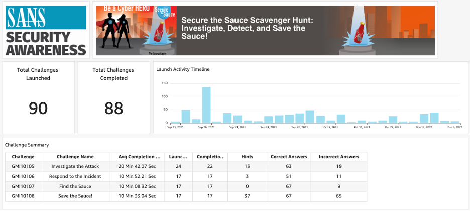
The Scavenger Hunt was widely deployed during global Cybersecurity Awareness Month—a time for security awareness practitioners to shine a light on the purpose and mission of security awareness and also have a little fun. Typically, programs run during this time take place outside any regulated training cycle and are typically not delivered as mandatory training. This being the case, we identified dashboards as a way to gamify the experience to increase engagement among participants. These dashboards, built using QuickSight, provided users access to a leaderboard to not only track their own progress, but to also see how they compared to their fellow participants.
Building on the success of their experience with QuickSight and the Scavenger Hunt, we wanted to push the gamification and dashboards concept further so Chief Information and Security Officers (CISOs) and security teams could identify and mitigate the human side of ransomware risk. We developed Snack Attack!, a gamified learning experience that shows an organization how employees are performing in six key defensive areas where ransomware can be prevented. In 2021, over 80% of cyber breaches involved human error of some kind. Employees must have a fundamental awareness of cybersecurity and the ability to apply cyber knowledge within the scope of their jobs. Snack Attack! and QuickSight proved to be a great product to visualize and action on areas of human risk and sentiment for senior leadership.
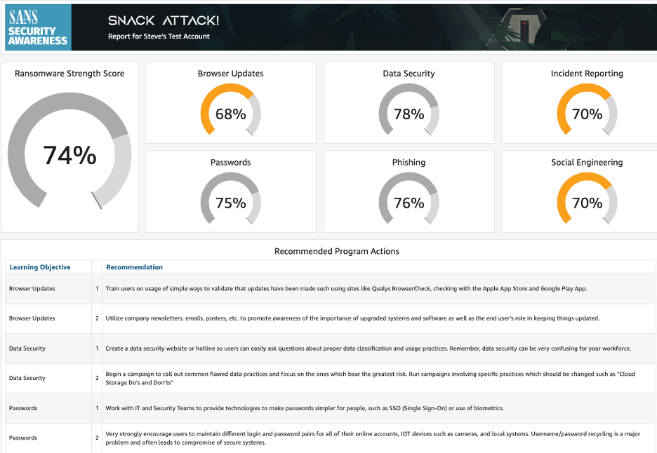
With Snack Attack!, we looked at Cybersecurity Awareness Month from the viewpoint of the awareness practitioner. The program itself focuses on driving engagement through an entertaining storyline with creative visuals. We chose to use the data from the training to help our customers build their awareness programs going forward. The dashboards included in Snack Attack! give the security awareness practitioner insights into the learned behavior of their users. Quick visualizations of learners’ scoring in Snack Attack! can act as an audit of the effectiveness of their existing program and provide a roadmap for future trainings.
Paving the way in using analytics for customer security
The SANS Institute brings together security awareness training programs with a metrics-based approach through out-of-the-box analytics dashboards so our customers can assess and manage human risk successfully. With QuickSight, we were able to rapidly innovate, developing valuable data products at a speed we could not have otherwise. Without up-front investments to get started and with the low cost to try with usage-based pricing, we were able to quickly ideate, build, and deploy customer-facing analytic products to drive security awareness within our customer organizations. Our analytics solutions differentiate us from existing enterprise products. With QuickSight, we are able to show organizations where they have cyber risk.
With the delivery of analytics solutions to customers, the SANS Institute is not only a top cybersecurity training, learning, and certification platform, but also a technology provider that helps customers use data and insights to make meaningful change in their organization. Moving forward, we have identified an expansion of QuickSight dashboards into our larger suite of assessments as the next logical step. Along with the Behavioral Risk Assessment, we offer Knowledge and Culture assessments to help security awareness practitioners better understand where and how to apply training and gauge the effectiveness of their programs. Because of the success we have had with QuickSight on our existing projects, we feel that similar dashboards can provide even more value to our customers.
To learn more about how QuickSight can help your business with dashboards, reports, and more, visit Amazon QuickSight.
About the Author
 Carl R. Marrelli is the Director of Business Development and Digital Programs at SANS Institute. Based in Charlotte, NC, he has extensive experience in cross-functional team leadership, product management, and product marketing. Previously as Head of Product at SANS, Carl led the product management team for the Online Training and Security Awareness divisions through a significant growth period. Carl’s unique perspective and innovative ideas, support SANS as the company continues its mission to empower cybersecurity practitioners around the world.
Inventory management is a critical function for any business that deals with physical products. The primary challenge businesses face with inventory management is balancing the cost of holding inventory with the need to ensure that products are available when customers demand them.
The consequences of poor inventory management can be severe. Overstocking can lead to increased holding costs and waste, while understocking can result in lost sales, reduced customer satisfaction, and damage to the business’s reputation. Inefficient inventory management can also tie up valuable resources, including capital and warehouse space, and can impact profitability.
Forecasting is another critical component of effective inventory management. Accurately predicting demand for products allows businesses to optimize inventory levels, minimize stockouts, and reduce holding costs. However, forecasting can be a complex process, and inaccurate predictions can lead to missed opportunities and lost revenue.
To address these challenges, businesses need an inventory management and forecasting solution that can provide real-time insights into inventory levels, demand trends, and customer behavior. Such a solution should use the latest technologies, including Internet of Things (IoT) sensors, cloud computing, and machine learning (ML), to provide accurate, timely, and actionable data. By implementing such a solution, businesses can improve their inventory management processes, reduce holding costs, increase revenue, and enhance customer satisfaction.
In this post, we discuss how to streamline inventory management forecasting systems with AWS managed analytics, AI/ML, and database services.
Solution overview
In today’s highly competitive business landscape, it’s essential for retailers to optimize their inventory management processes to maximize profitability and improve customer satisfaction. With the proliferation of IoT devices and the abundance of data generated by them, it has become possible to collect real-time data on inventory levels, customer behavior, and other key metrics.
To take advantage of this data and build an effective inventory management and forecasting solution, retailers can use a range of AWS services. By collecting data from store sensors using AWS IoT Core, ingesting it using AWS Lambda to Amazon Aurora Serverless, and transforming it using AWS Glue from a database to an Amazon Simple Storage Service (Amazon S3) data lake, retailers can gain deep insights into their inventory and customer behavior.
With Amazon Athena, retailers can analyze this data to identify trends, patterns, and anomalies, and use Amazon ElastiCache for customer-facing applications with reduced latency. Additionally, by building a point of sales application on Amazon QuickSight, retailers can embed customer 360 views into the application to provide personalized shopping experiences and drive customer loyalty.
Finally, we can use Amazon SageMaker to build forecasting models that can predict inventory demand and optimize stock levels.
With these AWS services, retailers can build an end-to-end inventory management and forecasting solution that provides real-time insights into inventory levels and customer behavior, enabling them to make informed decisions that drive business growth and customer satisfaction.
The following diagram illustrates a sample architecture.

With the appropriate AWS services, your inventory management and forecasting system can have optimized collection, storage, processing, and analysis of data from multiple sources. The solution includes the following components.
Data ingestion and storage
Retail businesses have event-driven data that requires action from downstream processes. It’s critical for an inventory management application to handle the data ingestion and storage for changing demands.
The data ingestion process is typically triggered by an event such as an order being placed, kicking off the inventory management workflow, which requires actions from backend services. Developers are responsible for the operational overhead of trying to maintain the data ingestion load from an event driven-application.
The volume and velocity of data can change in the retail industry each day. Events like Black Friday or a new campaign can create volatile demand in what is required to process and store the inventory data. Serverless services designed to scale to businesses’ needs help reduce the architectural and operational challenges that are driven from high-demand retail applications.
Understanding the scaling challenges that occur when inventory demand spikes, we can deploy Lambda, a serverless, event-driven compute service, to trigger the data ingestion process. As inventory events occur like purchases or returns, Lambda automatically scales compute resources to meet the volume of incoming data.
After Lambda responds to the inventory action request, the updated data is stored in Aurora Serverless. Aurora Serverless is a serverless relational database that is designed to scale to the application’s needs. When peak loads hit during events like Black Friday, Aurora Serverless deploys only the database capacity necessary to meet the workload.
Inventory management applications have ever-changing demands. Deploying serverless services to handle the ingestion and storage of data will not only optimize cost but also reduce the operational overhead for developers, freeing up bandwidth for other critical business needs.
Data performance
Customer-facing applications require low latency to maintain positive user experiences with microsecond response times. ElastiCache, a fully managed, in-memory database, delivers high-performance data retrieval to users.
In-memory caching provided by ElastiCache is used to improve latency and throughput for read-heavy applications that online retailers experience. By storing critical pieces of data in-memory like commonly accessed product information, the application performance improves. Product information is an ideal candidate for a cached store due to data staying relatively the same.
Functionality is often added to retail applications to retrieve trending products. Trending products can be cycled through the cache dependent on customer access patterns. ElastiCache manages the real-time application data caching, allowing your customers to experience microsecond response times while supporting high-throughput handling of hundreds of millions of operations per second.
Data transformation
Data transformation is essential in inventory management and forecasting solutions for both data analysis around sales and inventory, as well as ML for forecasting. This is because raw data from various sources can contain inconsistencies, errors, and missing values that may distort the analysis and forecast results.
In the inventory management and forecasting solution, AWS Glue is recommended for data transformation. The tool addresses issues such as cleaning, restructuring, and consolidating data into a standard format that can be easily analyzed. As a result of the transformation, businesses can obtain a more precise understanding of inventory, sales trends, and customer behavior, influencing data-driven decisions to optimize inventory management and sales strategies. Furthermore, high-quality data is crucial for ML algorithms to make accurate forecasts.
By transforming data, organizations can enhance the accuracy and dependability of their forecasting models, ultimately leading to improved inventory management and cost savings.
Data analysis
Data analysis has become increasingly important for businesses because it allows leaders to make informed operational decisions. However, analyzing large volumes of data can be a time-consuming and resource-intensive task. This is where Athena come in. With Athena, businesses can easily query historical sales and inventory data stored in S3 data lakes and combine it with real-time transactional data from Aurora Serverless databases.
The federated capabilities of Athena allow businesses to generate insights by combining datasets without the need to build ETL (extract, transform, and load) pipelines, saving time and resources. This enables businesses to quickly gain a comprehensive understanding of their inventory and sales trends, which can be used to optimize inventory management and forecasting, ultimately improving operations and increasing profitability.
With Athena’s ease of use and powerful capabilities, businesses can quickly analyze their data and gain valuable insights, driving growth and success without the need for complex ETL pipelines.
Forecasting
Inventory forecasting is an important aspect of inventory management for businesses that deal with physical products. Accurately predicting demand for products can help optimize inventory levels, reduce costs, and improve customer satisfaction. ML can help simplify and improve inventory forecasting by making more accurate predictions based on historical data.
SageMaker is a powerful ML platform that you can use to build, train, and deploy ML models for a wide range of applications, including inventory forecasting. In this solution, we use SageMaker to build and train an ML model for inventory forecasting, covering the basic concepts of ML, the data preparation process, model training and evaluation, and deploying the model for use in a production environment.
The solution also introduces the concept of hierarchical forecasting, which involves generating coherent forecasts that maintain the relationships within the hierarchy or reconciling incoherent forecasts. The workshop provides a step-by-step process for using the training capabilities of SageMaker to carry out hierarchical forecasting using synthetic retail data and the scikit-hts package. The FBProphet model was used along with bottom-up and top-down hierarchical aggregation and disaggregation methods. We used Amazon SageMaker Experiments to train multiple models, and the best model was picked out of the four trained models.
Although the approach was demonstrated on a synthetic retail dataset, you can use the provided code with any time series dataset that exhibits a similar hierarchical structure.
Security and authentication
The solution takes advantage of the scalability, reliability, and security of AWS services to provide a comprehensive inventory management and forecasting solution that can help businesses optimize their inventory levels, reduce holding costs, increase revenue, and enhance customer satisfaction. By incorporating user authentication with Amazon Cognito and Amazon API Gateway, the solution ensures that the system is secure and accessible only by authorized users.
Next steps
The next step to build an inventory management and forecasting solution on AWS would be to go through the Inventory Management workshop. In the workshop, you will get hands-on with AWS managed analytics, AI/ML, and database services to dive deep into an end-to-end inventory management solution. By the end of the workshop, you will have gone through the configuration and deployment of the critical pieces that make up an inventory management system.
Conclusion
In conclusion, building an inventory management and forecasting solution on AWS can help businesses optimize their inventory levels, reduce holding costs, increase revenue, and enhance customer satisfaction. With AWS services like IoT Core, Lambda, Aurora Serverless, AWS Glue, Athena, ElastiCache, QuickSight, SageMaker, and Amazon Cognito, businesses can use scalable, reliable, and secure technologies to collect, store, process, and analyze data from various sources.
The end-to-end solution is designed for individuals in various roles, such as business users, data engineers, data scientists, and data analysts, who are responsible for comprehending, creating, and overseeing processes related to retail inventory forecasting. Overall, an inventory management and forecasting solution on AWS can provide businesses with the insights and tools they need to make data-driven decisions and stay competitive in a constantly evolving retail landscape.
About the Authors
 Jason D’Alba is an AWS Solutions Architect leader focused on databases and enterprise applications, helping customers architect highly available and scalable solutions.
 Navnit Shukla is an AWS Specialist Solution Architect, Analytics, and is passionate about helping customers uncover insights from their data. He has been building solutions to help organizations make data-driven decisions.
 Vetri Natarajan is a Specialist Solutions Architect for Amazon QuickSight. Vetri has 15 years of experience implementing enterprise business intelligence (BI) solutions and greenfield data products. Vetri specializes in integration of BI solutions with business applications and enable data-driven decisions.
 Sindhura Palakodety is a Solutions Architect at AWS. She is passionate about helping customers build enterprise-scale Well-Architected solutions on the AWS platform and specializes in Data Analytics domain.
Happy birthday Amazon QuickSight Community! We are celebrating 1 year since the launch of our new Community. The Amazon QuickSight Community website is a one-stop-shop where business intelligence (BI) authors and developers from across the globe can ask and answer questions, stay up to date, network, and learn together about Amazon QuickSight. In this post, we celebrate the rapid growth of our first year of the QuickSight Community, discuss new Community features, and share voices from our Community. We also invite you to sign up for the QuickSight Community (it’s easy and free) and get started on your learning journey.

We’re growing strong
Since last year’s announcement of the new QuickSight Community, we are witnessing hundreds of thousands of visits to the QuickSight Community each month. Answers to thousands of searchable questions have been posted, and our online Learning Series is now running every week. An events calendar has been added, and hundreds of learning resources have been posted (how-to videos and articles, Getting Started resources, blog posts, and What’s New posts). Furthermore, a Community Manager has been brought on board. And Community Experts and QuickSight Solution Architects are posting robust answers in the Q&A, supported by AWS Professional Services, AWS Data Lab, and Amazon QuickSight Service Delivery Partners—led by West Loop Strategy. In addition, other QuickSight Partners and content creators are bringing new life to the Community.

New QuickSight Community members at an internal Amazon conference
Why are we excited? Community members share their voices
As we celebrate year one, QuickSight Community members share their voices:
“The community has been an awesome space to exchange ideas, problems, and solutions, which has really helped every one of us in adopting QuickSight more effectively!” #thank you #community — Sagnik Mukherjee, Data and Analytics Architect, QuickSight Expert
“I am so excited for the QuickSight Learning Series! And I am happy to know that there is a supportive community…as I begin my QS journey!“ — Rachel Krentz, Configuration Analyst, Madaket
“The community has evolved so much in just one year!” — Darren Demicoli, BI Team Lead, The Mill Adventure, QuickSight Expert
“Happy Birthday QuickSight Community! I’m pretty new here but have found this to be a really great resource with answers to every question I have been able to come up with so far. Cheers!” — Brian Jager, Sales Operations Lead, Amazon Business
“I love being connected directly with other users and solutions architects…The QuickSight Community helps me out a ton not having to spend as much of my time on training when I can point new users to a resource where their questions have likely already been answered.” — Ryane Brady, Programmer Analyst, GROWMARK, Inc., QuickSight Expert
Hear more voices from our Community on our birthday post.
The QuickSight Community: Your one-stop-shop for BI learning
Here’s a quick tour of the QuickSight Community website as well as its new features.
The following figure shows the homepage view and everything that’s available.

Learning Center: What’s new
In addition to growing a robust, searchable Q&A, in the last year, we’ve added tons of new learning resources to the QuickSight Community, including:
- Getting Started resources and Embedded Analytics resources
- New how-to articles
- Weekly learning series and workshop videos
When you select Learning Center on the homepage, you can choose from these various resources.

New: Learning events
In the last year, we’ve added an Events section to the QuickSight Community. We now offer weekly and monthly learning webinars as well as featured in-person and online events. Ongoing virtual events include:
- QuickSight Learning Series – Weekly (Wednesdays and Thursdays: Americas and Europe-friendly times)
- AWS PartnerCast Series on new QuickSight features – Monthly (first Fridays)
- Virtual Immersion Days – Amazon QuickSight – Monthly (second and third Wednesdays)
- Live Q&A with Solution Architects – Monthly (fourth Thursdays)
New: Experts and user groups
We’ve been excited to see QuickSight user groups pop up over the past year, including one in the Twin Cities and one in Chicago—both hosted by QuickSight Service Delivery Partners (Charter Solutions and West Loop Strategy, respectively).
In addition, we’ve launched our QuickSight Experts program, honoring top question-answerers in the Community. These rock stars have relentlessly helped their peers take their learning to the next level.

Ryane Brady, Programmer Analyst, GROWMARK, Inc., is a QuickSight Expert and top question-answerer in the Community. Here she is showing off her Expert swag. See the 2022 to Q1 2023 list of Experts at the bottom of this post.
First External Viz Challenge
In the last year, AWS hosted its very first external data visualization design competition to invited QuickSight Service Delivery Partners. This enabled QuickSight Partners to show off their visual analytics and storytelling skills. We were proud to feature the QuickSight Partner Viz Challenge winners of 2022 on the QuickSight Community.

Want to be a part of the QuickSight Community?
| Sign up now to join the QuickSight Community (it’s free and easy) and take your QuickSight learning to the next level. |
As part of the Community, you can:
- Encourage your teams and colleagues to create QuickSight Community user profiles—signup up is easy
- Click the bell icon in the top right corner of the page to get notifications and keep up to date with QuickSight news
- Share your community ideas with the Community Manager
Come in on the ground floor and help us take the QuickSight Community to the next level:
- Become an Expert and share your knowledge
- Pioneer a user group online or in your area
- Contribute a how-to article
If you’re interested in any of these opportunities, reach out to Kristin, the Sr. Online Community Manager for QuickSight, at kmandia@amazon.com.
We’re just getting started
Thank you to everyone who has helped the QuickSight Community grow over the last year! We can’t wait to see what this next year has in store!
Special thanks to our QuickSight Experts who make the QuickSight Community possible (listed alphabetically): Ryane Brady, Biswajit Dash, Darren Demicoli, Max Engelhard, Charles Greenacre, Naveed Hashimi, Todd Hoffman, Mike Khuns, Thomas Kotzurek, Sanjeeb Mohapatra, Sagnik Mukherjee and David Wong. Incredible gratitude to Lillie Atkins and Mia Heard, who launched the Community a year ago. Also, thanks to Jose Kunnackal John, Jill Florant, the QuickSight Solution Architects, Amazon QuickSight Service Delivery Partners—led by West Loop Strategy, AWS Service Acceleration team, AWS ProServe team, and AWS Data Lab team for your incredible investment in the QuickSight Community.
About the Authors
 Kristin Mandia is Senior Online Community Manager for Amazon QuickSight, Amazon Web Service’s cloud-native, fully managed BI service.
 Ian McNamara is a Program Manager and writer on the Customer Success Team for Amazon QuickSight, Amazon Web Service’s cloud-native, fully managed BI service.
Amazon EMR is a big data service offered by AWS to run Apache Spark and other open-source applications on AWS to build scalable data pipelines in a cost-effective manner. Monitoring the logs generated from the jobs deployed on EMR clusters is essential to help detect critical issues in real time and identify root causes quickly.
Pushing those logs into Amazon CloudWatch enables you to centralize and drive actionable intelligence from your logs to address operational issues without needing to provision servers or manage software. You can instantly begin writing queries with aggregations, filters, and regular expressions. In addition, you can visualize time series data, drill down into individual log events, and export query results to CloudWatch dashboards.
To ingest logs that are persisted on the Amazon Elastic Compute Cloud (Amazon EC2) instances of an EMR cluster into CloudWatch, you can use the CloudWatch agent. This provides a simple way to push logs from an EC2 instance to CloudWatch.
The CloudWatch agent is a software package that autonomously and continuously runs on your servers. You can install and configure the CloudWatch agent to collect system and application logs from EC2 instances, on-premises hosts, and containerized applications. CloudWatch processes and stores the logs collected by the CloudWatch agent, which further helps with the performance and health monitoring of your infrastructure and applications.
In this post, we create an EMR cluster and centralize the EMR step logs of the jobs in CloudWatch. This will make it easier for you to manage your EMR cluster, troubleshoot issues, and monitor performance. This solution is particularly helpful if you want to use CloudWatch to collect and visualize real-time logs, metrics, and event data, streamlining your infrastructure and application maintenance.
Overview of solution
The solution presented in this post is based on a specific configuration where the EMR step concurrency level is set to 1. This means that only one step is run at a time on the cluster. It’s important to note that if the EMR step concurrency level is set to a value greater than 1, the solution may not work as expected. We highly recommend verifying your EMR step concurrency configuration before implementing the solution presented in this post.
The following diagram illustrates the solution architecture.

The workflow includes the following steps:
- Users start an Apache Spark EMR job, creating a step on the EMR cluster. Using Apache Spark, the workload is distributed across the different nodes of the EMR cluster.
- In each node (EC2 instance) of the cluster, a CloudWatch agent watches different logs directories, capturing new entries in the log files and pushing them to CloudWatch.
- Users can view the step logs accessing the different log groups from the CloudWatch console. The step logs written by Amazon EMR are as follows:
- controller — Information about the processing of the step. If your step fails while loading, you can find the stack trace in this log.
- stderr — The standard error channel of Spark while it processes the step.
- stdout — The standard output channel of Spark while it processes the step.
We provide an AWS CloudFormation template in this post as a general guide. The template demonstrates how to configure a CloudWatch agent on Amazon EMR to push Spark logs to CloudWatch. You can review and customize it as needed to include your Amazon EMR security configurations. As a best practice, we recommend including your Amazon EMR security configurations in the template to encrypt data in transit.
You should also be aware that some of the resources deployed by this stack incur costs when they remain in use.
In the next sections, we go through the following steps:
- Create and upload the bootstrap script to an Amazon Simple Storage Service (Amazon S3) bucket.
- Use the CloudFormation template to create the following resources:
- An AWS Identity and Access Management (IAM) instance profile role for Amazon EMR.
- An AWS Systems Manager parameter with the CloudWatch agent’s configuration.
- An EMR cluster with Spark as an installed application.
- A Spark job.
- Monitor the Spark logs on the CloudWatch console.
Prerequisites
This post assumes that you have the following:
- An AWS account.
- An S3 bucket for storing the bootstrap script.
- A VPC created in Amazon Virtual Private Cloud (Amazon VPC), where your EMR cluster will be launched.
- Default IAM service roles for Amazon EMR permissions to AWS services and resources. You can create these roles with the
aws emr create-default-rolescommand in the AWS Command Line Interface (AWS CLI). - An optional EC2 key pair, if you plan to connect to your cluster through SSH rather than AWS Systems Manager Session Manager.
Create and upload the bootstrap script to an S3 bucket
For more information, see Uploading objects and Installing and running the CloudWatch agent on your servers.
To create and the upload the bootstrap script, complete the following steps:
- Create a local file named
bootstrap\_cloudwatch\_agent.shwith the following content: - On the Amazon S3 console, choose your S3 bucket.
- On the Objects tab, choose Upload.
- Choose Add files, then choose the bootstrap script.
- Choose Upload, then choose the file name:
bootstrap\_cloudwatch\_agent.sh. - Choose Copy S3 URI. We use this value in a later step.
Provision resources with the CloudFormation template
Choose Launch Stack to launch a CloudFormation stack in your account and deploy the template:

This template creates an IAM role, IAM instance profile, Systems Manager parameter, and EMR cluster. The cluster starts the Spark PI estimation example application. You will be billed for the AWS resources used if you create a stack from this template.
The CloudFormation wizard will ask you to modify or provide these parameters:
- InstanceType – The type of instance for all instance groups. The default is m4.xlarge.
- InstanceCountCore – The number of instances in the core instance group. The default is 2.
- EMRReleaseLabel – The Amazon EMR release label you want to use. The default is emr-6.9.0.
- BootstrapScriptPath – The S3 path of your CloudWatch agent installation bootstrap script that you copied earlier.
- Subnet – The EC2 subnet where the cluster launches. You must provide this parameter.
- EC2KeyPairName – An optional EC2 keypair for connecting to cluster nodes, as an alternative to Session Manager.
Monitor the log streams
After the CloudFormation stack deploys successfully, on the CloudWatch console, choose Log groups in the navigation pane. Then filter the log groups by the prefix /aws/emr/master.

The ID in the log group corresponds to the EC2 instance ID of the EMR primary node. If you have multiple EMR clusters, you can use this ID to identify a particular EMR cluster, based on the primary node ID.
In the log group, you will find the three different log streams.

The log streams contain the following information:
- step-stdout – The standard output channel of Spark while it processes the step.

- step-stderr – The standard error channel of Spark while it processes the step.

- step-controller – Information about the processing of the step. If your step fails while loading, you can find the stack trace in this log.

Clean up
To avoid future charges in your account, delete the resources you created in this walkthrough. The EMR cluster will incur charges as long as the cluster is active, so stop it when you’re done.
- On the CloudFormation console, in the navigation pane, choose Stacks.
- Choose the stack you launched (
EMR-CloudWatch-Demo), then choose Delete. - Empty the S3 bucket you created.
- Delete the S3 bucket you created.
Conclusion
Now that you have completed the steps in this walkthrough, you have the CloudWatch agent running on your cluster hosts and configured to push EMR step logs to CloudWatch. With this feature, you can effectively monitor the health and performance of your Spark jobs running on Amazon EMR, detecting critical issues in real time and identifying root causes quickly.
You can package and deploy this solution through a CloudFormation template like this example template, which creates the IAM instance profile role, Systems Manager parameter, and EMR cluster.
To take this further, consider using these logs in CloudWatch alarms for alerts on a log group-metric filter. You could collect them with other alarms into a composite alarm or configure alarm actions such as sending Amazon Simple Notification Service (Amazon SNS) notifications to trigger event-driven processes such as AWS Lambda functions.
About the Author
 Ennio Pastore is a Senior Data Architect on the AWS Data Lab team. He is an enthusiast of everything related to new technologies that have a positive impact on businesses and general livelihood. Ennio has over 10 years of experience in data analytics. He helps companies define and implement data platforms across industries, such as telecommunications, banking, gaming, retail, and insurance.
Amazon Managed Streaming for Apache Kafka (Amazon MSK) is a fully managed, highly available, and secure Apache Kafka service. Amazon MSK reduces the work needed to set up, scale, and manage Apache Kafka in production. With Amazon MSK, you can create a cluster in minutes and start sending data.
With Amazon MSK Serverless, you can run Apache Kafka without having to manage the underlying infrastructure. Amazon MSK will automatically provision, scale, and manage your Apache Kafka clusters, so you can focus on your applications without worrying about the operational overhead. Additionally, MSK Serverless offers fine-grained, pay-as-you-go pricing, making it a cost-effective option for organizations with unpredictable workloads.
Connecting to MSK Serverless is easy. You can set up a serverless cluster using the API or AWS Management Console in minutes. MSK Serverless provides bootstrap information as a private DNS endpoint, allowing clients to connect to the serverless Apache Kafka cluster. A common use case of using MSK Serverless is an on-premises client that needs to process real-time data streams. However, the private DNS endpoint is only accessible from virtual private clouds (VPCs) that have been configured to connect and isn’t directly resolvable from an on-premises network. This can pose a challenge for on-premises clients to discover and connect to the MSK Serverless cluster.
In this post, we guide you through a step-by-step process to connect your on-premises client to MSK Serverless, overcoming this challenge.
Solution overview
The following diagram illustrates the solution architecture.

The flow of the solution is as follows:
- The DNS query for your MSK endpoint is routed to a locally configured on-premises DNS server.
- The on-premises DNS as configured performs conditional forwarding for
kafka-serverless.REPLACE-MSK-SERVERLESS-REGION.amazonaws.comto an Amazon Route 53 inbound resolver endpoint IP address. - The inbound resolver endpoint performs DNS resolution by forwarding the query to the private hosted zone that was created along with the MSK Serverless cluster.
- The IP addresses returned by the DNS query are the private IP addresses of the interface VPC endpoint, which allow your on-premises host to establish private connectivity over AWS VPN or AWS Direct Connect.
- The interface endpoint is a collection of one or more elastic network interfaces with a private IP address in your account that serves as an entry point for traffic destined to a MSK Serverless service.
Note that at this time, this solution works only for MSK Serverless clusters with a single VPC.
Prerequisites
In this section, we discuss the prerequisite steps to complete in order to implement this solution.
Establish network connectivity between on premises and the AWS Cloud
To use MSK Serverless from your on-premises network, you need to establish a network connection between your on-premises environment and the VPC that you have set up for MSK Serverless. Various secure methods are available to connect your on-premises network to the AWS Cloud. Refer to Network-to-Amazon VPC connectivity options for more information.
Create a security group for allowing inbound TCP/UDP connections from your on-premises network
Create a security group with the following configurations on the same VPC that you configured for MSK Serverless:
Inbound rule:
- Source: [On-premises CIDR range]
- Protocol: TCP/UDP
- Port Range: 53
Outbound rule: Leave it to default
For more information, refer to Work with security groups.
Update the MSK security group for inbound connections from your on-premises network
To ensure that your MSK Serverless cluster can be accessed from your on-premises network, you need to adjust the cluster’s security group settings to allow incoming traffic from your network on TCP port 9098. Complete the following steps:
- On the Amazon MSK console, choose Clusters in the navigation pane.
- Navigate to your serverless MSK cluster’s properties.

- Choose the security group associated with your MSK cluster.
Because MSK Serverless supports configuring multiple VPCs, make sure to choose the security group associated with the VPC that you configured for connecting from your on-premises network.

- To enable connections from your on-premises CIDR block to MSK Serverless, add an inbound rule that allows traffic on TCP port 9098 from your on-premises CIDR.
This ensures that your on-premises network can communicate with MSK Serverless on the specified port.

Configure a Route 53 inbound resolver endpoint
MSK Serverless provides a DNS endpoint that serves as the starting point for an Apache Kafka client to connect to the cluster. However, this endpoint isn’t publicly discoverable and can only be accessed from within the configured VPC. To resolve the serverless DNS endpoint outside of your VPC, you can set up a Route 53 resolver endpoint. This allows you to access the endpoint securely by creating a hybrid cloud setup over VPN or Direct Connect.
To configure the Route 53 resolver using the console, complete the following steps:
- On the Route 53 console, under Resolver in the navigation pane, choose Inbound endpoints.
- Choose Create inbound endpoint.

- For Endpoint name, enter the endpoint name.
- For VPC in the Region, choose the VPC where you configured MSK Serverless.
- For Security group for this endpoint, choose the security group that you created as a prerequisite for inbound TCP/UDP connections.
The security group of the inbound resolver endpoint should allow traffic from the on-premises DNS Server IP address on TCP/UDP port 53.

In the next step, you add your IP addresses, ensuring that the number of IP addresses matches the number of subnets in your MSK cluster.
- Choose the Availability Zones and subnets that are the same as your MSK Serverless network configuration.
- Select Use an IP address that is selected automatically.

- Choose Create inbound endpoint.

- Copy the inbound endpoint IP addresses.

Configure the on-premises DNS server
In this example, we use a Microsoft DNS server. To configure a conditional forwarder, complete the following steps:
- Open DNS Manager.
- Run the following command in the Run command window:
- Choose (right-click) Conditional Forwarders under the server of your choosing, then choose New Conditional Forwarder.

In the next step, you enter kafka-serverless.REPLACE-MSK-SERVERLESS-REGION.amazonaws.com, using the IP address of Route 53 inbound resolver endpoints that you created earlier. You can find the MSK endpoint information by accessing the cluster’s client information. To learn more about getting client information, refer to Getting the bootstrap brokers for an Amazon MSK cluster.

- For DNS Domain, enter your endpoint name. For example,
kafka-serverless.ap-southeast-2.amazonaws.com. Do not enter the entire endpoint name. - Choose OK.

Test the DNS resolution
DNS (Domain Name System) uses TCP/UDP port 53. To test whether you can connect any of the Route 53 inbound endpoints, run the following command from your on-premises client:
For example: telnet 10.1.0.133 53
The following is a sample output:
Run the following command to check whether you can connect with the MSK Serverless endpoint from your on-premises client. To get the MSK Serverless endpoint information, refer to Create an MSK Serverless cluster.
For example: dig boot-abcdc9.c3.kafka-serverless.ap-southeast-2.amazonaws.com +short
The following is a sample output:
If the DNS resolution fails, check your network connectivity from on premises. For more information about troubleshooting connectivity issues, refer to How do I troubleshoot VPN tunnel connectivity to an Amazon VPC or Troubleshooting AWS Direct Connect.
After you create a serverless MSK cluster, the service automatically creates an interface VPC endpoint for the cluster. You can use the dig command as shown above to retrieve the VPC endpoint ID and its associated IP address, which confirms that you are now able to connect to the MSK Serverless cluster from your on-premises environment.

Test your Kafka client
Once you complete the configuration of the Route 53 inbound resolver endpoint and on-premises DNS server, you can test your Kafka client from an on-premises network. For instructions, refer to Create a client machine. This documentation guides you through the necessary steps to set up your client machine and verify that it can successfully connect to your MSK cluster from your on-premises network.
Conclusion
MSK Serverless makes it easy for you to manage your data. You don’t have to worry about setting up and running your own Kafka cluster, which saves time and effort. In this post, we explored the option of on-premises connectivity with MSK Serverless and how it can greatly benefit organizations. By establishing this connection, you can gain access to a wide range of real-time analytics use case possibilities and unlock the full potential of your data.
We encourage you to try on-premises connectivity with MSK serverless.
About the Authors
 Masudur Rahaman Sayem is a Streaming Data Architect at AWS. He works with AWS customers globally to design and build data streaming architectures to solve real-world business problems. He specializes in optimizing solutions that use streaming data services and NoSQL. Sayem is very passionate about distributed computing.
 Akeef Khan is a Solutions Architect at Amazon Web Services. He helps SMB Greenfield customers adopt the cloud. Whilst being a generalist SA, Akeef is passionate about networking.
This post was co-written by Ashish Prabhu, Stephen Johnston, and Colin Ingarfield at Morningstar and Don Drake, at AWS.
With “Empowering Investor Success” as the core motto, Morningstar aims at providing our investors and advisors with the tools and information they need to make informed investment decisions.
In this post, Morningstar’s Data Lake Team Leads discuss how they utilized tag-based access control in their data lake with AWS Lake Formation and enabled similar controls in Amazon Redshift.
The business challenge
At Morningstar, we built a data lake solution that allows our consumers to easily ingest data, make it accessible via the AWS Glue Data Catalog, and grant access to consumers to query the data via Amazon Athena. In this solution, we were required to ensure that the consumers could only query the data to which they had explicit access. To enforce our access permissions, we chose Lake Formation tag-based access control (TBAC). TBAC helps us categorize the data into a simple, broad level or a complex, more granular level using tags and then grant consumers access to those tags based on what group of data they need. Tag-based entitlements allow us to have a flexible and manageable entitlements system that solves our complex entitlements scenarios.
However, our consumers pushed us for better query performance and enhanced analytical capabilities. We realized we needed a data warehouse to cater to all of these consumer requirements, so we evaluated Amazon Redshift. Amazon Redshift provides us with features that we could use to work with our consumers and enable their analytical requirements:
- Better performance for consumers’ analytical requirements
- Ability to tune query performance with user-specified sort keys and distribution keys
- Ability to have different representations of the same data via views and materialized views
- Consistent query performance regardless of concurrency
Many new Amazon Redshift features helped solve and scale our analytical query requirements, specifically Amazon Redshift Serverless and Amazon Redshift data sharing.
Because our Lake Formation-enforced data lake is a central data repository for all our data, it makes sense for us to flow the data permissions from the data lake into Amazon Redshift. We utilize AWS Identity and Access Management (IAM) authentication and want to centralize the governance of permissions based on IAM roles and groups. For each AWS Glue database and table, we have a corresponding Amazon Redshift schema and table. Our goal was to ensure customers who have access to AWS Glue tables via Lake Formation also have access to the corresponding tables in Amazon Redshift.
However, we faced a problem with user-based entitlements as we moved to Amazon Redshift.
The entitlements problem
Even though we added Amazon Redshift as part of our overall solution, the entitlement requirements and challenges that came with it remained the same for our users consuming via Lake Formation. At the same time, we had to find a way to implement entitlements in our Amazon Redshift data warehouse with the same set of tags that we had already defined in Lake Formation. Amazon Redshift supports resource-based entitlements but doesn’t support tag-based entitlements. The challenge we had to overcome was how to map our existing tag-based entitlements in Lake Formation to the resource-based entitlements in Amazon Redshift.
The data in the AWS Glue Data Catalog needed to be also loaded in the Amazon Redshift data warehouse native tables. This was necessary so that the users get a familiar list of schema and tables that they are accustomed to seeing in the Data Catalog when accessing via Athena. This way, our existing data lake consumers could easily transition to Amazon Redshift.
The following diagram illustrates the structure of the AWS Glue Data Catalog mapped 1:1 with the structure of our Amazon Redshift data warehouse.

We wanted to utilize the ontology of tags in Lake Formation to also be used on the datasets in Amazon Redshift so that consumers could be granted access to the same datasets in both places. This enabled us to have a single entitlement policy source API that would grant appropriate access to both our Amazon Redshift tables as well as the corresponding Lake Formation tables based on the Lake Formation tag-based policies.
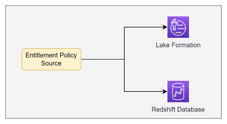
To solve this problem, we needed to build our own solution to convert the tag-based policies in Lake Formation into grants and revokes in the resource-based entitlements in Amazon Redshift.
Solution overview
To solve this mismatch, we wanted to synchronize our Lake Formation tag ontology and classifications to the Amazon Redshift permission model. To do this, we map Lake Formation tags and grants to Amazon Redshift grants with the following steps:
- Map all the resources (databases, schemas, tables, and more) in Lake Formation that are tagged to their equivalent Amazon Redshift tables.
- Translate each policy in Lake Formation on a tag expression to a set of Amazon Redshift table grants and revokes.
The net result is that when there is a tag or policy change in Lake Formation, a corresponding set of grants or revokes are made to the equivalent Amazon Redshift tables to keep our entitlements in sync.
Map all tagged resources in Lake Formation to Amazon Redshift equivalents
The tag-based access control of Lake Formation allowed us to apply multiple tags on a single resource (database and table) in the AWS Glue Data Catalog. If visualized in a mapping form, the resource tagging can be displayed as how multiple tags on a single table would be flattened into individual entitlements on Amazon Redshift tables.
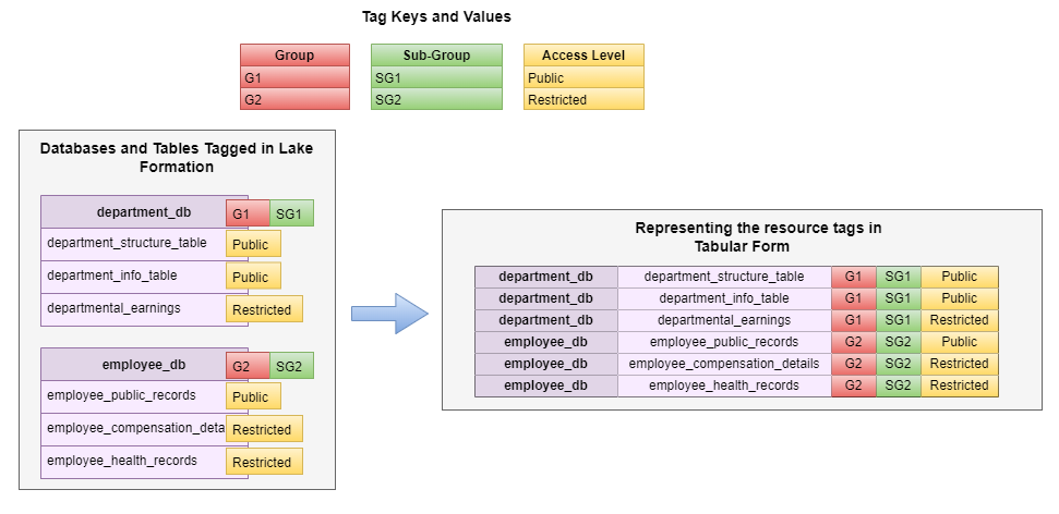
Translate tags to Amazon Redshift grants and revokes
To enable the migration of the tag-based policy enforced in Lake Formation, the permissions can be converted into simple grants and revokes that can be done on a per-group level.
There are two fundamental parts to a tag policy: the principal\_id and the tag expression (for example, “Acess Level” = “Public”). Assuming that we have an Amazon Redshift database group for each principal\_id, then the resources that represent the tag expression can be permissioned accordingly. We plan on migrating from database groups to database roles in a future implementation.
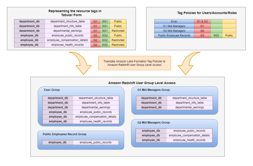
The solution implementation
The implementation of this solution led us to develop two components:
- The mapper service
- The Amazon Redshift data configuration
The mapper service can be thought of as a translation service. As the name suggests, it has the core business logic to map the tag and policy information into resource-based grants and revokes in Amazon Redshift. It needs to mimic the behavior of Lake Formation when handling the tag policy translation.
To do this translation, the mapper needs to understand and store the metadata at two levels:
- Understanding what resource in Amazon Redshift is to be tagged with what value
- Tracking the grants and revokes already performed so they can be updated with changes in the policy
To do this, we created a config schema in our Amazon Redshift cluster, which currently stores all the configurations.
As part of our implementation, we store the mapped (translated) information in Amazon Redshift. This allows us to incrementally update table grants as Lake Formation tags or policies changed. The following diagram illustrates this schema.

Business impact and value
The solution we put together has created key business impacts and values out of the current implementation and allows us greater flexibility in the future.
It allows us to get the data to our users faster with the tag policies applied in Lake Formation and translated directly to permissions in Amazon Redshift with immediate effect. It also allows us to have consistency in permissions applied in both Lake Formation and Amazon Redshift, based on the effective permissions derived from tag policies. And all this happens via a single source that grants and revokes permissions across the board, instead of managing them separately.
If we translate this into the business impact and business value that we generate, the solution improves the time to market of our data, but at the same time provides consistent entitlements across the business-driven categories that we define as tags.
The solution also opens up solutions to add more impact as our product scales both horizontally and vertically. There are potential solutions we could implement in terms of automation, users self-servicing their permissions, auditing, dashboards, and more. As our business scales, we expect to take advantage of these capabilities.
Conclusion
In this post, we shared how Morningstar utilized tag-based access control in our data lake with Lake Formation and enabled similar controls in Amazon Redshift. We developed two components that handle mapping of the tag-based access controls to Amazon Redshift permissions. This solution has improved the time to market for our data and provides consistent entitlements across different business-driven categories.
If you have any questions or comments, please leave them in the comments section.
About the Authors
 Ashish Prabhu is a Senior Manager of Software Engineering in Morningstar, Inc. He focuses on the solutioning and delivering the different aspects of Data Lake and Data Warehouse for Morningstar’s Enterprise Data and Platform Team. In his spare time he enjoys playing basketball, painting and spending time with his family.
 Stephen Johnston is a Distinguished Software Architect at Morningstar, Inc. His focus is on data lake and data warehousing technologies for Morningstar’s Enterprise Data Platform team.
 Colin Ingarfield is a Lead Software Engineer at Morningstar, Inc. Based in Austin, Colin focuses on access control and data entitlements on Morningstar’s growing Data Lake platform.
 Don Drake is a Senior Analytics Specialist Solutions Architect at AWS. Based in Chicago, Don helps Financial Services customers migrate workloads to AWS.
Amazon OpenSearch Service is used for a broad set of use cases like real-time application monitoring, log analytics, and website search at scale. As your domain ages and you add additional consumers, you need to reevaluate and change the domain’s configuration to handle additional storage and compute needs. You want to minimize downtime and performance impact as you make these changes.
Customers have been seeking guidance on best practices and patterns for changing index settings without an index maintenance window or affecting overall performance of the OpenSearch Service domain. This is part one of a two-part series, in which we show how to make settings changes to OpenSearch Service indexes with little to no downtime while supporting active producers and consumers of the data.
Indexes in OpenSearch Service
In OpenSearch Service, data must be indexed before it can be queried. Indexing is the method by which search engines organize data for fast retrieval. The resulting structure is called, fittingly, an index. All operations performed on an index are done via index APIs. Also, each index contains index mappings, which define field names and data types in the index. Data producers can add new fields with data types to an index. Index mappings can’t change throughout the index lifecycle.
OpenSearch Service indexes have two types of settings that periodically need adjustments as the profile of your workload changes:
- Dynamic – Settings that can be changed on the index at any time
- Static – Settings that can only be defined at the index creation time and can’t be changed throughout the index lifecycle
Dynamic index settings can be changed at any time using the update settings API. While the OpenSearch Service domain is performing instructed operations on dynamic index settings, the index doesn’t require a downtime. Changes to most dynamic index settings won’t trigger background tasks that affect the overall utilization of domain resources; however, some settings such as increasing the number of replicas via index.number\_of\_replicas or index.auto\_expand\_replicas, and depending on the domain’s configuration, can cause a temporary increase in resource utilization while the domain adds replicas. We recommend maintaining at least one replica for redundancy reasons, and multiple replicas for high query throughput use cases.
Static index settings such as mapping and shard count are defined at index creation time and can’t be changed throughout the index lifecycle. In this post, we focus on patterns and best practices for working with static index settings, such as changing shard count and patterns for updating index mappings.
All operations and procedures that we cover in this post are issued directly to the OpenSearch REST API or via the Dev Tools in OpenSearch Dashboards.
As with any use case, there is a spectrum of solutions and constraints to be considered. We start with a few simple foundational patterns and build on them, accounting for use cases with more operational constraints and working with large datasets.
Solution overview
OpenSearch Service has a default sharding strategy of 5:1, where each index is divided into five primary shards. Within each index, each primary shard also has its own replica. OpenSearch Service automatically assigns primary shards and replica shards to separate data nodes.
It’s not possible to increase the primary shard number of an existing index, meaning an index must be recreated if you want to increase the primary shard count.
The \_reindex operation is ideal for creating destination indexes with updated shards and mapping settings. The \_reindex operation is resource intensive. We recommend disabling replicas in your destination index by setting number\_of\_replicas to 0 and re-enable replicas when the reindex process is complete. If you have your data in a second, durable store, the simplest thing to do is pause updates and reindex from the source. But that’s not always possible. In this post, we share several patterns that enable you to update even static index settings like shard count.
One the major advantages of using the \_reindex operation is that it doesn’t require placing the source index in a read-only mode (data producers may continue to write the data while reindexing is in progress). Also, the \_reindex operation enables reprocessing, transformation, and reindexing a subset of documents and even selectively combining documents from multiple indexes. With the \_reindex operation, you can copy all or a subset of documents that you select through a query to another index. In its most basic form, the \_reindex operation requires you to specify a source and a destination index and configuration parameters.
The following are the some of the use cases supported by the reindex API:
- Reindexing all documents
- Reindexing from a remote cluster when transferring data between clusters
- Reindexing a subset of documents that match a search query
- Combining one or more indexes
- Transforming documents during reindexing
To increase the shard count, you create a new index, set number\_of\_shards to your desired primary shard count, set number\_of\_replicas to 0, update the new index mapping based on your requirement, and run the reindex API operation. After the \_reindex operation is complete, we recommend updating number\_of\_replicas in the destination index settings to achieve your desired level of replica shards.
In the following sections, we provide a walkthrough of the reindex API operation. Note that the patterns and procedures presented in this post have been validated on Amazon OpenSearch Service version 1.3.
Prerequisites
The source of the documents must be stored in the index (the “\_source” setting at the index mappings level must be set to “enabled”:true, which is the default). The \_reindex operation can’t be used without source documents.
Create the destination index with your desired mapping (field or data type). For demonstration purposes, our source index has a field ratings defined as long, and we want the same field to use the float data type in the destination index:
Ensure that you have sufficient disk space on each hot tier data node to house the new index primary shards and, depending on your configuration, replica shards. If disk space is insufficient, perform an update operation on the OpenSearch Service domain to add the required storage capacity. Depending on storage requirements, you may need to migrate the OpenSearch Service domain to a different instance type, because nodes have constraints on the EBS volume size that can be mounted to each instance type. Issue the following operation to validate available disk space:
The following screenshot shows the output.

Check the disk.avail metric for hot storage tier nodes to validate your available disk space.
Use the reindex API operation
The \_reindex operation snapshots the index at the beginning of its run and performs processing on a snapshot to minimize impact on the source index. The source index can still be used for querying and processing the data. Although the \_reindex operation can run both synchronously and asynchronously, we recommend using an asynchronous run. You can monitor the progress of the \_reindex operation, cancel its run, or throttle its run using the \_task, \_cancel, and \_rethrottle operations, respectively.
Because the \_reindex operation doesn’t require the source index placed in a read-only mode, query and index update operations are free to continue.
Use the reindex API with the following command:
The source indexes as part of the \_reindex API operation can be supplemented with a query for reindexing a subset of documents and storing them in the destination index. Progress of the re-indexing operation can be monitored via tasks API operation:
Note that the \_reindex operation can be throttled via a \_rethrottle API or settings passed as a parameter. You can cancel the task with the \_cancel operation:
The following screenshot shows the output of the \_reindex operation for reindexing from source\_index\_name to destination\_index\_name.

When the operation is complete, both consumers and producers of the source indexes or aliases need to re-point to the destination index and the same \_reindex operation needs to run again to catch up on any create, update, or delete operations performed on the source indexes while the initial \_reindex operation was running. This step is required because the \_reindex operation is running on a snapshot of the index. At this time, the \_reindex operation needs to run with “op\_type”:”create” to realign missing and out-of-version documents. See the following API command:
After the operation is complete and data integrity in the destination index is confirmed, you can delete the source index to reclaim disk space.
Increase index shard count using the split index API
The split index API and shrink index API cover a large array of use cases and present with low resource utilization in the domain. However, these APIs require closing the index for write operations and don’t address use cases that require changes to the mapping settings.
In OpenSearch Service, the number\_of\_shards index setting is immutable and defined at the time when the index is created. However, although this setting is immutable, there are several patterns to increase or decrease index shard count without needing to explicitly reindex the data. You can alternatively use the split index API to increase index shard count in the environments that can suspend write operations. The split index API provides a simplified way of creating a new index with a different shard setting and without reindexing your data. The split index API operation creates a new index based off of a read-only index with a desired number of primary shards.
In OpenSearch Service, an index alias is a virtual index name that can point to one or more indexes. Referencing to indexes using aliases in your applications allows you to avoid index name changes. Index aliases are used to point consumers and producers to a new index after the split index API operation is complete.
Although the majority of use cases focus on increasing a number of shards on an existing index due to data growth, there are also instances where you need to reduce the number of shards on an existing index. Such cases occasionally happen when an actual index size is less than what was anticipated when the index was created, and you want to align with a shard strategy for operational best practices for OpenSearch Service. In cases where you need to reduce a number of shards on an index, you can use the shrink index API to achieve this task.
Conclusion
In this post, we reviewed best practices when reindexing data for making changes in OpenSearch Service static index settings and mappings that require little or no index downtime. We also covered use of the split index and shrink index APIs for changing the primary index shard count for use cases where the index can be placed in a read-only state.
In our next post, we’ll explore patterns for remote indexing to alleviate load and resource utilization on the source OpenSearch Service domain.
About the Authors
 Mikhail Vaynshteyn is a Solutions Architect with Amazon Web Services. Mikhail works with healthcare and life sciences customers to build solutions that help improve patients’ outcomes. Mikhail specializes in data analytics services.
 Sukhomoy Basak is a Solutions Architect at Amazon Web Services, with a passion for data and analytics solutions. Sukhomoy works with enterprise customers to help them architect, build, and scale applications to achieve their business outcomes.
Amazon Redshift is a massively parallel processing (MPP), fully managed petabyte-scale data warehouse that makes it simple and cost-effective to analyze all your data using existing business intelligence tools.
When businesses are modernizing their data warehousing solutions to Amazon Redshift, implementing additional data protection mechanisms for sensitive data, such as personally identifiable information (PII) or protected health information (PHI), is a common requirement, especially for those in highly regulated industries with strict data security and privacy mandates. Amazon Redshift provides role-based access control, row-level security, column-level security, and dynamic data masking, along with other database security features to enable organizations to enforce fine-grained data security.
Security-sensitive applications often require column-level (or field-level) encryption to enforce fine-grained protection of sensitive data on top of the default server-side encryption (namely data encryption at rest). In other words, sensitive data should be always encrypted on disk and remain encrypted in memory, until users with proper permissions request to decrypt the data. Column-level encryption provides an additional layer of security to protect your sensitive data throughout system processing so that only certain users or applications can access it. This encryption ensures that only authorized principals that need the data, and have the required credentials to decrypt it, are able to do so.
In this post, we demonstrate how you can implement your own column-level encryption mechanism in Amazon Redshift using AWS Glue to encrypt sensitive data before loading data into Amazon Redshift, and using AWS Lambda as a user-defined function (UDF) in Amazon Redshift to decrypt the data using standard SQL statements. Lambda UDFs can be written in any of the programming languages supported by Lambda, such as Java, Go, PowerShell, Node.js, C#, Python, Ruby, or a custom runtime. You can use Lambda UDFs in any SQL statement such as SELECT, UPDATE, INSERT, or DELETE, and in any clause of the SQL statements where scalar functions are allowed.
Solution overview
The following diagram describes the solution architecture.

To illustrate how to set up this architecture, we walk you through the following steps:
- We upload a sample data file containing synthetic PII data to an Amazon Simple Storage Service (Amazon S3) bucket.
- A sample 256-bit data encryption key is generated and securely stored using AWS Secrets Manager.
- An AWS Glue job reads the data file from the S3 bucket, retrieves the data encryption key from Secrets Manager, performs data encryption for the PII columns, and loads the processed dataset into an Amazon Redshift table.
- We create a Lambda function to reference the same data encryption key from Secrets Manager, and implement data decryption logic for the received payload data.
- The Lambda function is registered as a Lambda UDF with a proper AWS Identity and Access Management (IAM) role that the Amazon Redshift cluster is authorized to assume.
- We can validate the data decryption functionality by issuing sample queries using Amazon Redshift Query Editor v2.0. You may optionally choose to test it with your own SQL client or business intelligence tools.
Prerequisites
To deploy the solution, make sure to complete the following prerequisites:
- Have an AWS account. For this post, you configure the required AWS resources using AWS CloudFormation in the
us-east-2Region. - Have an IAM user with permissions to manage AWS resources including Amazon S3, AWS Glue, Amazon Redshift, Secrets Manager, Lambda, and AWS Cloud9.
Deploy the solution using AWS CloudFormation
Provision the required AWS resources using a CloudFormation template by completing the following steps:
- Sign in to your AWS account.
- Choose Launch Stack:
- Navigate to an AWS Region (for example,
us-east-2). - For Stack name, enter a name for the stack or leave as default (
aws-blog-redshift-column-level-encryption). - For RedshiftMasterUsername, enter a user name for the admin user account of the Amazon Redshift cluster or leave as default (
master). - For RedshiftMasterUserPassword, enter a strong password for the admin user account of the Amazon Redshift cluster.
- Select I acknowledge that AWS CloudFormation might create IAM resources.
- Choose Create stack.

The CloudFormation stack creation process takes around 5–10 minutes to complete.
- When the stack creation is complete, on the stack Outputs tab, record the values of the following:
AWSCloud9IDEAmazonS3BucketForDataUploadIAMRoleForRedshiftLambdaUDFLambdaFunctionName

Upload the sample data file to Amazon S3
To test the column-level encryption capability, you can download the sample synthetic data generated by Mockaroo. The sample dataset contains synthetic PII and sensitive fields such as phone number, email address, and credit card number. In this post, we demonstrate how to encrypt the credit card number field, but you can apply the same method to other PII fields according to your own requirements.

An AWS Cloud9 instance is provisioned for you during the CloudFormation stack setup. You may access the instance from the AWS Cloud9 console, or by visiting the URL obtained from the CloudFormation stack output with the key AWSCloud9IDE.

On the AWS Cloud9 terminal, copy the sample dataset to your S3 bucket by running the following command:

Generate a secret and secure it using Secrets Manager
We generate a 256-bit secret to be used as the data encryption key. Complete the following steps:
- Create a new file in the AWS Cloud9 environment.

- Enter the following code snippet. We use the cryptography package to create a secret, and use the AWS SDK for Python (Boto3) to securely store the secret value with Secrets Manager:
- Save the file with the file name
generate\_secret.py(or any desired name ending with.py).

- Install the required packages by running the following
pip installcommand in the terminal: - Run the Python script via the following command to generate the secret:

Create a target table in Amazon Redshift
A single-node Amazon Redshift cluster is provisioned for you during the CloudFormation stack setup. To create the target table for storing the dataset with encrypted PII columns, complete the following steps:
- On the Amazon Redshift console, navigate to the list of provisioned clusters, and choose your cluster.
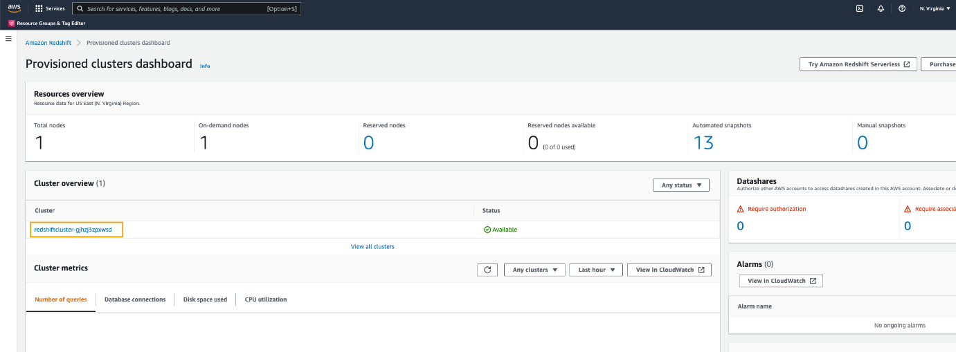
- To connect to the cluster, on the Query data drop-down menu, choose Query in query editor v2.

- If this is the first time you’re using the Amazon Redshift Query Editor V2, accept the default setting by choosing Configure account.

- To connect to the cluster, choose the cluster name.
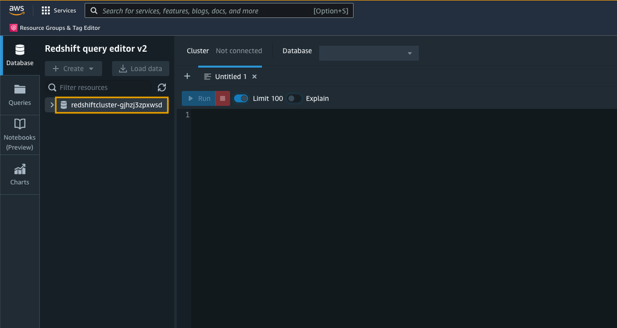
- For Database, enter
demodb. - For User name, enter
master. - For Password, enter your password.
You may need to change the user name and password according to your CloudFormation settings.
- Choose Create connection.
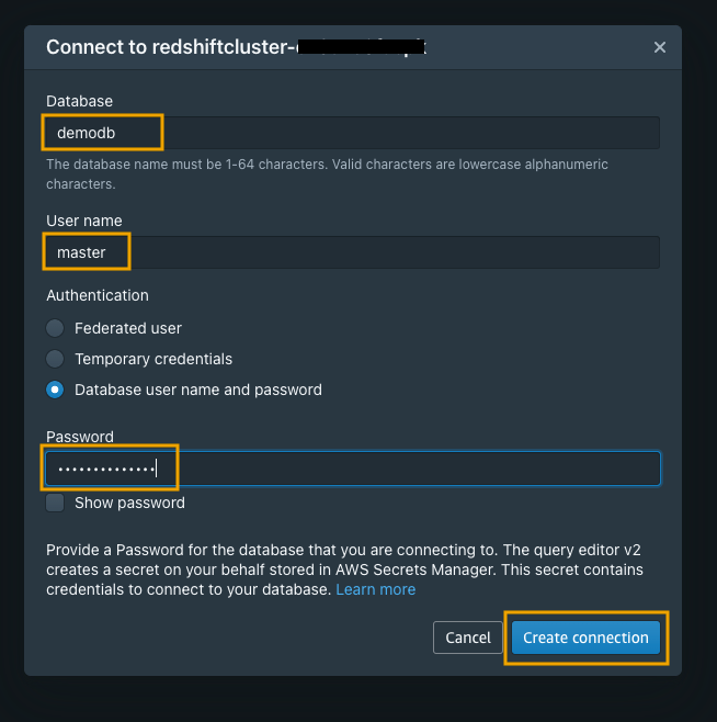
- In the query editor, run the following DDL command to create a table named
pii\_table:
We recommend using the smallest possible column size as a best practice, and you may need to modify these table definitions per your specific use case. Creating columns much larger than necessary will have an impact on the size of data tables and affect query performance.

Create the source and destination Data Catalog tables in AWS Glue
The CloudFormation stack provisioned two AWS Glue data crawlers: one for the Amazon S3 data source and one for the Amazon Redshift data source. To run the crawlers, complete the following steps:
- On the AWS Glue console, choose Crawlers in the navigation pane.

- Select the crawler named
glue-s3-crawler, then choose Run crawler to trigger the crawler job.

- Select the crawler named
glue-redshift-crawler, then choose Run crawler.

When the crawlers are complete, navigate to the Tables page to verify your results. You should see two tables registered under the demodb database.

Author an AWS Glue ETL job to perform data encryption
An AWS Glue job is provisioned for you as part of the CloudFormation stack setup, but the extract, transform, and load (ETL) script has not been created. We create and upload the ETL script to the /glue-script folder under the provisioned S3 bucket in order to run the AWS Glue job.
- Return to your AWS Cloud9 environment either via the AWS Cloud9 console, or by visiting the URL obtained from the CloudFormation stack output with the key
AWSCloud9IDE.
We use the Miscreant package for implementing a deterministic encryption using the AES-SIV encryption algorithm, which means that for any given plain text value, the generated encrypted value will be always the same. The benefit of using this encryption approach is to allow for point lookups, equality joins, grouping, and indexing on encrypted columns. However, you should also be aware of the potential security implication when applying deterministic encryption to low-cardinality data, such as gender, boolean values, and status flags.
- Create a new file in the AWS Cloud9 environment and enter the following code snippet:
- Save the script with the file name
pii-data-encryption.py.
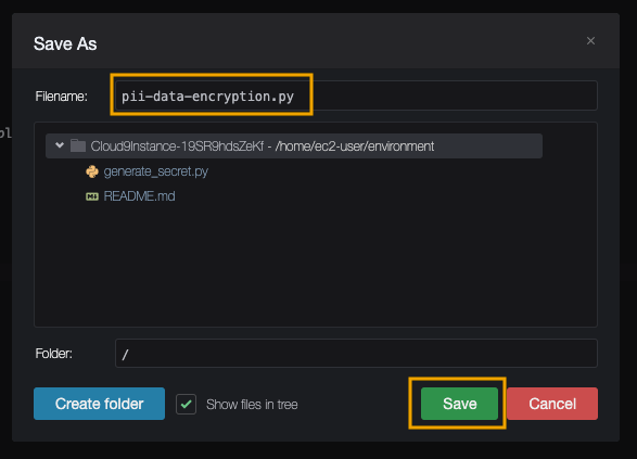
- Copy the script to the desired S3 bucket location by running the following command:

- To verify the script is uploaded successfully, navigate to the Jobs page on the AWS Glue console.You should be able to find a job named
pii-data-encryption-job.

- Choose Run to trigger the AWS Glue job.It will first read the source data from the S3 bucket registered in the AWS Glue Data Catalog, then apply column mappings to transform data into the expected data types, followed by performing PII fields encryption, and finally loading the encrypted data into the target Redshift table. The whole process should be completed within 5 minutes for this sample dataset.
 You can switch to the Runs tab to monitor the job status.

Configure a Lambda function to perform data decryption
A Lambda function with the data decryption logic is deployed for you during the CloudFormation stack setup. You can find the function on the Lambda console.

The following is the Python code used in the Lambda function:
If you want to deploy the Lambda function on your own, make sure to include the Miscreant package in your deployment package.
Register a Lambda UDF in Amazon Redshift
You can create Lambda UDFs that use custom functions defined in Lambda as part of your SQL queries. Lambda UDFs are managed in Lambda, and you can control the access privileges to invoke these UDFs in Amazon Redshift.
- Navigate back to the Amazon Redshift Query Editor V2 to register the Lambda UDF.
- Use the
CREATE EXTERNAL FUNCTIONcommand and provide an IAM role that the Amazon Redshift cluster is authorized to assume and make calls to Lambda:
You can find the Lambda name and Amazon Redshift IAM role on the CloudFormation stack Outputs tab:
LambdaFunctionNameIAMRoleForRedshiftLambdaUDF

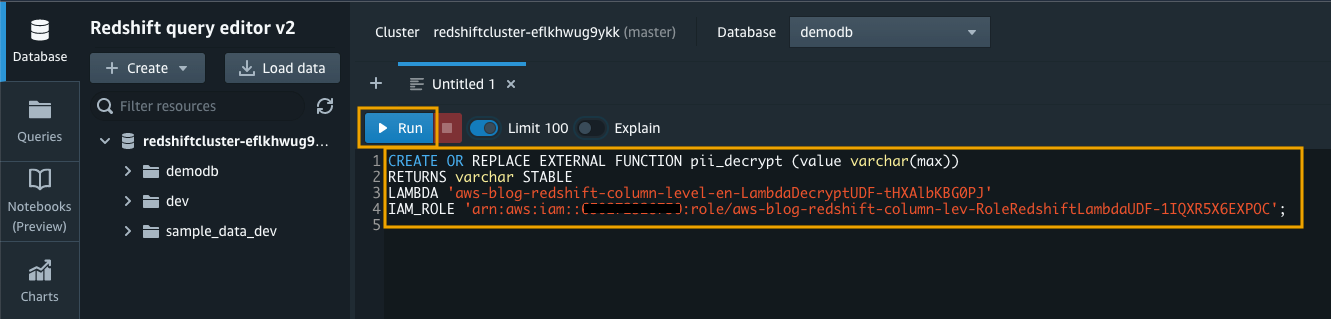
Validate the column-level encryption functionality in Amazon Redshift
By default, permission to run new Lambda UDFs is granted to PUBLIC. To restrict usage of the newly created UDF, revoke the permission from PUBLIC and then grant the privilege to specific users or groups. To learn more about Lambda UDF security and privileges, see Managing Lambda UDF security and privileges.
You must be a superuser or have the sys:secadmin role to run the following SQL statements:
First, we run a SELECT statement to verify that our highly sensitive data field, in this case the registered\_credit\_card column, is now encrypted in the Amazon Redshift table:

For regular database users who have not been granted the permission to use the Lambda UDF, they will see a permission denied error when they try to use the pii\_decrypt() function:

For privileged database users who have been granted the permission to use the Lambda UDF for decrypting the data, they can issue a SQL statement using the pii\_decrypt() function:
The original registered\_credit\_card values can be successfully retrieved, as shown in the decrypted\_credit\_card column.
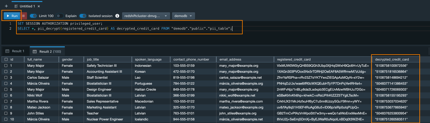
Cleaning up
To avoid incurring future charges, make sure to clean up all the AWS resources that you created as part of this post.
You can delete the CloudFormation stack on the AWS CloudFormation console or via the AWS Command Line Interface (AWS CLI). The default stack name is aws-blog-redshift-column-level-encryption.
Conclusion
In this post, we demonstrated how to implement a custom column-level encryption solution for Amazon Redshift, which provides an additional layer of protection for sensitive data stored on the cloud data warehouse. The CloudFormation template gives you an easy way to set up the data pipeline, which you can further customize for your specific business scenarios. You can also modify the AWS Glue ETL code to encrypt multiple data fields at the same time, and to use different data encryption keys for different columns for enhanced data security. With this solution, you can limit the occasions where human actors can access sensitive data stored in plain text on the data warehouse.
You can learn more about this solution and the source code by visiting the GitHub repository. To learn more about how to use Amazon Redshift UDFs to solve different business problems, refer to Example uses of user-defined functions (UDFs) and Amazon Redshift UDFs.
About the Author
 Aaron Chong is an Enterprise Solutions Architect at Amazon Web Services Hong Kong. He specializes in the data analytics domain, and works with a wide range of customers to build big data analytics platforms, modernize data engineering practices, and advocate AI/ML democratization.
Showpad aligns sales and marketing teams around impactful content and powerful training, helping sellers engage with buyers and generate the insights needed to continuously improve conversion rates. In 2021, Showpad set forth the vision to use the power of data to unlock innovations and drive business decisions across its organization. Showpad’s legacy solution was fragmented and expensive, with different tools providing conflicting insights and lengthening time to insight. The company decided to use AWS to unify its business intelligence (BI) and reporting strategy for both internal organization-wide use cases and in-product embedded analytics targeted at its customers.
Showpad built new customer-facing embedded dashboards within Showpad eOSTM and migrated its legacy dashboards to Amazon QuickSight, a unified BI service providing modern interactive dashboards, natural language querying, paginated reports, machine learning (ML) insights, and embedded analytics at scale.
In this post, we share how Showpad used QuickSight to streamline data and insights access across teams and customers. Showpad migrated over 70 dashboards with over 1,000 visuals. They have rolled out the solution to all its 600 employees, increased dashboard development activity by three times, and reduced dashboard turnaround time from months to weeks. Showpad also launched dashboards and reports to over 1,300 customers worldwide, providing access to tens of thousands of users across all its customers.
Streamlining data-driven decisions by defragmenting the data and reporting architecture
Founded in 2011, dual headquartered in Belgium and Chicago and with offices around the world, Showpad provides a single destination for sales representatives to access all sales content and information, along with coaching and training tools to create informed, upskilled, and trusted buying teams. The platform also provides analytics and insights to support successful information sharing and fuel continuous improvement. In 2021, Showpad decided to take the next step in its data evolution and set forth the vision to power innovation, product decisions, and customer engagement using data-driven insights. This required Showpad to accelerate its data maturity as a company by mindfully using data and technology holistically to help its customers.
But the company’s legacy BI solution and data were fragmented across multiple tools, some with proprietary logic. “Each of these tools were getting data from a different place, and that’s where it gets difficult,” says Jeroen Minnaert, head of data at Showpad. “If each tool tells a different story because it has different data, we won’t have alignment within the business on what this data means.” Showpad also struggled with data quality issues in terms of consistency, ownership, and insufficient data access across its targeted user base due to a complex BI access process, licensing challenges, and insufficient education.
Showpad wanted to unify all the data into a single unified interface through a data lake, democratize that data through a BI solution such that autonomous teams across the company could effectively use data, and drive and unlock innovation in the company through advanced insights data, artificial intelligence, and ML. The company already used AWS in other aspects of its business and found that QuickSight would not only meet all its BI and reporting needs with seamless integrations into the AWS stack, but also bring with it several unique benefits unlike incumbents and other tools evaluated. “We chose QuickSight because of its embedded analytic capabilities, serverless architecture, and consumption-based pricing,” says Minnaert. “Using QuickSight to launch interactive dashboards and reporting for our customers, along with the ability for our customer success teams to create or alter dashboard prototypes on our internal-facing QuickSight instance and then promote those dashboards to customers through the product, was a very compelling use case.”
QuickSight would help local data stewards, who weren’t technical but knew the use cases intimately, to create their own dashboards and prototype them with their customers before promoting them through the product. “The serverless model was also compelling because we did not have to pay for server instances nor license fees per reader. With QuickSight, we pay for usage. This makes it easy for us to provide access to everyone by default. This is a key pillar in our ability to democratize data,” says Minnaert.
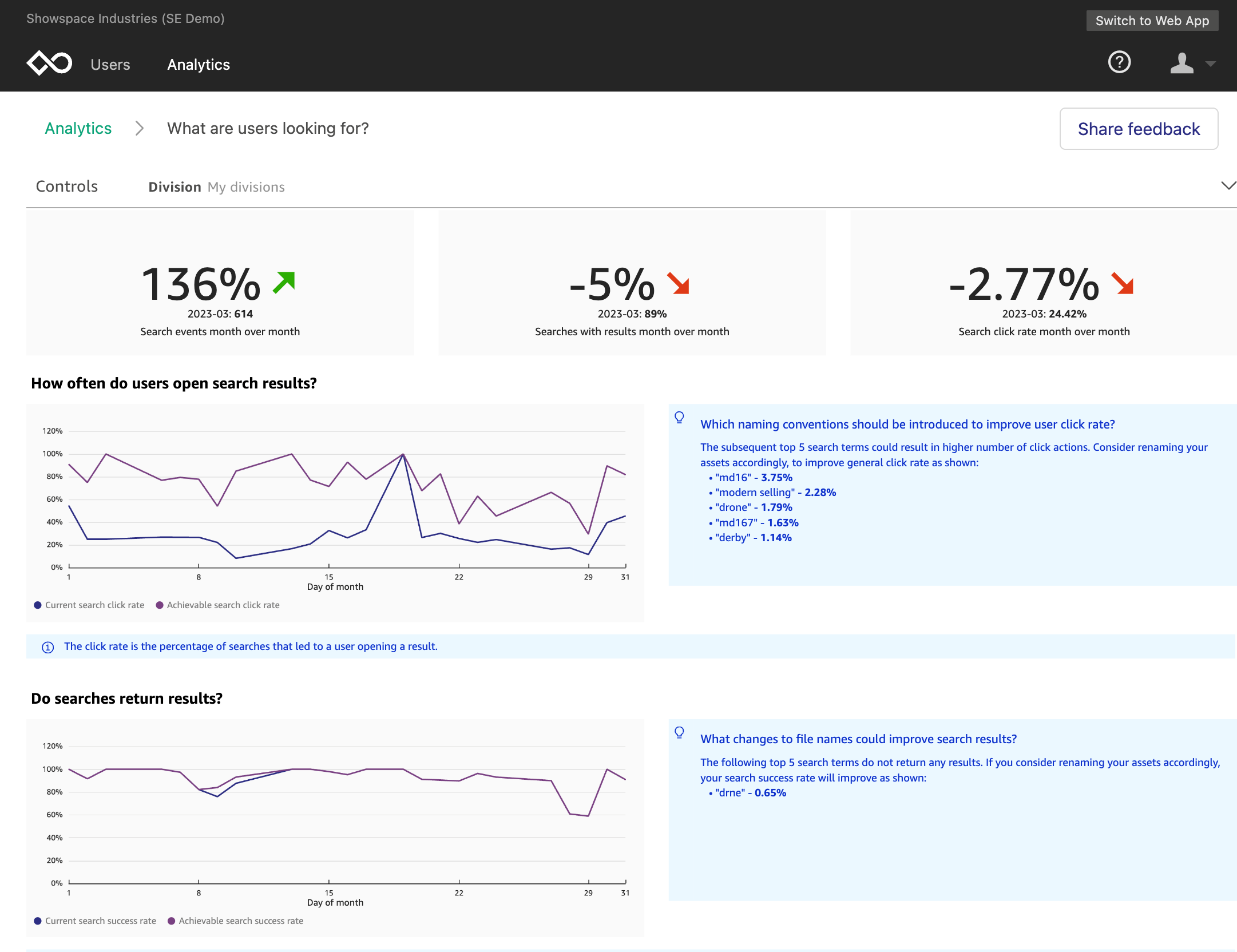
Architecting a portable data layer and migrating to QuickSight to accelerate time to value
After choosing QuickSight as its solution in November 2021, Showpad took on two streams of development: migrating internal organization-wide BI reporting and building in-product reporting using embedded analytics. Showpad worked closely alongside the QuickSight team to have a smooth rollout. The company involved members of the QuickSight team in its internal communications and set up meetings every 2 weeks to resolve difficult issues quickly.
On the internal reporting front, the data team took a “working backwards” approach to make sure it had the right approach before going all in with all existing dashboards. Showpad selected five difficult and complex dashboards and took 3 months to explore various possibilities using QuickSight. For example, the team determined that user log-in would be automated with single sign-on and Okta and built a plan for assets organization, asset promotion, and access controls. The company also used the opportunity to reimagine its data pipeline and architecture. A key architectural decision that Showpad took during this time was to create a portable data layer by decoupling the data transformation from visualization, ML, or ad hoc querying tools and centralizing its business logic. The portable data layer facilitated the creation of data products for varied use cases, made available within various tools based on the need of the consumer—be it a business analyst, data scientist, or business user.
After the solution approach was decided on and the foundation was built, the team wanted to scale. However, with 70 dashboards with over 1,000 visuals with varying levels of complexities, including proprietary logic unique to certain tools, and data from over 1,000 tables ingesting data from over 20 data sources, the team decided to take a measured approach to the migration. The entire data team of 20 people were “all on hands on deck” for the project.
First, Showpad created a landscape of all the dashboards, connecting data sources and dependencies before prioritizing the migration order. The company decided to start with dashboards with the fewest dependencies, like product and engineering dashboards that had a single data source, followed by revenue operations dashboards with a couple of data sources, and lastly with customer success and marketing dashboards that combined product and engineering and revenue operations data. After migration was complete, Showpad validated all the numbers and worked with business stakeholders for quality assurance. It launched the first set of dashboards in April 2022, followed by customer success and marketing dashboards in July 2022. As of January 2023, Showpad’s QuickSight instance includes over 2,433 datasets and 199 dashboards.
Showpad also achieves benefits for its customers by using QuickSight to deliver a wide variety of insights, including usage dashboards, industry comparisons, user comparison, group comparison, and revenue attribution. On the second workstream of in-product customer-facing reporting, Showpad released its first version of QuickSight reporting to customers in June 2022. “We went through user research, development, and beta tests in a span of 6 months, which was a fast turnaround and a big win for us,” says Minnaert. And Showpad aims to further accelerate the turnaround time to make a report and ship it to a customer.
With the foundational architecture now in place, shipping to a customer can happen in a few sprints, with most of the time spent on iterating and fine-tuning insights instead of engineering a scalable reporting solution. Showpad can also improve the insights it offers to customers. “Using QuickSight in our product makes it a powerful tool,” says Minnaert. “We can launch reporting for our customers so that they can look at and interpret data by themselves.” Showpad can then follow up with tailor-made reporting for each customer using the same data so that it tells a consistent story.
After a dashboard is agreed on, the dashboard can go through Showpad’s automated dashboard promotion process that can take an idea from development to production to a smile on a customer’s face in weeks, not months.
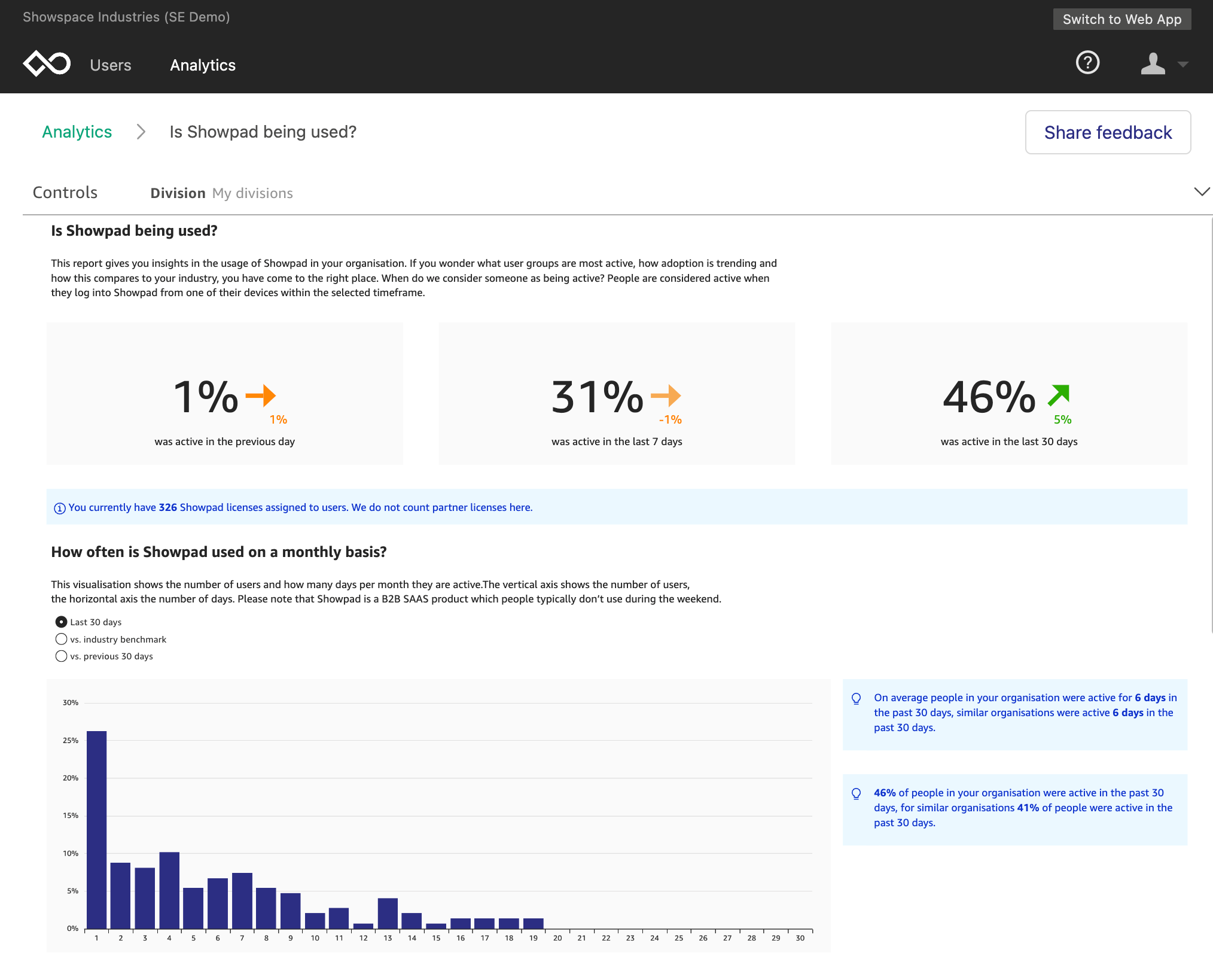
Unlocking innovation with self-service BI and rapid prototyping
By providing dashboard and report building to analysts and nontechnical users, Showpad drastically reduced overall turnaround time to build and deliver insights, down from months to weeks. Showpad also increased dashboard development activity by three times across the organization.
Showpad users can quickly prototype reports in a well-known environment—building reports using QuickSight, and then testing them with customers by helping customers understand how the reporting would look and function. “After we settle on reports or dashboards, it does not take much engineering effort to bring them to production,” says Minnaert. “We can make a lot of innovation happen by quickly prototyping and bringing validated prototypes to production.” Showpad’s users and customers also benefit from performance gains with 10 times increased speed when using SPICE (Super-fast, Parallel, In-memory Calculation Engine), which is the robust in-memory engine that QuickSight uses. It takes only seconds to load dashboards.
Because QuickSight is serverless and uses a session-based pricing model, Showpad expects to see cost savings. By paying per use, Showpad can easily provide access to all its users and customers without purchasing expensive per-reader licenses. Showpad also doesn’t need to pay for server instances or maintain infrastructure for BI. In addition, Showpad can deprecate custom reporting, infrastructure, and multiple tools with the new data architecture and QuickSight. “Much of our cost savings will come from being able to deprecate the custom reporting that we’ve made in the past,” says Minnaert. “The custom reporting used a lot of infrastructure that we no longer need to maintain.” Showpad expects to see a three times increase in projected return on investment in the upcoming year.
Showpad completed its internal BI migration to QuickSight by the end of 2022. Showpad also continues to expand the in-product reporting while continuing to optimize performance for the best customer experience. Showpad hopes to further reduce the time it takes to load a dashboard to under 1 second.
In conjunction with Showpad’s new portable data layer, QuickSight helps users of all types across its organization and customers self-serve data and insights rapidly. Everyone in Showpad gets access to data and insights the day they onboard with Showpad. To make self-service even easier, Showpad will soon launch embedded Amazon QuickSight Q so anyone can ask questions in natural language and receive accurate answers with relevant visualizations that help them gain insights from the data. By helping business users and experts rapidly prototype dashboards and reports in line with user and customer needs, Showpad uses the power of data to unlock innovation and drive growth across its organization. “QuickSight has become our go-to tool for any BI requirement at Showpad—both internal and external customer facing, especially when it comes to correlating data across departments and business units,” says Minnaert.
Get started with QuickSight
Migrating to QuickSight enabled Showpad to streamline data and insights access across teams and customers and reduced overall turnaround time to build and deliver insights from months to weeks.
Learn more about unleashing your organization’s ability to accelerate revenue growth with Showpad. To learn more about how QuickSight can help your business with dashboards, reports, and more, visit Amazon QuickSight.
About the Author
 Shruthi Panicker is a Senior Product Marketing Manager with Amazon QuickSight at AWS. As an engineer turned product marketer, Shruthi has spent over 15 years in the technology industry in various roles from software engineering, to solution architecting to product marketing. She is passionate about working at the intersection of technology and business to tell great product stories that help drive customer value.
Amazon QuickSight previously launched threshold alerts on KPIs and gauge charts. Now, QuickSight supports creating threshold alerts on tables and pivot tables—our most popular visual types. This allows readers and authors to track goals or key performance indicators (KPIs) and be notified via email when they are met. These alerts allow readers and authors to relax and rely on notifications for when their attention is needed. In this post, we share how to create threshold alerts on tables or pivot tables to track important metrics.
Background information
Threshold alerts are a QuickSight Enterprise Edition feature and available for dashboards consumed on the QuickSight website. Threshold alerts aren’t yet available in embedded QuickSight dashboards or on the mobile app.
Alerts are created based on the visual at that point in time and are not affected by potential future changes to the visual’s design. This means the visual can be changed or deleted and the alert continues to work as long as the data in the dataset remains valid. In addition, you can create multiple alerts off of one visual, and rename them as appropriate.
Finally, alerts respect RLS and CLS rules.
Set up an alert on a table or pivot table
Threshold alerts are configured for dashboards. On a dashboard, there are three different ways to create an alert on a table or pivot table.
First, you can create directly from a pivot table or table. You click directly on the cell you would like to create an alert on (if there is another action enabled, you may have to right-click to get this option to show). This needs to be on a numeric value (no dates or strings allow for creation of alerts). Then choose Create Alert to start creating the alert.
Let’s assume you want to track the profit coming from online purchases for auto-related merchandise being shipped first class. Choose the appropriate cell and then choose Create Alert.
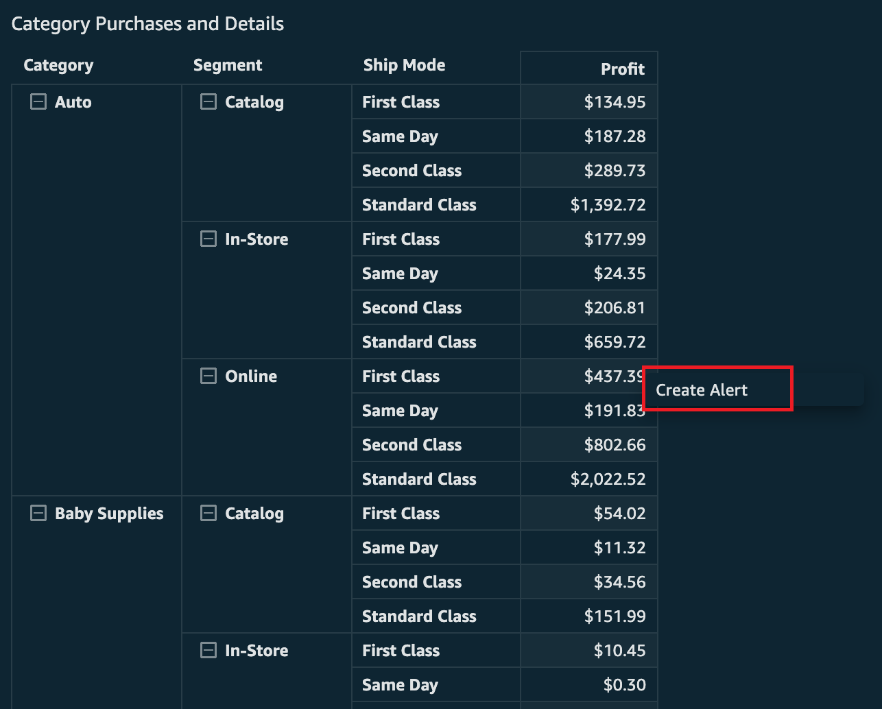
You’re presented with the creation pane for alerts. The only difference from KPIs or gauge visual alerts is that here you’ll find the other dimensions in the row that you’re creating the alert on. This will help you identify what value from the table you have selected, because there can be duplicates of the numeric values.
In the following screenshot, the value to track is profit, which currently is $437.39. This is the value that will be compared to the threshold you set. You will also see the dimensions being used to define this alert, which are taken from the row of the table. In this case, the Category is Auto, the Segement is Online, and the Ship Mode is First Class.

Now that you have checked that the value is correct, you can update the name of the alert that is automatically filled with the name of the visual it is created off of, set the condition (between Is above, Is below, and Is equal to), and pick the threshold value, notification frequency, and whether you want to be emailed when there is no data.
In the following example, the alert has been configured so that you will receive an email when the profit is above the threshold of $1,000. You’ve also left the notification frquency at Daily at most and haven’t requested to be emailed when there is no data.

If you have a date field, you also will see an option to control the date. This will automatically set the date field to be the most recent of whatever aggregation you’re looking at, such as hour, week, day, month. However, you could override to use the specific date applied to the value you have selected if you would prefer.
Below is an example where the data was aggregated based on the week and so Latest Week has been selected rather than the historical Week of Jan 4, 2015.

You can then choose Save if you’re happy with the alert and it will load the Manage alert pane.
The Create Alert button is also at the bottom of the pane. This is the second way you can start creating an alert off of a table or pivot table.
You can also get to this pane from the upper right alert button on the dashboard.

If you have no alerts, this will automatically drop you into the creation pane. There you will be asked to select a visual that supports alerts to begin creating an alert. If you already have alerts (as previously demonstrated), then all you need to do is choose Create Alert.
Then select a visual and choose Next.
You’re prompted to select a cell if you have picked a table or pivot table visual.
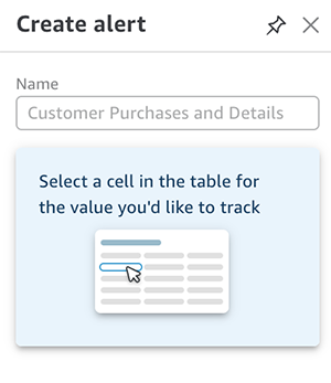
Then you repeat the same steps as creating off a cell within a table or pivot table.
Finally, you can start creating an alert from the bell icon on the pivot table or table. This is the third way to create an alert.
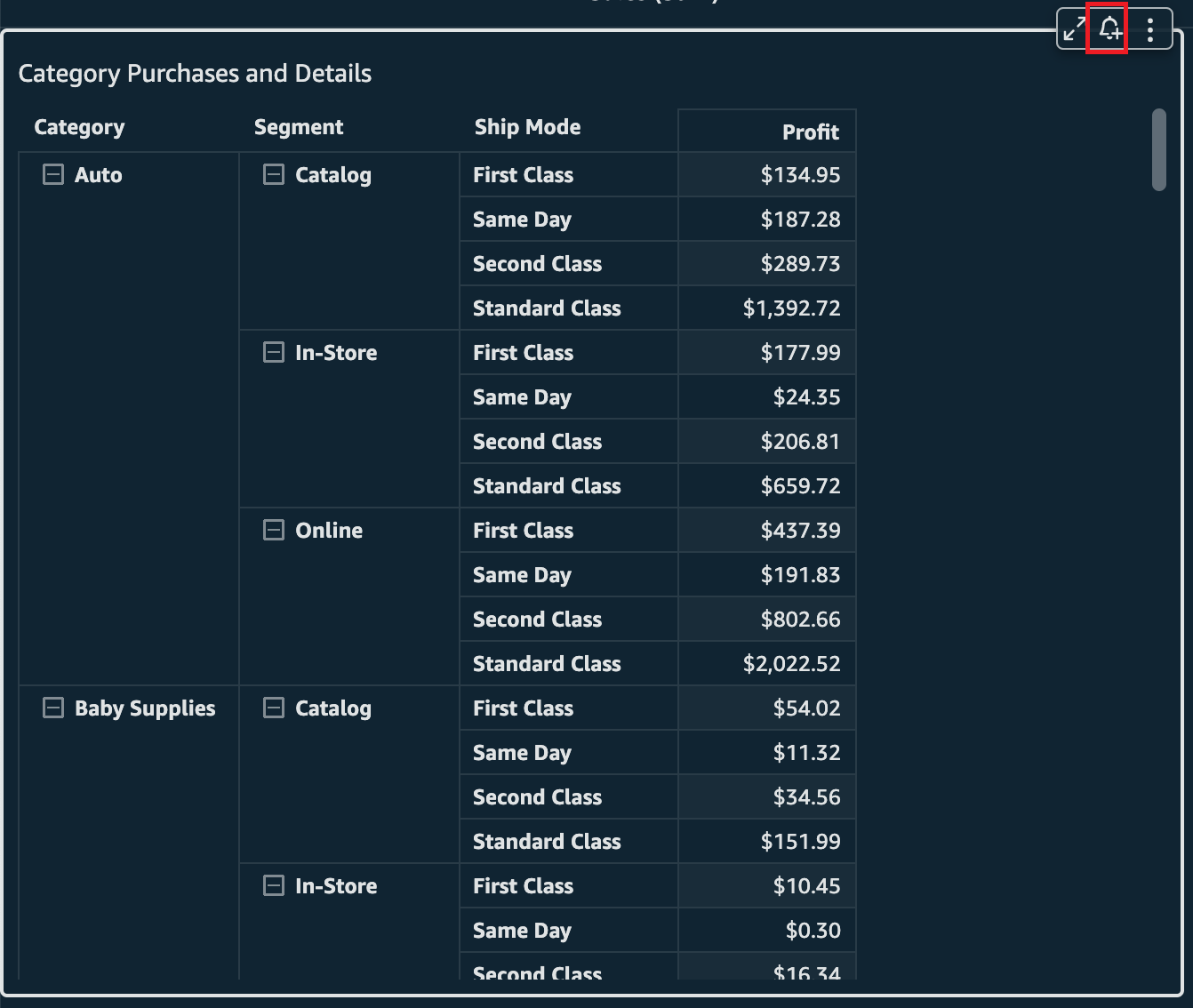
You’ll be prompted to select a cell from the table, and the creation pane appears.
After you choose the cell that you want to track, you start the creation process just like the first two examples.
Update and delete alerts
To update or delete an alert, you need to navigate back to the Manage alerts pane. You get there from the bell icon on the top right corner of the dashboard.
You can then choose the options menu (three dots) on the alert you want to manage. Three options appear: Edit alert, View history (to view recent times the alert has breached and notified you), and Delete.

Notifications
You’ll receive an email when your alert breaches the rule you set. The following is an example of what that looks like (the alert has been adjusted to be alerted if profit is over $100 and to be notified as frequently as possible).

The current profit breach is highlighted and the historical numbers are shown along with the date and time of the recorded breaches. You can also navigate to the dashboard by choosing View Dashboard.
Evaluate alerts
The evaluation schedule for threshold alerts is based on the dataset. For SPICE datasets, alert rules are checked against the data after a successful data refresh. With datasets querying your data sources directly, alerts are evaluated daily at a random time between 6:00 PM and 8:00 AM. This is based on the the timezone of the AWS Region your dataset was created in. Dataset owners can set up their own schedules for checking alerts and increase the frequency up to hourly (to learn more, refer to Working with threshold alerts in Amazon QuickSight).
Restrict alerts
The admin for the QuickSight account can restrict who has access to set threshold alerts through custom permissions. For more information, see the section Customizing user permissions in Embed multi-tenant analytics in applications with Amazon QuickSight.
Pricing
Threshold alerts are billed for each evaluation, and follow the familiar pricing used for anomaly detection, starting at $0.50 per 1,000 evaluations. For example, if you set up an alert on a SPICE dataset that refreshes daily, you have 30 evaluations of the alert rule in a month, which costs 30 * $0.5/1000 = $0.015 in a month. For more information, refer to Amazon QuickSight Pricing.
Conclusion
In this post, you learned how to create threshold alerts on tables and pivot tables within QuickSight dashboards so that you can track important metrics. For more information about how to create threshold alerts on KPIs or gauge charts, refer to Create threshold-based alerts in Amazon QuickSight. Additional information is available in the Amazon QuickSight User Guide.
About the Author
 Lillie Atkins is a Product Manager for Amazon QuickSight, Amazon Web Service’s cloud-native, fully managed BI service.
Tens of thousands of customers run business-critical workloads on Amazon Redshift, AWS’s fast, petabyte-scale cloud data warehouse delivering the best price-performance. With Amazon Redshift, you can query data across your data warehouse, operational data stores, and data lake using standard SQL. You can also integrate AWS services like Amazon EMR, Amazon Athena, Amazon SageMaker, AWS Glue, AWS Lake Formation, and Amazon Kinesis to take advantage of all of the analytic capabilities in the AWS Cloud.
Amazon Redshift RSQL is a native command-line client for interacting with Amazon Redshift clusters and databases. You can connect to an Amazon Redshift cluster, describe database objects, query data, and view query results in various output formats. You can use Amazon Redshift RSQL to replace existing extract, transform, load (ETL) and automation scripts, such as Teradata BTEQ scripts. You can wrap Amazon Redshift RSQL statements within a shell script to replicate existing functionality in the on-premise systems. Amazon Redshift RSQL is available for Linux, Windows, and macOS operating systems.
This post explains how you can create a generic configuration-driven orchestration framework using AWS Step Functions, Amazon Elastic Compute Cloud (Amazon EC2), AWS Lambda, Amazon DynamoDB, and AWS Systems Manager to orchestrate RSQL-based ETL workloads. If you’re migrating from legacy data warehouse workloads to Amazon Redshift, you can use this methodology to orchestrate your data warehousing workloads.
Solution overview
Customers migrating from legacy data warehouses to Amazon Redshift may have a significant investment in proprietary scripts like Basic Teradata Query (BTEQ) scripting for database automation, ETL, or other tasks. You can now use the AWS Schema Conversion Tool (AWS SCT) to automatically convert proprietary scripts like BTEQ scripts to Amazon Redshift RSQL scripts. The converted scripts run on Amazon Redshift with little to no changes. To learn about new options for database scripting, refer to Accelerate your data warehouse migration to Amazon Redshift – Part 4.
During such migrations, you may also want to modernize your current on-premises, third-party orchestration tools with a cloud-native framework to replicate and enhance your current orchestration capability. Orchestrating data warehouse workloads includes scheduling the jobs, checking if the pre-conditions have been met, running the business logic embedded within RSQL, monitoring the status of the jobs, and alerting if there are any failures.
This solution allows on-premises customers to migrate to a cloud-native orchestration framework that uses AWS serverless services such as Step Functions, Lambda, DynamoDB, and Systems Manager to run the Amazon Redshift RSQL jobs deployed on a persistent EC2 instance. You can also deploy the solution for greenfield implementations. In addition to meeting functional requirements, this solution also provides full auditing, logging, and monitoring of all ETL and ELT processes that are run.
To ensure high availability and resilience, you can use multiple EC2 instances that are a part of an auto scaling group along with Amazon Elastic File System (Amazon EFS) to deploy and run the RSQL jobs. When using auto scaling groups, you can install RSQL onto the EC2 instance as a part of the bootstrap script. You can also deploy the Amazon Redshift RSQL scripts onto the EC2 instance using AWS CodePipeline and AWS CodeDeploy. For more details, refer to Auto Scaling groups, the Amazon EFT User Guide, and Integrating CodeDeploy with Amazon EC2 Auto Scaling.
The following diagram illustrates the architecture of the orchestration framework.

The key components of the framework are as follows:
- Amazon EventBridge is used as the ETL workflow scheduler, and it triggers a Lambda function at a preset schedule.
- The function queries a DynamoDB table for the configuration associated to the RSQL job and queries the status of the job, run mode, and restart information for that job.
- After receiving the configuration, the function triggers a Step Functions state machine by passing the configuration details.
- Step Functions starts running different stages (like configuration iteration, run type check, and more) of the workflow.
- Step Functions uses the Systems Manager
SendCommandAPI to trigger the RSQL job and goes into a paused state withTaskToken. The RSQL scripts are persisted on an EC2 instance and are wrapped in a shell script. Systems Manager runs anAWS-RunShellScriptSSM document to run the RSQL job on the EC2 instance. - The RSQL job performs ETL and ELT operations on the Amazon Redshift cluster. When it’s complete, it returns a success/failure code and status message back to the calling shell script.
- The shell script calls a custom Python module with the success/failure code, status message, and the callwait
TaskTokenthat was received from Step Functions. The Python module logs the RSQL job status in the job audit DynamoDB audit table, and exports logs to the Amazon CloudWatch log group. - The Python module then performs a
SendTaskSuccessorSendTaskFailureAPI call based on the RSQL job run status. Based on the status of the RSQL job, Step Functions either resumes the flow or stops with failure. - Step Functions logs the workflow status (success or failure) in the DynamoDB workflow audit table.
Prerequisites
You should have the following prerequisites:
- An AWS account.
- The AWS Cloud Development Kit (AWS CDK) installed on the development environment. For more information, refer to Prerequisites.
- An Amazon Redshift cluster.
- Amazon Redshift database credentials stored in AWS Secrets Manager. For more information, refer to Storing database credentials in AWS Secrets Manager. After you create the secret, modify it to add the name of the Amazon Redshift database with the secret key
dbname. For instructions, refer to Modify an AWS Secrets Manager secret. - An Amazon Linux 2 EC2 instance with Amazon Redshift RSQL installed.
Deploy AWS CDK stacks
Complete the following steps to deploy your resources using the AWS CDK:
- Clone the GitHub repo:
- Update the following the environment parameters in
cdk.json(this file can be found in the infra directory):- ec2\_instance\_id – The EC2 instance ID on which RSQL jobs are deployed
- redshift\_secret\_id – The name of the Secrets Manager key that stores the Amazon Redshift database credentials
- rsql\_script\_path – The absolute directory path in the EC2 instance where the RSQL jobs are stored
- rsql\_log\_path – The absolute directory path in the EC2 instance used for storing the RSQL job logs
- rsql\_script\_wrapper – The absolute directory path of the RSQL wrapper script (rsql\_trigger.sh) on the EC2 instance.
The following is a sample
cdk.jsonfile after being populated with the parameters - Deploy the AWS CDK stack with the following code:
Let’s look at the resources the AWS CDK stack deploys in more detail.
CloudWatch log group
A CloudWatch log group (/ops/rsql-logs/) is created, which is used to store, monitor, and access log files from EC2 instances and other sources.
The log group is used to store the RSQL job run logs. For each RSQL script, all the stdout and stderr logs are stored as a log stream within this log group.
DynamoDB configuration table
The DynamoDB configuration table (rsql-blog-rsql-config-table) is the basic building block of this solution. All the RSQL jobs, restart information and run mode (sequential or parallel), and sequence in which the jobs are to be run are stored in this configuration table.
The table has the following structure:
- workflow\_id – The identifier for the RSQL-based ETL workflow.
- workflow\_description – The description for the RSQL-based ETL workflow.
- workflow\_stages – The sequence of stages within a workflow.
- execution\_type – The type of run for RSQL jobs (sequential or parallel).
- stage\_description – The description for the stage.
- scripts – The list of RSQL scripts to be run. The RSQL scripts must be placed in the location defined in a later step.
The following is an example of an entry in the configuration table. You can see the workflow\_id is blog\_test\_workflow and the description is Test Workflow for Blog.
It has three stages that are triggered in the following order: Schema & Table Creation Stage, Data Insertion Stage 1, and Data Insertion Stage 2. The stage Schema & Table Creation Stage has two RSQL jobs running sequentially, and Data Insertion Stage 1 and Data Insertion Stage 2 each have two jobs running in parallel.
DynamoDB audit tables
The audit tables store the run details for each RSQL job within the ETL workflow with a unique identifier for monitoring and reporting purposes. The reason why there are two audit tables is because one table stores the audit information at a RSQL job level and the other stores it at a workflow level.
The job audit table (rsql-blog-rsql-job-audit-table) has the following structure:
- job\_name – The name of the RSQL script
- workflow\_execution\_id – The run ID for the workflow
- execution\_start\_ts – The start timestamp for the RSQL job
- execution\_end\_ts – The end timestamp for the RSQL job
- execution\_status – The run status of the RSQL job (
Running, Completed, Failed) - instance\_id – The EC2 instance ID on which the RSQL job is run
- ssm\_command\_id – The Systems Manager command ID used to trigger the RSQL job
- workflow\_id – The
workflow\_idunder which the RSQL job is run
The workflow audit table (rsql-blog-rsql-workflow-audit-table) has the following structure:
- workflow\_execution\_id – The run ID for the workflow
- workflow\_id – The identifier for a particular workflow
- execution\_start\_ts – The start timestamp for the workflow
- execution\_status – The run status of the workflow or state machine (
Running, Completed, Failed) - rsql\_jobs – The list of RSQL scripts that are a part of the workflow
- execution\_end\_ts – The end timestamp for the workflow
Lambda functions
The AWS CDK creates the Lambda functions that retrieve the config data from the DynamoDB config table, update the audit details in DynamoDB, trigger the RSQL scripts on the EC2 instance, and iterate through each stage. The following is a list of the functions:
rsql-blog-master-iterator-lambdarsql-blog-parallel-load-check-lambdarsql-blog-sequential-iterator-lambdarsql-blog-rsql-invoke-lambdarsql-blog-update-audit-ddb-lambda
Step Functions state machines
This solution implements a Step Functions callback task integration pattern that enables Step Functions workflows to send a token to an external system via multiple AWS services.
The AWS CDK deploys the following state machines:
- RSQLParallelStateMachine – The parallel state machine is triggered if the execution\_type for a stage in the configuration table is set to parallel. The Lambda function with a callback token is triggered in parallel for each of the RSQL scripts using a Map state.
- RSQLSequentialStateMachine – The sequential state machine is triggered if the execution\_type for a stage in the configuration table is set to sequential. This state machine uses a iterator design pattern to run each RSQL job within the stage as per the sequence mentioned in the configuration.
- RSQLMasterStatemachine – The primary state machine iterates through each stage and triggers different state machines based on the run mode (sequential or parallel) using a Choice state.
Move the RSQL script and instance code
Copy the instance\_code and rsql\_scripts directories (present in the GitHub repo) to the EC2 instance. Make sure the framework directory within instance\_code is copied as well.
The following screenshots show that the instance\_code and rsql\_scripts directories are copied to the same parent folder on the EC2 instance.


RSQL script run workflow
To further illustrate the mechanism to run the RSQL scripts, see the following diagram.

The Lambda function, which gets the configuration details from the configuration DynamoDB table, triggers the Step Functions workflow, which performs the following steps:
- A Lambda function defined as a workflow step receives the Step Functions
TaskTokenand configuration details. - The
TaskTokenand configuration details are passed onto the EC2 instance using the Systems MangerSendCommandAPI call. After the Lambda function is run, the workflow branch goes into paused state and waits for a callback token. - The RSQL scripts are run on the EC2 instance, which perform ETL and ELT on Amazon Redshift. After the scripts are run, the RSQL script passes the completion status and
TaskTokento a Python script. This Python script is embedded within the RSQL script. - The Python script updates the RSQL job status (success/failure) in the job audit DynamoDB table. It also exports the RSQL job logs to the CloudWatch log group.
- The Python script passes the RSQL job status (success/failure) and the status message back to the Step Functions workflow along with
TaskTokenusing theSendTaskSuccessorSendTaskFailureAPI call. - Depending on the job status received, Step Functions either resumes the workflow or stops the workflow.
If EC2 auto scaling groups are used, then you can use the Systems Manager SendCommand to ensure resilience and high availability by specifying one or more EC2 instances (that are a part of the auto scaling group). For more information, refer to Run commands at scale.
When multiple EC2 instances are used, set the max-concurrency parameter of the RunCommand API call to 1, which makes sure that the RSQL job is triggered on only one EC2 instance. For further details, refer to Using concurrency controls.
Run the orchestration framework
To run the orchestration framework, complete the following steps:
- On the DynamoDB console, navigate to the configuration table and insert the configuration details provided earlier. For instructions on how to insert the example JSON configuration details, refer to Write data to a table using the console or AWS CLI.

- On the Lambda console, open the rsql-blog-rsql-workflow-trigger-lambda function and choose Test.

- Add the test event similar to the following code and choose Test:

- On the Step Functions console, navigate to the
rsql-master-state-machinefunction to open the details page.
- Choose Edit, then choose Workflow Studio New. The following screenshot shows the primary state machine.

- Choose Cancel to leave Workflow Studio, then choose Cancel again to leave edit mode. You’re directed back to the details page.

- On the Executions tab, choose the latest run.

- From the Graph view, you can check the status of each state by choosing it. Every state that uses an external resource has a link to it on the Details tab.

- The orchestration framework runs the ETL load, which consists of the following sample RSQL scripts:
- rsql\_blog\_script\_1.sh – This script creates a schema
rsql\_blogwithin the database - rsql\_blog\_script\_2.sh – This script creates a table
blog\_tablewithin the schema created in the earlier script - rsql\_blog\_script\_3.sh – Inserts one row into the table created in the previous script
- rsql\_blog\_script\_4.sh – Inserts one row into the table created in the previous script
- rsql\_blog\_script\_5.sh – Inserts one row into the table created in the previous script
- rsql\_blog\_script\_6.sh – Inserts one row into the table created in the previous script
- rsql\_blog\_script\_1.sh – This script creates a schema
You need to replace these RSQL scripts with the RSQL scripts developed for your workloads by inserting the relevant configuration details into the configuration DynamoDB table (rsql-blog-rsql-config-table).
Validation
After you run the framework, you’ll find a schema (called rsql\_blog) with one table (called blog\_table) created. This table consists of four rows.
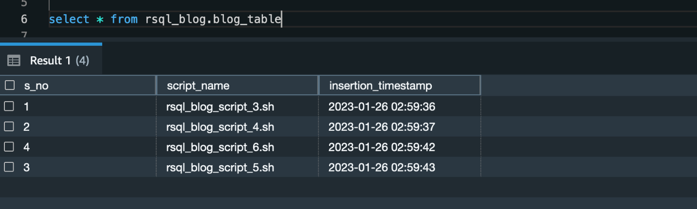
You can check the logs of the RSQL job in the CloudWatch log group (/ops/rsql-logs/) and also the run status of the workflow in the workflow audit DynamoDB table (rsql-blog-rsql-workflow-audit-table).
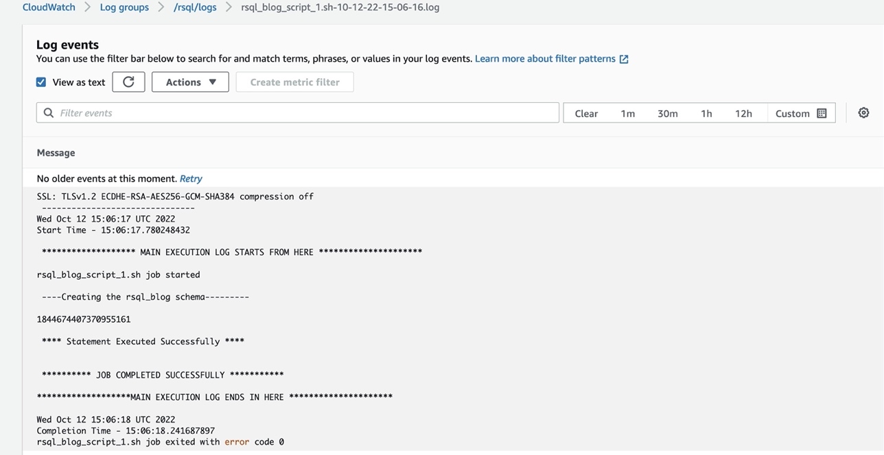

Clean up
To avoid ongoing charges for the resources that you created, delete them. AWS CDK deletes all resources except data resources such as DynamoDB tables.
- First, delete all AWS CDK stacks
- On the DynamoDB console, select the following tables and delete them:
rsql-blog-rsql-config-tablersql-blog-rsql-job-audit-tablersql-blog-rsql-workflow-audit-table
Conclusion
You can use Amazon Redshift RSQL, Systems Manager, EC2 instances, and Step Functions to create a modern and cost-effective orchestration framework for ETL workflows. There is no overhead to create and manage different state machines for each of your ETL workflow. In this post, we demonstrated how to use this configuration-based generic orchestration framework to trigger complex RSQL-based ETL workflows.
You can also trigger an email notification through Amazon Simple Notification Service (Amazon SNS) within the state machine to the notify the operations team of the completion status of the ETL process. Further, you can achieve a event-driven ETL orchestration framework by using EventBridge to start the workflow trigger lambda function.
About the Authors
 Akhil is a Data Analytics Consultant at AWS Professional Services. He helps customers design & build scalable data analytics solutions and migrate data pipelines and data warehouses to AWS. In his spare time, he loves travelling, playing games and watching movies.

Ramesh Raghupathy is a Senior Data Architect with WWCO ProServe at AWS. He works with AWS customers to architect, deploy, and migrate to data warehouses and data lakes on the AWS Cloud. While not at work, Ramesh enjoys traveling, spending time with family, and yoga.
 Raza Hafeez is a Senior Data Architect within the Shared Delivery Practice of AWS Professional Services. He has over 12 years of professional experience building and optimizing enterprise data warehouses and is passionate about enabling customers to realize the power of their data. He specializes in migrating enterprise data warehouses to AWS Modern Data Architecture.
 Dipal Mahajan is a Lead Consultant with Amazon Web Services based out of India, where he guides global customers to build highly secure, scalable, reliable, and cost-efficient applications on the cloud. He brings extensive experience on Software Development, Architecture and Analytics from industries like finance, telecom, retail and healthcare.
We often need our text search to be agnostic of accent marks. Accent-insensitive search, also called diacritics-agnostic search, is where search results are the same for queries that may or may not contain Latin characters such as à, è, Ê, ñ, and ç. Diacritics are English letters with an accent to mark a difference in pronunciation. In recent years, words with diacritics have trickled into the mainstream English language, such as café or protégé. Well, touché! OpenSearch has the answer!
OpenSearch is a scalable, flexible, and extensible open-source software suite for your search workload. OpenSearch can be deployed in three different modes: the self-managed open-source OpenSearch, the managed Amazon OpenSearch Service, and Amazon OpenSearch Serverless. All three deployment modes are powered by Apache Lucene, and offer text analytics using the Lucene analyzers.
In this post, we demonstrate how to perform accent-insensitive search using OpenSearch to handle diacritics.
Solution overview
Lucene Analyzers are Java libraries that are used to analyze text while indexing and searching documents. These analyzers consist of tokenizers and filters. The tokenizers split the incoming text into one or more tokens, and the filters are used to transform the tokens by modifying or removing the unnecessary characters.
OpenSearch supports custom analyzers, which enable you to configure different combinations of tokenizers and filters. It can consist of character filters, tokenizers, and token filters. In order to enable our diacritic-insensitive search, we configure custom analyzers that use the ASCII folding token filter.
ASCIIFolding is a method used to covert alphabetic, numeric, and symbolic Unicode characters that aren’t in the first 127 ASCII characters (the Basic Latin Unicode block) into their ASCII equivalents, if one exists. For example, the filter changes “à” to “a”. This allows search engines to return results agnostic of the accent.
In this post, we configure accent-insensitive search using the ASCIIFolding filter supported in OpenSearch Service. We ingest a set of European movie names with diacritics and verify search results with and without the diacritics.
Create an index with a custom analyzer
We first create the index asciifold\_movies with custom analyzer custom\_asciifolding:
Ingest sample data
Next, we ingest sample data with Latin characters into the index asciifold\_movies:
Query the index
Now we query the asciifold\_movies index for words with and without Latin characters.
Our first query uses an accented character:
Our second query uses a spelling of the same word without the accent mark:
In the preceding queries, the search terms “fête” and “fete” return the same results:
Similarly, try comparing results for “señora” and “senora” or “sorcière” and “sorciere.” The accent-insensitive results are due to the ASCIIFolding filter used with the custom analyzers.
Enable aggregations for fields with accents
Now that we have enabled accent-insensitive search, let’s look at how we can make aggregations work with accents.
Try the following query on the index:
We get the following response:
Create accent-insensitive aggregations using a normalizer
In the previous example, the aggregation returns two different buckets, one for “Jour de fête” and one for “Jour de fete.” We can enable aggregations to create one bucket for the field, regardless of the diacritics. This is achieved using the normalizer filter.
The normalizer supports a subset of character and token filters. Using just the defaults, the normalizer filter is a simple way to standardize Unicode text in a language-independent way for search, thereby standardizing different forms of the same character in Unicode and allowing diacritic-agnostic aggregations.
Let’s modify the index mapping to include the normalizer. Delete the previous index, then create a new index with the following mapping and ingest the same dataset:
After you ingest the same dataset, try the following query:
We get the following results:
Now we compare the results, and we can see the aggregations with term “Jour de fête” and “Jour de fete” are rolled up into one bucket with doc\_count=2.
Summary
In this post, we showed how to enable accent-insensitive search and aggregations by designing the index mapping to do ASCII folding for search tokens and normalize the keyword field for aggregations. You can use the OpenSearch query DSL to implement a range of search features, providing a flexible foundation for structured and unstructured search applications. The Open Source OpenSearch community has also extended the product to enable support for natural language processing, machine learning algorithms, custom dictionaries, and a wide variety of other plugins.
If you have feedback about this post, submit it in the comments section. If you have questions about this post, start a new thread on the Amazon OpenSearch Service forum or contact AWS Support.
About the Author
 Aruna Govindaraju is an Amazon OpenSearch Specialist Solutions Architect and has worked with many commercial and open-source search engines. She is passionate about search, relevancy, and user experience. Her expertise with correlating end-user signals with search engine behavior has helped many customers improve their search experience. Her favorite pastime is hiking the New England trails and mountains.
An event-driven architecture is a software design pattern in which decoupled applications can asynchronously publish and subscribe to events via an event broker. By promoting loose coupling between components of a system, an event-driven architecture leads to greater agility and can enable components in the system to scale independently and fail without impacting other services. AWS has many services to build solutions with an event-driven architecture, such as Amazon EventBridge, Amazon Simple Notification Service (Amazon SNS), Amazon Simple Queue Service (Amazon SQS), and AWS Lambda.
Amazon Elastic Kubernetes Service (Amazon EKS) is becoming a popular choice among AWS customers to host long-running analytics and AI or machine learning (ML) workloads. By containerizing your data processing tasks, you can simply deploy them into Amazon EKS as Kubernetes jobs and use Kubernetes to manage underlying computing compute resources. For big data processing, which requires distributed computing, you can use Spark on Amazon EKS. Amazon EMR on EKS, a managed Spark framework on Amazon EKS, enables you to run Spark jobs with benefits of scalability, portability, extensibility, and speed. With EMR on EKS, the Spark jobs run using the Amazon EMR runtime for Apache Spark, which increases the performance of your Spark jobs so that they run faster and cost less than open-source Apache Spark.
Data processes require a workflow management to schedule jobs and manage dependencies between jobs, and require monitoring to ensure that the transformed data is always accurate and up to date. One popular orchestration tool for managing workflows is Apache Airflow, which can be installed in Amazon EKS. Alternatively, you can use the AWS-managed version, Amazon Managed Workflows for Apache Airflow (Amazon MWAA). Another option is to use AWS Step Functions, which is a serverless workflow service that integrates with EMR on EKS and EventBridge to build event-driven workflows.
In this post, we demonstrate how to build an event-driven data pipeline using AWS Controllers for Kubernetes (ACK) and EMR on EKS. We use ACK to provision and configure serverless AWS resources, such as EventBridge and Step Functions. Triggered by an EventBridge rule, Step Functions orchestrates jobs running in EMR on EKS. With ACK, you can use the Kubernetes API and configuration language to create and configure AWS resources the same way you create and configure a Kubernetes data processing job. Because most of the managed services are serverless, you can build and manage your entire data pipeline using the Kubernetes API with tools such as kubectl.
Solution overview
ACK lets you define and use AWS service resources directly from Kubernetes, using the Kubernetes Resource Model (KRM). The ACK project contains a series of service controllers, one for each AWS service API. With ACK, developers can stay in their familiar Kubernetes environment and take advantage of AWS services for their application-supporting infrastructure. In the post Microservices development using AWS controllers for Kubernetes (ACK) and Amazon EKS blueprints, we show how to use ACK for microservices development.
In this post, we show how to build an event-driven data pipeline using ACK controllers for EMR on EKS, Step Functions, EventBridge, and Amazon Simple Storage Service (Amazon S3). We provision an EKS cluster with ACK controllers using Terraform modules. We create the data pipeline with the following steps:
- Create the emr-data-team-a namespace and bind it with the virtual cluster my-ack-vc in Amazon EMR by using the ACK controller.
- Use the ACK controller for Amazon S3 to create an S3 bucket. Upload the sample Spark scripts and sample data to the S3 bucket.
- Use the ACK controller for Step Functions to create a Step Functions state machine as an EventBridge rule target based on Kubernetes resources defined in YAML manifests.
- Use the ACK controller for EventBridge to create an EventBridge rule for pattern matching and target routing.
The pipeline is triggered when a new script is uploaded. An S3 upload notification is sent to EventBridge and, if it matches the specified rule pattern, triggers the Step Functions state machine. Step Functions calls the EMR virtual cluster to run the Spark job, and all the Spark executors and driver are provisioned inside the emr-data-team-a namespace. The output is saved back to the S3 bucket, and the developer can check the result on the Amazon EMR console.
The following diagram illustrates this architecture.

Prerequisites
Ensure that you have the following tools installed locally:
Deploy the solution infrastructure
Because each ACK service controller requires different AWS Identity and Access Management (IAM) roles for managing AWS resources, it’s better to use an automation tool to install the required service controllers. For this post, we use Amazon EKS Blueprints for Terraform and the AWS EKS ACK Addons Terraform module to provision the following components:
- A new VPC with three private subnets and three public subnets
- An internet gateway for the public subnets and a NAT Gateway for the private subnets
- An EKS cluster control plane with one managed node group
- Amazon EKS-managed add-ons:
VPC\_CNI,CoreDNS, andKube\_Proxy - ACK controllers for EMR on EKS, Step Functions, EventBridge, and Amazon S3
- IAM execution roles for EMR on EKS, Step Functions, and EventBridge
Let’s start by cloning the GitHub repo to your local desktop. The module eks\_ack\_addons in addon.tf is for installing ACK controllers. ACK controllers are installed by using helm charts in the Amazon ECR public galley. See the following code:
The following screenshot shows an example of our output. emr\_on\_eks\_role\_arn is the ARN of the IAM role created for Amazon EMR running Spark jobs in the emr-data-team-a namespace in Amazon EKS. stepfunction\_role\_arn is the ARN of the IAM execution role for the Step Functions state machine. eventbridge\_role\_arn is the ARN of the IAM execution role for the EventBridge rule.

The following command updates kubeconfig on your local machine and allows you to interact with your EKS cluster using kubectl to validate the deployment:
Test your access to the EKS cluster by listing the nodes:
Now we’re ready to set up the event-driven pipeline.
Create an EMR virtual cluster
Let’s start by creating a virtual cluster in Amazon EMR and link it with a Kubernetes namespace in EKS. By doing that, the virtual cluster will use the linked namespace in Amazon EKS for running Spark workloads. We use the file emr-virtualcluster.yaml. See the following code:
Let’s apply the manifest by using the following kubectl command:
You can navigate to the Virtual clusters page on the Amazon EMR console to see the cluster record.
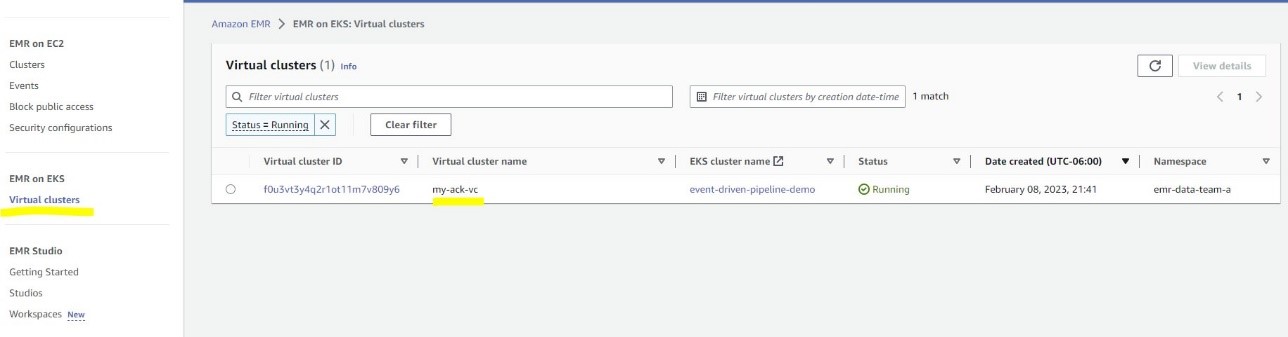
Create an S3 bucket and upload data
Next, let’s create a S3 bucket for storing Spark pod templates and sample data. We use the s3.yaml file. See the following code:
If you don’t see the bucket, you can check the log from the ACK S3 controller pod for details. The error is mostly caused if a bucket with the same name already exists. You need to change the bucket name in s3.yaml as well as in eventbridge.yaml and sfn.yaml. You also need to update upload-inputdata.sh and upload-spark-scripts.sh with the new bucket name.
Run the following command to upload the input data and pod templates:
The sparkjob-demo-bucket S3 bucket is created with two folders: input and scripts.
Create a Step Functions state machine
The next step is to create a Step Functions state machine that calls the EMR virtual cluster to run a Spark job, which is a sample Python script to process the New York City Taxi Records dataset. You need to define the Spark script location and pod templates for the Spark driver and executor in the StateMachine object .yaml file. Let’s make the following changes (highlighted) in sfn.yaml first:
- Replace the value for
roleARNwithstepfunctions\_role\_arn - Replace the value for
ExecutionRoleArnwithemr\_on\_eks\_role\_arn - Replace the value for
VirtualClusterIdwith your virtual cluster ID - Optionally, replace
sparkjob-demo-bucketwith your bucket name
See the following code:
You can get your virtual cluster ID from the Amazon EMR console or with the following command:
Then apply the manifest to create the Step Functions state machine:
Create an EventBridge rule
The last step is to create an EventBridge rule, which is used as an event broker to receive event notifications from Amazon S3. Whenever a new file, such as a new Spark script, is created in the S3 bucket, the EventBridge rule will evaluate (filter) the event and invoke the Step Functions state machine if it matches the specified rule pattern, triggering the configured Spark job.
Let’s use the following command to get the ARN of the Step Functions state machine we created earlier:
Then, update eventbridge.yaml with the following values:
- Under targets, replace the value for roleARN with
eventbridge\_role\_arn
Under targets, replace arn with your sfn\_arn
- Optionally, in eventPattern, replace
sparkjob-demo-bucketwith your bucket name
See the following code:
By applying the EventBridge configuration file, an EventBridge rule is created to monitor the folder scripts in the S3 bucket sparkjob-demo-bucket:
For simplicity, the dead-letter queue is not set and maximum retry attempts is set to 0. For production usage, set them based on your requirements. For more information, refer to Event retry policy and using dead-letter queues.
Test the data pipeline
To test the data pipeline, we trigger it by uploading a Spark script to the S3 bucket scripts folder using the following command:
The upload event triggers the EventBridge rule and then calls the Step Functions state machine. You can go to the State machines page on the Step Functions console and choose the job run-spark-job-ack to monitor its status.

For the Spark job details, on the Amazon EMR console, choose Virtual clusters in the navigation pane, and then choose my-ack-vc. You can review all the job run history for this virtual cluster. If you choose Spark UI in any row, you’re redirected the Spark history server for more Spark driver and executor logs.
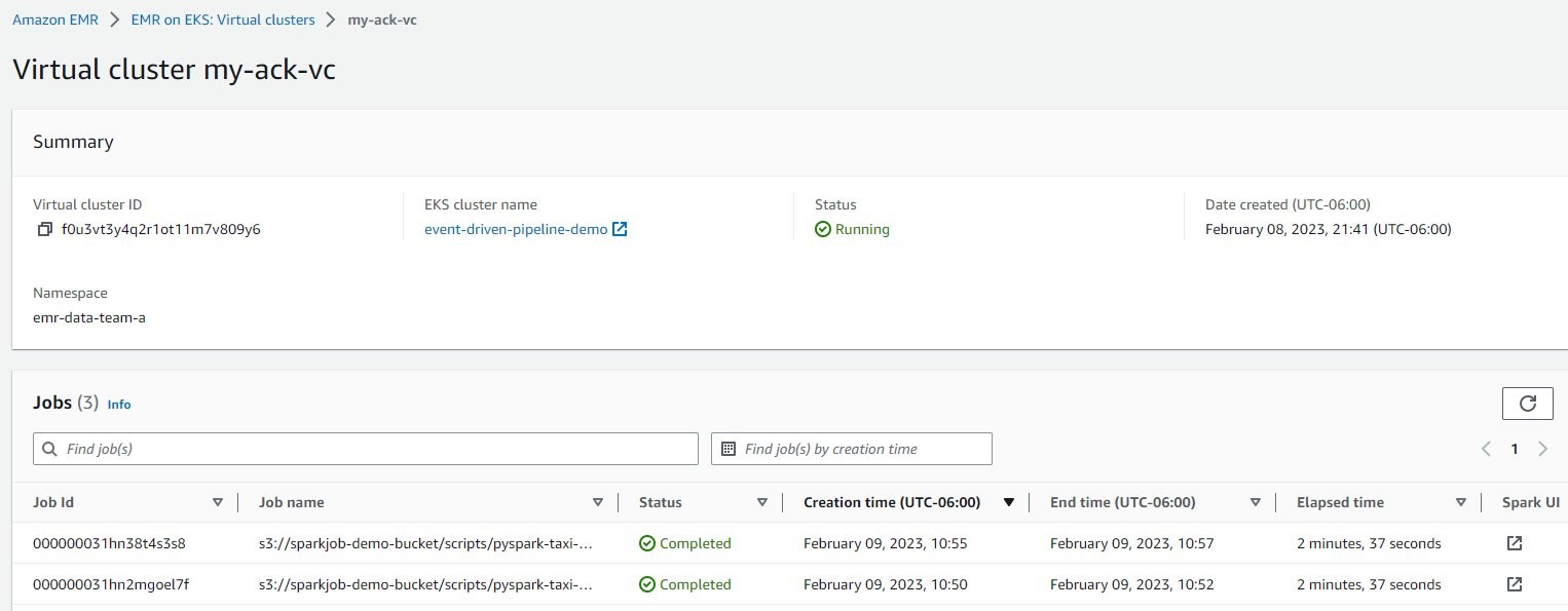
Clean up
To clean up the resources created in the post, use the following code:
Conclusion
This post showed how to build an event-driven data pipeline purely with native Kubernetes API and tooling. The pipeline uses EMR on EKS as compute and uses serverless AWS resources Amazon S3, EventBridge, and Step Functions as storage and orchestration in an event-driven architecture. With EventBridge, AWS and custom events can be ingested, filtered, transformed, and reliably delivered (routed) to more than 20 AWS services and public APIs (webhooks), using human-readable configuration instead of writing undifferentiated code. EventBridge helps you decouple applications and achieve more efficient organizations using event-driven architectures, and has quickly become the event bus of choice for AWS customers for many use cases, such as auditing and monitoring, application integration, and IT automation.
By using ACK controllers to create and configure different AWS services, developers can perform all data plane operations without leaving the Kubernetes platform. Also, developers only need to maintain the EKS cluster because all the other components are serverless.
As a next step, clone the GitHub repository to your local machine and test the data pipeline in your own AWS account. You can modify the code in this post and customize it for your own needs by using different EventBridge rules or adding more steps in Step Functions.
About the authors
 Victor Gu is a Containers and Serverless Architect at AWS. He works with AWS customers to design microservices and cloud native solutions using Amazon EKS/ECS and AWS serverless services. His specialties are Kubernetes, Spark on Kubernetes, MLOps and DevOps.
 Michael Gasch is a Senior Product Manager for AWS EventBridge, driving innovations in event-driven architectures. Prior to AWS, Michael was a Staff Engineer at the VMware Office of the CTO, working on open-source projects, such as Kubernetes and Knative, and related distributed systems research.
 Peter Dalbhanjan is a Solutions Architect for AWS based in Herndon, VA. Peter has a keen interest in evangelizing AWS solutions and has written multiple blog posts that focus on simplifying complex use cases. At AWS, Peter helps with designing and architecting variety of customer workloads.
In a data warehouse, a dimension is a structure that categorizes facts and measures in order to enable users to answer business questions. To illustrate an example, in a typical sales domain, customer, time or product are dimensions and sales transactions is a fact. Attributes within the dimension can change over time—a customer can change their address, an employee can move from a contractor position to a full-time position, or a product can have multiple revisions to it. A slowly changing dimension (SCD) is a data warehousing concept that contains relatively static data that can change slowly over a period of time. There are three major types of SCDs maintained in data warehousing: Type 1 (no history), Type 2 (full history), and Type 3 (limited history). Change data capture (CDC) is a characteristic of a database that provides an ability to identify the data that changed between two database loads, so that an action can be performed on the changed data.
As organizations across the globe are modernizing their data platforms with data lakes on Amazon Simple Storage Service (Amazon S3), handling SCDs in data lakes can be challenging. It becomes even more challenging when source systems don’t provide a mechanism to identify the changed data for processing within the data lake and makes the data processing highly complex if the data source happens to be semi-structured instead of a database. The key objective while handling Type 2 SCDs is to define the start and end dates to the dataset accurately to track the changes within the data lake, because this provides the point-in-time reporting capability for the consuming applications.
In this post, we focus on demonstrating how to identify the changed data for a semi-structured source (JSON) and capture the full historical data changes (SCD Type 2) and store them in an S3 data lake, using AWS Glue and open data lake format Delta.io. This implementation supports the following use cases:
- Track Type 2 SCDs with start and end dates to identify the current and full historical records and a flag to identify the deleted records in the data lake (logical deletes)
- Use consumption tools such as Amazon Athena to query historical records seamlessly
Solution overview
This post demonstrates the solution with an end-to-end use case using a sample employee dataset. The dataset represents employee details such as ID, name, address, phone number, contractor or not, and more. To demonstrate the SCD implementation, consider the following assumptions:
- The data engineering team receives daily files that are full snapshots of records and don’t contain any mechanism to identify source record changes
- The team is tasked with implementing SCD Type 2 functionality for identifying new, updated, and deleted records from the source, and to preserve the historical changes in the data lake
- Because the source systems don’t provide the CDC capability, a mechanism needs to be developed to identify the new, updated, and deleted records and persist them in the data lake layer
The architecture is implemented as follows:
- Source systems ingest files in the S3 landing bucket (this step is mimicked by generating the sample records using the provided AWS Lambda function into the landing bucket)
- An AWS Glue job (Delta job) picks the source data file and processes the changed data from the previous file load (new inserts, updates to the existing records, and deleted records from the source) into the S3 data lake (processed layer bucket)
- The architecture uses the open data lake format (Delta), and builds the S3 data lake as a Delta Lake, which is mutable, because the new changes can be updated, new inserts can be appended, and source deletions can be identified accurately and marked with a
delete\_flagvalue - An AWS Glue crawler catalogs the data, which can be queried by Athena
The following diagram illustrates our architecture.

Prerequisites
Before you get started, make sure you have the following prerequisites:
- An AWS account
- Appropriate AWS Identity and Access Management (IAM) permissions to deploy AWS CloudFormation stack resources
Deploy the solution
For this solution, we provide a CloudFormation template that sets up the services included in the architecture, to enable repeatable deployments. This template creates the following resources:
- Two S3 buckets: a landing bucket for storing sample employee data and a processed layer bucket for the mutable data lake (Delta Lake)
- A Lambda function to generate sample records
- An AWS Glue extract, transform, and load (ETL) job to process the source data from the landing bucket to the processed bucket
To deploy the solution, complete the following steps:
- Choose Launch Stack to launch the CloudFormation stack:

- Enter a stack name.
- Select I acknowledge that AWS CloudFormation might create IAM resources with custom names.
- Choose Create stack.
After the CloudFormation stack deployment is complete, navigate to AWS CloudFormation console to note the following resources on the Outputs tab:
- Data lake resources – The S3 buckets
scd-blog-landing-xxxxandscd-blog-processed-xxxx(referred to asscd-blog-landingandscd-blog-processedin the subsequent sections in this post) - Sample records generator Lambda function –
SampleDataGenaratorLambda-<CloudFormation Stack Name>(referred to asSampleDataGeneratorLambda) - AWS Glue Data Catalog database –
deltalake\_xxxxxx(referred to asdeltalake) - AWS Glue Delta job –
<CloudFormation-Stack-Name>-src-to-processed(referred to assrc-to-processed)
Note that deploying the CloudFormation stack in your account incurs AWS usage charges.
Test SCD Type 2 implementation
With the infrastructure in place, you’re ready to test out the overall solution design and query historical records from the employee dataset. This post is designed to be implemented for a real customer use case, where you get full snapshot data on a daily basis. We test the following aspects of SCD implementation:
- Run an AWS Glue job for the initial load
- Simulate a scenario where there are no changes to the source
- Simulate insert, update, and delete scenarios by adding new records, and modifying and deleting existing records
- Simulate a scenario where the deleted record comes back as a new insert
Generate a sample employee dataset
To test the solution, and before you can start your initial data ingestion, the data source needs to be identified. To simplify that step, a Lambda function has been deployed in the CloudFormation stack you just deployed.

Open the function and configure a test event, with the default hello-world template event JSON as seen in the following screenshot. Provide an event name without any changes to the template and save the test event.

Choose Test to invoke a test event, which invokes the Lambda function to generate the sample records.

When the Lambda function completes its invocation, you will be able to see the following sample employee dataset in the landing bucket.

Run the AWS Glue job
Confirm if you see the employee dataset in the path s3://scd-blog-landing/dataset/employee/. You can download the dataset and open it in a code editor such as VS Code. The following is an example of the dataset:
Download the dataset and keep it ready, because you will modify the dataset for future use cases to simulate the inserts, updates, and deletes. The sample dataset generated for you will be entirely different than what you see in the preceding example.
To run the job, complete the following steps:
- On the AWS Glue console, choose Jobs in the navigation pane.
- Choose the job
src-to-processed. - On the Runs tab, choose Run.
When the AWS Glue job is run for the first time, the job reads the employee dataset from the landing bucket path and ingests the data to the processed bucket as a Delta table.

When the job is complete, you can create a crawler to see the initial data load. The following screenshot shows the database available on the Databases page.

- Choose Crawlers in the navigation pane.
- Choose Create crawler.

- Name your crawler
delta-lake-crawler, then choose Next.

- Select Not yet for data already mapped to AWS Glue tables.
- Choose Add a data source.

- On the Data source drop-down menu, choose Delta Lake.
- Enter the path to the Delta table.
- Select Create Native tables.
- Choose Add a Delta Lake data source.

- Choose Next.

- Choose the role that was created by the CloudFormation template, then choose Next.

- Choose the database that was created by the CloudFormation template, then choose Next.

- Choose Create crawler.

- Select your crawler and choose Run.

Query the data
After the crawler is complete, you can see the table it created.

To query the data, complete the following steps:
- Choose the employee table and on the Actions menu, choose View data.

You’re redirected to the Athena console. If you don’t have the latest Athena engine, create a new Athena workgroup with the latest Athena engine.
- Under Administration in the navigation pane, choose Workgroups.

- Choose Create workgroup.

- Provide a name for the workgroup, such as
DeltaWorkgroup. - Select Athena SQL as the engine, and choose Athena engine version 3 for Query engine version.

- Choose Create workgroup.

- After you create the workgroup, select the workgroup (
DeltaWorkgroup) on the drop-down menu in the Athena query editor.

- Run the following query on the
employeetable:
Note: Update the correct database name from the CloudFormation outputs before running the above query.
You can observe that the employee table has 25 records. The following screenshot shows the total employee records with some sample records.

The Delta table is stored with an emp\_key, which is unique to each and every change and is used to track the changes. The emp\_key is created for every insert, update, and delete, and can be used to find all the changes pertaining to a single emp\_id.
The emp\_key is created using the SHA256 hashing algorithm, as shown in the following code:
Perform inserts, updates, and deletes
Before making changes to the dataset, let’s run the same job one more time. Assuming that the current load from the source is the same as the initial load with no changes, the AWS Glue job shouldn’t make any changes to the dataset. After the job is complete, run the previous Select query in the Athena query editor and confirm that there are still 25 active records with the following values:
- All 25 records with the column
isCurrent=true - All 25 records with the column
end\_date=Null - All 25 records with the column
delete\_flag=false
After you confirm the previous job run with these values, let’s modify our initial dataset with the following changes:
- Change the
isContractorflag tofalse(change it totrueif your dataset already showsfalse) foremp\_id=12. - Delete the entire row where
emp\_id=8(make sure to save the record in a text editor, because we use this record in another use case). - Copy the row for
emp\_id=25and insert a new row. Change theemp\_idto be26, and make sure to change the values for other columns as well.
After we make these changes, the employee source dataset looks like the following code (for readability, we have only included the changed records as described in the preceding three steps):
- Now, upload the changed
fake\_emp\_data.jsonfile to the same source prefix.

- After you upload the changed employee dataset to Amazon S3, navigate to the AWS Glue console and run the job.
- When the job is complete, run the following query in the Athena query editor and confirm that there are 27 records in total with the following values:
Note: Update the correct database name from the CloudFormation output before running the above query.

- Run another query in the Athena query editor and confirm that there are 4 records returned with the following values:
Note: Update the correct database name from the CloudFormation output before running the above query.

You will see two records for emp\_id=12:
- One
emp\_id=12record with the following values (for the record that was ingested as part of the initial load):emp\_key=44cebb094ef289670e2c9325d5f3e4ca18fdd53850b7ccd98d18c7a57cb6d4b4isCurrent=falsedelete\_flag=falseend\_date=’2023-03-02’
- A second
emp\_id=12record with the following values (for the record that was ingested as part of the change to the source):emp\_key=b60547d769e8757c3ebf9f5a1002d472dbebebc366bfbc119227220fb3a3b108isCurrent=truedelete\_flag=falseend\_date=Null(or empty string)
The record for emp\_id=8 that was deleted in the source as part of this run will still exist but with the following changes to the values:
isCurrent=falseend\_date=’2023-03-02’delete\_flag=true
The new employee record will be inserted with the following values:
emp\_id=26isCurrent=trueend\_date=NULL(or empty string)delete\_flag=false
Note that the emp\_key values in your actual table may be different than what is provided here as an example.
- For the deletes, we check for the emp\_id from the base table along with the new source file and inner join the emp\_key.
- If the condition evaluates to true, we then check if the employee base table emp\_key equals the new updates emp\_key, and get the current, undeleted record (isCurrent=true and delete\_flag=false).
- We merge the delete changes from the new file with the base table for all the matching delete condition rows and update the following:
isCurrent=falsedelete\_flag=trueend\_date=current\_date
See the following code:
- For both the updates and the inserts, we check for the condition if the base table
employee.emp\_idis equal to thenew changes.emp\_idand theemployee.emp\_keyis equal tonew changes.emp\_key, while only retrieving the current records. - If this condition evaluates to
true, we then get the current record (isCurrent=trueanddelete\_flag=false). - We merge the changes by updating the following:
- If the second condition evaluates to
true:isCurrent=falseend\_date=current\_date
- Or we insert the entire row as follows if the second condition evaluates to
false:emp\_id=new record’s emp\_keyemp\_key=new record’s emp\_keyfirst\_name=new record’s first\_namelast\_name=new record’s last\_nameaddress=new record’s addressphone\_number=new record’s phone\_numberisContractor=new record’s isContractorstart\_date=current\_dateend\_date=NULL(or empty string)isCurrent=truedelete\_flag=false
- If the second condition evaluates to
See the following code:
As a last step, let’s bring back the deleted record from the previous change to the source dataset and see how it is reinserted into the employee table in the data lake and observe how the complete history is maintained.
Let’s modify our changed dataset from the previous step and make the following changes.
- Add the deleted
emp\_id=8back to the dataset.
After making these changes, my employee source dataset looks like the following code (for readability, we have only included the added record as described in the preceding step):
{"emp\_id":8,"first\_name":"Teresa","last\_name":"Estrada","Address":"339 Scott Valley\nGonzalesfort, PA 18212","phone\_number":"435-600-3162","isContractor":false}
- Upload the changed employee dataset file to the same source prefix.

- After you upload the changed
fake\_emp\_data.jsondataset to Amazon S3, navigate to the AWS Glue console and run the job again. - When the job is complete, run the following query in the Athena query editor and confirm that there are 28 records in total with the following values:
Note: Update the correct database name from the CloudFormation output before running the above query.

- Run the following query and confirm there are 5 records:

You will see two records for emp\_id=8:
- One
emp\_id=8record with the following values (the old record that was deleted):emp\_key=536ba1ba5961da07863c6d19b7481310e64b58b4c02a89c30c0137a535dbf94disCurrent=falsedeleted\_flag=trueend\_date=’2023-03-02’
- Another
emp\_id=8record with the following values (the new record that was inserted in the last run):emp\_key=536ba1ba5961da07863c6d19b7481310e64b58b4c02a89c30c0137a535dbf94disCurrent=truedeleted\_flag=falseend\_date=NULL(or empty string)
The emp\_key values in your actual table may be different than what is provided here as an example. Also note that because this is a same deleted record that was reinserted in the subsequent load without any changes, there will be no change to the emp\_key.
End-user sample queries
The following are some sample end-user queries to demonstrate how the employee change data history can be traversed for reporting:
- Query 1 – Retrieve a list of all the employees who left the organization in the current month (for example, March 2023).

The preceding query would return two employee records who left the organization.
- Query 2 – Retrieve a list of new employees who joined the organization in the current month (for example, March 2023).
Note: Update the correct database name from the CloudFormation output before running the above query.

The preceding query would return 23 active employee records who joined the organization.
- Query 3 – Find the history of any given employee in the organization (in this case employee 18).
Note: Update the correct database name from the CloudFormation output before running the above query.

In the preceding query, we can observe that employee 18 had two changes to their employee records before they left the organization.
Note that the data results provided in this example are different than what you will see in your specific records based on the sample data generated by the Lambda function.
Clean up
When you have finished experimenting with this solution, clean up your resources, to prevent AWS charges from being incurred:
- Empty the S3 buckets.
- Delete the stack from the AWS CloudFormation console.
Conclusion
In this post, we demonstrated how to identify the changed data for a semi-structured data source and preserve the historical changes (SCD Type 2) on an S3 Delta Lake, when source systems are unable to provide the change data capture capability, with AWS Glue. You can further extend this solution to enable downstream applications to build additional customizations from CDC data captured in the data lake.
Additionally, you can extend this solution as part of an orchestration using AWS Step Functions or other commonly used orchestrators your organization is familiar with. You can also extend this solution by adding partitions where appropriate. You can also maintain the delta table by compacting the small files.
About the authors
 Nith Govindasivan, is a Data Lake Architect with AWS Professional Services, where he helps onboarding customers on their modern data architecture journey through implementing Big Data & Analytics solutions. Outside of work, Nith is an avid Cricket fan, watching almost any cricket during his spare time and enjoys long drives, and traveling internationally.
 Vijay Velpula is a Data Architect with AWS Professional Services. He helps customers implement Big Data and Analytics Solutions. Outside of work, he enjoys spending time with family, traveling, hiking and biking.
 Sriharsh Adari is a Senior Solutions Architect at Amazon Web Services (AWS), where he helps customers work backwards from business outcomes to develop innovative solutions on AWS. Over the years, he has helped multiple customers on data platform transformations across industry verticals. His core area of expertise include Technology Strategy, Data Analytics, and Data Science. In his spare time, he enjoys playing sports, binge-watching TV shows, and playing Tabla.
Data lakes have come a long way, and there’s been tremendous innovation in this space. Today’s modern data lakes are cloud native, work with multiple data types, and make this data easily available to diverse stakeholders across the business. As time has gone by, data lakes have grown significantly and have evolved to data meshes as a way to scale. Thoughtworks defines a data mesh as “a shift in a modern distributed architecture that applies platform thinking to create self-serve data infrastructure, treating data as the product.”
Data mesh advocates for decentralized ownership and delivery of enterprise data management systems that benefit several personas. Data producers can use the data mesh platform to create datasets and share them across business teams to ensure data availability, reliability, and interoperability across functions and data subject areas. Data consumers now have better data sharing with data mesh and federation across business units without compromising data security. The data governance team can support distributed data, where all data is accessible to those with the proper authority to access it. With data mesh, data doesn’t have to be consolidated into a single data lake or account and can remain within different databases and data lakes. An essential capability needed in such a data lake architecture is the ability to continuously understand changes in the data lakes in various other domains and make those available to data consumers. Without such a capability, manual work is needed to understand producers’ updates and make them available to consumers and governance.
AWS customers use a modern data architecture to facilitate governance and data sharing across logical or physical governance boundaries to create data domains aligned to lines of business. Each line of business creates and manages their dataset on Amazon Simple Storage Service (Amazon S3) and uses AWS Glue crawlers to discover new datasets and register them to the AWS Glue Data Catalog, add new tables and partitions, and detect schema changes. These datasets are shared with data consumers that access the data using services like Amazon Athena, Amazon Redshift, Amazon EMR, and more.
In the post Introducing AWS Glue crawlers using AWS Lake Formation permission management, we introduced a new set of capabilities in AWS Glue crawlers and AWS Lake Formation that simplifies crawler setup and supports centralized permissions for in-account and cross-account crawling of S3 data lakes. In this post, we demonstrate the same capability for a data mesh architecture in which we establish a central governance layer to catalog the data owned by the data producer and share it with the data consumer for ease of discovery. The AWS Glue crawler cross-account capability allows you to crawl data sources in different producer accounts while still having those changes cataloged in a centralized governance account. Customers prefer the central governance experience over writing bucket policies separately in each bucket owning the account of a data mesh producer. To build a data mesh architecture, now you can author permissions in a single Lake Formation governance to manage access to data locations and crawlers spanning multiple accounts in the data mesh.
According to the Allstate Corporation:
“By leveraging the power of AWS Lake Formation in our modern data architecture, we will be able to further unlock the potential of our data and empower our analytics community to drive innovation and build data-driven applications. The granular data access and collaboration provided by this architecture will enable us to build a truly unified data and analytics experience, bringing us one step closer to realizing our vision of becoming a fully data-driven enterprise.”
– Prashant Mehrotra, Director – Machine Learning and R&D, Allstate
In this post, we walk through the creation of a simplified data mesh architecture that shows how to use an AWS Glue crawler with Lake Formation to automate bringing changes from data producer domains to data consumers while maintaining centralized governance.
Solution overview
In a data mesh architecture, you have several producer accounts that own S3 buckets, several consumer accounts who wants to access shared datasets, and a central governance account to manage data shares between producers and consumers. This central governance account doesn’t own any S3 bucket or actual tables.
The following figure shows a simplified data mesh architecture with a single producer account, a centralized governance account, and a single consumer account. The data mesh producer account hosts the encrypted S3 bucket, which is shared with the central governance account. The central governance account registers the S3 bucket with Lake Formation using an AWS Identity and Access Management (IAM) role, which has permissions to the S3 bucket and AWS Key Management Service (AWS KMS). The central account creates the database for storing the dataset schema and shares it with the producer account. The producer account, as the S3 bucket owner, runs a crawler to crawl the buckets registered with the central account using Lake Formation permissions and populates the database. Now the shared database with new datasets are available to share with consumers in the data mesh. The central governance account can now share the database with a consumer admin, who can delegate access to other personas (such as data analysts) in the consumer account for data access.

In the following sections, we provide AWS CloudFormation templates to set up the resources in each account. Then we provide the steps to configure the crawler, manage permissions and sharing, and validate the solution by running queries with Athena.
Prerequisites
Complete the following steps in each account (producer, central governance, and consumer) to update the Data Catalog settings to use Lake Formation permissions to control catalog resources instead of IAM-based access control:
- Sign in to the Lake Formation console as admin.
- If this is the first time accessing the Lake Formation console, add yourself as the data lake administrator.

- In the navigation pane, under Data catalog, choose Settings.
- Uncheck Use only IAM access control for new databases.
- Uncheck Use only IAM access control for new tables in new databases.
- Keep Version 3 as the current cross-account version.
- Choose Save.
Set up resources in the central governance account
The CloudFormation template for the central account creates a CentralDataMeshOwner user assigned as Lake Formation admin. The CentralDataMeshOwner user in the central governance account performs the necessary steps to share the central catalogs with the producer and consumer accounts. The CentralDataMeshOwner user also sets up a custom Lake Formation service role to register the S3 data lake location. Complete the following steps:
- Log in to the central governance account console as IAM administrator.
- Choose Launch Stack to deploy the CloudFormation template:
- For DataMeshOwnerUserName, keep the default (
CentralDataMeshOwner). - For ProducerAWSAccount, enter the producer account ID.
- Create the stack.
- After the stack launches, on the AWS CloudFormation console, navigate to the Resources tab of the stack.
- Note down the value of
RegisterLocationServiceRole. - Choose the
LFUsersPasswordvalue to navigate to the AWS Secrets Manager console. - In the Secret value section, choose Retrieve secret value.
- Note down the secret value for the password for IAM user
CentralDataMeshOwner.
Set up resources in the producer account
The CloudFormation template for the producer account creates the following resources:
- IAM user
LOBProducerSteward - S3 bucket
retail-datalake-<producer account id >-<producer region> - KMS key used for bucket encryption
- Required S3 bucket policies to provide access to the central governance account
- AWS Glue crawler and crawler IAM role with necessary permissions
Complete the following steps:
- Log in to the producer account console as IAM administrator.
- Choose Launch Stack to deploy the CloudFormation template:
- For CentralAccountID, enter the central account ID.
- For CentralAccountLFServiceRole, enter the value of
RegisterLocationServiceRolefrom CloudFormation noted earlier. - Create the stack.
- When the stack is complete, on the AWS CloudFormation console, navigate to the Resources tab of the stack.
- Note down the
AWSGlueServiceRolevalue. - Choose the
ProducerStewardUserCredentialsvalue to navigate to the Secrets Manager console. - In the Secret value section, choose Retrieve secret value.
- Note down the secret value for the password for IAM user
LOBProducerSteward. - On the Amazon S3 console, check the bucket policies for
retail-datalake-<producer account id >-<producer region>and make sure it is shared with the central governance account IAM role.
This is required for registering the bucket with Lake Formation in the central account so that the account can manage the data sharing.
- On the AWS KMS console, check that the bucket is encrypted with the customer managed key and the key is shared with the central governance account.
Set up resources in the consumer account
The CloudFormation template for the consumer account creates the following resources:
- IAM user
ConsumerAdminUserassigned to the data lake admin - IAM user
LFBusinessAnalyst1 - S3 bucket for Athena output
- Athena workgroup
Complete the following steps:
- Log in to the consumer account console as IAM administrator.
- Choose Launch Stack to deploy the CloudFormation template:
- Create the stack.
- When the stack is complete, on the AWS CloudFormation console, navigate to the Resources tab of the stack.
- Choose the
AllConsumerUsersCredentialsvalue to navigate to the Secrets Manager console. - In the Secret value section, choose Retrieve secret value.
- Note down the secret value for the password for the IAM user
ConsumerAdminUser.
Now that all the accounts have been set up, we set up cross-account sharing on AWS with a central governance account to manage sharing of permissions across producers and consumers.
Configure the central governance account to manage sharing with the producer account
Sign in to the central governance account as CentralDataMeshOwner using the password noted earlier through the central governance account CloudFormation stack. Then complete the following steps:
- On Lake Formation console, choose Data lake locations under Register and ingest in the navigation pane.
- For Amazon S3 path, provide the path
retail-datalake-<producer account id >-<region>. - For IAM role, choose the IAM role created using the CloudFormation stack.
This role has permissions for the accessing the encrypted S3 bucket and its key. Do not choose the role AWSServiceRoleForLakeFormationDataAccess.
- Choose Register location.

- In the navigation pane, choose Databases.
- Choose Create database.
- For Database name¸ enter
datameshtestdatabase. - Choose Create database.
- In the navigation pane, choose Data locations and choose Grant.

- Select External account and provide the producer account for AWS account ID, AWS organization ID, or IAM principal ARN.
- For Storage location, provide the data lake bucket path.
- Select Grantable, then choose Grant.
- Choose Data lake permissions, then choose Grant.
- Select External accounts and provide the producer account number.
- For Databases, choose
datameshtestdatabase. - For Database permissions and Grantable permissions, select Create table, Alter, and Describe.
- Choose Grant.


Configure the crawler in the producer account to populate the schema
Sign in to producer account as LOBProducerSteward with the password noted earlier through the producer account CloudFormation stack, then complete the following steps:
- On the AWS RAM console, accept the pending resource share from the central account.
- On the Lake Formation console, choose Databases under Data catalog in the navigation pane.
- Choose
datameshtestdatabase, and on the Action menu, choose Create resource link. - For Resource link name, enter
datameshtestdatabaselink. - Choose Create.

- On the AWS Glue console, choose Crawlers in the navigation pane.
- Choose the crawler
CrossAccountCrawler-<accountid>. - Choose Edit, then choose Configure security settings.
- Select Use Lake Formation credentials for crawling S3 data source.
- Select In a different account and provide the account ID of the central governance account.
- Choose Next.

- Choose
datameshtestdatabaselinkas the database and choose Update.

- In the navigation pane, choose Data locations and choose Grant.
- Select My account, and choose the crawler IAM role for IAM users and roles.
- For Storage locations, choose the bucket
retail-datalake-<accountid>-<region>. - For Registered account location, enter the central account ID.
- Choose Grant.
 Alternatively, you can also use the AWS CLI to grant data location permission on bucket registered in central account to the crawler role using below command:
 For using CLI, refer to Installing or updating the latest version of the AWS CLI.
- In the navigation pane, choose Data lake permissions.
- Choose the crawler IAM role for the principal account.
- Choose
datameshtestdatabasefor the database. - For Database permissions, select Create, Describe, and Alter.
- Choose Grant.

- Choose the crawler IAM role for the principal account.
- Choose
datameshtestdatabaselinkfor the database. - For Resource link permissions, select Describe.
- Choose Grant.
- Run the crawler.
The following screenshot shows the details after a successful run.

When the crawler is complete, you can validate the table created under the database datameshtestdatabaselink.


This table is owned by the producer account and available in the central governance account under the shared database datameshtestdatabase. Now the data lake admin in the central governance account can share the database and populated table with the consumer account.
Configure the central governance account to manage sharing of read-only access with the consumer account
Sign in to the central governance account as CentralDataMeshOwner with the password noted earlier through the central governance account CloudFormation stack, then complete the following steps:
- Grant database permissions to the consumer account.
- For Principals, choose external account and provide <consumer accountID>
- For Databases, select
datameshtestdatabase. - For Database permissions, select Describe.
- For Grantable permissions¸ select Describe.
- Choose Grant.


- Grant table permissions to the consumer account.
- For Principals, choose external account and provide
<consumer accountID>. - For Databases, select
datameshtestdatabase. - For Tables, select
retail\_datalake\_<accountID>\_<region>. - For Table permissions, select Select and Describe.
- For Grantable permissions¸ select Select and Describe.
- Choose Grant.


Configure the consumer account as the consumer account data lake admin
Sign to the consumer account as ConsumerAdminUser with the password noted earlier through the consumer account CloudFormation stack. (Note that in the consumer account Lake Formation configuration, both ConsumerAdminUser and LFBusinessAnalyst1 have the same password.)
- On the AWS RAM console, accept the resource share from the central account.
- On the Lake Formation console, validate that the shared database datameshtestdatabase is available and create the resource link datameshtestdatabaselink using the shared database.
The following screenshot shows the details after the resource link is created.

- On the Lake Formation console, choose Grant.
- Choose LFBusinessAnalyst1 for IAM users and roles.
- Choose
datameshtestdatabasefor the database under Named data catalog resources. - Select Describe for Database permissions.
- On the Lake Formation console, choose Grant.
- Choose
LFBusinessAnalyst1for IAM users and roles. - Choose
datameshtestdatabaselinkfor the database under Named data catalog resources. - Select Describe for Resource link permissions.
- On the Lake Formation console, choose Grant.
- Choose
LFBusinessAnalyst1for IAM users and roles. - Choose
retail\_datalake\_<accountid>\_<region>for the table under Named data catalog resources. - Select Select and Describe for Table permissions.
Run queries in the consumer account
Sign to the consumer account console as LFBusinessAnalyst1 with the password noted earlier through the consumer account CloudFormation stack, then complete the following steps:
- On the Athena console, and choose
lfconsumer-workgroupas the Athena workgroup. - Run the following query to validate access:

We have successfully registered the dataset and created a Data Catalog in the central governance account. We crawled the data lake that was registered with the central governance account using Lake Formation permissions from the producer account and populated the schema. We granted Lake Formation permission on the database and table from the central account to the consumer user and validated consumer user access to the data using Athena.
Clean up
To avoid unwanted charges to your AWS account, delete the AWS resources:
- Sign in to the CloudFormation console as the IAM admin used for creating the CloudFormation stack in all three accounts.
- Delete the stacks you created.
Conclusion
In this post, we showed how to set up cross-account crawling using a central governance account with the new AWS Glue crawler capability of Lake Formation integration. This capability allows data producers to set up crawling capabilities in their own domain so that changes are seamlessly available to data governance and data consumers. Implementing a data mesh with AWS Glue crawlers, Lake Formation, Athena, and other analytical services provide a well-understood, performant, scalable, and cost-effective solution to integrate, prepare, and serve data.
If you have questions or suggestions, submit them in the comments section.
For more resources, refer to the following:
- Design a data mesh architecture using AWS Lake Formation and AWS Glue
- Introducing AWS Glue crawlers using AWS Lake Formation permission management
About the authors
 Sandeep Adwankar is a Senior Technical Product Manager at AWS. Based in the California Bay Area, he works with customers around the globe to translate business and technical requirements into products that enable customers to improve how they manage, secure, and access data.
 Srividya Parthasarathy is a Senior Big Data Architect on the AWS Lake Formation team. She enjoys building data mesh solutions and sharing them with the community.
 Piyali Kamra is a seasoned enterprise architect and a hands-on technologist who believes that building large scale enterprise systems is not an exact science but more like an art, in which tools and technologies must be carefully selected based on the team’s culture , strengths , weaknesses and risks , in tandem with having a futuristic vision as to how you want to shape your product a few years down the road.
Deep Pool Financial Solutions, an investor servicing and compliance solutions supplier, was looking to build key performance indicators to track its software tests, failures, and successful fixes to pinpoint the specific areas for improvement in its client software. Deep Pool was unable to access the large amounts of data that its project management software provided, so it used AWS to access, manage, and analyze that data more efficiently.
During a larger migration to the AWS Cloud, the company discovered Amazon QuickSight, a cloud-native, serverless business intelligence (BI) service that powers interactive dashboards that let companies make better data-driven decisions. With QuickSight, Deep Pool could democratize access to this unused data and pinpoint areas for improvement in its software development processes, thereby improving the overall quality of its software.
According to Brett Promisel, Chief Operating Officer for Deep Pool, the company wanted to manage the data that it was collecting from a BI point of view to help it make more informed decisions. Because word of mouth and high-quality software are critical in Deep Pool’s industry, the company wanted to add additional rigorous quality controls to its product development and testing so that it continues to provide top-notch, stable software that its clients can rely on.
In this post, we share how Deep Pool boosted its software quality control using QuickSight.
Enhancing software testing to with data-driven insights
Continuous improvement is a hallmark of leading organizations. Deep Pool wanted achieve greater software quality and decided to improve how it monitored and managed its software testing processes using data.
Typical development processes involve extensive testing. First, the original developer tests the code, and then the code is unit tested. Next, larger groups test the code. For all this testing to be successful and result in product improvement, it needs to be measured and tracked so that developers can learn from it and implement improvements during the development process.
Using QuickSight for data-driven insights, Deep Pool has implemented significant software testing and control. It can now count the number of bugs found or tests failed and time how long it took to create patches and repair issues. It can also better track its work backlog and the progress of functionality requests. Monitoring this information lets the company know that it has successfully implemented improvements, because a decreasing number of bugs over time is a strong indicator of quality control.
Monitoring development to increase efficiency
Better software test management benefits two groups: internal teams and external customers. Deep Pool can now log and communicate important information, such as when a request is made, how it’s being resolved or addressed, and how it’s being tested. In addition to helping internal teams streamline their processes, the company can also use this data to track communications with customers, which are also stored in its project management software. Such knowledge helps the company determine whether customer requests are being promptly addressed and identify common trends that require action on a larger scale.
Seven development teams at Deep Pool independently write the code for the components of the company’s software products, and they must integrate those components to create the final products. With the granularity of the data that is provided by QuickSight, Deep Pool can thoroughly analyze the development and testing of these products. The company now has the ability to trace software bugs down to their original coding, which makes it simple to quickly locate and address any issues that come up. Deep Pool can also measure the results of those mitigating actions and determine whether its repairs were successful.
Attention to detail helps Deep Pool improve software quality, leading to better products and customers who are more likely to give positive referrals.
“Amazon QuickSight is extremely valuable to us when performing quality control. We can now expose our whole development team to how we’re managing databases and servers and measuring performance in a more optimal way,” says Promisel.
Deep Pool has successfully proven that it can use QuickSight to measure its quality control to improve its software and, ultimately, better support its customers. Since the migration to AWS, the number of software issues discovered and logged has dropped by 57%.
The increased quality control that has come from the company’s focus on accessing all its data and optimizing its use has led to better efficiency, which results in the ability to expand its growth without increasing its costs.
“We should be able to increase our customer base without adding the equivalent costs. Making sure we are as efficient as possible lets me manage that way,” says Promisel.
Expanding into more data sources
Deep Pool is also exploring how to expand its use of QuickSight to extract and use data from even more of its databases. In the future, it hopes to analyze its internal metrics, such as sales data, and its external client-related information, such as assets and holdings, to guide how it builds its client software and provides even more custom products.
Deep Pool is also committed to helping its employees be innovative and successful by investing in their futures and skill sets. It understands that well-trained employees can optimize the use of their tools, which results in better products. As such, the company will continue to invest in the training offered by AWS. Using cutting-edge tools and promoting its intent to invest in its employees indicate to Deep Pool’s customers that the company plans to stay innovative and ahead of the technological curve.
To learn more about how QuickSight can help your business with dashboards, reports, and more, visit Amazon QuickSight.
About the Author
Shruthi Panicker is a Senior Product Marketing Manager with Amazon QuickSight at AWS. As an engineer turned product marketer, Shruthi has spent over 15 years in the technology industry in various roles from software engineering, to solution architecting to product marketing. She is passionate about working at the intersection of technology and business to tell great product stories that help drive customer value.
This is a guest post written by Ahmed Saef Zamzam and Geetha Anne from Confluent.
Businesses are using real-time data streams to gain insights into their company’s performance and make informed, data-driven decisions faster. As real-time data has become essential for businesses, a growing number of companies are adapting their data strategy to focus on data in motion. Event streaming is the central nervous system of a data in motion strategy and, in many organizations, Apache Kafka is the tool that powers it.
Today, Kafka is well known and widely used for streaming data. However, managing and operating Kafka at scale can still be challenging. Confluent offers a solution through its fully managed, cloud-native service that simplifies running and operating data streams at scale. Confluent extends open-source Kafka through a suite of related services and features designed to enhance the data in motion experience for operators, developers, and architects in production.
In this post, we demonstrate how Amazon Athena, Amazon QuickSight, and Confluent work together to enable visualization of data streams in near-real time. We use the Kafka connector in Athena to do the following:
- Join data inside Confluent with data stored in one of the many data sources supported by Athena, such as Amazon Simple Storage Service (Amazon S3)
- Visualize Confluent data using QuickSight
Challenges
Purpose-built stream processing engines, like Confluent ksqlDB, often provide SQL-like semantics for real-time transformations, joins, aggregations, and filters on streaming data. With ksqlDB, you can create persistent queries, which continuously process streams of events according to specific logic, and materialize streaming data in views that can be queried at a point in time (pull queries) or subscribed to by clients (push queries).
ksqlDB is one solution that made stream processing accessible to a wider range of users. However, pull queries, like those supported by ksqlDB, may not be suitable for all stream processing use cases, and there may be complexities or unique requirements that pull queries are not designed for.
Data visualization for Confluent data
A frequent use case for enterprises is data visualization. To visualize data stored in Confluent, you can use one of over 120 pre-built connectors, provided by Confluent, to write streaming data to a destination data store of your choice. Next, you connect your business intelligence (BI) tool to the data store to begin visualizing the data.
The following diagram depicts a typical architecture utilized by many Confluent customers. In this workflow, data is written to Amazon S3 through the Confluent S3 sink connector and then analyzed with Athena, a serverless interactive analytics service that enables you to analyze and query data stored in Amazon S3 and various other data sources using standard SQL. You can then use Athena as an input data source to QuickSight, a highly scalable cloud native BI service, for further analysis.

Although this approach works well for many use cases, it requires data to be moved, and therefore duplicated, before it can be visualized. This duplication not only adds time and effort for data engineers who may need to develop and test new scripts, but also creates data redundancy, making it more challenging to manage and secure the data, and increases storage cost.
Enriching data with reference data in another data store
With ksqlDB queries, the source and destination are always Kafka topics. Therefore, if you have a data stream that you need to enrich with external reference data, you have two options. One option is to import the reference data into Confluent, model it as a table, and use ksqlDB’s stream-table join to enrich the stream. The other option is to ingest the data stream into a separate data store and perform join operations there. Both require data movement and result in duplicate data storage.
Solution overview
So far, we have discussed two challenges that are not addressed by conventional stream processing tools. Is there a solution that addresses both challenges simultaneously?
When you want to analyze data without separate pipelines and jobs, a popular choice is Athena. With Athena, you can run SQL queries on a wide range of data sources—in addition to Amazon S3—without learning a new language, developing scripts to extract (and duplicate) data, or managing infrastructure.
Recently, Athena announced a connector for Kafka. Like Athena’s other connectors, queries on Kafka are processed within Kafka and return results to Athena. The connector supports predicate pushdown, which means that adding filters to your queries can reduce the amount of data scanned, improve query performance, and reduce cost.
For example, when using this connector, the amount of data scanned by the query SELECT * FROM CONFLUENT\_TABLE could be significantly higher than the amount of data scanned by the query SELECT * FROM CONFLUENT\_TABLE WHERE COUNTRY = 'UK'. The reason is that the AWS Lambda function which provides the runtime environment for the Athena connector, filters data at the source before returning it to Athena.
Let’s assume we have a stream of online transactions flowing into Confluent and customer reference data stored in Amazon S3. We want to use Athena to join both data sources together and produce a new dataset for QuickSight. Instead of using the S3 sink connector to load data into Amazon S3, we use Athena to query Confluent and join it with S3 data—all without moving data. The following diagram illustrates this architecture.
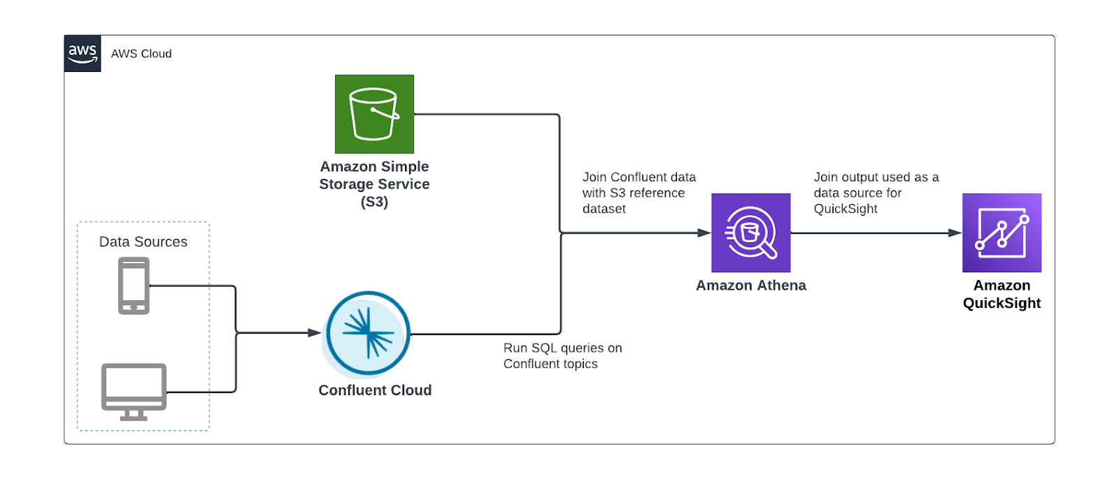
We perform the following steps:
- Register the schema of your Confluent data.
- Configure the Athena connector for Kafka.
- Optionally, interactively analyze Confluent data.
- Create a QuickSight dataset using Athena as the source.
Register the schema
To connect Athena to Confluent, the connector needs the schema of the topic to be registered in the AWS Glue Schema Registry, which Athena uses for query planning.
The following is a sample record in Confluent:
The following is the schema of this record:
The data producer writing the data can register this schema with the AWS Glue Schema Registry. Alternatively, you can use the AWS Management Console or AWS Command Line Interface (AWS CLI) to create a schema manually.
We create the schema manually by running the following CLI command. Replace <registry\_name> with your registry name and make sure that the text in the description field includes the required string {AthenaFederationKafka}:
Next, we run the following command to create a schema inside the newly created schema registry:
Before running the command, be sure to provide the following details:
- Replace <registry\_name> with our AWS Glue Schema Registry name
- Replace <schema\_name> with the name of our Confluent Cloud topic, for example, transactions
- Replace <Compatibility\_Mode> with one of the supported compatibility modes, for example, ‘Backward’
- Replace <Schema> with our schema
Configure and deploy the Athena Connector
With our schema created, we’re ready to deploy the Athena connector. Complete the following steps:
- On the Athena console, choose Data sources in the navigation pane.
- Choose Create data source.
- Search for and select Apache Kafka.

- For Data source name, enter the name for the data source.

This data source name will be referenced in your queries. For example:
Applying this to our use case and previously defined schema, our query would be as follows:
- In the Connection details section, choose Create Lambda function.

You’re redirected to the Applications page on the Lambda console. Some of the application settings are already filled.
The following are the important settings required for integrating with Confluent Cloud. For more information on these settings, refer to Parameters.
- For LambdaFunctionName, enter the name for the Lambda function the connector will use. For example,
athena\_confluent\_connector.
We use this parameter in the next step.
- For KafkaEndpoint, enter the Confluent Cloud bootstrap URL.
You can find this on the Cluster settings page in the Confluent Cloud UI.

Confluent Cloud supports two authentication mechanisms: OAuth and SASL/PLAIN (API keys). The connector doesn’t support OAuth; this leaves us with SASL/PLAIN. SASL/PLAIN uses SSL as a security protocol and PLAIN as SASL mechanism.
- For AuthType, enter
SASL\_SSL\_PLAIN.
The API key and secret used by the connector to access Confluent need to be stored in AWS Secrets Manager.
- Get your Confluent API key or create a new one.
- Run the following AWS CLI command to create the secret in Secrets Manager:
The secret string should have two key-value pairs, one named username and the other password.
- For SecretNamePrefix, enter the secret name prefix created in the previous step.
- If the Confluent cloud cluster is reachable over the internet, leave SecurityGroupIds and SubnetIds blank. Otherwise, your Lambda function needs to run in a VPC that has connectivity to your Confluent Cloud network. Therefore, enter a security group ID and three private subnet IDs in this VPC.
- For SpillBucket, enter the name of an S3 bucket where the connector can spill data.
Athena connectors temporarily store (spill) data to Amazon S3 for further processing by Athena.
- Select I acknowledge that this app creates custom IAM roles and resource policies.
- Choose Deploy.
- Return to the Connection details section on the Athena console and for Lambda, enter the name of the Lambda function you created.
- Choose Next.

- Choose Create data source.
Perform interactive analysis on Confluent data
With the Athena connector set up, our streaming data is now queryable from the same service we use to analyze S3 data lakes. Next, we use Athena to conduct point-in-time analysis of transactions flowing through Confluent Cloud.
Aggregation
We can use standard SQL functions to aggregate the data. For example, we can get the revenue by product category:

Enrich transaction data with customer data
The aggregation example is also available with ksqlDB pull queries. However, Athena’s connector allows us to join the data with other data sources like Amazon S3.
In our use case, the transactions streamed to Confluent Cloud lack detailed information about customers, apart from a customer\_id. However, we have a reference dataset in Amazon S3 that has more information about the customers. With Athena, we can join both datasets together to gain insights about our customers. See the following code:
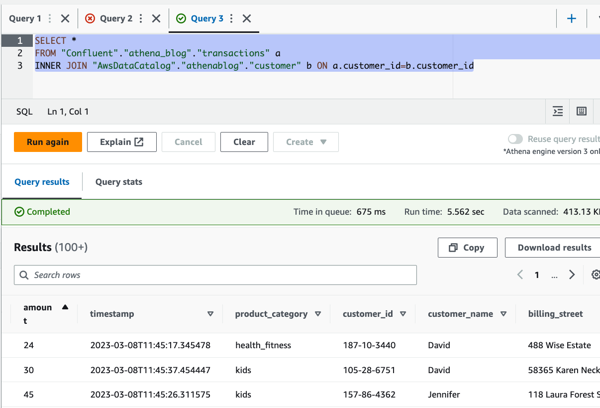
You can see from the results that we were able to enrich the streaming data with customer details, stored in Amazon S3, including name and address.
Visualize data using QuickSight
Another powerful feature this connector brings is the ability to visualize data stored in Confluent using any BI tool that supports Athena as a data source. In this post, we use QuickSight. QuickSight is a machine learning (ML)-powered BI service built for the cloud. You can use it to deliver easy-to-understand insights to the people you work with, wherever they are.
For more information about signing up for QuickSight, see Signing up for an Amazon QuickSight subscription.
Complete the following steps to visualize your streaming data with QuickSight:
- On the QuickSight console, choose Datasets in the navigation pane.
- Choose New dataset.
- Choose Athena as the data source.
- For Data source name, enter a name.
- Choose Create data source.
- In the Choose your table section, choose Use custom SQL.

- Enter the join query like the one given previously, then choose Confirm query.

- Next, choose to import the data into SPICE (Super-fast, Parallel, In-memory Calculation Engine), a fully managed in-memory cache that boosts performance, or directly query the data.
Utilizing SPICE will enhance performance, but the data may need to be periodically updated. You can choose to incrementally refresh your dataset or schedule regular refreshes with SPICE. If you want near-real-time data reflected in your dashboards, select Directly query your data. Note that with the direct query option, user actions in QuickSight, such as applying a drill-down filter, may invoke a new Athena query.
- Choose Visualize.

That’s it, we have successfully connected QuickSight to Confluent through Athena. With just a few clicks, you can create a few visuals displaying data from Confluent.
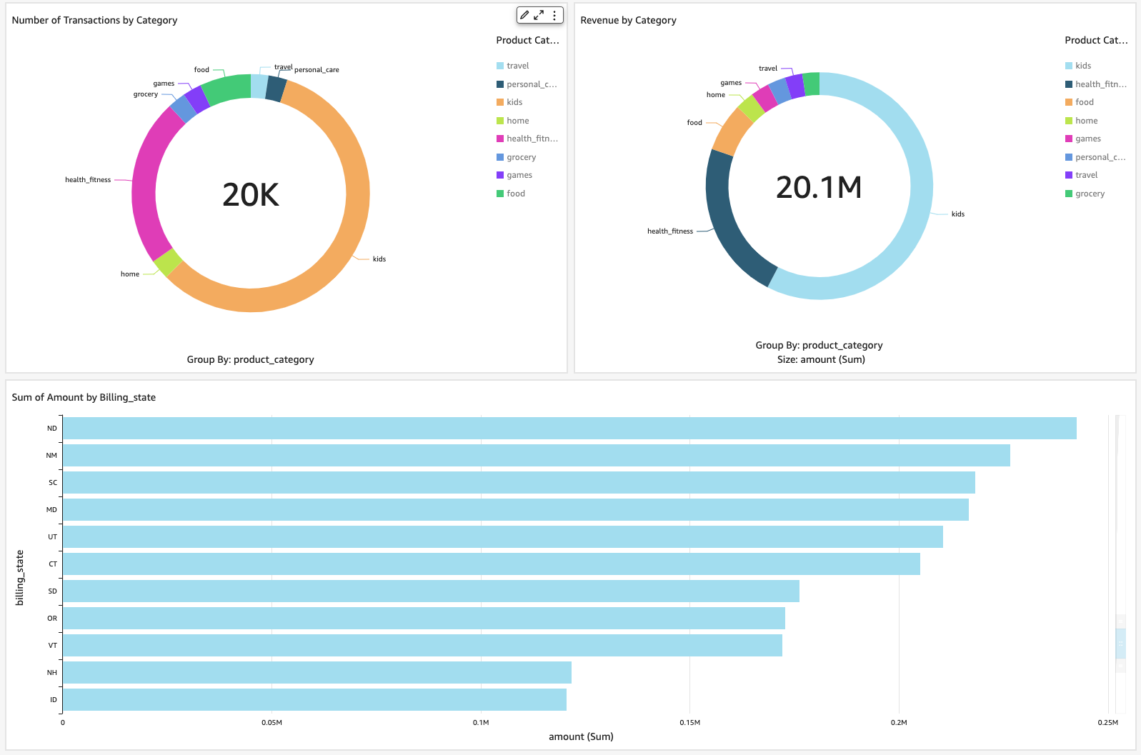
Clean up
To avoid incurring ongoing charges, delete the resources you provisioned by completing the following steps:
- Delete the AWS Glue schema and registry.
- Delete the Athena Kafka connector.
- Delete the QuickSight dataset.
Conclusion
In this post, we discussed use cases for Athena and Confluent. We provided examples of how you can use both for near-real-time data visualization with QuickSight and interactive analysis involving joins between streaming data in Confluent and data stored in Amazon S3.
The Athena connector for Kafka simplifies the process of querying and analyzing streaming data from Confluent Cloud. It removes the need to first move streaming data to persistent storage before it can be used in downstream use cases like business intelligence. This complements the existing integration between Confluent and Athena, using the S3 sink connector, which enables loading streaming data into a data lake, and is an additional option for customers who want to enable interactive analysis on Confluent data.
About the authors
 Ahmed Zamzam is a Senior Partner Solutions Architect at Confluent, with a focus on the AWS partnership. In his role, he works with customers in the EMEA region across various industries to assist them in building applications that leverage their data using Confluent and AWS. Prior to Confluent, Ahmed was a Specialist Solutions Architect for Analytics AWS specialized in data streaming and search. In his free time, Ahmed enjoys traveling, playing tennis, and cycling.
 Geetha Anne is a Partner Solutions Engineer at Confluent with previous experience in implementing solutions for data-driven business problems on the cloud, involving data warehousing and real-time streaming analytics. She fell in love with distributed computing during her undergraduate days and has followed her interest ever since. Geetha provides technical guidance, design advice, and thought leadership to key Confluent customers and partners. She also enjoys teaching complex technical concepts to both tech-savvy and general audiences.
Amazon Redshift Serverless makes it simple to run and scale analytics without having to manage your data warehouse infrastructure. Developers, data scientists, and analysts can work across databases, data warehouses, and data lakes to build reporting and dashboarding applications, perform real-time analytics, share and collaborate on data, and even build and train machine learning (ML) models with Redshift Serverless.
Tags allows you to assign metadata to your AWS resources. You can define your own key and value for your resource tag, so that you can easily manage and filter your resources. Tags can also improve transparency and map costs to specific teams, products, or applications. This way, you can raise cost awareness and also make teams and users accountable for their own cost and usage.
You can now use tagging in Redshift Serverless to categorize the following resources based on your grouping needs:
- Namespace – A collection of database objects and users
- Workgroup – A collection of compute resources
- Snapshot – Point-in-time backups of a cluster
- Recovery point – Recovery points in Redshift Serverless are created every 30 minutes and saved for 24 hours
When using Redshift Serverless, you may have to manage data across many business departments, environments, and billing groups. In doing so, you’re usually faced with one of the following tasks:
- Cost allocation and financial management – You want to know what you’re spending on AWS for a given project, line of business, or environment
- Operations support and incident management – You want to send issues to the right teams and users
- Access control – You want to constrain user access to certain resources
- Security risk management – You want to group resources based on their level of security or data sensitivity and make sure proper controls are in place
In this post, we focus on tagging Redshift Serverless resources for cost allocation and reporting purposes. Knowing where you have incurred costs at the resource, workload, team, and organization level enhances your ability to budget and manage cost.
Solution overview
Let’s say that your company has two departments: marketing and finance. Each department has multiple cost centers and environments, as illustrated in the following figure. In AWS Cost Explorer, you want to create cost reports for Redshift Serverless by department, environment, and cost center.

We start with creating and applying user-defined tags to Amazon Serverless workgroups for respective departments, environments, and cost centers. You can use both the AWS Command Line Interface (AWS CLI) and Redshift Serverless console to tag serverless resources.
The high-level steps are as follows:
- Create tags.
- View and edit tags.
- Set up cost allocation tags.
- Create cost reports.
Create tags
To create tags, complete the following steps:
- On the Amazon Redshift console, choose Manage tags in the navigation pane.

- For Filter by resource type, you can filter by Workgroup, Namespace, Snapshot, and Recovery Point.
- Optionally, you can search for resources by an existing tag by entering values for Tag key or Tag value. For this post, we don’t include any tag filters, so we can view all the resources across our account.

- Select your resource from the search results and choose Manage tags to customize the tag key and value parameters.
Here, you can add new tags, remove tags, save changes, and cancel your changes if needed.
- Because we want to allocate cost across the various departments, we add a new key called
departmentand a new value calledmarketing.
- Choose Save changes.

- Confirm the changes by choosing Apply changes.

For more details on tagging, refer to Tagging resources overview.
View and edit tags
If you already have resources such as workgroups (listed on the Workgroup configuration page) or snapshots (listed on the Data backup page), you can create new tags or edit existing tags on the given resource. In the following example, we manage tags on an existing workgroup.
- On the Amazon Redshift console, choose Workgroup configuration in the navigation pane.
- Select your workgroup and on the Actions menu, choose Manage tags.

Now we can remove existing tags or add new tags. For our use case, let’s assume that the marketing department is no longer using the default workgroup, so we want to remove the current tag.
- Choose Remove next to the marketing tag.

We are given the option to choose Undo if needed.
- Choose Save changes and then Apply the changes to confirm.

After we apply the tags, we can view the full list of resources. The number of tags applied to each resource is found in the Tags column.
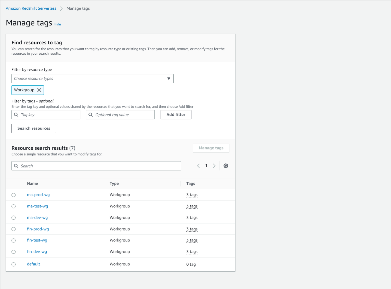
Set up cost allocation tags
After you create and apply the user-defined tags to your Redshift Serverless workgroups, it can take up to 24 hours for the tags to appear on your cost allocation tags page for activation. You can activate tags by using the AWS Billing console for cost allocation tracking with the following steps:
- On the AWS Billing console, choose Cost allocation tags in the navigation pane.
- Under User-defined cost allocation tags¸ select the tags you created and applied (for this example,
cost-center). - Choose Activate.

After we activate all the tags we created, we can view the full list by choosing Active on the drop-down menu.
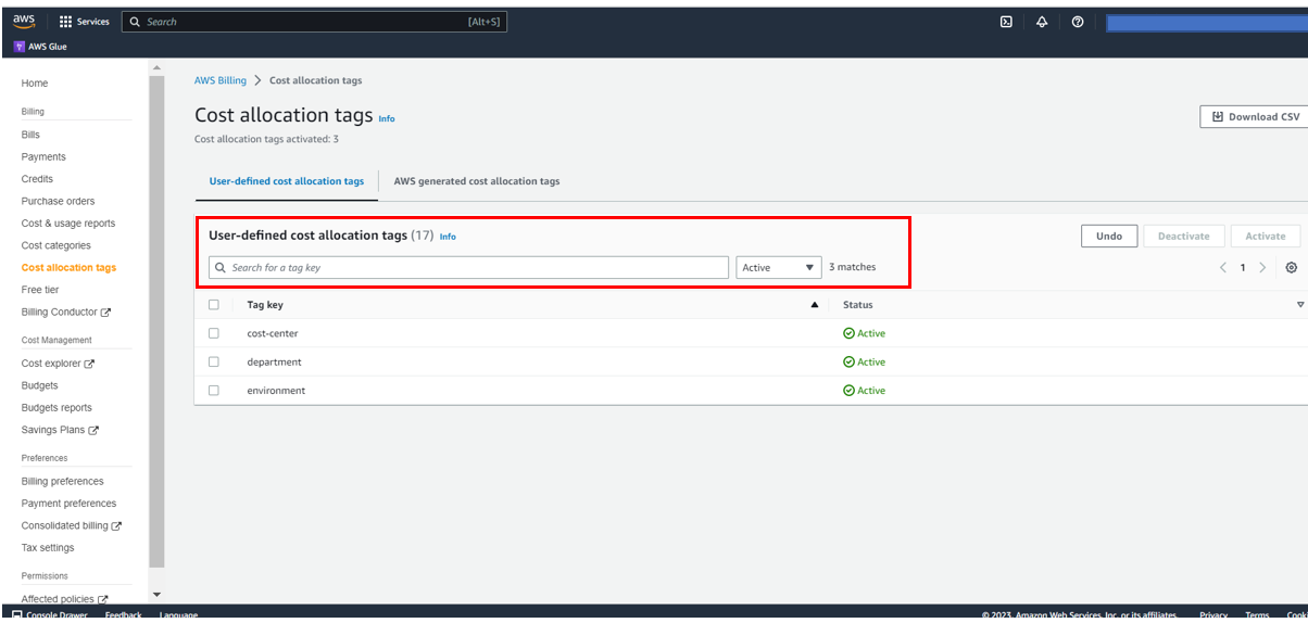
Create cost reports
After you activate the cost allocation tags, they appear on your cost allocation reports in Cost Explorer.
Cost Explorer helps you manage your AWS costs by giving you detailed insights into the line items in your bill. In Cost Explorer, you can visualize daily, monthly, and forecasted spend by combining an array of available filters. Filters allow you to narrow down costs according to AWS service type, linked accounts, and tags.
The following screenshot shows the preconfigured reports in Cost Explorer.

To create custom reports for your cost and usage data, complete the following steps:
- On the AWS Cost Management console, choose Reports in the navigation pane.
- Choose Create new report.
- Select the report type you want to create (for this example, we select Cost and usage).
- Choose Create Report.

- To view weekly Redshift Serverless cost by cost center, choose the applicable settings in the Report parameters pane. For this post, we group data by the cost-center tag and filter data by the department tag.
- Save the report for later use by choosing Save to report library.

- Enter a name for your report, then choose Save report.

The following screenshot shows a sample report for daily Redshift Serverless cost by department.
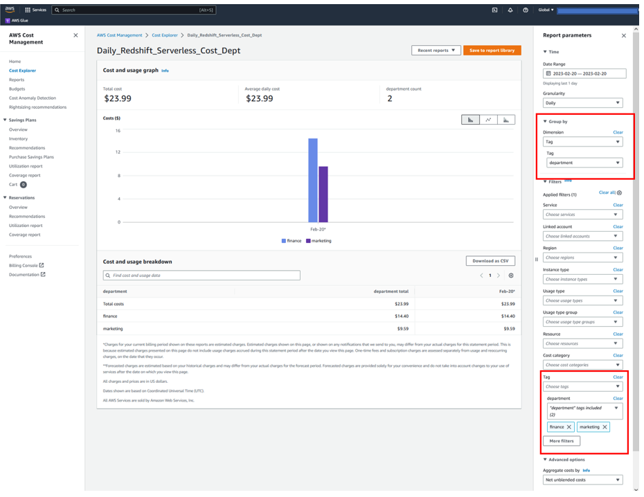
The following screenshot shows an example report of weekly Redshift Serverless cost by environment.
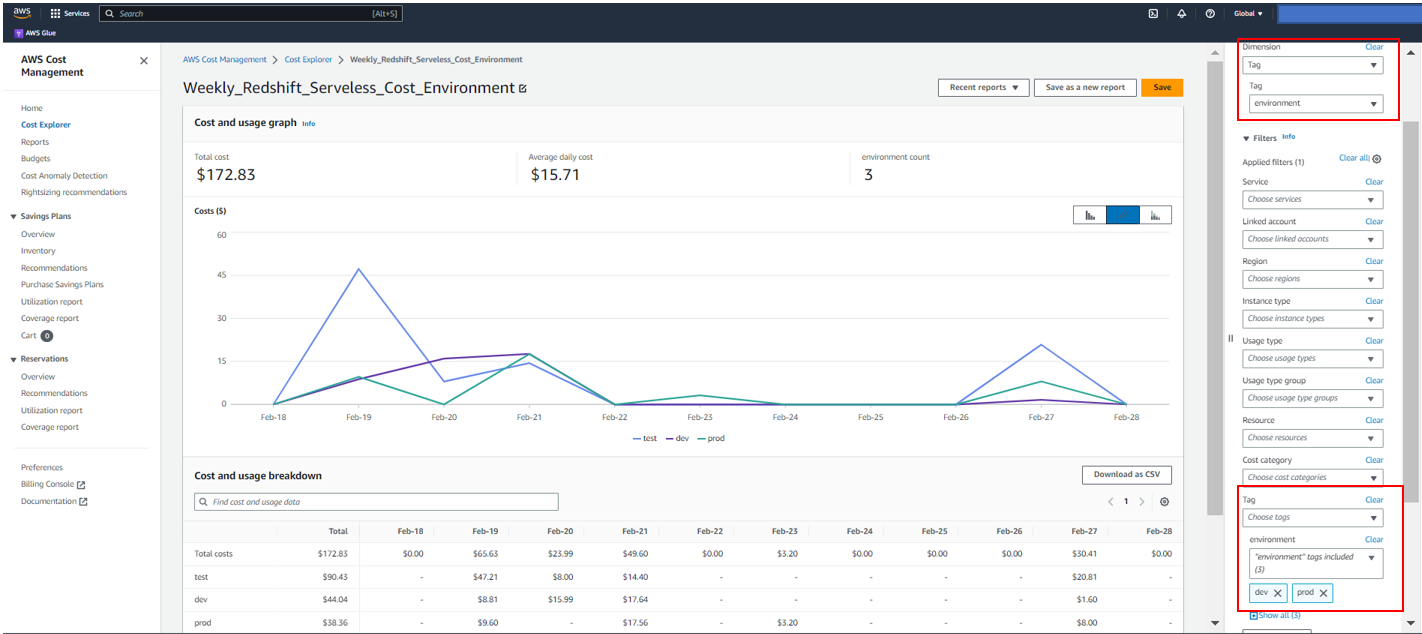
Conclusion
Tagging resources in Amazon Redshift helps you maintain a central place to organize and view resources across the service for billing management. This feature saves you hours of manual work you would spend in grouping your Amazon Redshift resources via a spreadsheet or other manual alternatives.
For more tagging best practices, refer to Tagging AWS resources.
About the Authors
 Sandeep Bajwa is a Sr. Analytics Specialist based out of Northern Virginia, specialized in the design and implementation of analytics and data lake solutions.
 Michael Yitayew is a Product Manager for Amazon Redshift based out of New York. He works with customers and engineering teams to build new features that enable data engineers and data analysts to more easily load data, manage data warehouse resources, and query their data. He has supported AWS customers for over 3 years in both product marketing and product management roles.
We recently announced support for AWS Lake Formation fine-grained access control policies in Amazon Athena queries for data stored in any supported file format using table formats such as Apache Iceberg, Apache Hudi and Apache Hive. AWS Lake Formation allows you to define and enforce database, table, and column-level access policies to query Iceberg tables stored in Amazon S3. Lake Formation provides an authorization and governance layer on data stored in Amazon S3. This capability requires that you upgrade to Athena engine version 3.
Large organizations often have lines of businesses (LoBs) that operate with autonomy in managing their business data. It makes sharing data across LoBs non-trivial. These organizations have adopted a federated model, with each LoB having the autonomy to make decisions on their data. They use the publisher/consumer model with a centralized governance layer that is used to enforce access controls. If you are interested in learning more about data mesh architecture, visit Design a data mesh architecture using AWS Lake Formation and AWS Glue. With Athena engine version 3, customers can use the same fine-grained controls for open data frameworks such as Apache Iceberg, Apache Hudi, and Apache Hive.
In this post, we deep dive into a use-case where you have a producer/consumer model with data sharing enabled to give restricted access to an Apache Iceberg table that the consumer can query. We’ll discuss column filtering to restrict certain rows, filtering to restrict column level access, schema evolution, and time travel.
Solution overview
To illustrate the functionality of fine-grained permissions for Apache Iceberg tables with Athena and Lake Formation, we set up the following components:
- In the producer account:
- An AWS Glue Data Catalog to register the schema of a table in Apache Iceberg format
- Lake Formation to provide fine-grained access to the consumer account
- Athena to verify data from the producer account
- In the consumer account:
- AWS Resource Access Manager (AWS RAM) to create a handshake between the producer Data Catalog and consumer
- Lake Formation to provide fine-grained access to the consumer account
- Athena to verify data from producer account
The following diagram illustrates the architecture.

Prerequisites
Before you get started, make sure you have the following:
- Two AWS accounts, one will act as a producer and other as a consumer
- An understanding of AWS LakeFormation and a user that can act as a Lake Formation admin
- An AWS Identity and Access Management (IAM) role with permissions to create S3 buckets, AWS Glue data catalog, AWS Resource Access Manager, and run SQL queries using Amazon Athena (see Adding and removing IAM identity permissions for reference)
- Any workgroup with Athena engine version 3. For this blog our “primary” workgroup is using Athena engine version 3.
Data producer setup
In this section, we present the steps to set up the data producer.
Create an S3 bucket to store the table data
We create a new S3 bucket to save the data for the table:
- On the Amazon S3 console, create an S3 bucket with unique name (for this post, we use
iceberg-athena-lakeformation-blog). - Create the producer folder inside the bucket to use for the table.

Register the S3 path storing the table using Lake Formation
We register the S3 full path in Lake Formation:
- Navigate to the Lake Formation console.
- If you’re logging in for the first time, you’re prompted to create an admin user.

- In the navigation pane, under Register and ingest, choose Data lake locations.
- Choose Register location, and provide the S3 bucket path that you created earlier.
- Choose
AWSServiceRoleForLakeFormationDataAccessfor IAM role.
For additional information about roles, refer to Requirements for roles used to register locations.
If you enabled encryption of your S3 bucket, you have to provide permissions for Lake Formation to perform encryption and decryption operations. Refer to Registering an encrypted Amazon S3 location for guidance.
- Choose Register location.

Create an Iceberg table using Athena
Now let’s create the table using Athena backed by Apache Iceberg format:
- On the Athena console, choose Query editor in the navigation pane.
- If you’re using Athena for the first time, under Settings, choose Manage and enter the S3 bucket location that you created earlier (
iceberg-athena-lakeformation-blog/producer). - Choose Save.
- In the query editor, enter the following query (replace the location with the S3 bucket that you registered with Lake Formation). Note that we use the default database, but you can use any other database.
- Choose Run.

Share the table with the consumer account
To illustrate functionality, we implement the following scenarios:
- Provide access to selected columns
- Provide access to selected rows based on a filter
Complete the following steps:
- On the Lake Formation console, in the navigation pane under Data catalog, choose Data filters.
- Choose Create new filter.
- For Data filter name, enter
blog\_data\_filter. - For Target database, enter
lf-demo-db. - For Target table, enter
consumer\_iceberg. - For Column-level access, select Include columns.
- Choose the columns to share with the consumer:
country, address, contactfirstname, city, customerid,andcustomername. - For Row filter expression, enter the filter
country='France'. - Choose Create filter.

Now let’s grant access to the consumer account on the consumer\_iceberg table.
- In the navigation pane, choose Tables.
- Select the consumer\_iceberg table, and choose Grant on the Actions menu.

- Select External accounts.
- Enter the external account ID.
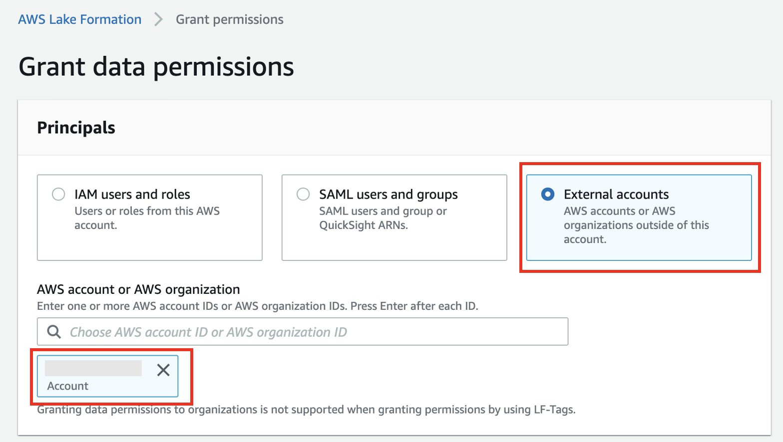
- Select Named data catalog resources.
- Choose your database and table.
- For Data filters, choose the data filter you created.
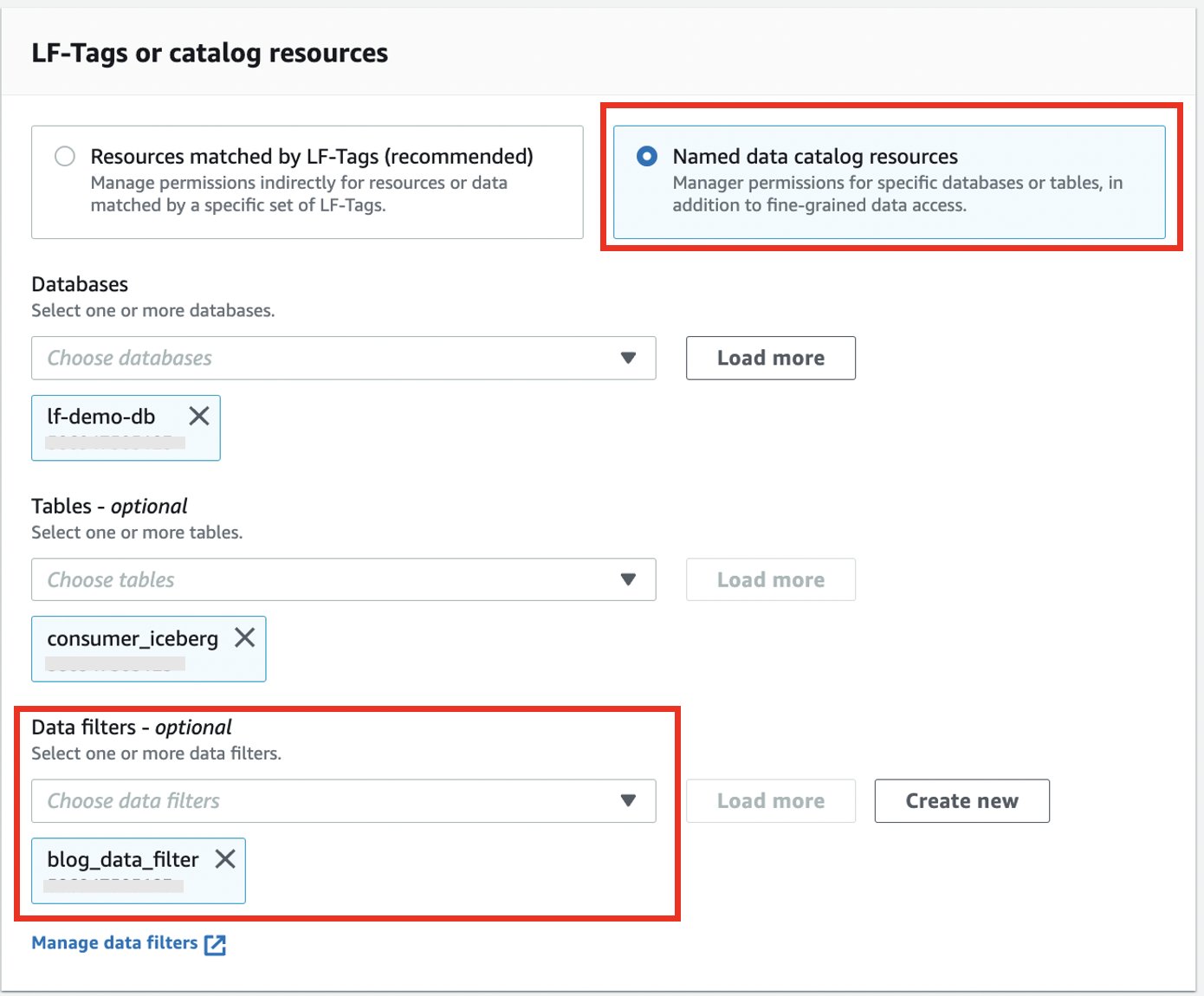
- For Data filter permissions and Grantable permissions, select Select.
- Choose Grant.

Data consumer setup
To set up the data consumer, we accept the resource share and create a table using AWS RAM and Lake Formation. Complete the following steps:
- Log in to the consumer account and navigate to the AWS RAM console.
- Under Shared with me in the navigation pane, choose Resource shares.
- Choose your resource share.

- Choose Accept resource share.
- Note the name of the resource share to use in the next steps.

- Navigate to the Lake Formation console.
- If you’re logging in for the first time, you’re prompted to create an admin user.
- Choose Databases in the navigation pane, then choose your database.
- On the Actions menu, choose Create resource link.

- For Resource link name, enter the name of your resource link (for example,
consumer\_iceberg). - Choose your database and shared table.
- Choose Create.

Validate the solution
Now we can run different operations on the tables to validate the fine-grained access controls.
Insert operation
Let’s insert data into the consumer\_iceberg table in the producer account, and validate the data filtering works as expected in the consumer account.
- Log in to the producer account.
- On the Athena console, choose Query editor in the navigation pane.
- Use the following SQL to write and insert data into the Iceberg table. Use the Query editor to run one query at a time. You can highlight/select one query at a time and click “Run”/“Run again:

- Use the following SQL to read and select data in the Iceberg table:
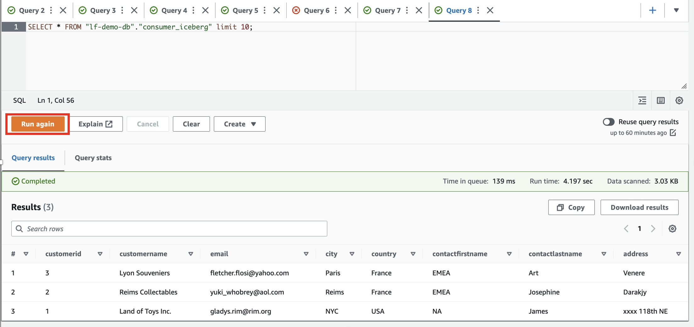
- Log in to the consumer account.
- In the Athena query editor, run the following SELECT query on the shared table:

Based on the filters, the consumer has visibility to a subset of columns, and rows where the country is France.
Update/Delete operations
Now let’s update one of the rows and delete one from the dataset shared with the consumer.
- Log in to the producer account.
- Update
city='Paris' WHERE city='Reims'and delete the rowcustomerid = 3;

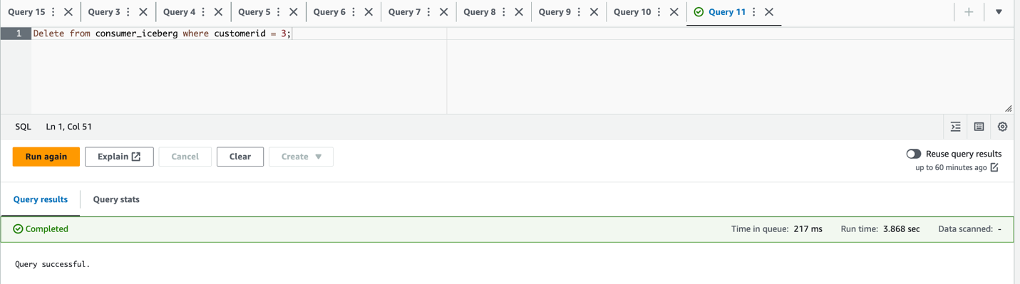
- Verify the updated and deleted dataset:
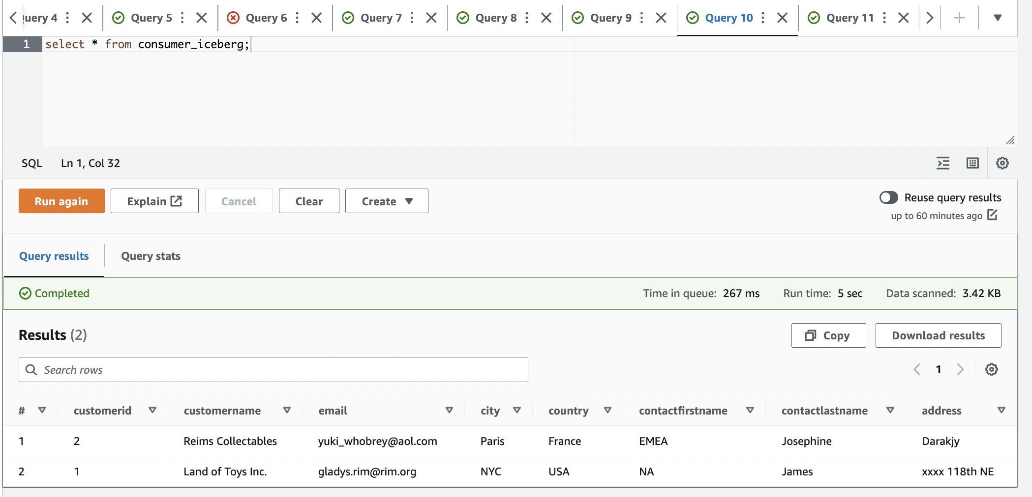
- Log in to the consumer account.
- In the Athena query editor, run the following SELECT query on the shared table:

We can observe that only one row is available and the city is updated to Paris.
Schema evolution: Add a new column
Let’s update one of the rows and delete one from the dataset shared with the consumer.
- Log in to the producer account.
- Add a new column called
geo\_locin the Iceberg table. Use the Query editor to run one query at a time. You can highlight/select one query at a time and click “Run”/“Run again:

To provide visibility to the newly added geo\_loc column, we need to update the Lake Formation data filter.
- On the Lake Formation console, choose Data filters in the navigation pane.
- Select your data filter and choose Edit.

- Under Column-level access, add the new column (
geo\_loc). - Choose Save.

- Log in to the consumer account.
- In the Athena query editor, run the following
SELECTquery on the shared table:
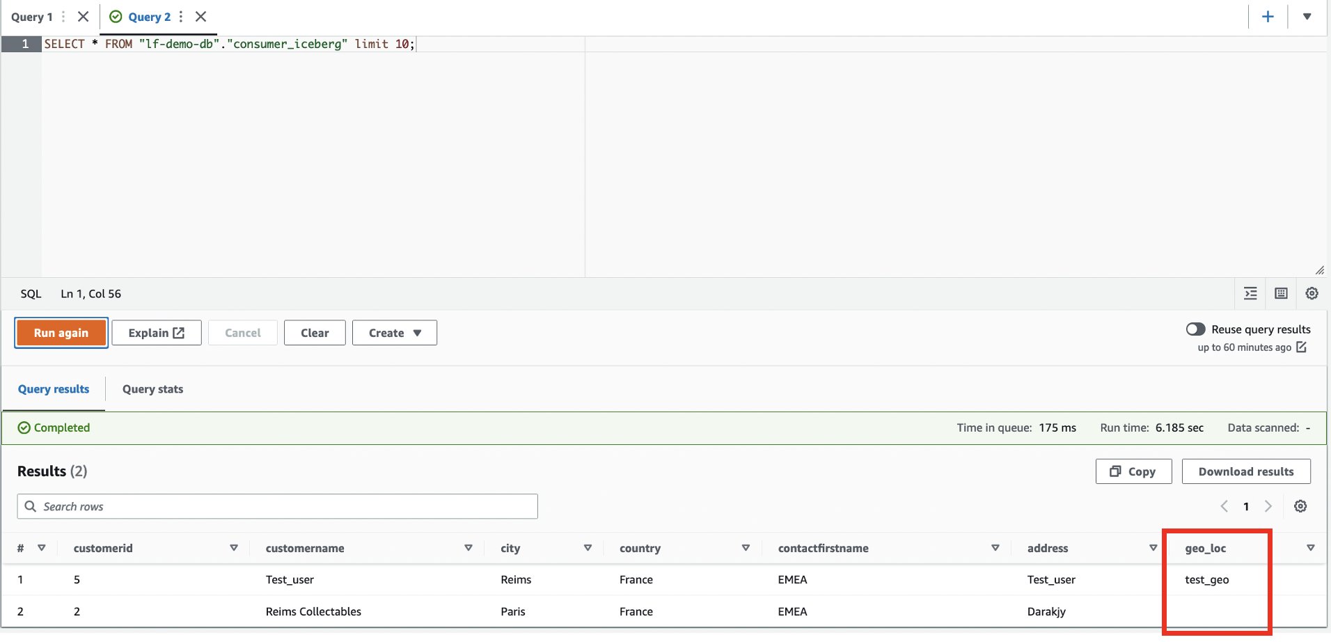
The new column geo\_loc is visible and an additional row.
Schema evolution: Delete column
Let’s update one of the rows and delete one from the dataset shared with the consumer.
- Log in to the producer account.
- Alter the table to drop the address column from the Iceberg table. Use the Query editor to run one query at a time. You can highlight/select one query at a time and click “Run”/“Run again:

We can observe that the column address is not present in the table.
- Log in to the consumer account.
- In the Athena query editor, run the following SELECT query on the shared table:

The column address is not present in the table.
Time travel
We have now changed the Iceberg table multiple times. The Iceberg table keeps track of the snapshots. Complete the following steps to explore the time travel functionality:
- Log in to the producer account.
- Query the system table:
We can observe that we have generated multiple snapshots.
- Note down one of the
committed\_atvalues to use in the next steps (for this example,2023-01-29 21:35:02.176 UTC).

- Use time travel to find the table snapshot. Use the Query editor to run one query at a time. You can highlight/select one query at a time and click “Run”/“Run again:

Clean up
Complete the following steps to avoid incurring future charges:
- On the Amazon S3 console, delete the table storage bucket (for this post, iceberg-athena-lakeformation-blog).
- In the producer account on the Athena console, run the following commands to delete the tables you created:
- In the producer account on the Lake Formation console, revoke permissions to the consumer account.

- Delete the S3 bucket used for the Athena query result location from the consumer account.
Conclusion
With the support for cross account, fine-grained access control policies for formats such as Iceberg, you have the flexibility to work with any format supported by Athena. The ability to perform CRUD operations against the data in your S3 data lake combined with Lake Formation fine-grained access controls for all tables and formats supported by Athena provides opportunities to innovate and simplify your data strategy. We’d love to hear your feedback!
About the authors
 Kishore Dhamodaran is a Senior Solutions Architect at AWS. Kishore helps strategic customers with their cloud enterprise strategy and migration journey, leveraging his years of industry and cloud experience.
 Jack Ye is a software engineer of the Athena Data Lake and Storage team at AWS. He is an Apache Iceberg Committer and PMC member.
 Chris Olson is a Software Development Engineer at AWS.
 Xiaoxuan Li is a Software Development Engineer at AWS.
 Rahul Sonawane is a Principal Analytics Solutions Architect at AWS with AI/ML and Analytics as his area of specialty.
Amazon QuickSight is cloud-native, scalable business intelligence (BI) service that supports identity federation. AWS Identity and Access Management (IAM) allows organizations to use the identities managed in their enterprise identity provider (IdP) and federate single sign-on (SSO) to QuickSight. As more organizations are building centralized user identity stores with all their applications, including on-premises apps, third-party apps, and applications on AWS, they need a solution to automate user provisioning into these applications and keep their attributes in sync with their centralized user identity store.
When architecting a user repository, some organizations decide to organize their users in groups or use attributes (such as department name), or a combination of both. If your organization uses Microsoft Azure Active Directory (Azure AD) for centralized authentication and utilizes its user attributes to organize the users, you can enable federation across all QuickSight accounts as well as manage users and their group membership in QuickSight using events generated in the AWS platform. This allows system administrators to centrally manage user permissions from Azure AD. Provisioning, updating, and de-provisioning users and groups in QuickSight no longer requires management in two places with this solution. This makes sure that users and groups in QuickSight stay consistent with information in Azure AD through automatic synchronization.
In this post, we walk you through the steps required to configure federated SSO between QuickSight and Azure AD via AWS IAM Identity Center (Successor to AWS Single Sign-On) where automatic provisioning is enabled for Azure AD. We also demonstrate automatic user and group membership update using a System for Cross-domain Identity Management (SCIM) event.
Solution overview
The following diagram illustrates the solution architecture and user flow.

In this post, IAM Identity Center provides a central place to bring together administration of users and their access to AWS accounts and cloud applications. Azure AD is the user repository and configured as the external IdP in IAM Identity Center. In this solution, we demonstrate the use of two user attributes (department, jobTitle) specifically in Azure AD. IAM Identity Center supports automatic provisioning (synchronization) of user and group information from Azure AD into IAM Identity Center using the SCIM v2.0 protocol. With this protocol, the attributes from Azure AD are passed along to IAM Identity Center, which inherits the defined attribute for the user’s profile in IAM Identity Center. IAM Identity Center also supports identity federation with SAML (Security Assertion Markup Language) 2.0. This allows IAM Identity Center to authenticate identities using Azure AD. Users can then SSO into applications that support SAML, including QuickSight. The first half of this post focuses on how to configure this end to end (see Sign-In Flow in the diagram).
Next, user information starts to get synchronized between Azure AD and IAM Identity Center via SCIM protocol. You can automate creating a user in QuickSight using an AWS Lambda function triggered by the CreateUser SCIM event originated from IAM Identity Center, which was captured in Amazon EventBridge. In the same Lambda function, you can subsequently update the user’s membership by adding into the specified group (whose name is comprised of two user attributes: department-jobTitle, otherwise create the group if it doesn’t exist yet, prior to adding the membership.
In this post, this automation part is omitted because it would be redundant with the content discussed in the following sections.
This post explores and demonstrates an UpdateUser SCIM event triggered by the user profile update on Azure AD. The event is captured in EventBridge, which invokes a Lambda function to update the group membership in QuickSight (see Update Flow in the diagram). Because a given user is supposed to belong to only one group at a time in this example, the function will replace the user’s current group membership with the new one.
In Part I, you set up SSO to QuickSight from Azure AD via IAM Identity Center (the sign-in flow):
- Configure Azure AD as the external IdP in IAM Identity Center.
- Add and configure an IAM Identity Center application in Azure AD.
- Complete configuration of IAM Identity Center.
- Set up SCIM automatic provisioning on both Azure AD and IAM Identity Center, and confirm in IAM Identity Center.
- Add and configure a QuickSight application in IAM Identity Center.
- Configure a SAML IdP and SAML 2.0 federation IAM role.
- Configure attributes in the QuickSight application.
- Create a user, group, and group membership manually via the AWS Command Line Interface (AWS CLI) or API.
- Verify the configuration by logging in to QuickSight from the IAM Identity Center portal.
In Part II, you set up automation to change group membership upon an SCIM event (the update flow):
- Understand SCIM events and event patterns for EventBridge.
- Create attribute mapping for the group name.
- Create a Lambda function.
- Add an EventBridge rule to trigger the event.
- Verify the configuration by changing the user attribute value at Azure AD.
Prerequisites
For this walkthrough, you should have the following prerequisites:
- IAM Identity Center. For instructions, refer to Steps 1–2 in the AWS IAM Identity Center Getting Started guide.
- A QuickSight account subscription.
- Basic understanding of IAM and privileges required to create an IAM IdP, roles, and policies.
- An Azure AD subscription. You need at least one user with the following attributes to be registered in Azure AD:
- userPrincipalName – Mandatory field for Azure AD user.
- displayName – Mandatory field for Azure AD user.
- Mail – Mandatory field for IAM Identity Center to work with QuickSight.
- jobTitle – Used to allocate user to group
- department – Used to allocate user to group.
- givenName – Optional field.
- surname – Optional field.
Part I: Set up SSO to QuickSight from Azure AD via IAM Identity Center
This section presents the steps to set up the sign-in flow.
Configure an external IdP as Azure AD in IAM Identity Center
To configure your external IdP, complete the following steps:
- On the IAM Identity Center console, choose Settings.
- Choose Actions on the Identity source tab, then choose Change identity source.
- Choose External identity provider, then choose Next.
The IdP metadata is displayed. Keep this browser tab open.
Add and configure an IAM Identity Center application in Azure AD
To set up your IAM Identity Center application, complete the following steps:
- Open a new browser tab.
- Log in to the Azure AD portal using your Azure administrator credentials.
- Under Azure services, choose Azure Active Directory.
- In the navigation pane, under Manage, choose Enterprise applications, then choose New application.
- In the Browse Azure AD Galley section, search for IAM Identity Center, then choose AWS IAM Identity Center (successor to AWS Single Sign-On).

- Enter a name for the application (in this post, we use
IIC-QuickSight) and choose Create. - In the Manage section, choose Single sign-on, then choose SAML.
- In the Assign users and groups section, choose Assign users and groups.
- Choose Add user/group and add at least one user.
- Select User as its role.
- In the Set up single sign on section, choose Get started.
- In the Basic SAML Configuration section, choose Edit, and fill out following parameters and values:
- Identifier – The value in the IAM Identity Center issuer URL field.
- Reply URL – The value in the IAM Identity Center Assertion Consumer Service (ACS) URL field.
- Sign on URL – Leave blank.
- Relay State – Leave blank.
- Logout URL – Leave blank.
- Choose Save.
The configuration should look like the following screenshot.

- In the SAML Certificates section, download the Federation Metadata XML file and the Certificate (Raw) file.

You’re all set with Azure AD SSO configuration at this moment. Later on, you’ll return to this page to configure automated provisioning, so keep this browser tab open.
Complete configuration of IAM Identity Center
Complete your IAM Identity Center configuration with the following steps:
- Go back to the browser tab for IAM Identity Center console which you have kept open in previous step.
- For IdP SAML metadata under the Identity provider metadata section, choose Choose file.
- Choose the previously downloaded metadata file (
IIC-QuickSight.xml). - For IdP certificate under the Identity provider metadata section, choose Choose file.
- Choose the previously downloaded certificate file (
IIC-QuickSight.cer). - Choose Next.
- Enter ACCEPT, then choose Change Identity provider source.
Set up SCIM automatic provisioning on both Azure AD and IAM Identity Center
Your provisioning method is still set as Manual (non-SCIM). In this step, we enable automatic provisioning so that IAM Identity Center becomes aware of the users, which allows identity federation to QuickSight.
- In the Automatic provisioning section, choose Enable.

- Choose Access token to show your token.

- Go back to the browser tab (Azure AD), which you kept open in Step 1.
- In the Manage section, choose Enterprise applications.
- Choose
IIC-QuickSight, then choose Provisioning. - Choose Automatic in Provisioning Mode and enter the following values:
- Tenant URL – The value in the SCIM endpoint field.
- Secret Token – The value in the Access token field.
- Choose Test Connection.
- After the test connection is successfully complete, set Provisioning Status to On.

- Choose Save.
- Choose Start provisioning to start automatic provisioning using the SCIM protocol.
When provisioning is complete, it will result in propagating one or more users from Azure AD to IAM Identity Center. The following screenshot shows the users that were provisioned in IAM Identity Center.

Note that upon this SCIM provisioning, the users in QuickSight should be created using the Lambda function triggered by the event originated from IAM Identity Center. In this post, we create a user and group membership via the AWS CLI (Step 8).
Add and configure a QuickSight application in IAM Identity Center
In this step, we create a QuickSight application in IAM Identity Center. You also configure an IAM SAML provider, role, and policy for the application to work. Complete the following steps:
- On the IAM Identity Center console, on the Applications page, choose Add Application.
- For Pre-integrated application under Select an application, enter
quicksight. - Select Amazon QuickSight, then choose Next.
- Enter a name for Display name, such as
Amazon QuickSight. - Choose Download under IAM Identity Center SAML metadata file and save it in your computer.
- Leave all other fields as they are, and save the configuration.
- Open the application you’ve just created, then choose Assign Users.
The users provisioned via SCIM earlier will be listed.
- Choose all of the users to assign to the application.
Configure a SAML IdP and a SAML 2.0 federation IAM role
To set up your IAM SAML IdP for IAM Identity Center and IAM role, complete the following steps:
- On the IAM console, in the navigation pane, choose Identity providers, then choose Add provider.
- Choose SAML as Provider type, and enter
Azure-IIC-QSas Provider name. - Under Metadata document, choose Choose file and upload the metadata file you downloaded earlier.
- Choose Add provider to save the configuration.
- In the navigation pane, choose Roles, then choose Create role.
- For Trusted entity type, select SAML 2.0 federation.
- For Choose a SAML 2.0 provider, select the SAML provider that you created, then choose Allow programmatic and AWS Management Console access.
- Choose Next.
- On the Add Permission page, choose Next.
In this post, we create QuickSight users via an AWS CLI command, therefore we’re not creating any permission policy. However, if the self-provisioning feature in QuickSight is required, the permission policy for the CreateReader, CreateUser, and CreateAdmin actions (depending on the role of the QuickSight users) is required.
- On the Name, review, and create page, under Role details, enter
qs-reader-azurefor the role. - Choose Create role.
- Note the ARN of the role.
You use the ARN to configure attributes in your IAM Identity Center application.
Configure attributes in the QuickSight application
To associate the IAM SAML IdP and IAM role to the QuickSight application in IAM Identity Center, complete the following steps:
- On the IAM Identity Center console, in the navigation pane, choose Applications.
- Select the
Amazon QuickSightapplication, and on the Actions menu, choose Edit attribute mappings. - Choose Add new attribute mapping.
- Configure the mappings in the following table.
| User attribute in the application | Maps to this string value or user attribute in IAM Identity Center |
| Subject | ${user:email} |
| https://aws.amazon.com/SAML/Attributes/RoleSessionName | ${user:email} |
| https://aws.amazon.com/SAML/Attributes/Role | arn:aws:iam::<ACCOUNTID>:role/qs-reader-azure,arn:aws:iam::<ACCOUNTID>:saml-provider/Azure-IIC-QS |
| https://aws.amazon.com/SAML/Attributes/PrincipalTag:Email | ${user:email} |
Note the following values:
- Replace <ACCOUNTID> with your AWS account ID.
PrincipalTag:Emailis for the email syncing feature for self-provisioning users that need to be enabled on the QuickSight admin page. In this post, don’t enable this feature because we register the user with an AWS CLI command.
- Choose Save changes.
Create a user, group, and group membership with the AWS CLI
As described earlier, users and groups in QuickSight are being created manually in this solution. We create them via the following AWS CLI commands.
The first step is to create a user in QuickSight specifying the IAM role created earlier and email address registered in Azure AD. The second step is to create a group with the group name as combined attribute values from Azure AD for the user created in the first step. The third step is to add the user into the group created earlier; member-name indicates the user name created in QuickSight that is comprised of <IAM Role name>/<session name>. See the following code:
At this point, the end-to-end configuration of Azure AD, IAM Identity Center, IAM, and QuickSight is complete.
Verify the configuration by logging in to QuickSight from the IAM Identity Center portal
Now you’re ready to log in to QuickSight using the IdP-initiated SSO flow:
- Open a new private window in your browser.
- Log in to the IAM Identity Center portal (
https://d-xxxxxxxxxx.awsapps.com/start).
You’re redirected to the Azure AD login prompt.
- Enter your Azure AD credentials.
You’re redirected back to the IAM Identity Center portal.
- In the IAM Identity Center portal, choose Amazon QuickSight.

You’re automatically redirected to your QuickSight home.

Part II: Automate group membership change upon SCIM events
In this section, we configure the update flow.
Understand the SCIM event and event pattern for EventBridge
When an Azure AD administrator makes any changes to the attributes on the particular user profile, the change will be synced with the user profile in IAM Identity Center via SCIM protocol, and the activity is recorded in an AWS CloudTrail event called UpdateUser by sso-directory.amazonaws.com (IAM Identity Center) as the event source. Similarly, the CreateUser event is recorded when a user is created on Azure AD, and the DisableUser event is for when a user is disabled.
The following screenshot on the Event history page shows two CreateUser events: one is recorded by IAM Identity Center, and the other one is by QuickSight. In this post, we use the one from IAM Identity Center.

In order for EventBridge to be able to handle the flow properly, each event must specify the fields of an event that you want the event pattern to match. The following event pattern is an example of the UpdateUser event generated in IAM Identity Center upon SCIM synchronization:
In this post, we demonstrate an automatic update of group membership in QuickSight that is triggered by the UpdateUser SCIM event.
Create attribute mapping for the group name
In order for the Lambda function to manage group membership in QuickSight, it must obtain the two user attributes (department and jobTitle). To make the process simpler, we’re combining two attributes in Azure AD (department, jobTitle) into one attribute in IAM Identity Center (title), using the attribute mappings feature in Azure AD. IAM Identity Center then uses the title attribute as a designated group name for this user.
- Log in to the Azure AD console, navigate to Enterprise Applications,
IIC-QuickSight, and Provisioning. - Choose Edit attribute mappings.
- Under Mappings, choose Provision Azure Active Directory Users.

- Choose
jobTitlefrom the list of Azure Active Directory Attributes. - Change the following settings:
- Mapping Type –
Expression - Expression –
Join("-", [department], [jobTitle]) - Target attribute –
title

- Mapping Type –
- Choose Save.
- You can leave the provisioning page.
The attribute is automatically updated in IAM Identity Center. The updated user profile looks like the following screenshots (Azure AD on the left, IAM Identity Center on the right).


Create a Lambda function
Now we create a Lambda function to update QuickSight group membership upon the SCIM event. The core part of the function is to obtain the user’s title attribute value in IAM Identity Center based on the triggered event information, and then to ensure that the user exists in QuickSight. If the group name doesn’t exist yet, it creates the group in QuickSight and then adds the user into the group. Complete the following steps:
- On the Lambda console, choose Create function.
- For Name, enter
UpdateQuickSightUserUponSCIMEvent. - For Runtime, choose Python 3.9.
- For Time Out, set to 15 seconds.
- For Permissions, create and attach an IAM role that includes the following permissions (the trusted entity (principal) should be
lambda.amazonaws.com): - Write Python code using the Boto3 SDK for IdentityStore and QuickSight. The following is the entire sample Python code:
Note that this Lambda function requires Boto3 1.24.64 or later. If the Boto3 included in the Lambda runtime is older than this, use a Lambda layer to use the latest version of Boto3. For more details, refer to How do I resolve “unknown service”, “parameter validation failed”, and “object has no attribute” errors from a Python (Boto 3) Lambda function.
Add an EventBridge rule to trigger the event
To create an EventBridge rule to invoke the previously created Lambda function, complete the following steps:
- On the EventBridge console, create a new rule.
- For Name, enter
updateQuickSightUponSCIMEvent. - For Event pattern, enter the following code:
- For Targets, choose the Lambda function you created (
UpdateQuickSightUserUponSCIMEvent). - Enable the rule.
Verify the configuration by changing a user attribute value at Azure AD
Let’s modify a user’s attribute at Azure AD, and then check if the new group is created and that the user is added into the new one.
- Go back to the Azure AD console.
- From Manage, click Users.
- Choose one of the users you previously used to log in to QuickSight from the IAM Identity Center portal.
- Choose Edit properties, then edit the values for Job title and Department.

- Save the configuration.
- From Manage, choose Enterprise application, your application name, and Provisioning.
- Choose Stop provisioning and then Start provisioning in sequence.
In Azure AD, the SCIM provisioning interval is fixed to 40 minutes. To get immediate results, we manually stop and start the provisioning.

- Navigate to the QuickSight console.
- On the drop-down user name menu, choose Manage QuickSight.
- Choose Manage groups.
Now you should find that the new group is created and the user is assigned to this group.

Clean up
When you’re finished with the solution, clean up your environment to minimize cost impact. You may want to delete the following resources:
- Lambda function
- Lambda layer
- IAM role for the Lambda function
- CloudWatch log group for the Lambda function
- EventBridge rule
- QuickSight account
- Note : There can only be one QuickSight account per AWS account. So your QuickSight account might already be used by other users in your organization. Delete the QuickSight account only if you explicitly set it up to follow this blog and are absolutely sure that it is not being used by any other users.
- IAM Identity Center instance
- IAM ID Provider configuration for Azure AD
- Azure AD instance
Summary
This post provided step-by-step instructions to configure IAM Identity Center SCIM provisioning and SAML 2.0 federation from Azure AD for centralized management of QuickSight users. We also demonstrated automated group membership updates in QuickSight based on user attributes in Azure AD, by using SCIM events generated in IAM Identity Center and setting up automation with EventBridge and Lambda.
With this event-driven approach to provision users and groups in QuickSight, system administrators can have full flexibility in where the various different ways of user management could be expected depending on the organization. It also ensures the consistency of users and groups between QuickSight and Azure AD whenever a user accesses QuickSight.
We are looking forward to hearing any questions or feedback.
About the authors
 Takeshi Nakatani is a Principal Bigdata Consultant on Professional Services team in Tokyo. He has 25 years of experience in IT industry, expertised in architecting data infrastructure. On his days off, he can be a rock drummer or a motorcyclyst.
 Wakana Vilquin-Sakashita is Specialist Solution Architect for Amazon QuickSight. She works closely with customers to help making sense of the data through visualization. Previously Wakana worked for S&P Global assisting customers to access data, insights and researches relevant for their business.
AWS Payments is part of the AWS Commerce Platform (CP) organization that owns the customer experience of paying AWS invoices. It helps AWS customers manage their payment methods and payment preferences, and helps customers make self-service payments to AWS.
The Machine Learning, Data and Analytics (MLDA) team at AWS Payments enables data-driven decision-making across payments processes and partners by delivering data, business insights, and causal and ML inferences through a scalable set of data, insights, and ML inference services.
In this post, we discuss how to democratize data access to Amazon Redshift using the Amazon Redshift Query Editor V2 .
Background
At AWS Payments, we had been using Redash to allow our users to author and run SQL queries against our Amazon Redshift data warehouse. Redash is a web-based SQL client application that can be used to author and run queries, visualize query results with charts, and collaborate with teams.
Over time, we began to notice incompatibilities between Redash’s operations and the needs of our workload.
We had the following requirements in mind when looking for an alternative tool:
- Authentication and authorization
- Provide data access without creating a database user and password
- Allow list users using permission groups (POSIX/LDAP) for accessing the tool
- Limit user access to database objects
- User experience
- Run SQL queries on the selected database
- Save a query and rerun it later
- Write a dynamic SQL query and run the query based on input parameters
- Export a query result to CSV
- Search saved queries
- Share a query with other users as a URL
After an evaluation of alternate services, we chose the Amazon Redshift Query Editor V2.
Amazon Redshift Query Editor V2
The Amazon Redshift Query Editor V2 has the following benefits:
- It makes data across analytics and data scientists more accessible with a unified web-based analyst workbench for data analysts to explore, share, and collaborate on data through a SQL interface
- It provides a managed service that allows you to focus on exploring your data without managing your infrastructure
- Users can log in to the Query Editor using single sign-on (SSO)
- Users can connect to Amazon Redshift using federated access without providing a user name and password
- It enables you to collaborate with team members by providing the ability to share saved queries securely
- You can benefit from new features as soon as they get released by the Amazon Redshift Query Editor team
- You can keep track of changes made to saved queries using the Query History feature
- You can write parameterized SQL queries, which allows you to reuse a query with different values
- You can turn on the Chart feature to display a graphic visualization of the current page of results
- You can use notebooks to organize, annotate, and share multiple SQL queries in a single document
- You can run multiple queries in parallel by running each query in a separate tab
However, it presented the following challenges:
- To restrict user access to other AWS services within our AWS account, we attached the AWS Identity and Access Management (IAM) policies (see the appendix at the end of this post) to the SAML IAM role. The policies promote the following:
- The user can only access the Query Editor V2 service.
- The federated user gets assigned to a database group with limited access.
- The Query Editor V2 currently doesn’t support cross-account Amazon Redshift connections. However, we set up Amazon Redshift data sharing to access the Amazon Redshift cluster from other AWS accounts. For more details, refer to Sharing data across clusters in Amazon Redshift.
Architecture overview
The following diagram illustrates our architecture.

In the following sections, we will walk you through the steps to set up the query editor and migrate Redash queries.
Prerequisites
To implement this solution, you must set up federated access to the Amazon Redshift Query Editor V2 using your identity provider (IdP) services.
You can find more information in the following posts:
- Federate access to Amazon Redshift query editor V2 with Active Directory Federation Services
- Federate single sign-on access to Amazon Redshift query editor v2 with Okta
Set up Amazon Redshift Query Editor V2
To set up the query editor, complete the following steps:
- Create an Amazon Redshift database group with read-only access.
- Create an IAM role for accessing Query Editor V2 in an AWS account and attach the required IAM policies based on your use case. For more information, refer to Configuring your AWS account.
- Create a trust relationship between your IdP and AWS.

- Add the principal tag
sqlworkbench-teamto the IAM role to share queries. For more information, refer to Sharing a query.

Migrate Redash queries to Amazon Redshift Query Editor V2
In this section, we walk you through different ways to migrate your Redash queries to the Amazon Redshift Query Editor V2.
Query without parameters
Querying without parameters is pretty straightforward, just copy your query from Redash and enter it in the query editor.
- In Redash, navigate to the saved query and choose Edit Source.
- Copy the source query.
- In Amazon RedShift Query Editor V2, enter the query into the editor, choose the Save icon, and give your query a title.
Query with parameters
In Redash, a string between {{ }} will be treated as a parameter, but Amazon RedShift Query Editor V2 uses ${ } to identify a parameter. To migrate queries with parameters, follow the same steps but replace {{ with ${ and }} with }.
The following screenshot shows an example query in Redash.
 The following screenshot shows the same query in Amazon RedShift Query Editor V2.

Multi-part query to a Query Editor V2 notebook
For a multi-part query, copy the query of each section of a Redash dashboard and add it to a notebook. The notebook in Amazon Redshift Query Editor V2 runs queries successively. You also can add a description for your query.
The following screenshot shows an example query on the Redash dashboard.

The following screenshot shows the query in an Amazon Redshift Query Editor V2 notebook.

Summary
In this post, we demonstrated how we set up Amazon Redshift Query Editor V2 with SSO and Amazon Redshift federated access, and migrated our customers from Redash to Amazon Redshift Query Editor V2. This solution reduced our operational cost of maintaining a third-party application and its infrastructure.
If you have similar use cases and need to provide a web-based tool to your customers to explore data on your Amazon Redshift cluster, consider using Amazon Redshift Query Editor V2.
Appendix: Customer IAM policies
In this section, we provide the code for the IAM policies we attached to the SAML IAM role to restrict user access to other AWS services within our AWS account:
- query-editor-credentials-policy – In the following code, provide your Region, account, and cluster parameters to grant access to Amazon Redshift to get cluster credentials, create users, and allow users to join groups:
- query-editor-access-policy – See the following code:
- query-editor-notebook-policy – See the following code:
About the Authors

Mohammad Nejad leads the AWS Payments Data Platform team. He has experience leading teams, architecting designs, implementing solutions, and launching products. Currently, his team focuses on building a modern data platform on AWS to provide a complete solution for processing, analyzing, and presenting data.
Erol Murtezaoglu, a Technical Product Manager at AWS, is an inquisitive and enthusiastic thinker with a drive for self-improvement and learning. He has a strong and proven technical background in software development and architecture, balanced with a drive to deliver commercially successful products. Erol highly values the process of understanding customer needs and problems, in order to deliver solutions that exceed expectations.
Mohamed Shaaban is a Senior Software Engineer in Amazon Redshift and is based in Berlin, Germany. He has over 12 years of experience in the software engineering. He is passionate about cloud services and building solutions that delight customers. Outside of work, he is an amateur photographer who loves to explore and capture unique moments.
This post was co-written by Mahesh Pasupuleti and Gaurav Shah from Poshmark.
Poshmark is a leading social marketplace for new and secondhand styles for women, men, kids, pets, home, and more. By combining the human connection of physical shopping with the scale, ease, and selection benefits of Ecommerce, Poshmark makes buying and selling simple, social, and sustainable. Its community of more than 80 million registered users across the US, Canada, Australia, and India is driving a more sustainable future for the fashion industry.
An important goal to achieve for any organization is to grow the top line revenue. Top line revenue refers to the total value of sales of an organization’s services or products. The two main approaches organizations employ to increase revenue are to expand geographically to enter new markets and to increase market share within a market by improving customer experience (CX).
Improving CX is a well-known guideline to attract and retain customers and thereby increase the market share. In this post, we share how Poshmark improved CX and accelerated revenue growth by using a real-time analytics solution. We discuss how to create such a solution using Amazon Kinesis Data Streams, Amazon Managed Streaming for Kafka (Amazon MSK), Amazon Kinesis Data Analytics for Apache Flink; the design decisions that went into the architecture; and the observed business benefits by Poshmark.
High-level challenge: The need for real-time analytics
Previous efforts at Poshmark for improving CX through analytics were based on batch processing of analytics data and using it on a daily basis to improve CX. Although these batch analytics-based efforts were successful to some extent, they saw opportunities to improve the customer experience with real-time personalization and security guidance during the customer’s interaction with the Poshmark app. The customer insights gathered from the batch analytics couldn’t be paired with the current customer activities in real time due to the latencies involved in enriching the current activities with the knowledge gained through batch processes. Therefore, the opportunity to provide tailored offers or showcase products based on customers’ preference and behaviors in near-real time, which contributes to a much better customer experience, was missing. Similarly, the opportunity to catch fraud within a second, before checkout, was also missing.
To improve the customer experience, Poshmark decided to invest in building a real-time analytics platform to enable real-time capabilities, as explained further in this post. Poshmark engineers worked closely with AWS architects through the AWS Data Lab program. The AWS Data Lab offers accelerated, joint engineering engagements between customers and AWS technical resources to create tangible deliverables that accelerate data and analytics modernization initiatives. The Design Lab is one half to two day engagement with customer team offering prescriptive guidance to arrive at the optimal solution architecture design before you embark on building the platform.
Designing the solution architecture through the AWS Data Lab process
The business and technical stakeholders from Poshmark and the AWS Data Lab architects discussed near-to-long-term business requirements along with the functional and non-functional capabilities required to decide on the architecture approach. They reviewed the current state architecture and constraints to understand data flow and technical integration points. The joint team discussed the pros and cons of various AWS services that already exist in Poshmark’s current architecture, as well as other AWS services that can meet the requirements.
Poshmark wanted to address the following business use cases via the real-time analytics platform:
- Sessionization – Poshmark captures both server-side application events and client-side tracking events. They wanted to use these events to identify and analyze user sessions to track behavior.
- Illegitimate sign-up and sign-in prevention – Poshmark wanted to detect and ban illegitimate sign-up or sign-in events from bots or non-human traffic in real time on the Poshmark application.
- IP translation – The IP addresses present in events will be translated to city, state, and zip, and enriched with other information to implement near-real-time, location-aware services encompassing security-related functions as well as personalization functions.
- Anonymization – Poshmark wanted to anonymize events and make the data available for internal users for querying in near-real time.
- Personalized recommendations – User behavior based on clickstream events can be captured up to the last second before enriching it for personalization and sending it to the model to predict the recommendations.
- Other use cases – Additional use cases relating to aggregations and machine learning (ML) inference use cases such as authorization to operate, listing spam detection, and avoiding account takeovers (ATOs), among others.
One common pattern identified for these use cases was the need for a central data enrichment pipeline to enrich incoming raw events before event data can be utilized for actual business processing. In the Design Lab, we focused on design for data enrichment pipelines aimed at enriching events with data from static files, dynamic data stores such as databases, APIs, or within the same event stream for the aforementioned streaming use cases. Later in this post, we cover the salient points discussed during the lab around design and architecture.
Batch analytics solution architecture
The following diagram shows the previous architecture at Poshmark. For brevity, only the flow pertaining to the real-time analytics platform is explained.

User interactions on Poshmark web and mobile applications generate server-side events. These events include add to cart, orders, transactions, and more on application servers, and the page view, clicks, and more on tracking servers. Fluentd with an Amazon Kinesis plugin is set up on both the application and tracking servers to send these events to Amazon Kinesis Data Streams. The Fluentd Kinesis plugin aggregates events before sending to Kinesis Data Streams. A single Kinesis data stream is currently set up to capture these events. A random partition key is configured in Fluentd for the events to allow even distribution of events across shards. The event data format is nested JSON. Poshmark maintains the same schema grammar at the first level of JSON for both server-side and client-side server events. The attributes at nested level can differ between server-side and client-side events.
Poshmark receives around 1 billion events per day (100 million per hour during peak hours, 10 million per hour during non-peak hours). The average size of the event record is 1.2 KB.
The data from the Kinesis data stream is consumed by two applications:
- A Spark streaming application on Amazon EMR is used to write data from the Kinesis data stream to a data lake hosted on Amazon Simple Storage Service (Amazon S3) in a partitioned way. The data from the S3 data lake is used for batch processing and analytics through Amazon EMR and Amazon Redshift.
- Druid hosted on Amazon Elastic Compute Cloud (Amazon EC2) integrates with the Kinesis data stream for streaming ingestion and allows users to run slice-and-dice OLAP queries. Operational dashboards are hosted on Grafana integrated with Druid.
Desired enhancements to the initial solution
The use cases discussed during the architecture sessions fall into one or more combinations of the following stream processing requirements:
- Stateless event processing – For example, near-real-time anonymization.
- External lookup – Looking up a value from external stores. For example, IP address, city, zip, state, or ID.
- Stateful data processing – Accessing past events or aggregations or ML inferences.
To meet these requirements, the streaming platform is divided into two layers:
- Central data enrichment – This layer runs enrichments commonly required by downstream streaming applications. This will help avoid replication of the same enrichment logic in each application and enable better operational maintenance. The enrichment should strive for per-record processing in most cases.
- Specific streaming applications – This layer will house specific streaming applications with respect to use cases and utilize enriched data from the central data enrichment pipeline.
For central data enrichment, we made the following enhancements to the platform:
- The total latency including ingestion and data enrichment was super critical and should be in the range of double-digit millisecond latency based on the overall latency budget of Poshmark to achieve real-time ML responses to events. The absolute lowest ingestion latency was achieved by Kafka, and the team decided to go with the managed version of Kafka, Amazon MSK.
- Similarly, low-latency processing of data is also required, and appropriate framework should be considered accordingly.
- Exactly-once delivery guarantees were required to avoid data duplication resulting in wrong calculations.
- The enrichment source could be any source such as static files, databases, and APIs and latencies can vary between them. A number of server-side and client-side events are generated when a user interacts with a Poshmark application. As a result, the same information from the enrichment source is required to enrich each event. This frequently accessed information cached in a centralized cache will optimize fetch time.
Design decisions for the new solution
Poshmark made the following design decisions for central data enrichment:
- Kafka can support double-digit millisecond latency from producer to consumer with appropriate performance tuning. Kafka can provide exactly-once semantics both at producers and consumer applications. AWS provides Kafka as part of its Amazon MSK offering, eliminating the operational overhead of maintaining and running Kafka cluster infrastructure on AWS, thereby allowing you to focus on developing and running Kafka-based applications. Poshmark decided to use Amazon MSK for their streaming ingestion and storage requirements.
- We also decided to use Flink for streaming data enrichment applications for the following reasons:
- Flink can provide low-latency processing even at higher throughput with exactly-once guarantees. Spark Structured Streaming on the other hand can provide low latency with low throughput due to microbatch-based processing. Spark Structured Streaming continuous processing is an experimental feature and provides at-least once guarantees.
- The enrichment requests call to an external store if modeled in a map function (Spark’s map API or Flink’s MapFunction API) will make synchronous calls to the external store. The call will wait for a response from the external store before processing the next event, adding to delays and reducing overall throughput. The asynchronous interaction will allow sending requests and receiving responses concurrently from external stores. This will reduce wait time and improve overall throughput. Flink supports async I/O operators natively, allowing users to use asynchronous request clients with data streams. The API handles the integration with data streams, well as handling order, event time, fault tolerance, and more. Spark Structured Streaming doesn’t provide any such support natively and leaves it to users for custom implementation.

- Poshmark selected Kinesis Data Analytics for Apache Flink to run the data enrichment application. Kinesis Data Analytics for Apache Flink provides the underlying infrastructure for your Apache Flink applications. It handles core capabilities like provisioning compute resources, parallel computation, automatic scaling, and application backups (implemented as checkpoints and snapshots).
- An enrichment microservice accompanying Amazon ElastiCache for Redis was set up to abstract access from data enrichment applications. The AsyncFunction in the Flink async I/O operator isn’t multi-threaded and won’t work in a truly asynchronous way if the call is blocked or waiting for a response. The enrichment microservice handles requests and responses asynchronously coming from Flink async I/O operators. The data is also cached in ElastiCache for Redis to improve the latency of the microservice.
- The Poshmark ML applications are the consumers of this enriched data. The team has built and deployed different ML models over time. These models include a learning to rank algorithm, fraud detection, personalization and recommendations, and online spam filtering. Previously, for deploying each model into production, the Poshmark team had to go through a series of infrastructure setup steps that involved data extraction from real-time sources, building real-time aggregate features from streaming data, storing these features in a low-latency database (Redis) for sub-millisecond inferences, and finally performing inferences via Amazon SageMaker hosted endpoints.
- We also designed an ML feature storage pipeline that consumes data from the enriched streaming sources (Kinesis or Kafka), generate single-level and aggregated-level features, and ingest these generated features into a feature store repository with a very low latency of less than 80 milliseconds.
- The ML models are now able to extract the needed features with latency less than 10 milliseconds from the feature repository and perform real-time model inferencing.
Real-time analytics solution architecture
The following diagram illustrates the solution architecture for real-time analytics with Amazon MSK and Kinesis Data Analytics for Apache Flink.

The workflow is as follows:
- Users interact on Poshmark’s web or mobile application.
- Server-side events are captured on application servers and client-side events are captured on tracking servers. These events are written in the downstream MSK cluster.
- The raw events will be ingested into the MSK cluster using the Fluentd plugin to produce data for Kafka.
- The enrichment microservice consists of reactive (asynchronous) enrichment lookup APIs fetching data from persistent data stores. ElastiCache for Redis caches frequently accessed data, reducing fetch time for enrichment lookup APIs.
- The Flink application running on Kinesis Data Analytics for Apache Flink consumes raw events from Amazon MSK and runs data enrichment on a per-record basis. The Flink data enrichment application uses Flink’s async I/O to read external data from the enrichment lookup store for enriching stream events.
- Enriched events are written in the MSK cluster under different enriched events topics.
- The existing Spark streaming application consumes from the enriched events topic (or raw events topic) in Amazon MSK and writes the data into an S3 data lake.
- Druid streaming ingestion now reads from the enriched events topic or raw events topic in Amazon MSK depending on the requirements.
Enrichment of the captured event data
In this section, we discuss the different steps to enrich the captured event data.
Enrichment processing
Kinesis Data Analytics for Apache Flink provides the underlying infrastructure for the Apache Flink applications. It handles core capabilities like provisioning compute resources, parallel computation, automatic scaling, and application backups (implemented as checkpoints and snapshots). You can use the high-level Flink programming features (such as operators, functions, sources, and sinks) in the same way that you use them when hosting the Flink infrastructure yourself.
Flink on Amazon EMR gives the flexibility to choose your Flink version, installation, configuration, instances, and storage. However, you also have to take care of cluster management and operational requirements such as scaling, application backup, and provisioning.
Enrichment lookup store
The AsyncFunction in the Flink async I/O operator isn’t multi-threaded and won’t work in a truly asynchronous way if the call is blocked or waiting for a response. The enrichment lookup API should handle requests and responses asynchronously coming from Flink async I/O operators. The enrichment lookup API can be hosted on Amazon EC2 or containers such as Amazon Elastic Container Service (Amazon ECS) or Amazon Elastic Kubernetes Service (Amazon EKS).
A number of server-side and client-side events are generated when a user interacts with a Poshmark application. As a result, the same information is required to enrich each event. This frequently accessed information cached in a centralized cache can optimize fetch time. The latency to the centralized cache can be further reduced by hosting the client (enrichment lookup API) and cache server in the same Availability Zone.
Reconciliation in case of pipeline errors
The event enrichment can fail in data enrichment applications for various reasons, such as the external store timing out or missing information in the store. The enriched fields may or may not be critical for downstream streaming applications. You should build your downstream streaming applications considering that these failures can occur and implement a fallback mechanism, for example retrying on-demand enrichment from the application. The failure handling will also be governed by latency tolerance of the application.
The processing of data is based on event time. In some situations, data can arrive late in the platform. Both Flink and Spark allow lateness and watermarks for users to handle late-arriving data by defining thresholds. Late-arriving data beyond the threshold is discarded from processing. It’s possible to get this discarded too-late data in Flink using a side output. There is no such provision in Spark Structured Streaming.
A few streaming applications require their batch counterpart to reconcile data hourly or daily to handle data mismatch or data discrepancy due to late-arriving data or missing data.
Improved customer experience
The new real-time architecture offered the following benefits for an improved customer experience:
- Anonymization – Poshmark is now able to provide and utilize real-time anonymized data for multiple functions both internally and externally because anonymization happens in real time.
- Fraud mitigation – Poshmark was previously able to detect and prevent 45% of ATOs with the batch-based solution. With the real-time system, Poshmark is able to prevent 80% of ATOs.
- Personalization – By providing personalized search results, Poshmark achieved an 8% improvement on clickthrough rates for search. This is a significant increase in the top of the funnel, increasing overall search conversions.
Improvement in these three factors helped end-customers gain confidence in the Poshmark app and website, which in turn enabled customers to increase their interaction with the app and helped accelerate customer engagement and growth.
Conclusion
In this post, we discussed the ingestion of real-time clickstream and log event data into Amazon MSK. We showed how enrichment of the captured data can be performed through Kinesis Data Analytics for Apache Flink. We broke up the enrichment processing into multiple components, such as Kinesis Data Analytics for Apache Flink, the enrichment microservices and the enrichment lookup store, and an enrichment cache. We discussed the downstream applications that used this enriched customer information to perform real-time security checks and offer personalized recommendations to end-users. We also discussed some of the areas that may need attention in case there are failures in the pipeline. Lastly, we showed how Poshmark improved their customer experience and gained market share by implementing this real-time analytics pipeline.
About the authors
 Mahesh Pasupuleti is a VP of Data & Machine Learning Engineering at Poshmark. He has helped several startups succeed in different domains, including media streaming, healthcare, the financial sector, and marketplaces. He loves software engineering, building high performance teams, and strategy, and enjoys gardening and playing badminton in his free time.
 Gaurav Shah is Director of Data Engineering and ML at Poshmark. He and his team help build data-driven solutions to drive growth at Poshmark.
 Raghu Mannam is a Sr. Solutions Architect at AWS in San Francisco. He works closely with late-stage startups, many of which have had recent IPOs. His focus is end-to-end solutioning including security, DevOps automation, resilience, analytics, machine learning, and workload optimization in the cloud.
 Deepesh Malviya is Solutions Architect Manager on the AWS Data Lab team. He and his team help customers architect and build data, analytics, and machine learning solutions to accelerate their key initiatives as part of the AWS Data Lab.
In the first post of this series, we described how AWS Glue for Apache Spark works with Apache Hudi, Linux Foundation Delta Lake, and Apache Iceberg datasets tables using the native support of those data lake formats. This native support simplifies reading and writing your data for these data lake frameworks so you can more easily build and maintain your data lakes in a transactionally consistent manner. This feature removes the need to install a separate connector and reduces the configuration steps required to use these frameworks in AWS Glue for Apache Spark jobs.
These data lake frameworks help you store data more efficiently and enable applications to access your data faster. Unlike simpler data file formats such as Apache Parquet, CSV, and JSON, which can store big data, data lake frameworks organize distributed big data files into tabular structures that enable basic constructs of databases on data lakes.
Expanding on the functionality we announced at AWS re:Invent 2022, AWS Glue now natively supports Hudi, Delta Lake and Iceberg through the AWS Glue Studio visual editor. If you prefer authoring AWS Glue for Apache Spark jobs using a visual tool, you can now choose any of these three data lake frameworks as a source or target through a graphical user interface (GUI) without any custom code.
Even without prior experience using Hudi, Delta Lake or Iceberg, you can easily achieve typical use cases. In this post, we demonstrate how to ingest data stored in Hudi using the AWS Glue Studio visual editor.
Example scenario
To demonstrate the visual editor experience, this post introduces the Global Historical Climatology Network Daily (GHCN-D) dataset. The data is publicly accessible through an Amazon Simple Storage Service (Amazon S3) bucket. For more information, see the Registry of Open Data on AWS. You can also learn more in Visualize over 200 years of global climate data using Amazon Athena and Amazon QuickSight.
The Amazon S3 location s3://noaa-ghcn-pds/csv/by\_year/ has all the observations from 1763 to the present organized in CSV files, one file for each year. The following block shows an example of what the records look like:
The records have fields including ID, DATE, ELEMENT, and more. Each combination of ID, DATE, and ELEMENT represents a unique record in this dataset. For example, the record with ID as AE000041196, ELEMENT as TAVG, and DATE as 20220101 is unique.
In this tutorial, we assume that the files are updated with new records every day, and want to store only the latest record per the primary key (ID and ELEMENT) to make the latest snapshot data queryable. One typical approach is to do an INSERT for all the historical data, and calculate the latest records in queries; however, this can introduce additional overhead in all the queries. When you want to analyze only the latest records, it’s better to do an UPSERT (update and insert) based on the primary key and DATE field rather than just an INSERT in order to avoid duplicates and maintain a single updated row of data.
Prerequisites
To continue this tutorial, you need to create the following AWS resources in advance:
- An AWS Identity and Access Management (IAM) role for your ETL job or notebook as instructed in Set up IAM permissions for AWS Glue Studio
- An S3 bucket for storing data
- An AWS Glue database called
hudi\_native
Process a Hudi dataset on the AWS Glue Studio visual editor
Let’s author an AWS Glue job to read daily records in 2022, and write the latest snapshot into the Hudi table on your S3 bucket using UPSERT. Complete following steps:
- Open AWS Glue Studio.
- Choose Jobs.
- Choose Visual with a source and target.
- For Source and Target, choose Amazon S3, then choose Create.
A new visual job configuration appears. The next step is to configure the data source to read an example dataset:
- Under Visual, choose Data source – S3 bucket.
- Under Node properties, for S3 source type, select S3 location.
- For S3 URL, enter
s3://noaa-ghcn-pds/csv/by\_year/2022.csv.
The data source is configured.

The next step is to configure the data target to ingest data in Apache Hudi on your S3 bucket:
- Choose Data target – S3 bucket.
- Under Data target properties- S3, for Format, choose Apache Hudi.
- For Hudi Table Name, enter
ghcn. - For Hudi Storage Type, choose Copy on write.
- For Hudi Write Operation, choose Upsert.
- For Hudi Record Key Fields, choose
ID. - For Hudi Precombine Key Field, choose
DATE. - For Compression Type, choose GZIP.
- For S3 Target location, enter
s3://<Your S3 bucket name>/<Your S3 bucket prefix>/hudi\_native/ghcn/. (Provide your S3 bucket name and prefix.)
To make it easy to discover the sample data, and also make it queryable from Athena, configure the job to create a table definition on the AWS Glue Data Catalog:
- For Data Catalog update options, select Create a table in the Data Catalog and on subsequent runs, update the schema and add new partitions.
- For Database, choose
hudi\_native. - For Table name, enter
ghcn. - For Partition keys – optional, choose
ELEMENT.
Now your data integration job is authored in the visual editor completely. Let’s add one remaining setting about the IAM role, then run the job:
- Under Job details, for IAM Role, choose your IAM role.
- Choose Save, then choose Run.

- Navigate to the Runs tab to track the job progress and wait for it to complete.

Query the table with Athena
Now that the job has successfully created the Hudi table, you can query the table through different engines, including Amazon Athena, Amazon EMR, and Amazon Redshift Spectrum, in addition to AWS Glue for Apache Spark.
To query through Athena, complete the following steps:
- On the Athena console, open the query editor.
- In the query editor, enter the following SQL and choose Run:
SELECT * FROM "hudi\_native"."ghcn" limit 10;The following screenshot shows the query result.

Let’s dive deep into the table to understand how the data is ingested and focus on the records with ID=’AE000041196′.
- Run the following query to focus on the very specific example records with
ID='AE000041196':
SELECT * FROM "hudi\_native"."ghcn" WHERE ID='AE000041196';The following screenshot shows the query result.

The original source file 2022.csv has historical records for record ID='USW00012894' from 20220101 to 20221231, however the query result shows only four records, one record per ELEMENT at the latest snapshot of the day 20221230 or 20221231. Because we used the UPSERT write option when writing data, we configured the ID field as a Hudi record key field, the DATE field as a Hudi precombine field, and the ELEMENT field as partition key field. When two records have the same key value, Hudi picks the one with the largest value for the precombine field. When the job ingested data, it compared all the values in the DATE field for each pair of ID and ELEMENT, and then picked the record with the largest value in the DATE field.
According to the preceding result, we were able to ingest the latest snapshot from all the 2022 data. Now let’s do an UPSERT of the new 2023 data to overwrite the records on the target Hudi table.
- Go back to AWS Glue Studio console, modify the source S3 location to
s3://noaa-ghcn-pds/csv/by\_year/2023.csv, then save and run the job.

- Run the same Athena query from the Athena console.

Now you see that the four records have been updated with the new records in 2023.
If you have further future records, this approach works well to upsert new records based on the Hudi record key and Hudi precombine key.
Clean up
Now to the final step, cleaning up the resources:
- Delete the AWS Glue database
hudi\_native. - Delete the AWS Glue table
ghcn. - Delete the S3 objects under
s3://<Your S3 bucket name>/<Your S3 bucket prefix>/hudi\_native/ghcn2022/.
Conclusion
This post demonstrated how to process Hudi datasets using the AWS Glue Studio visual editor. The AWS Glue Studio visual editor enables you to author jobs while taking advantage of data lake formats and without needing expertise in them. If you have comments or feedback, please feel free to leave them in the comments.
About the authors
Noritaka Sekiyama is a Principal Big Data Architect on the AWS Glue team. He is responsible for building software artifacts to help customers. In his spare time, he enjoys cycling with his new road bike.
 Scott Long is a Front End Engineer on the AWS Glue team. He is responsible for implementing new features in AWS Glue Studio. In his spare time, he enjoys socializing with friends and participating in various outdoor activities.
Sean Ma is a Principal Product Manager on the AWS Glue team. He has an 18+ year track record of innovating and delivering enterprise products that unlock the power of data for users. Outside of work, Sean enjoys scuba diving and college football.
Amazon Athena is a serverless and interactive query service that allows you to easily analyze data in Amazon Simple Storage Service (Amazon S3) and 25-plus data sources, including on-premises data sources or other cloud systems using SQL or Python. Athena built-in capabilities include querying for geospatial data; for example, you can count the number of earthquakes in each Californian county. One disadvantage of analyzing at county-level is that it may give you a misleading impression of which parts of California have had the most earthquakes. This is because the counties aren’t equally sized; a county may have had more earthquakes simply because it’s a big county. What if we wanted a hierarchical system that allowed us to zoom in and out to aggregate data over different equally-sized geographic areas?
In this post, we present a solution that uses Uber’s Hexagonal Hierarchical Spatial Index (H3) to divide the globe into equally-sized hexagons. We then use an Athena user-defined function (UDF) to determine which hexagon each historical earthquake occurred in. Because the hexagons are equally-sized, this analysis gives a fair impression of where earthquakes tend to occur.
At the end, we’ll produce a visualization like the one below that shows the number of historical earthquakes in different areas of the western US.
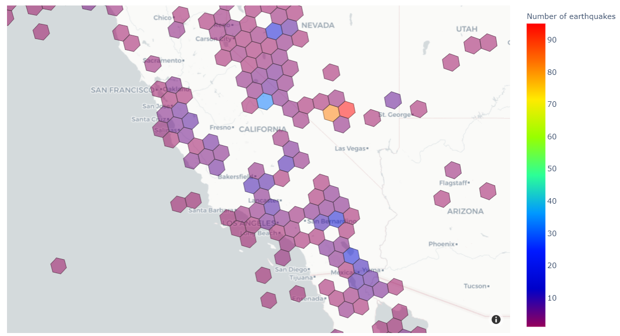
H3 divides the globe into equal-sized regular hexagons. The number of hexagons depends on the chosen resolution, which may vary from 0 (122 hexagons, each with edge lengths of about 1,100 km) to 15 (569,707,381,193,162 hexagons, each with edge lengths of about 50 cm). H3 enables analysis at the area level, and each area has the same size and shape.
Solution overview
The solution extends Athena’s built-in geospatial capabilities by creating a UDF powered by AWS Lambda. Finally, we use an Amazon SageMaker notebook to run Athena queries that are rendered as a choropleth map. The following diagram illustrates this architecture.
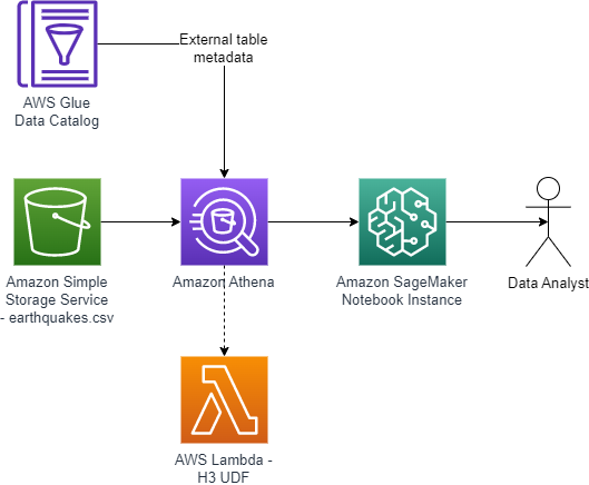
The end-to-end architecture is as follows:
- A CSV file of historical earthquakes is uploaded into an S3 bucket.
- An AWS Glue external table is created based on the earthquake CSV.
- A Lambda function calculates H3 hexagons for parameters (latitude, longitude, resolution). The function is written in Java and can be called as a UDF using queries in Athena.
- A SageMaker notebook uses an AWS SDK for pandas package to run a SQL query in Athena, including the UDF.
- A Plotly Express package renders a choropleth map of the number of earthquakes in each hexagon.
Prerequisites
For this post, we use Athena to read data in Amazon S3 using the table defined in the AWS Glue Data Catalog associated with our earthquake dataset. In terms of permissions, there are two main requirements:
- Athena has access to the S3 bucket where you store the earthquake data and another S3 bucket used to store the output of Athena queries.
- The AWS Identity and Access Management (IAM) role or user you use to run this example is authorized to use Athena. For details, see AWS managed policies for Amazon Athena.
Configure Amazon S3
The first step is to create an S3 bucket to store the earthquake dataset, as follows:
- Download the CSV file of historical earthquakes from GitHub.
- On the Amazon S3 console, choose Buckets in the navigation pane.
- Choose Create bucket.
- For Bucket name, enter a globally unique name for your data bucket.
- Choose Create folder, and enter the folder name
earthquakes. - Upload the file to the S3 bucket. In this example, we upload the
earthquakes.csvfile to theearthquakesprefix.
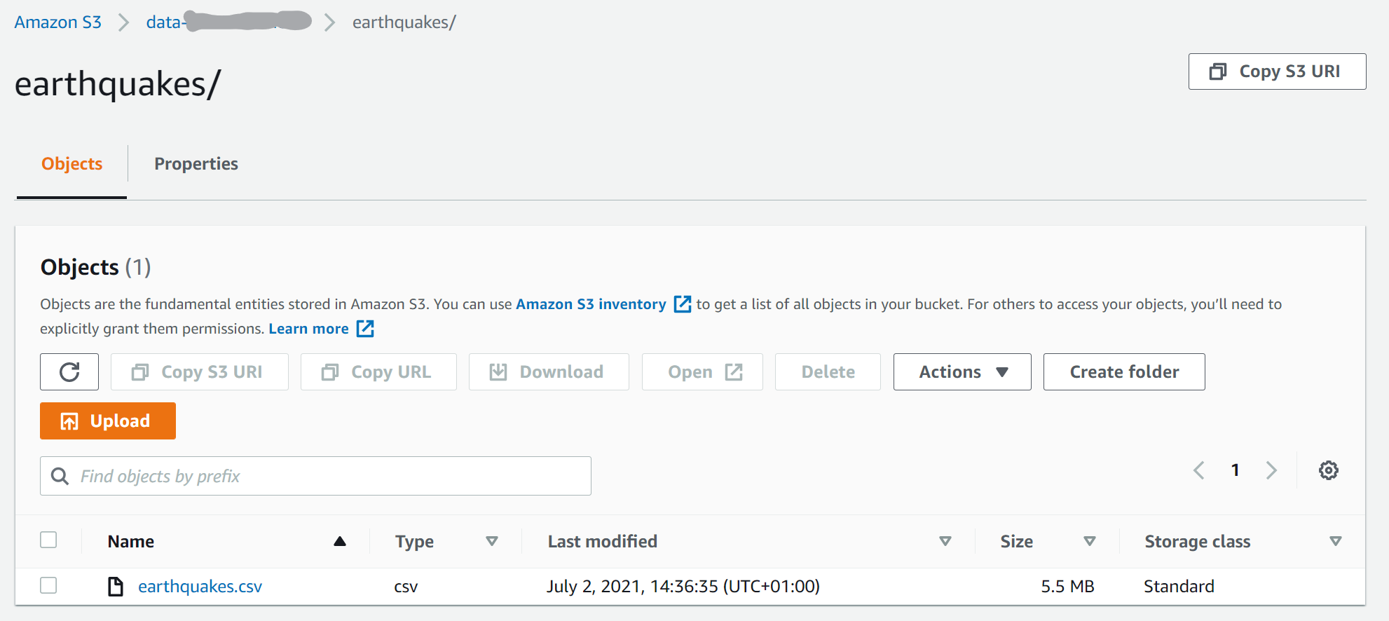
Create a table in Athena
Navigate to Athena console to create a table. Complete the following steps:
- On the Athena console, choose Query editor.
- Select your preferred Workgroup using the drop-down menu.

- In the SQL editor, use the following code to create a table in the default database:
Create a Lambda function for the Athena UDF
For a thorough explanation on how to build Athena UDFs, see Querying with user defined functions. We use Java 11 and Uber H3 Java binding to build the H3 UDF. We provide the implementation of the UDF on GitHub.
There are several options for deploying a UDF using Lambda. In this example, we use the AWS Management Console. For production deployments, you probably want to use infrastructure as code such as the AWS Cloud Development Kit (AWS CDK). For information about how to use the AWS CDK to deploy the Lambda function, refer to the project code repository. Another possible deployment option is using AWS Serverless Application Repository (SAR).
Deploy the UDF
Deploy the Uber H3 binding UDF using the console as follows:
- Go to binary directory in the GitHub repository, and download
aws-h3-athena-udf-*.jarto your local desktop. - Create a Lambda function called
H3UDFwith Runtime set to Java 11 (Corretto), and Architecture set to x86\_64.

- Upload the
aws-h3-athena-udf*.jarfile.

- Change the handler name to
com.aws.athena.udf.h3.H3AthenaHandler.

- In the General configuration section, choose Edit to set the memory of the Lambda function to 4096 MB, which is an amount of memory that works for our examples. You may need to set the memory size larger for your use cases.

Use the Lambda function as an Athena UDF
After you create the Lambda function, you’re ready to use it as a UDF. The following screenshot shows the function details.
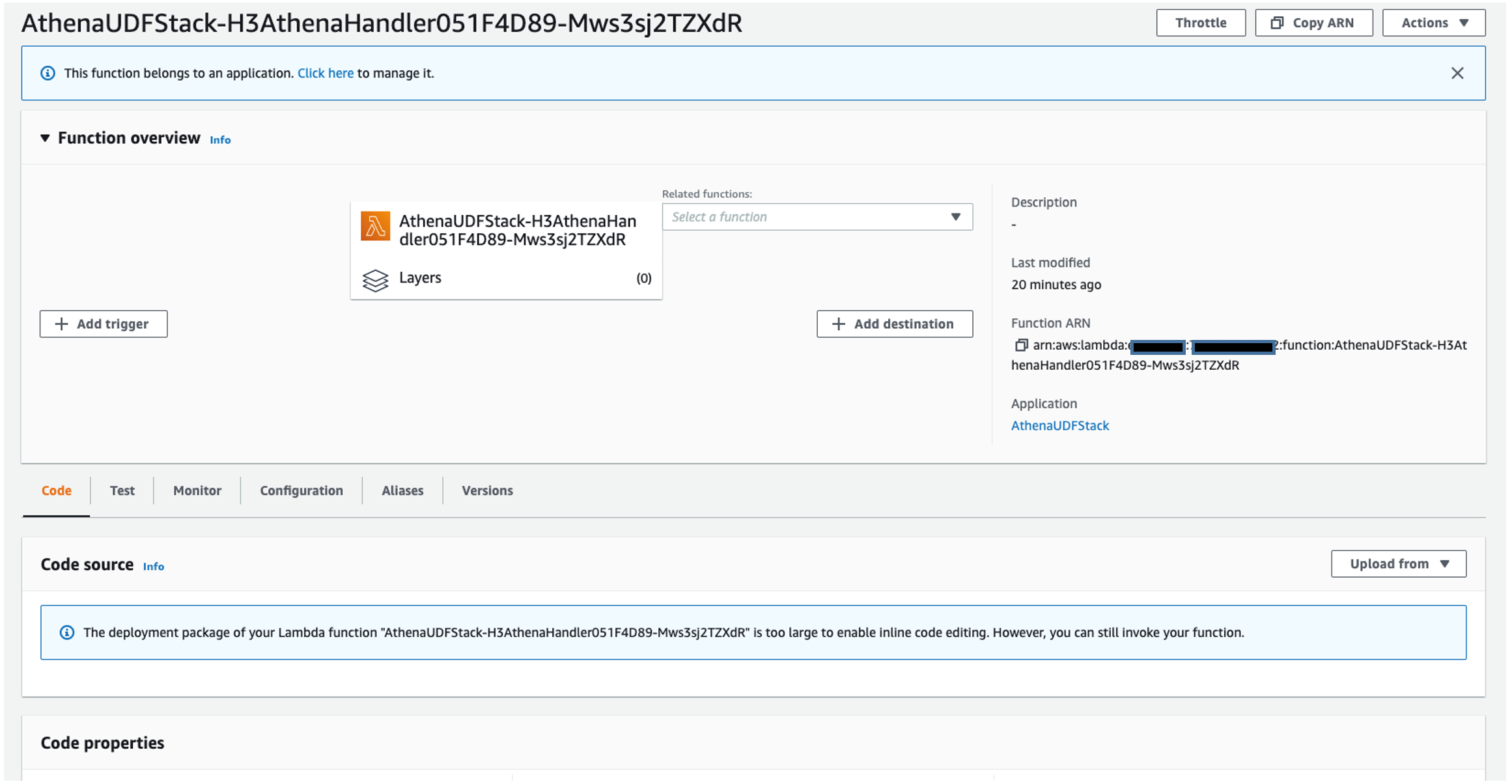
You can now use the function as an Athena UDF. On the Athena console, run the following command:

The udf/examples folder in the GitHub repository includes more examples of the Athena queries.
Developing the UDFs
Now that we showed you how to deploy a UDF for Athena using Lambda, let’s dive deeper into how to develop these kinds of UDFs. As explained in Querying with user defined functions, in order to develop a UDF, we first need to implement a class that inherits UserDefinedFunctionHandler. Then we need to implement the functions inside the class that can be used as UDFs of Athena.
We begin the UDF implementation by defining a class H3AthenaHandler that inherits the UserDefinedFunctionHandler. Then we implement functions that act as wrappers of functions defined in the Uber H3 Java binding. We make sure that all the functions defined in the H3 Java binding API are mapped, so that they can be used in Athena as UDFs. For example, we map the lat\_lng\_to\_cell\_address function used in the preceding example to the latLngToCell of the H3 Java binding.
On top of the call to the Java binding, many of the functions in the H3AthenaHandler check whether the input parameter is null. The null check is useful because we don’t assume the input to be non-null. In practice, null values for an H3 index or address are not unusual.
The following code shows the implementation of the get\_resolution function:
Some H3 API functions such as cellToLatLng return List<Double> of two elements, where the first element is the latitude and the second is longitude. The H3 UDF that we implement provides a function that returns well-known text (WKT) representation. For example, we provide cell\_to\_lat\_lng\_wkt, which returns a Point WKT string instead of List<Double>. We can then use the output of cell\_to\_lat\_lng\_wkt in combination with the built-in spatial Athena function ST\_GeometryFromText as follows:
Athena UDF only supports scalar data types and does not support nested types. However, some H3 APIs return nested types. For example, the polygonToCells function in H3 takes a List<List<List<GeoCoord>>>. Our implementation of polygon\_to\_cells UDF receives a Polygon WKT instead. The following shows an example Athena query using this UDF:
Use SageMaker notebooks for visualization
A SageMaker notebook is a managed machine learning compute instance that runs a Jupyter notebook application. In this example, we will use a SageMaker notebook to write and run our code to visualize our results, but if your use case includes Apache Spark then using Amazon Athena for Apache Spark would be a great choice. For advice on security best practices for SageMaker, see Building secure machine learning environments with Amazon SageMaker. You can create your own SageMaker notebook by following these instructions:
- On the SageMaker console, choose Notebook in the navigation pane.
- Choose Notebook instances.
- Choose Create notebook instance.
- Enter a name for the notebook instance.
- Choose an existing IAM role or create a role that allows you to run SageMaker and grants access to Amazon S3 and Athena.
- Choose Create notebook instance.

- Wait for the notebook status to change from
CreatingtoInService. - Open the notebook instance by choosing Jupyter or JupyterLab.
Explore the data
We’re now ready to explore the data.
- On the Jupyter console, under New, choose Notebook.
- On the Select Kernel drop-down menu, choose conda\_python3.
- Add new cells by choosing the plus sign.
- In your first cell, download the following Python modules that aren’t included in the standard SageMaker environment:
GeoJSON is a popular format for storing spatial data in a JSON format. The
geojsonmodule allows you to easily read and write GeoJSON data with Python. The second module we install,awswrangler, is the AWS SDK for pandas. This is a very easy way to read data from various AWS data sources into Pandas data frames. We use it to read earthquake data from the Athena table. - Next, we import all the packages that we use to import the data, reshape it, and visualize it:
- We begin importing our data using the
athena.read\_sql.\_queryfunction in AWS SDK for pandas. The Athena query has a subquery that uses the UDF to add a columnh3\_cellto each row in theearthquakestable, based on the latitude and longitude of the earthquake. The analytic functionCOUNTis then used to find out the number of earthquakes in each H3 cell. For this visualization, we’re only interested in earthquakes within the US, so we filter out rows in the data frame that are outside the area of interest:The following screenshot shows our results.

Follow along with the rest of the steps in our Jupyter notebook to see how we analyze and visualize our example with H3 UDF data.
Visualize the results
To visualize our results, we use the Plotly Express module to create a choropleth map of our data. A choropleth map is a type of visualization that is shaded based on quantitative values. This is a great visualization for our use case because we’re shading different regions based on the frequency of earthquakes.
In the resulting visual, we can see the ranges of frequency of earthquakes in different areas of North America. Note, the H3 resolution in this map is lower than in the earlier map, which makes each hexagon cover a larger area of the globe.

Clean up
To avoid incurring extra charges on your account, delete the resources you created:
- On the SageMaker console, select the notebook and on the Actions menu, choose Stop.
- Wait for the status of the notebook to change to
Stopped, then select the notebook again and on the Actions menu, choose Delete. - On the Amazon S3 console, select the bucket you created and choose Empty.
- Enter the bucket name and choose Empty.
- Select the bucket again and choose Delete.
- Enter the bucket name and choose Delete bucket.
- On the Lambda console, select the function name and on the Actions menu, choose Delete.
Conclusion
In this post, you saw how to extend functions in Athena for geospatial analysis by adding your own user-defined function. Although we used Uber’s H3 geospatial index in this demonstration, you can bring your own geospatial index for your own custom geospatial analysis.
In this post, we used Athena, Lambda, and SageMaker notebooks to visualize the results of our UDFs in the western US. Code examples are in the h3-udf-for-athena GitHub repo.
As a next step, you can modify the code in this post and customize it for your own needs to gain further insights from your own geographical data. For example, you could visualize other cases such as droughts, flooding, and deforestation.
About the Authors
 John Telford is a Senior Consultant at Amazon Web Services. He is a specialist in big data and data warehouses. John has a Computer Science degree from Brunel University.
Anwar Rizal is a Senior Machine Learning consultant based in Paris. He works with AWS customers to develop data and AI solutions to sustainably grow their business.
 Pauline Ting is a Data Scientist in the AWS Professional Services team. She supports customers in achieving and accelerating their business outcome by developing sustainable AI/ML solutions. In her spare time, Pauline enjoys traveling, surfing, and trying new dessert places.
This post is co-written with Alexander Plumb, Product Manager at Mitratech.
TalentReef, now part of Mitratech, is a talent management platform purpose-built for location-based, high-volume hiring. TalentReef was acquired by Mitratech in August 2022 with the goal to combine TalentReef’s best-in-class systems with Mitratech’s expertise, technology, and global platform to ensure their customers’ hiring needs are serviced better and faster than anyone else in the industry.
The TalentReef team are experts in hourly recruiting, onboarding, and hiring, with the mission to help its customers engage with great candidates utilizing an intelligent, easy-to-use single platform. TalentReef differentiates itself from its competitors by not just building features, but creating an entire talent management ecosystem on the idea of eliminating friction and making the hiring and onboarding process as smooth and easy as possible for their customers and applicants.
TalentReef used Amazon QuickSight with the intent of replacing their legacy business intelligence (BI) reporting. The team found QuickSight easy to use and developed two new dashboards that replaced dozens of legacy reports. The response has been overwhelmingly positive, leading to the development of two additional analytics dashboards, Job Postings and Onboarding, both set to be released in the first half of 2023.
The following screenshot shows the Applicant dashboard, which is used internally by TalentReef Customer Solution Managers as well as externally directly by customers embedded within the talent management application. This dashboard provides quick access to their customers’ important metrics. For example, it shows the total number of applicants for all the job postings. It also shows how many applicants are present in the system by position.

Providing clarity to customers for hourly workforce hiring
The war for talent is top of mind for those hiring within the hourly workforce. Hiring managers are constantly looking for top talent and trying to understand where they came from, why they are applying, and more. They want to see how their job postings are performing, if there is a drop in any posting, and opportunities to optimize their process. TalentReef’s previous solution wasn’t designed to convey this information, and required manual intervention to extract these hidden insights from multiple reports.
With the new dashboards embedded directly into TalentReef’s customer view, the development team is able to streamline their data ingestion process to ensure up-to-date data is available to their customers within the TalentReef platform. QuickSight features such as forecasts, cross-sheet filtering, and the ability to drill into underlying data allows customers to quickly see the value through different lenses.
Whenever a new feature was rolled out in the previous solution, it wasn’t possible to gauge the impact it had on applicants and new hires because it required a lot of manual work. Development teams had to provide a raw data file to internal users, upon request, to show the value of the new feature, and even then it was limited in how they could show value. With QuickSight, not only are they able to show the value of new features quickly, but they can do so without development intervention.
Data visualization helps business analysts scale client support
The sheer volume of our datasets made gathering insights a slow process. Not only that, but datasets weren’t accessible to a wide audience outside our team, such as partners, program managers, product managers, and so on. As a result, Business Intelligence Engineers (BIEs) spent a lot of time writing ad hoc queries, which then took a long time to run. When the insights were ready, BIEs were tasked with answering questions via manual processes that didn’t scale.
On September 6, 2022, TalentReef launched two new analytics dashboards, Applicant and Hire, which are embedded into their customer application. Since the launch, TalentReef has seen usage increase over 20% and has saved manual internal resources hours of their time putting together insights for their customer base during QBR calls that now can be accessed directly from the dashboards. With TalentReef’s previous tool, reports were unstable and would time out, which required development teams to troubleshoot and repair. Since implementing QuickSight, TalentReef has found efficiencies for both internal resources as well as customer hiring managers, and are confident in the ability to meet the demand of these users.
The following image demonstrates UTM parameters (Urchin Tracking Modules—a tracking device that helps get really specific with the traffic source). This dashboard enables TalentReef’s customer base to understand where their applicants are coming from, so they know where to invest their recruitment dollars (whether the applicants came from indeed.com, or google.com, and so on). This embedded dashboard even allows users to drill further into their data, understanding the name, date, location, and more that the UTM source is tied to.

QuickSight has allowed TalentReef to unlock insights that were not previously attainable, or very manual to derive, from their previous reporting tool. An example of this in the following image is the average time to review an application. In the war for talent, minutes can make a difference between finding the individuals needed to fill a position or letting them slip through the cracks. This type of information gives leadership advantage to know where to focus their attention and help win the war for talent in the hourly workforce.

Unlock the power of applicant and hire data to get insights you never had before!
Our customers have been extremely impressed with our QuickSight dashboards because they provide information that was previously unavailable, without manual effort by development teams. The interactive nature of the QuickSight dashboards allows TalentReef’s customer base to dive deeper into the applicants and hired candidates, for example to understand from where an applicant came from or how an applicant applied to a job posting.
With QuickSight, not only can we visualize applicant and hire data in multiple, meaningful ways for our customer base, but also we can help them see the ROI from additional products they’ve added on to the platform. In the following example, we have a variety of filters that allow clients to see if their sponsorship dollars are returning successful hiring applications, if their add-on of chat apply brings higher application volume, if the applicant came from text to apply, and more.


Innovating faster with intuitive UI, increasing customer satisfaction
QuickSight enables TalentReef to innovate faster in response to customer feedback. With the intuitive UI and native data lake connections of QuickSight, TalentReef’s product team is able to quickly build visualizations based off the needs and wants of all their customers.
TalentReef’s previous reporting tool required manual efforts from development teams. Enhancements and bug fixes required prioritization against other initiatives and had a higher likelihood of error. With QuickSight, TalentReef was able to set up a data lake that allows dashboards to be built and innovated on by the product team, freeing up development resources to continue on the highest priority. Developers get the data into the data lake, and then the product team pulls in the data into QuickSight and deploys it as needed. This has lead to higher customer satisfaction both internally and externally with the quick turnaround time.
The right people with the right information
In any type of HR space, the right level of data access is key to make sure you aren’t leaving yourself open to compliance issues. Our development team developed a solution that is able to be applied across all QuickSight dashboards using row-level security on the dataset.
TalentReef’s partnership with QuickSight has enabled us to unlock insights that were previously difficult or impossible to attain. We’ve allowed our customer base to know what is happening and why it is happening, and visualize data that is most impactful and important to them.
To learn more about how you can embed customized data visuals, interactive dashboards, and natural language querying into any application, visit Amazon QuickSight Embedded.
About the Authors
 Alexander Plumb is a Product Manager at Mitratech. Alexander has been a product leader with over 5 years of experience leading to highly successful product launches that meet customer needs.
 Bani Sharma is a Sr Solutions Architect with Amazon Web Services (AWS), based out of Denver, Colorado. As a Solutions Architect, she works with a large number of Small and Medium businesses, and provides technical guidance and solutions on AWS. She has an area of depth in Containers and Modernization. Prior to AWS, Bani worked in various technical roles for a large Telecom provider Dish Networks and worked as a Senior Developer for HSBC Bank Software development.
 Brian Klein is a Sr Technical Account Manager with Amazon Web Services (AWS), helping digital native businesses utilize AWS services to bring value to their organizations. Brian has worked with AWS technologies for 9 years, designing and operating production internet-facing workloads, with a focus on security, availability, and resilience while demonstrating operational efficiency.
This post is co-written by Anish Moorjani, Data Engineer at SafetyCulture.
SafetyCulture is a global technology company that puts the power of continuous improvement into everyone’s hands. Its operations platform unlocks the power of observation at scale, giving leaders visibility and workers a voice in driving quality, efficiency, and safety improvements.
Amazon Redshift is a fully managed data warehouse service that tens of thousands of customers use to manage analytics at scale. Together with price-performance, Amazon Redshift enables you to use your data to acquire new insights for your business and customers while keeping costs low.
In this post, we share the solution SafetyCulture used to scale unpredictable dbt Cloud workloads in a cost-effective manner with Amazon Redshift.
Use case
SafetyCulture runs an Amazon Redshift provisioned cluster to support unpredictable and predictable workloads. A source of unpredictable workloads is dbt Cloud, which SafetyCulture uses to manage data transformations in the form of models. Whenever models are created or modified, a dbt Cloud CI job is triggered to test the models by materializing the models in Amazon Redshift. To balance the needs of unpredictable and predictable workloads, SafetyCulture used Amazon Redshift workload management (WLM) to flexibly manage workload priorities.
With plans for further growth in dbt Cloud workloads, SafetyCulture needed a solution that does the following:
- Caters for unpredictable workloads in a cost-effective manner
- Separates unpredictable workloads from predictable workloads to scale compute resources independently
- Continues to allow models to be created and modified based on production data
Solution overview
The solution SafetyCulture used is comprised of Amazon Redshift Serverless and Amazon Redshift Data Sharing, along with the existing Amazon Redshift provisioned cluster.
Amazon Redshift Serverless caters to unpredictable workloads in a cost-effective manner because compute cost is not incurred when there is no workload. You pay only for what you use. In addition, moving unpredictable workloads into a separate Amazon Redshift data warehouse allows each Amazon Redshift data warehouse to scale resources independently.
Amazon Redshift Data Sharing enables data access across Amazon Redshift data warehouses without having to copy or move data. Therefore, when a workload is moved from one Amazon Redshift data warehouse to another, the workload can continue to access data in the initial Amazon Redshift data warehouse.
The following figure shows the solution and workflow steps:
- We create a serverless instance to cater for unpredictable workloads. Refer to Managing Amazon Redshift Serverless using the console for setup steps.
- We create a datashare called
prod\_datashareto allow the serverless instance access to data in the provisioned cluster. Refer to Getting started data sharing using the console for setup steps. Database names are identical to allow queries with full path notationdatabase\_name.schema\_name.object\_nameto run seamlessly in both data warehouses. - dbt Cloud connects to the serverless instance and models, created or modified, are tested by being materialized in the default database
dev, in either each users’ personal schema or a pull request related schema. Instead ofdev, you can use a different database designated for testing. Refer to Connect dbt Cloud to Redshift for setup steps. - You can query materialized models in the serverless instance with materialized models in the provisioned cluster to validate changes. After you validate the changes, you can implement models in the serverless instance in the provisioned cluster.

Outcome
SafetyCulture carried out the steps to create the serverless instance and datashare, with integration to dbt Cloud, with ease. SafetyCulture also successfully ran its dbt project with all seeds, models, and snapshots materialized into the serverless instance via run commands from the dbt Cloud IDE and dbt Cloud CI jobs.
Regarding performance, SafetyCulture observed dbt Cloud workloads completing on average 60% faster in the serverless instance. Better performance could be attributed to two areas:
- Amazon Redshift Serverless measures compute capacity using Redshift Processing Units (RPUs). Because it costs the same to run 64 RPUs in 10 minutes and 128 RPUs in 5 minutes, having a higher number of RPUs to complete a workload sooner was preferred.
- With dbt Cloud workloads isolated on the serverless instance, dbt Cloud was configured with more threads to allow materialization of more models at once.
To determine cost, you can perform an estimation. 128 RPUs provides approximately the same amount of memory that an ra3.4xlarge 21-node provisioned cluster provides. In US East (N. Virginia), the cost of running a serverless instance with 128 RPUs is $48 hourly ($0.375 per RPU hour * 128 RPUs). In the same Region, the cost of running an ra3.4xlarge 21-node provisioned cluster on demand is $68.46 hourly ($3.26 per node hour * 21 nodes). Therefore, an accumulated hour of unpredictable workloads on a serverless instance is 29% more cost-effective than an on-demand provisioned cluster. Calculations in this example should be recalculated when performing future cost estimations because prices may change over time.
Learnings
SafetyCulture had two key learnings to better integrate dbt with Amazon Redshift, which can be helpful for similar implementations.
First, when integrating dbt with an Amazon Redshift datashare, configure INCLUDENEW=True to ease management of database objects in a schema:
For example, assume the model customers.sql is materialized by dbt as the view customers. Next, customers is added to a datashare. When customers.sql is modified and rematerialized by dbt, dbt creates a new view with a temporary name, drops customers, and renames the new view to customers. Although the new view carries the same name, it’s a new database object that wasn’t added to the datashare. Therefore, customers is no longer found in the datashare.
Configuring INCLUDENEW=True allows new database objects to be automatically added to the datashare. An alternative to configuring INCLUDENEW=True and providing more granular control is the use of dbt post-hook.
Second, when integrating dbt with more than one Amazon Redshift data warehouse, define sources with database to aid dbt in evaluating the right database.
For example, assume a dbt project is used across two dbt Cloud environments to isolate production and test workloads. The dbt Cloud environment for production workloads is configured with the default database prod\_db and connects to a provisioned cluster. The dbt Cloud environment for test workloads is configured with the default database dev and connects to a serverless instance. In addition, the provisioned cluster contains the table prod\_db.raw\_data.sales, which is made available to the serverless instance via a datashare as prod\_db′.raw\_data.sales.
When dbt compiles a model containing the source {{ source('raw\_data', 'sales') }}, the source is evaluated as database.raw\_data.sales. If database is not defined for sources, dbt sets the database to the configured environment’s default database. Therefore, the dbt Cloud environment connecting to the provisioned cluster evaluates the source as prod\_db.raw\_data.sales, while the dbt Cloud environment connecting to the serverless instance evaluates the source as dev.raw\_data.sales, which is incorrect.
Defining database for sources allows dbt to consistently evaluate the right database across different dbt Cloud environments, because it removes ambiguity.
Conclusion
After testing Amazon Redshift Serverless and Data Sharing, SafetyCulture is satisfied with the result and has started productionalizing the solution.
“The PoC showed the vast potential of Redshift Serverless in our infrastructure,” says Thiago Baldim, Data Engineer Team Lead at SafetyCulture. “We could migrate our pipelines to support Redshift Serverless with simple changes to the standards we were using in our dbt. The outcome provided a clear picture of the potential implementations we could do, decoupling the workload entirely by teams and users and providing the right level of computation power that is fast and reliable.”
Although this post specifically targets unpredictable workloads from dbt Cloud, the solution is also relevant for other unpredictable workloads, including ad hoc queries from dashboards. Start exploring Amazon Redshift Serverless for your unpredictable workloads today.
About the authors
 Anish Moorjani is a Data Engineer in the Data and Analytics team at SafetyCulture. He helps SafetyCulture’s analytics infrastructure scale with the exponential increase in the volume and variety of data.
 Randy Chng is an Analytics Solutions Architect at Amazon Web Services. He works with customers to accelerate the solution of their key business problems.
This is a guest post co-written with Gowtham Dandu from Infomedia.
Infomedia Ltd (ASX:IFM) is a leading global provider of DaaS and SaaS solutions that empowers the data-driven automotive ecosystem. Infomedia’s solutions help OEMs, NSCs, dealerships and 3rd party partners manage the vehicle and customer lifecycle. They are used by over 250,000 industry professionals, across 50 OEM brands and in 186 countries to create a convenient customer journey, drive dealer efficiencies and grow sales.
In this post, we share how Infomedia built a serverless data pipeline with change data capture (CDC) using AWS Glue and Apache Hudi.
Infomedia was looking to build a cloud-based data platform to take advantage of highly scalable data storage with flexible and cloud-native processing tools to ingest, transform, and deliver datasets to their SaaS applications. The team wanted to set up a serverless architecture with scale-out capabilities that would allow them to optimize time, cost, and performance of the data pipelines and eliminate most of the infrastructure management.
To serve data to their end-users, the team wanted to develop an API interface to retrieve various product attributes on demand. Performance and scalability of both the data pipeline and API endpoint were key success criteria. The data pipeline needed to have sufficient performance to allow for fast turnaround in the event that data issues needed to be corrected. Finally, the API endpoint performance was important for end-user experience and customer satisfaction. When designing the data processing pipeline for the attribute API, the Infomedia team wanted to use a flexible and open-source solution for processing data workloads with minimal operational overhead.
They saw an opportunity to use AWS Glue, which offers a popular open-source big data processing framework, and Apache Spark, in a serverless environment for end-to-end pipeline development and deployment.
Solution overview
The solution involved ingesting data from various third-party sources in different formats, processing to create a semantic layer, and then exposing the processed dataset as a REST API to end-users. The API retrieves data at runtime from an Amazon Aurora PostgreSQL-Compatible Edition database for end-user consumption. To populate the database, the Infomedia team developed a data pipeline using Amazon Simple Storage Service (Amazon S3) for data storage, AWS Glue for data transformations, and Apache Hudi for CDC and record-level updates. They wanted to develop a simple incremental data processing pipeline without having to update the entire database each time the pipeline ran. The Apache Hudi framework allowed the Infomedia team to maintain a golden reference dataset and capture changes so that the downstream database could be incrementally updated in a short timeframe.
To implement this modern data processing solution, Infomedia’s team chose a layered architecture with the following steps:
- The raw data originates from various third-party sources and is a collection of flat files with a fixed width column structure. The raw input data is stored in Amazon S3 in JSON format (called the bronze dataset layer).
- The raw data is converted to an optimized Parquet format using AWS Glue. The Parquet data is stored in a separate Amazon S3 location and serves as the staging area during the CDC process (called the silver dataset layer). The Parquet format results in improved query performance and cost savings for downstream processing.
- AWS Glue reads the Parquet file from the staging area and updates Apache Hudi tables stored in Amazon S3 (the golden dataset layer) as part of incremental data processing. This process helps create mutable datasets on Amazon S3 to store the versioned and latest set of records.
- Finally, AWS Glue is used to populate Amazon Aurora PostgreSQL-Compatible Edition with the latest version of the records. This dataset is used to serve the API endpoint. The API itself is a Spring Java application deployed as a Docker container in an Amazon Elastic Container Service (Amazon ECS) AWS Fargate environment.
The following diagram illustrates this architecture.

AWS Glue and Apache Hudi overview
AWS Glue is a serverless data integration service that makes it easy to prepare and process data at scale from a wide variety of data sources. With AWS Glue, you can ingest data from multiple data sources, extract and infer schema, populate metadata in a centralized data catalog, and prepare and transform data for analytics and machine learning. AWS Glue has a pay-as-you-go model with no upfront costs, and you only pay for resources that you consume.
Apache Hudi is an open-source data management framework used to simplify incremental data processing and data pipeline development by providing record-level insert, update, upsert, and delete capabilities. It allows you to comply with data privacy laws, manage CDC operations, reinstate late-arriving data, and roll back to a particular point in time. You can use AWS Glue to build a serverless Apache Spark-based data pipeline and take advantage of the AWS Glue native connector for Apache Hudi at no cost to manage CDC operations with record-level insert, updates, and deletes.
Solution benefits
Since the start of Infomedia’s journey with AWS Glue, the Infomedia team has experienced several benefits over the self-managed extract, transform, and load (ETL) tooling. With the horizontal scaling of AWS Glue, they were able to seamlessly scale the compute capacity of their data pipeline workloads by a factor of 5. This allowed them to increase both the volume of records and the number of datasets they could process for downstream consumption. They were also able to take advantage of AWS Glue built-in optimizations, such as pre-filtering using pushdown predicates, which allowed the team to save valuable engineering time tuning the performance of data processing jobs.
In addition, Apache Spark-based AWS Glue enabled developers to author jobs using concise Spark SQL and dataset APIs. This allowed for rapid upskilling of developers who are already familiar with database programming. Because developers are working with higher-level constructs across entire datasets, they spend less time solving for low-level technical implementation details.
Also, the AWS Glue platform has been cost-effective when compared against running self-managed Apache Spark infrastructure. The team did an initial analysis that showed an estimated savings of 70% over running a dedicated Spark EC2 infrastructure for their workload. Furthermore, the AWS Glue Studio job monitoring dashboard provides the Infomedia team with detailed job-level visibility that makes it easy to get a summary of the job runs and understand data processing costs.
Conclusion and next steps
Infomedia will continue to modernize their complex data pipelines using the AWS Glue platform and other AWS Analytics services. Through integration with services such as AWS Lake Formation and the AWS Glue Data Catalog, the Infomedia team plans to maintain reference primary datasets and democratize access to high-value datasets, allowing for further innovation.
If you would like to learn more, please visit AWS Glue and AWS Lake Formation to get started on your data integration journey.
About the Authors
 Gowtham Dandu is an Engineering Lead at Infomedia Ltd with a passion for building efficient and effective solutions on the cloud, especially involving data, APIs, and modern SaaS applications. He specializes in building microservices and data platforms that are cost-effective and highly scalable.
 Praveen Kumar is a Specialist Solution Architect at AWS with expertise in designing, building, and implementing modern data and analytics platforms using cloud-native services. His areas of interests are serverless technology, streaming applications, and modern cloud data warehouses.
This is a guest post co-written with Udayasimha Theepireddy from Elastic.
Processing and analyzing log and Internet of Things (IoT) data can be challenging, especially when dealing with large volumes of real-time data. Elastic and Amazon Kinesis Data Firehose are two powerful tools that can help make this process easier. For example, by using Kinesis Data Firehose to ingest data from IoT devices, you can stream data directly into Elastic for real-time analysis. This can help you identify patterns and anomalies in the data as they happen, allowing you to take action in real time. Additionally, by using Elastic to store and analyze log data, you can quickly search and filter through large volumes of log data to identify issues and troubleshoot problems.
In this post, we explore how to integrate Elastic and Kinesis Data Firehose to streamline log and IoT data processing and analysis. We walk you through a step-by-step example of how to send VPC flow logs to Elastic through Kinesis Data Firehose.
Solution overview
Elastic is an AWS ISV Partner that helps you find information, gain insights, and protect your data when you run on AWS. Elastic offers enterprise search, observability, and security features that are built on a single, flexible technology stack that can be deployed anywhere.
Kinesis Data Firehose is a popular service that delivers streaming data from over 20 AWS services such as AWS IoT Core and Amazon CloudWatch logs to over 15 analytical and observability tools such as Elastic. Kinesis Data Firehose provides a fast and easy way to send your VPC flow logs data to Elastic in minutes without a single line of code and without building or managing your own data ingestion and delivery infrastructure.
VPC flow logs capture the traffic information going to and from your network interfaces in your VPC. With the launch of Kinesis Data Firehose support to Elastic, you can analyze your VPC flow logs with just a few clicks. Kinesis Data Firehose provides a true end-to-end serverless mechanism to deliver your flow logs to Elastic, where you can use Elastic Dashboards to search through those logs, create dashboards, detect anomalies, and send alerts. VPC flow logs help you to answer questions like what percentage of your traffic is getting dropped, and how much traffic is getting generated for specific sources and destinations.
Integrating Elastic and Kinesis Data Firehose is a straightforward process. There are no agents and beats. Simply configure your Firehose delivery stream to send its data to Elastic’s endpoint.
The following diagram depicts this specific configuration of how to ingest VPC flow logs via Kinesis Data Firehose into Elastic.
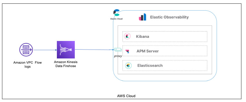
In the past, users would have to use an AWS Lambda function to transform the incoming data from VPC flow logs into an Amazon Simple Storage Service (Amazon S3) bucket before loading it into Kinesis Data Firehose or create a CloudWatch Logs subscription that sends any incoming log events that match defined filters to the Firehose delivery stream.
With this new integration, you can set up this configuration directly from your VPC flow logs to Kinesis Data Firehose and into Elastic Cloud. (Note that Elastic Cloud must be deployed on AWS.)
Let’s walk through the details of configuring Kinesis Data Firehose and Elastic, and demonstrate ingesting data.
Prerequisites
To set up this demonstration, make sure you have the following prerequisites:
- An account on Elastic Cloud and a deployed stack on AWS. Deploying this on AWS is required for Kinesis Data Firehose log ingestion. For instructions, refer to Installing the Elastic Stack.
- An AWS account with permissions to pull the necessary data from AWS.
- VPC flow logs enabled for the VPC where the application is deployed and configured to send data to Kinesis Data Firehose.
- A three-tier web architecture in AWS, which can ingest metrics from several AWS services.
We walk through installing general AWS integration components into the Elastic Cloud deployment to ensure Kinesis Data Firehose connectivity. Refer to the full list of services supported by the Elastic/AWS integration for more information.
Deploy Elastic on AWS
Follow the instructions on the Elastic registration page to get started on Elastic Cloud.
Once logged in to Elastic Cloud, create a deployment on AWS. It’s important to ensure that the deployment is on AWS. The Firehose delivery stream connects specifically to an endpoint that needs to be on AWS.
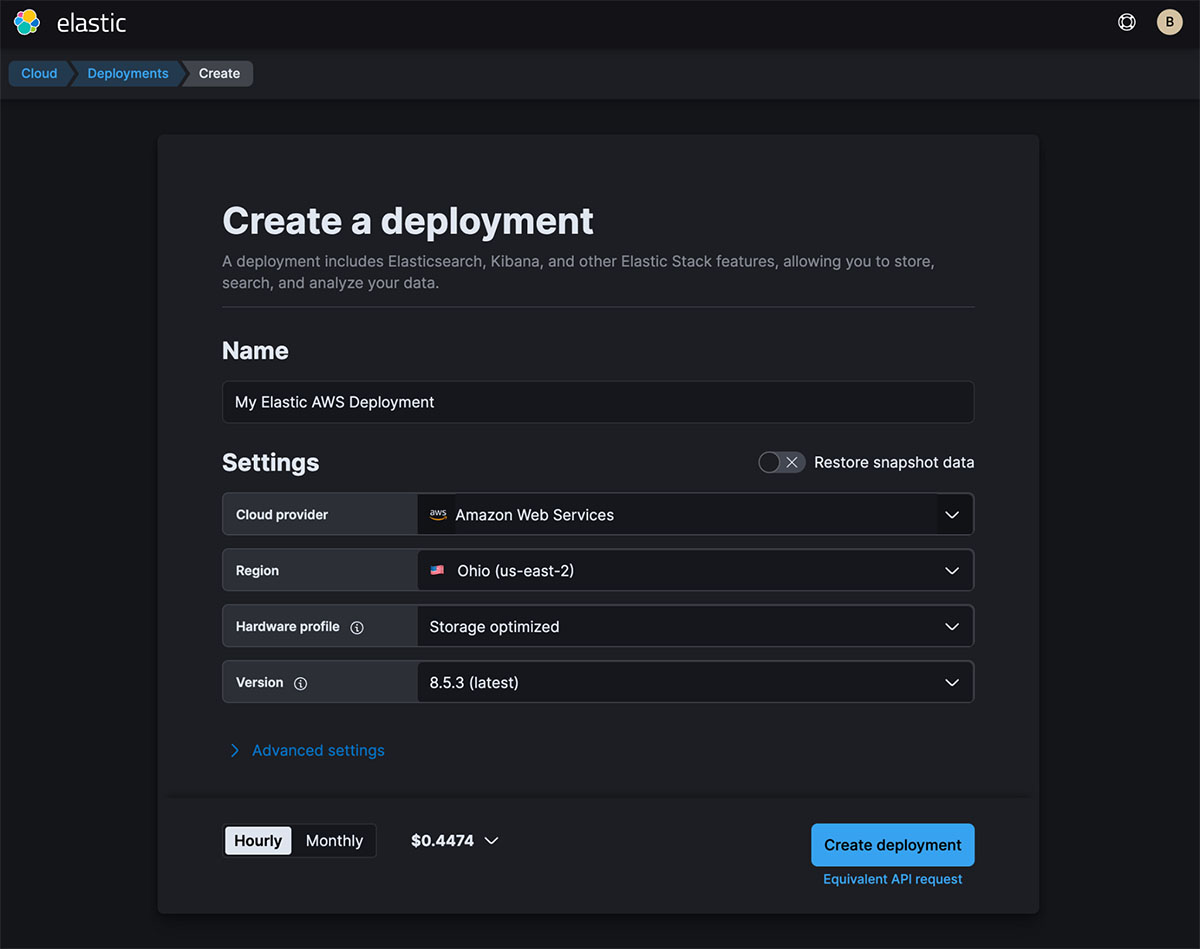
After you create your deployment, copy the Elasticsearch endpoint to use in a later step.

The endpoint should be an AWS endpoint, such as https://thevaa-cluster-01.es.us-east-1.aws.found.io.
Enable Elastic’s AWS integration
In your deployment’s Elastic Integration section, navigate to the AWS integration and choose Install AWS assets.
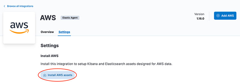
Configure a Firehose delivery stream
Create a new delivery stream on the Kinesis Data Firehose console. This is where you provide the endpoint you saved earlier. Refer to the following screenshot for the destination settings, and for more details, refer to Choose Elastic for Your Destination.

In this example, we are pulling in VPC flow logs via the data stream parameter we added (logs-aws.vpcflow-default). The parameter es\_datastream\_name can be configured with one of the following types of logs:
- logs-aws.cloudfront\_logs-default – AWS CloudFront logs
- logs-aws.ec2\_logs-default – Amazon Elastic Compute Cloud (Amazon EC2) logs in CloudWatch
- logs-aws.elb\_logs-default – Elastic Load Balancing logs
- logs-aws.firewall\_logs-default – AWS Network Firewall logs
- logs-aws.route53\_public\_logs-default – Amazon Route 53 public DNS queries logs
- logs-aws.route53\_resolver\_logs-default – Route 53 DNS queries and responses logs
- logs-aws.s3access-default – Amazon S3 server access log
- logs-aws.vpcflow-default – VPC flow logs
- logs-aws.waf-default – AWS WAF logs
Deploy your application
Follow the instructions on the GitHub repo and instructions in the AWS Three Tier Web Architecture workshop to deploy your application.
After you install the app, get your credentials from AWS to use with Elastic’s AWS integration.
There are several options for credentials:
- Use access keys directly
- Use temporary security credentials
- Use a shared credentials file
- Use an AWS Identity and Access Management (IAM) role Amazon Resource Name (ARN)
For more details, refer to AWS Credentials and AWS Permissions.
Configure VPC flow logs to send to Kinesis Data Firehose
In the VPC for the application you deployed, you need to configure your VPC flow logs and point them to the Firehose delivery stream.
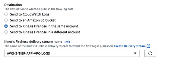
Validate the VPC flow logs
In the Elastic Observability view of the log streams, you should see the VPC flow logs coming in after a few minutes, as shown in the following screenshot.
Analyze VPC flow logs in Elastic
Now that you have VPC flow logs in Elastic Cloud, how can you analyze them? There are several analyses you can perform on the VPC flow log data:
- Use Elastic’s Analytics Discover capabilities to manually analyze the data
- Use Elastic Observability’s anomaly feature to identify anomalies in the logs
- Use an out-of-the-box dashboard to further analyze the data
Use Elastic’s Analytics Discover to manually analyze data
In Elastic Analytics, you can search and filter your data, get information about the structure of the fields, and display your findings in a visualization. You can also customize and save your searches and place them on a dashboard.
For a complete understanding of Discover and all of Elastic’s Analytics capabilities, refer to Discover.
For VPC flow logs, it’s important to understand the following:
- How many logs were accepted or rejected
- Where potential security violations occur (source IPs from outside the VPC)
- What port is generally being queried
For our example, we filter the logs on the following:
- Delivery stream name –
AWS-3-TIER-APP-VPC-LOGS - VPC flow log action –
REJECT - Time frame – 5 hours
- VPC network interface – Webserver 1 and Webserver 2 interfaces
We want to see what IP addresses are trying to hit our web servers. From that, we want to understand which IP addresses we’re getting the most REJECT actions from. We simply find the source.ip field and can quickly get a breakdown that shows 185.156.73.54 is the most rejected for the last 3 or more hours we’ve turned on VPC flow logs.
Additionally, we can create a visualization by choosing Visualize. We get the following donut chart, which we can add to a dashboard.

Additionally to IP addresses, we want to also see what port is being hit on our web servers.
We select the destination port field, and the pop-up shows us that port 8081 is being targeted. This port is generally used for the administration of Apache Tomcat. This is a potential security issue, however port 8081 is turned off for outside traffic, hence the REJECT.
Detect anomalies in Elastic Observability logs
In addition to Discover, Elastic Observability provides the ability to detect anomalies on logs using machine learning (ML). The feature has the following options:
- Log rate – Automatically detects anomalous log entry rates
- Categorization – Automatically categorizes log messages
For our VPC flow log, we enabled both features. When we look at what was detected for anomalous log entry rates, we get the following results.

Elastic immediately detected a spike in logs when we turned on VPC flow logs for our application. The rate change is being detected because we’re also ingesting VPC flow logs from another application for a couple of days prior to adding the application in this post.
We can drill down into this anomaly with ML and analyze further.
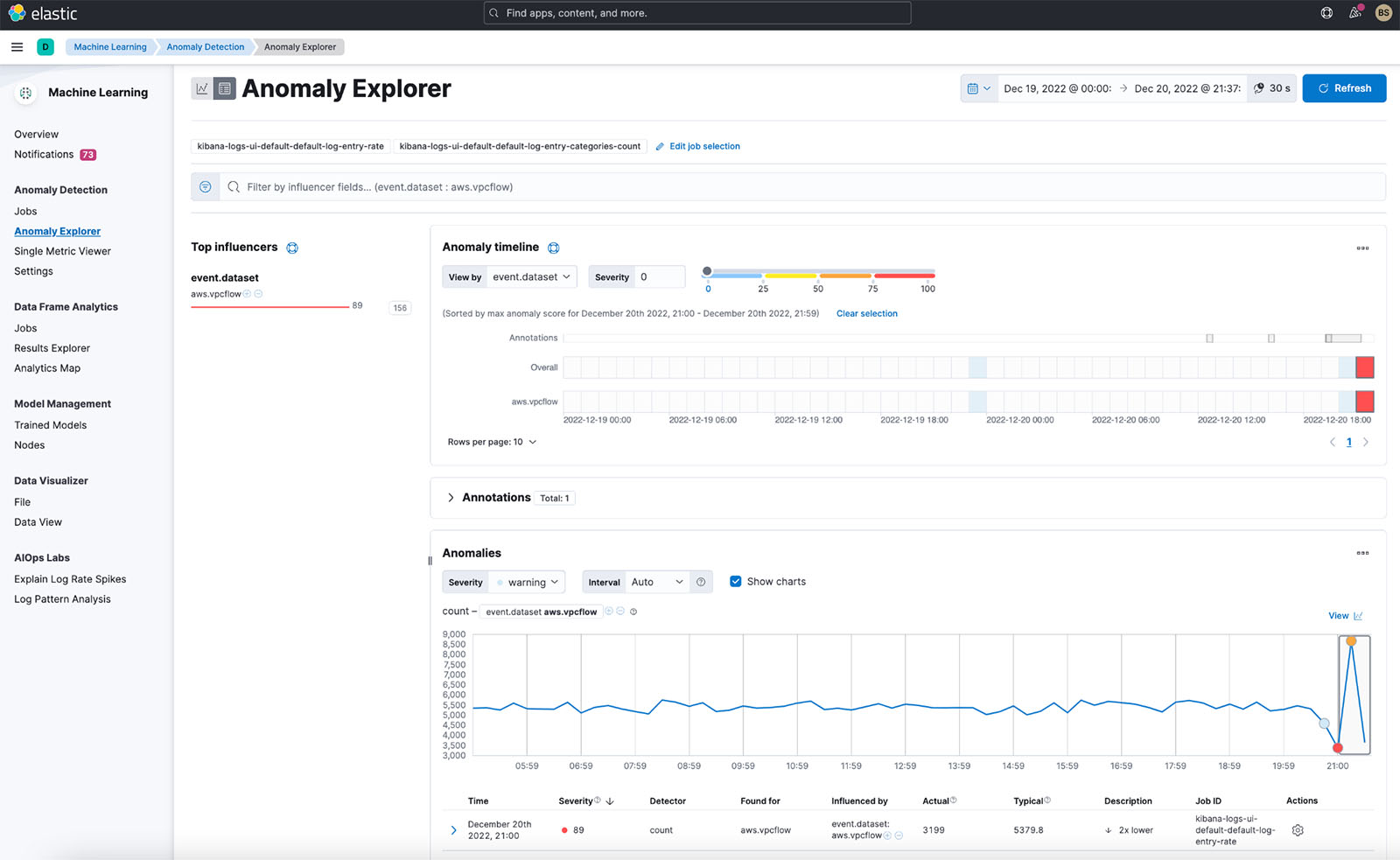
To learn more about the ML analysis you can utilize with your logs, refer to Machine learning.
Because we know that a spike exists, we can also use the Elastic AIOps Labs Explain Log Rate Spikes capability. Additionally, we’ve grouped them to see what is causing some of the spikes.

In the preceding screenshot, we can observe that a specific network interface is sending more VPC log flows than others. We can drill down into this further in Discover.
Use the VPC flow log dashboard
Finally, Elastic also provides an out-of-the-box dashboard to show the top IP addresses hitting your VPC, geographically where they are coming from, the time series of the flows, and a summary of VPC flow log rejects within the time frame.
You can enhance this baseline dashboard with the visualizations you find in Discover, as we discussed earlier.

Conclusion
This post demonstrated how to configure an integration with Kinesis Data Firehose and Elastic for efficient infrastructure monitoring of VPC flow logs in Elastic Kibana dashboards. Elastic offers flexible deployment options on AWS, supporting software as a service (SaaS), AWS Marketplace, and bring your own license (BYOL) deployments. Elastic also provides AWS Marketplace private offers. You have the option to deploy and run the Elastic Stack yourself within your AWS account, either free or with a paid subscription from Elastic. To get started, visit the Kinesis Data Firehose console and specify Elastic as the destination. To learn more, explore the Amazon Kinesis Data Firehose Developer Guide.
About the Authors
 Udayasimha Theepireddy is an Elastic Principal Solution Architect, where he works with customers to solve real world technology problems using Elastic and AWS services. He has a strong background in technology, business, and analytics.
 Antony Prasad Thevaraj is a Sr. Partner Solutions Architect in Data and Analytics at AWS. He has over 12 years of experience as a Big Data Engineer, and has worked on building complex ETL and ELT pipelines for various business units.
 Mostafa Mansour is a Principal Product Manager – Tech at Amazon Web Services where he works on Amazon Kinesis Data Firehose. He specializes in developing intuitive product experiences that solve complex challenges for customers at scale. When he’s not hard at work on Amazon Kinesis Data Firehose, you’ll likely find Mostafa on the squash court, where he loves to take on challengers and perfect his dropshots.
Amazon OpenSearch Service is a managed service that makes it simple to secure, deploy, and operate OpenSearch clusters at scale in the AWS Cloud. AWS IAM Identity Center (successor to AWS Single Sign-On) helps you securely create or connect your workforce identities and manage their access centrally across AWS accounts and applications. To build a strong least-privilege security posture, customers also wanted fine-grained access control to manage dashboard permission by user role. In this post, we demonstrate a step-by-step procedure to implement IAM Identity Center to OpenSearch Service via native SAML integration, and configure role-based access control in OpenSearch Dashboards by using group attributes in IAM Identity Center. You can follow the steps in this post to achieve both authentication and authorization for OpenSearch Service based on the groups configured in IAM Identity Center.
Solution overview
Let’s review how to map users and groups in IAM Identity Center to OpenSearch Service security roles. Backend roles in OpenSearch Service are used to map external identities or attributes of workgroups to pre-defined OpenSearch Service security roles.
The following diagram shows the solution architecture. Create two groups, assign a user to each group and edit attribute mappings in IAM Identity Center. If you have integrated IAM Identity Center with your Identity Provider (IdP), you can use existing users and groups mapped to your IdP for this test. The solution uses two roles: all\_access for administrators, and alerting\_full\_access for developers who are only allowed to manage OpenSearch Service alerts. You can set up backend role mapping in OpenSearch Dashboards by group ID. Based on the following diagram, you can map the role all\_access to the group Admin, and alerting\_full\_access to Developer. User janedoe is in the group Admin, and user johnstiles is in the group Developer.
Then you will log in as each user to verify the access control by looking at the different dashboard views.

Let’s get started!
Prerequisites
Complete the following prerequisite steps:
- Have an AWS account.
- Have an Amazon OpenSearch Service domain.
- Enable IAM Identity Center in the same Region as the OpenSearch Service domain.
- Test your users in IAM Identity Center (to create users, refer to Add users).
Enable SAML in Amazon OpenSearch Service and copy SAML parameters
To configure SAML in OpenSearch Service, complete the following steps:
- On the OpenSearch Service console, choose Domains in the navigation pane.
- Choose your domain.
- On the Security configuration tab, confirm that Fine-grained access control is enabled.

- On the Actions menu, choose Edit security configuration.

- Select Enable SAML authentication.
You can also configure SAML during domain creation if you are creating a new OpenSearch domain. For more information, refer to SAML authentication for OpenSearch Dashboards.
- Copy the values for Service provider entity ID and IdP-Initiated SSO URL.

Create a SAML application in IAM Identity Center
To create a SAML application in IAM Identity Center, complete the following steps:
- On the IAM Identity Center console, choose Applications in the navigation pane.
- Choose Add application.

- Select Add customer SAML 2.0 application, then choose Next.

- Enter your application name for Display name.
- Under IAM Identity Center metadata, choose Download to download the SAML metadata file.

- Under Application metadata, select Manually type your metadata values.
- For Application ACS URL, enter the IdP-initiated URL you copied earlier.
- For Application SAML audience, enter the service provider entity ID you copied earlier.
- Choose Submit.

- On the Actions menu, choose Edit attribute mappings.

- Create attributes and map the following values:
- Subject map to
${user:email}, the format is emailAddress. - Role map to
${user:groups}, the format is unspecified.
- Subject map to
- Choose Save changes.

- On the IAM Identity Center console, choose Groups in the navigation pane.
- Create two groups: Developer and Admin.

- Assign user
janedoeto the group Admin.

- Assign user johnstiles to the group Developer.

- Open the Admin group and copy the group ID.

Finish SAML configuration and map the SAML primary backend role
To complete your SAML configuration and map the SAML primary backend role, complete the following steps:
- On the OpenSearch Service console, choose Domains in the navigation pane.
- Open your domain and choose Edit security configuration.
- Under SAML authentication for OpenSearch Dashboards/Kibana, for Import IdP metadata, choose Import from XML file.
- Upload the IdP metadata downloaded from the IAM Identity Center metadata file.
The IdP entity ID will be auto populated.

- Under SAML master backend role, enter the group ID of the Admin group you copied earlier.
- For Roles key, enter Role for the SAML assertion.
This is because we defined and mapped Role to ${user:groups} as a SAML attribute in IAM Identity Center.
- Choose Save changes.

Configure backend role mapping for the Developer group
You have completely integrated IAM Identity Center with OpenSearch Service and mapped the Admin group as the primary role (all\_access) in OpenSearch Service. Now you will log in to OpenSearch Dashboards as Admin and configure mapping for the Developer group.
There are two ways to log in to OpenSearch Dashboards:
- OpenSearch Dashboards URL – On the OpenSearch Service console, navigate to your domain and choose the Dashboards URL under General Information. (For example,
https://opensearch-domain-name-random-keys.us-west-2.es.amazonaws.com/\_dashboards) - AWS access portal URL – On the IAM Identity Center console, choose Dashboard in the navigation pane and choose the access portal URL under Settings summary. (For example,
https://d-1234567abc.awsapps.com/start)
Complete the following steps:
- Log in as the user in the Admin group (
janedoe).

- Choose the tile for your OpenSearch Service application to be redirected to OpenSearch Dashboards.

- Choose the menu icon, then choose Security, Roles.

- Choose the
alerting\_full\_accessrole and on the Mapped users tab, choose Manage mapping.

- For Backend roles, enter the group ID of Developer.
- Choose Map to apply the change.

Now you have successfully mapped the Developer group to the alerting\_full\_access role in OpenSearch Service.

Verify permissions
To verify permissions, complete the following steps:
- Log out of the Admin account in OpenSearch Service as log in as a Developer user.
- Choose the OpenSearch Service application tile to be redirected to OpenSearch Dashboards.
You can see there are only alerting related features available on the drop-down menu. This Developer user can’t see all of the Admin features, such as Security.

Clean up
After you test the solution, remember to delete all of the resources you created to avoid incurring future charges:
- Delete your Amazon OpenSearch Service domain.
- Delete the SAML application, users, and groups in IAM Identity Center.
Conclusion
In the post, we walked through a solution of how to map roles in Amazon OpenSearch Service to groups in IAM Identity Center by using SAML attributes to achieve role-based access control for accessing OpenSearch Dashboards. We connected IAM Identity Center users to OpenSearch Dashboards, and also mapped predefined OpenSearch Service security roles to IAM Identity Center groups based on group attributes. This makes it easier to manage permissions without updating the mapping when new users belonging to the same workgroup want to log in to OpenSearch Dashboards. You can follow the same procedure to provide fine-grained access to workgroups based on team functions or compliance requirements.
About the Authors
 Scott Chang is a Solution Architecture at AWS based in San Francisco. He has over 14 years of hands-on experience in Networking also familiar with Security and Site Reliability Engineering. He works with one of major strategic customers in west region to design highly scalable, innovative and secure cloud solutions.
Muthu Pitchaimani is a Search Specialist with Amazon OpenSearch service. He builds large scale search applications and solutions. Muthu is interested in the topics of networking and security and is based out of Austin, Texas
Recently, one of the largest wireless carriers in North America revealed that hackers compromised a database of its customer information through unauthorized use of an API and acquired the personal details of millions of individuals, including names, addresses, phone numbers, and account numbers. Once identified, the company halted the malicious activity. However, investigations indicated that the data breach likely occurred months prior to being detected.
With the ever-increasing volume of data that organizations store in the cloud, malicious threats to their business sensitive data and resources will continue to grow alongside their online activity. Adversaries, also known as attackers, continue to use a variety of techniques to breach an organization’s security and compromise their systems, which can cause significant financial losses or damage to reputation or have legal consequences for the affected organization. To mitigate the damage caused, it is critically important for organizations to protect themselves by implementing various security measures and deploying tools to detect and respond to security threats. By being proactive, organizations can significantly reduce the risk of being victimized by cyber adversaries.
Amazon OpenSearch Service is a fully managed and scalable log analytics framework that you can use to ingest, store, and visualize data. You can use OpenSearch Service for a diverse set of data workloads including healthcare data, financial transactions information, application performance data, observability data, and much more. This managed service is valued for its ingest performance, scalability, low query latency, and its ability to analyze large datasets.
Security analytics with OpenSearch Service
Today, OpenSearch Service announces OpenSearch-powered security analytics, which includes features to monitor, analyze, and respond to potential security threats to your critical infrastructure. In this post, we discuss these new features and how to identify and remediate security threats.
Security analytics provide real-time visibility into potential threats across your infrastructure, enabling you to respond to security incidents quickly, thereby reducing the impact of any security breaches. It can also help you meet regulatory compliance requirements and improve your overall security posture.
Security analytics with OpenSearch is designed to gain visibility into a company’s infrastructure, monitor for anomalous activity, help detect potential security threats in real time, and trigger alerts to pre-configured destinations. You can monitor for malicious activity from your security event logs by continuously evaluating out-of-the-box security rules, and review auto generated security findings to aid your investigation. In addition, security analytics can generate automated alerts and send to a preconfigured destination of your choice such as Slack or email.
Security analytics is powered by the open-source OpenSearch project and deployed on OpenSearch Service with OpenSearch version 2.5 or higher. It includes the following key features:
- Out-of-the-box support for over 2,200 open-source Sigma security rules
- Support for log sources such as Windows, NetFlow, AWS CloudTrail, DNS, AD/LDAP, and more
- Detectors that auto generate findings based on the Sigma rules
- Automated alerts sent to preconfigured destinations
- A rules editor to create new custom rules or modify existing rules
- Visualizations to summarize findings and alerts trends
Sigma rules
Sigma is a generic signature format, expressed using YAML (yet another markup language), to describe significant events that occur in your logs in a simple and straightforward way. The format is portable across different SIEM implementations and fosters a community of threat hunters, so that you don’t have to reinvent the wheel if you change your SIEM implementation.
An example of a simple rule to detect the run of C:\Windows\System32\rundll32.exe, one of the most commonly used methods for launching malicious code on a Windows platform, could be the following YAML configuration:
After you import this rule into the security analytics rules repository and enable it with your detector, it auto generates a security finding when the preceding condition matches an incoming event log.
Security analytics components and concepts
The security analytics offering includes a number of tools and features elemental to its operation. The major components that comprise the plugin are summarized in the following sections.

Log types
OpenSearch supports several types of logs and provides out-of-the-box mappings for each. The log type is specified during the creation of a detector and includes the ability to customize field mappings for that detector. For a log type selected in a detector, security analytics automatically enables a relevant set of rules that run at the configured interval.
Detectors
Detectors are core components that you configure to identify a range of cybersecurity threats for a log type, across your data indexes. Detectors use custom rules and pre-packaged Sigma rules to evaluate events occurring in the system, automatically generating security findings from these events.
Rules
Rules, or threat detection rules, define the conditions applied to ingested log data to identify a security event. Security analytics provides prepackaged, open-source Sigma rules to detect common threats from your logs. Security analytics also supports importing, creating, and customizing rules to meet your requirements. Many rules are also mapped to an ever-growing knowledge base of adversary tactics and techniques maintained by the MITRE ATT&CK organization. You can take advantage of these options using either OpenSearch Dashboards or the APIs.
Findings
Findings are generated every time a detector matches a rule with a log event. Findings don’t necessarily point to imminent threats within the system, but they isolate an event of interest. Because they represent the result of a specific matched condition in a detector rule, findings include a unique combination of select rules, a log type, and a rule severity.
Alerts
When defining a detector, you can specify one or more conditions that trigger an alert. When an event triggers an alert, the system sends a notification to a preferred channel, such as Slack or email. The alert can be triggered when the detector matches one or multiple rules. You can also create a notification message with a customized subject line and message body.
Taking the tool for a test drive
With an understanding of these fundamental concepts, let’s navigate to the security analytics interface in OpenSearch Dashboards. Security analytics also provides a robust set of configuration APIs.
Overview page
After you have logged in to OpenSearch Dashboards and navigate to the security analytics overview page, you’re presented with the current state of the detectors you are monitoring. You can see a summary view comprised of multiple visualizations. The following chart, for example, shows the findings and alerts trend for various log types over a given period of time.

As you scroll down on the summary page, you can review your most recent findings and alerts.

Additionally, you can see a distribution of the most frequently triggered rules across all the active detectors. This can help you detect and investigate different types of malicious activities across log types.

Finally, you can view the status of configured detectors. From this panel, you can also navigate to the create detector workflow.

Creating a detector
In the previous section, we reviewed the overview page. Now, let’s walkthrough the create detector workflow. One of the best things about security analytics are the prepackaged rules. You don’t have to write your own. You can use the prepackaged rules to get up and running quickly! In the following example, we show you how to create a detector with prepackaged rules for your Windows logs.
- In the Dashboards navigation pane, under Security Analytics, choose Detectors.
- Choose Create Detector to create a new detector.
- First, give it a name and a data source to query. The data source can be a pattern or specific index.

- When you select a Log type, all matching rules are automatically loaded and enabled by default. In this example, we select Windows logs to help narrow the set of rules applied to this detector. As an optional step, you can choose to selectively enable or disable one or more rules. See an example rules selection panel below.

- Specify a schedule to run the rules and select Next.

- Configure any necessary field mappings per your rule.
You have two field mapping sections to optionally review. Default mapped fields provide pre-configured field mappings for the specific log type and enabled rules; you can skip this section unless you need to change the mappings. Additional mappings can be configured in the Pending field mappings section.
- First, give it a name and a data source to query. The data source can be a pattern or specific index.
- Configure the alerts.
The final step of setting up a detector is to configure the alerts and review your configuration. Note that each detector can generate multiple findings or alerts, and you have the option to customize the alert destination based on a rule match criterion such as severity, tags etc. In this example, we show you how to match a single rule that monitors a password dump to a host file system (QuarksPwDumps Dump File) and send the alert to a destination of your choice.- First, define the name of the alert.
- Set up the criticality based on configurations in the rule and select the tags.

- Give the alert a severity and select a channel.
If you need to create a new channel, there is a breadcrumb that sends you to the Notifications feature. You can create additional channels needed.
- Review the configuration and Create the detector. Once the detector is active, any time a rule is matched for your incoming logs, it will automatically generate a security finding and alert (if configured).

Configuring custom rules
One of the key capabilities of security analytics is defining custom rules and being able to import rules created by others such as a community of threat hunters. As mentioned before, security analytics includes over 2200 rules out of the box. In some cases, you may want to create your own rules. If you navigate to the Rules page, you have the option to create your own rule.

The rules editor allows you to provide a custom rule that it will automatically validate. Once created, the rule is included in the rules library, helping you to customize your threat hunting needs.

Conclusion
Many organizations struggle with the high cost of commercial alternatives and are required to duplicate their data across multiple systems that generate specific insights. OpenSearch Service security analytics provides an open-source alternative to businesses that seek to reduce the cost of their security products. There is no additional charge for security analytics, and you can customize it to meet the security requirements of your organization. With simple workflows and prepackaged security content, security analytics enables your security teams to detect potential threats quickly while providing the tools to help with security investigations.
To get started, create or upgrade your existing Amazon OpenSearch Service domain to OpenSearch version 2.5. To learn more about security analytics, see documentation.
About the Authors
 Kevin Fallis (@AWSCodeWarrior) is an Principal AWS Specialist Search Solutions Architect. His passion at AWS is to help customers leverage the correct mix of AWS services to achieve success for their business goals. His after-work activities include family, DIY projects, carpentry, playing drums, and all things music.
 Jimish Shah is a Senior Product Manager at AWS with 15+ years of experience bringing products to market in log analytics, cybersecurity, and IP video streaming. He’s passionate about launching products that offer delightful customer experiences, and solve complex customer problems. In his free time, he enjoys exploring cafes, hiking, and taking long walks
Amazon Managed Streaming for Apache Kafka (Amazon MSK) is an AWS streaming data service that manages Apache Kafka infrastructure and operations, making it easy for developers and DevOps managers to run Apache Kafka applications and Kafka Connect connectors on AWS, without the need to become experts in operating Apache Kafka. Amazon MSK operates, maintains, and scales Apache Kafka clusters, provides enterprise-grade security features out of the box, and has built-in AWS integrations that accelerate development of streaming data applications. You can easily get started by creating an MSK cluster using the AWS Management Console with a few clicks.
When creating a cluster, you must choose a cluster type from two options: provisioned or serverless. Choosing the best cluster type for each workload depends on the type of workload and your DevOps preferences. Amazon MSK provisioned clusters offer more flexibility in how you scale, configure, and optimize your cluster. Amazon MSK Serverless, on the other hand, makes scaling, load management, and operation of the cluster easier for you. With MSK Serverless, you can run your applications without having to configure, manage the infrastructure, or optimize clusters, and you pay for the data volume you stream and retain. MSK Serverless fully manages partitions, including monitoring as well as ensuring an even balance of partition distribution across brokers in the cluster (auto-balancing).
In this post, I examine a use case with the fictitious company AnyCompany, who plans to use Amazon MSK for two applications. They must decide between provisioned or serverless cluster types. I describe a process by which they work backward from the applications’ requirements to find the best MSK cluster type for their workloads, including how the organizational structure and application requirements are relevant in finding the best offering. Lastly, I examine the requirements and their relationship to Amazon MSK features.
Use case
AnyCompany is an enterprise organization that is ready to move two of their Kafka applications to Amazon MSK.
The first is a large ecommerce platform, which is a legacy application that currently uses a self-managed Apache Kafka cluster run in their data centers. AnyCompany wants to migrate this application to the AWS Cloud and use Amazon MSK to reduce maintenance and operations overhead. AnyCompany has a DataOps team that has been operating self-managed Kafka clusters in their data centers for years. AnyCompany wants to continue using the DataOps team to manage the MSK cluster on behalf of the development team. There is very little flexibility for code changes. For example, a few modules of the application require plaintext communication and access to the Apache ZooKeeper cluster that comes with an MSK cluster. The ingress throughput for this application doesn’t fluctuate often. The ecommerce platform only experiences a surge in user activity during special sales events. The DataOps team has a good understanding of this application’s traffic pattern, and are confident that they can optimize an MSK cluster by setting some custom broker-level configurations.
The second application is a new cloud-native gaming application currently in development. AnyCompany hopes to launch this gaming application soon followed by a marketing campaign. Throughput needs for this application are unknown. The application is expected to receive high traffic initially, then user activity should decline gradually. Because the application is going to launch first in the US, traffic during the day is expected to be higher than at night. This application offers a lot of flexibility in terms of Kafka client version, encryption in transit, and authentication. Because this is a cloud-native application, AnyCompany hopes they can delegate full ownership of its infrastructure to the development team.
Solution overview
Let’s examine a process that helps AnyCompany decide between the two Amazon MSK offerings. The following diagram shows this process at a high level.
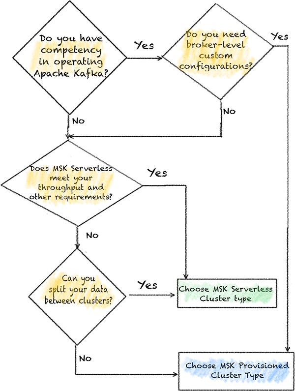
In the following sections, I explain each step in detail and the relevant information that AnyCompany needs to collect before they make a decision.
Competency in Apache Kafka
AWS recommends a list of best practices to follow when using the Amazon MSK provisioned offering. Amazon MSK provisioned, offers more flexibility so you make scaling decisions based on what’s best for your workloads. For example, you can save on cost by consolidating a group of workloads into a single cluster. You can decide which metrics are important to monitor and optimize your cluster through applying custom configurations to your brokers. You can choose your Apache Kafka version, among different supported versions, and decide when to upgrade to a new version. Amazon MSK takes care of applying your configuration and upgrading each broker in a rolling fashion.
With more flexibility, you have more responsibilities. You need to make sure your cluster is right-sized at any time. You can achieve this by monitoring a set of cluster-level, broker-level, and topic-level metrics to ensure you have enough resources that are needed for your throughput. You also need to make sure the number of partitions assigned to each broker doesn’t exceed the numbers suggested by Amazon MSK. If partitions are unbalanced, you need to even-load them across all brokers. If you have more partitions than recommended, you need to either upgrade brokers to a larger size or increase the number of brokers in your cluster. There are also best practices for the number of TCP connections when using AWS Identity and Access Management (IAM) authentication.
An MSK Serverless cluster takes away the complexity of right-sizing clusters and balancing partitions across brokers. This makes it easy for developers to focus on writing application code.
AnyCompany has an experienced DataOps team who are familiar with scaling operations and best practices for the MSK provisioned cluster type. AnyCompany can use their DataOps team’s Kafka expertise for building automations and easy-to-follow standard procedures on behalf of the ecommerce application team. The gaming development team is an exception, because they are expected to take the full ownership of the infrastructure.
In the following sections, I discuss other steps in the process before deciding which cluster type is right for each application.
Custom configuration
In certain use cases, you need to configure your MSK cluster differently from its default settings. This could be due to your application requirements. For example, AnyCompany’s ecommerce platform requires setting up brokers such that the default retention period for all topics is set to 72 hours. Also, topics should be or auto-created when they are requested and don’t exist.
The Amazon MSK provisioned offering provides a default configuration for brokers, topics, and Apache ZooKeeper nodes. It also allows you to create custom configurations and use them to create new MSK clusters or update existing clusters. An MSK cluster configuration consists of a set of properties and their corresponding values.
MSK Serverless doesn’t allow applying broker-level configuration. This is because AWS takes care of configuring and managing the backend nodes. It takes away the heavy lifting of configuring the broker nodes. You only need to manage your applications’ topics. To learn more, refer to the list of topic-level configurations that MSK Serverless allows you to change.
Unlike the ecommerce platform, AnyCompany’s gaming application doesn’t need broker-level custom configuration. The developers want to set the retention.ms and max.message.bytes per each topic only.
Application requirements
Apache Kafka applications differ in terms of their security; the way they connect, write, or read data; data retention period; and scaling patterns. For example, some applications can only scale vertically, whereas other applications can scale only horizontally. Although a flexible application can work with encryption in transit, a legacy application may only be able to communicate in plaintext format.
Cluster-level quotas
Amazon MSK enforces some quotas to ensure the performance, reliability, and availability of the service for all customers. These quotas are subject to change at any time. To access the latest values for each dimension, refer to Amazon MSK quota. Note that some of the quotas are soft limits and can be increased using a support ticket.
When choosing a cluster type in Amazon MSK, it’s important to understand your application requirements and compare those against quotas in relation with each offering. This makes sure you choose the best cluster type that meets your goals and application’s needs. Let’s examine how you can calculate the throughput you need and other important dimensions you need to compare with Amazon MSK quotas:
- Number of clusters per account – Amazon MSK may have quotas for how many clusters you can create in a single AWS account. If this is limiting your ability to create more clusters, you can consider creating those in multiple AWS accounts and using secure connectivity patterns to provide access to your applications.
- Message size – You need to make sure the maximum message size that your producer writes for a single message is lower than the configured size in the MSK cluster. MSK provisioned clusters allow you to change the default value in a custom configuration. If you choose MSK Serverless, check this value in Amazon MSK quota. The average message size is helpful when calculating the total ingress or egress throughput of the cluster, which I demonstrate later in this post.
- Message rate per second – This directly influences total ingress and egress throughput of the cluster. Total ingress throughput equals the message rate per second multiplied by message size. You need to make sure your producer is configured for optimal throughput by adjusting
batch.sizeandlinger.msproperties. If you’re choosing MSK Serverless, you need to make sure you configure your producer to optimal batches with the rate that is lower than its request rate quota. - Number of consumer groups – This directly influences the total egress throughput of the cluster. Total egress throughput equals the ingress throughput multiplied by the number of consumer groups. If you’re choosing MSK Serverless, you need to make sure your application can work with these quotas.
- Maximum number of partitions – Amazon MSK provisioned recommends not exceeding certain limits per broker (depending the broker size). If the number of partitions per broker exceeds the maximum value specified in the previous table, you can’t perform certain upgrade or update operations. MSK Serverless also has a quota of maximum number of partitions per cluster. You can request to increase the quota by creating a support case.
Partition-level quotas
Apache Kafka organizes data in structures called topics. Each topic consists of a single or many partitions. Partitions are the degree of parallelism in Apache Kafka. The data is distributed across brokers using data partitioning. Let’s examine a few important Amazon MSK requirements, and how you can make sure which cluster type works better for your application:
- Maximum throughput per partition – MSK Serverless automatically balances the partitions of your topic between the backend nodes. It instantly scales when your ingress throughput increases. However, each partition has a quota of how much data it accepts. This is to ensure the data is distributed evenly across all partitions and backend nodes. In an MSK Serverless cluster, you need to create your topic with enough partitions such that the aggregated throughput is equal to the maximum throughput your application requires. You also need to make sure your consumers read data with a rate that is below the maximum egress throughput per partition quota. If you’re using Amazon MSK provisioned, there is no partition-level quota for write and read operations. However, AWS recommends you monitor and detect hot partitions and control how partitions should balance among the broker nodes.
- Data storage – The amount of time each message is kept in a particular topic directly influences the total amount of storage needed for your cluster. Amazon MSK allows you to manage the retention period at the topic level. MSK provisioned clusters allow broker-level configuration to set the default data retention period. MSK Serverless clusters allow unlimited data retention, but there is a separate quota for the maximum data that can be stored in each partition.
Security
Amazon MSK recommends that you secure your data in the following ways. Availability of the security features varies depending on the cluster type. Before making a decision about your cluster type, check if your preferred security options are supported by your choice of cluster type.
- Encryption at rest – Amazon MSK integrates with AWS Key Management Service (AWS KMS) to offer transparent server-side encryption. Amazon MSK always encrypts your data at rest. When you create an MSK cluster, you can specify the KMS key that you want Amazon MSK to use to encrypt your data at rest.
- Encryption in transit – Amazon MSK uses TLS 1.2. By default, it encrypts data in transit between the brokers of your MSK cluster. You can override this default when you create the cluster. For communication between clients and brokers, you must specify one of the following settings:
- Only allow TLS encrypted data. This is the default setting.
- Allow both plaintext and TLS encrypted data.
- Only allow plaintext data.
- Authentication and authorization – Use IAM to authenticate clients and allow or deny Apache Kafka actions. Alternatively, you can use TLS or SASL/SCRAM to authenticate clients, and Apache Kafka ACLs to allow or deny actions.
Cost of ownership
Amazon MSK helps you avoid spending countless hours and significant resources just managing your Apache Kafka cluster, adding little or no value to your business. With a few clicks on the Amazon MSK console, you can create highly available Apache Kafka clusters with settings and configuration based on Apache Kafka’s deployment best practices. Amazon MSK automatically provisions and runs Apache Kafka clusters. Amazon MSK continuously monitors cluster health and automatically replaces unhealthy nodes with no application downtime. In addition, Amazon MSK secures Apache Kafka clusters by encrypting data at rest and in transit. These capabilities can significantly reduce your Total Cost of Ownership (TCO).
With MSK provisioned clusters, you can specify and then scale cluster capacity to meet your needs. With MSK Serverless clusters, you don’t need to specify or scale cluster capacity. MSK Serverless automatically scales the cluster capacity based on the throughput, and you only pay per GB of data that your producers write to and your consumers read from the topics in your cluster. Additionally, you pay an hourly rate for your serverless clusters and an hourly rate for each partition that you create. The MSK Serverless cluster type generally offers a lower cost of ownership by taking away the cost of engineering resources needed for monitoring, capacity planning, and scaling MSK clusters. However, if your organization has a DataOps team with Kafka competency, you can use this competency to operate optimized MSK provisioned clusters. This allows you to save on Amazon MSK costs by consolidating several Kafka applications into a single cluster. There are a few critical considerations to decide when and how to split your workloads between multiple MSK clusters.
Apache ZooKeeper
Apache ZooKeeper is a service included in Amazon MSK when you create a cluster. It manages the Apache Kafka metadata and acts as a quorum controller for leader elections. Although interacting with ZooKeeper is not a recommended pattern, some Kafka applications have a dependency to connect directly to ZooKeeper. During the migration to Amazon MSK, you may find a few of these applications in your organization. This could be because they use an older version of the Kafka client library or other reasons. For example, applications that help with Apache Kafka admin operations or visibility such as Cruise Control usually need this kind of access.
Before you choose your cluster type, you first need to check which offering provides direct access to the ZooKeeper cluster. As of writing this post, only Amazon MSK provisioned provides direct access to ZooKeeper.
How AnyCompany chooses their cluster types
AnyCompany first needs to collect some important requirements about each of their applications. The following table shows these requirements. The rows marked with an asterisk (*) are calculated based on the values in previous rows.
| Dimension | Ecommerce Platform | Gaming Application |
| Message rate per second | 150,000 | 1,000 |
| Maximum message size | 15 MB | 1 MB |
| Average message size | 30 KB | 15 KB |
| * Ingress throughput (average message size * message rate per second) | 4.5GBps | 15MBps |
| Number of consumer groups | 2 | 1 |
| * Outgress throughput (ingress throughput * number of consumer groups) | 9 GBps | 15 MBps |
| Number of topics | 100 | 10 |
| Average partition per topic | 100 | 5 |
| * Total number of partitions (number of topics * average partition per topic) | 10,000 | 50 |
| * Ingress per partition (ingress throughput / total number of partitions) | 450 KBps | 300 KBps |
| * Outgress per partition (outgress throughput / total number of partitions) | 900 KBps | 300 KBps |
| Data retention | 72 hours | 168 hours |
| * Total storage needed (ingress throughput * retention period in seconds) | 1,139.06 TB | 1.3 TB |
| Authentication | Plaintext and SASL/SCRAM | IAM |
| Need ZooKeeper access | Yes | No |
For the gaming application, AnyCompany doesn’t want to use their in-house Kafka competency to support an MSK provisioned cluster. Also, the gaming application doesn’t need custom configuration, and its throughput needs are below the quotas set by the MSK Serverless cluster type. In this scenario, an MSK Serverless cluster makes more sense.
For the e-commerce platform, AnyCompany wants to use their Kafka competency. Moreover, their throughput needs exceed the MSK Serverless quotas, and the application requires some broker-level custom configuration. The ecommerce platform also can’t split between multiple clusters. Because of these reasons, AnyCompany chooses the MSK provisioned cluster type in this scenario. Additionally, AnyCompany can save more on cost with the Amazon MSK provisioned pricing model. Their throughput is consistent at most times and AnyCompany wants to use their DataOps team to optimize a provisioned MSK cluster and make scaling decisions based on their own expertise.
Conclusion
Choosing the best cluster type for your applications may seem complicated at first. In this post, I showed a process that helps you work backward from your application’s requirement and the resources available to you. MSK provisioned clusters offer more flexibility in how you scale, configure, and optimize your cluster. MSK Serverless, on the other hand, is a cluster type that makes it easier for you to run Apache Kafka clusters without having to manage compute and storage capacity. I generally recommend you begin with MSK Serverless if your application doesn’t require broker-level custom configurations, and your application throughput needs don’t exceed the quotas for the MSK Serverless cluster type. Sometimes it’s best to split your workloads between multiple MSK Serverless clusters, but if that isn’t possible, you may need to consider an MSK provisioned cluster. To operate an optimized MSK provisioned cluster, you need to have Kafka competency within your organization.
For further reading on Amazon MSK, visit the official product page.
About the author
Ali Alemi is a Streaming Specialist Solutions Architect at AWS. Ali advises AWS customers with architectural best practices and helps them design real-time analytics data systems that are reliable, secure, efficient, and cost-effective. He works backward from customers’ use cases and designs data solutions to solve their business problems. Prior to joining AWS, Ali supported several public sector customers and AWS consulting partners in their application modernization journey and migration to the cloud.
Since the deluge of big data over a decade ago, many organizations have learned to build applications to process and analyze petabytes of data. Data lakes have served as a central repository to store structured and unstructured data at any scale and in various formats. However, as data processing at scale solutions grow, organizations need to build more and more features on top of their data lakes. One important feature is to run different workloads such as business intelligence (BI), Machine Learning (ML), Data Science and data exploration, and Change Data Capture (CDC) of transactional data, without having to maintain multiple copies of data. Additionally, the task of maintaining and managing files in the data lake can be tedious and sometimes complex.
Table formats like Apache Iceberg provide solutions to these issues. They enable transactions on top of data lakes and can simplify data storage, management, ingestion, and processing. These transactional data lakes combine features from both the data lake and the data warehouse. You can simplify your data strategy by running multiple workloads and applications on the same data in the same location. However, using these formats requires building, maintaining, and scaling infrastructure and integration connectors that can be time-consuming, challenging, and costly.
In this post, we show how you can build a serverless transactional data lake with Apache Iceberg on Amazon Simple Storage Service (Amazon S3) using Amazon EMR Serverless and Amazon Athena. We provide an example for data ingestion and querying using an ecommerce sales data lake.
Apache Iceberg overview
Iceberg is an open-source table format that brings the power of SQL tables to big data files. It enables ACID transactions on tables, allowing for concurrent data ingestion, updates, and queries, all while using familiar SQL. Iceberg employs internal metadata management that keeps track of data and empowers a set of rich features at scale. It allows you to time travel and roll back to old versions of committed data transactions, control the table’s schema evolution, easily compact data, and employ hidden partitioning for fast queries.
Iceberg manages files on behalf of the user and unlocks use cases such as:
- Concurrent data ingestion and querying, including streaming and CDC
- BI and reporting with expressive simple SQL
- Empowering ML feature stores and training sets
- Compliance and regulations workloads, such as GDPR find and forget
- Reinstating late-arriving data, which is dimensions data arriving later than the fact data. For example, the reason for a flight delay may arrive well after the fact that the fligh is delayed.
- Tracking data changes and rollback
Build your transactional data lake on AWS
You can build your modern data architecture with a scalable data lake that integrates seamlessly with an Amazon Redshift powered cloud warehouse. Moreover, many customers are looking for an architecture where they can combine the benefits of a data lake and a data warehouse in the same storage location. In the following figure, we show a comprehensive architecture that uses the modern data architecture strategy on AWS to build a fully featured transactional data lake. AWS provides flexibility and a wide breadth of features to ingest data, build AI and ML applications, and run analytics workloads without having to focus on the undifferentiated heavy lifting.
Data can be organized into three different zones, as shown in the following figure. The first zone is the raw zone, where data can be captured from the source as is. The transformed zone is an enterprise-wide zone to host cleaned and transformed data in order to serve multiple teams and use cases. Iceberg provides a table format on top of Amazon S3 in this zone to provide ACID transactions, but also to allow seamless file management and provide time travel and rollback capabilities. The business zone stores data specific to business cases and applications aggregated and computed from data in the transformed zone.
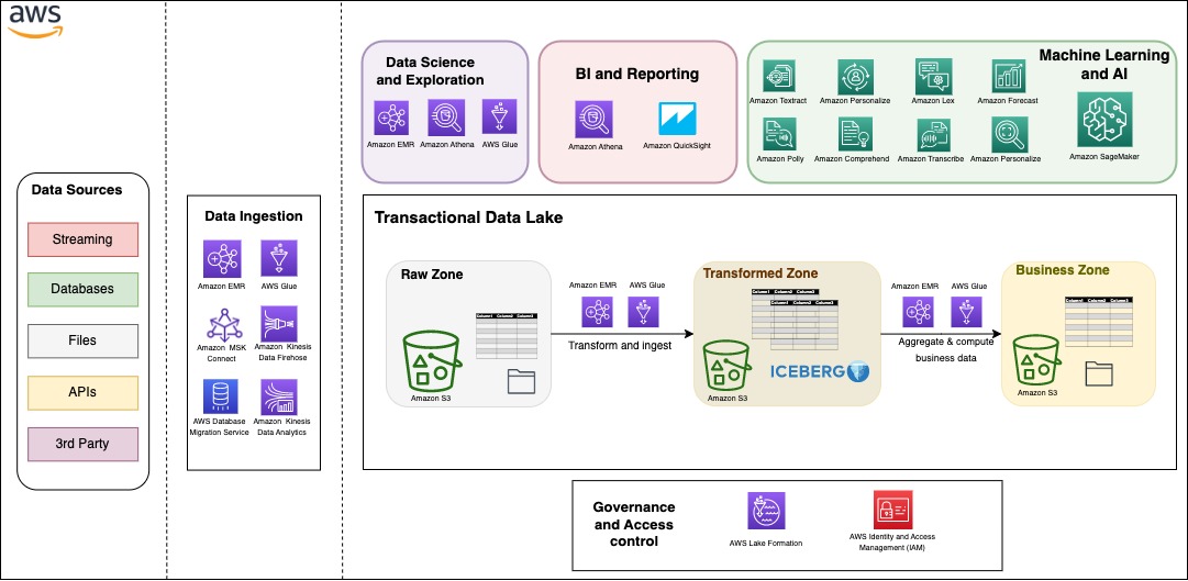
One important aspect to a successful data strategy for any organization is data governance. On AWS, you can implement a thorough governance strategy with fine-grained access control to the data lake with AWS Lake Formation.
Serverless architecture overview
In this section, we show you how to ingest and query data in your transactional data lake in a few steps. EMR Serverless is a serverless option that makes it easy for data analysts and engineers to run Spark-based analytics without configuring, managing, and scaling clusters or servers. You can run your Spark applications without having to plan capacity or provision infrastructure, while paying only for your usage. EMR Serverless supports Iceberg natively to create tables and query, merge, and insert data with Spark. In the following architecture diagram, Spark transformation jobs can load data from the raw zone or source, apply the cleaning and transformation logic, and ingest data in the transformed zone on Iceberg tables. Spark code can run instantaneously on an EMR Serverless application, which we demonstrate later in this post.
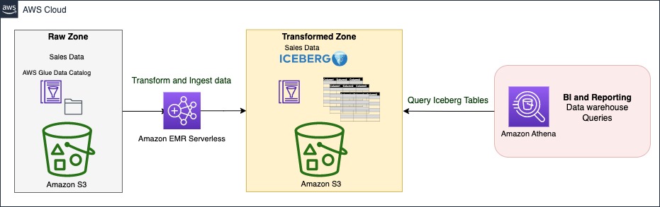
The Iceberg table is synced with the AWS Glue Data Catalog. The Data Catalog provides a central location to govern and keep track of the schema and metadata. With Iceberg, ingestion, update, and querying processes can benefit from atomicity, snapshot isolation, and managing concurrency to keep a consistent view of data.
Athena is a serverless, interactive analytics service built on open-source frameworks, supporting open-table and file formats. Athena provides a simplified, flexible way to analyze petabytes of data where it lives. To serve BI and reporting analysis, it allows you to build and run queries on Iceberg tables natively and integrates with a variety of BI tools.
Sales data model
Star schema and its variants are very popular for modeling data in data warehouses. They implement one or more fact tables and dimension tables. The fact table stores the main transactional data from the business logic with foreign keys to dimensional tables. Dimension tables hold additional complementary data to enrich the fact table.
In this post, we take the example of sales data from the TPC-DS benchmark. We zoom in on a subset of the schema with the web\_sales fact table, as shown in the following figure. It stores numeric values about sales cost, ship cost, tax, and net profit. Additionally, it has foreign keys to dimensional tables like date\_dim, time\_dim, customer, and item. These dimensional tables store records that give more details. For instance, you can show when a sale took place by which customer for which item.
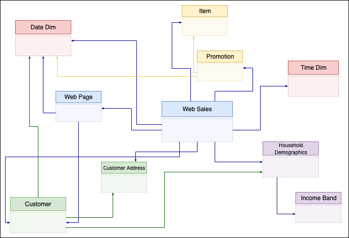
Dimension-based models have been used extensively to build data warehouses. In the following sections, we show how to implement such a model on top of Iceberg, providing data warehousing features on top of your data lake, and run different workloads in the same location. We provide a complete example of building a serverless architecture with data ingestion using EMR Serverless and Athena using TPC-DS queries.
Prerequisites
For this walkthrough, you should have the following prerequisites:
- An AWS account
- Basic knowledge about data management and SQL
Deploy solution resources with AWS CloudFormation
We provide an AWS CloudFormation template to deploy the data lake stack with the following resources:
- Two S3 buckets: one for scripts and query results, and one for the data lake storage
- An Athena workgroup
- An EMR Serverless application
- An AWS Glue database and tables on external public S3 buckets of TPC-DS data
- An AWS Glue database for the data lake
- An AWS Identity and Access Management (IAM) role and polices
Complete the following steps to create your resources:
- Launch the CloudFormation stack:

This automatically launches AWS CloudFormation in your AWS account with the CloudFormation template. It prompts you to sign in as needed.
- Keep the template settings as is.
- Check the I acknowledge that AWS CloudFormation might create IAM resources box.
- Choose Submit
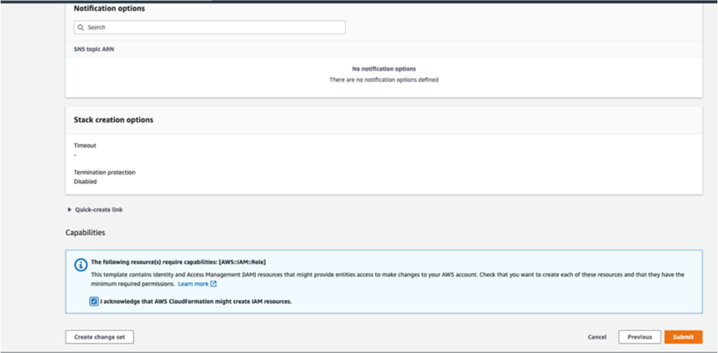
When the stack creation is complete, check the Outputs tab of the stack to verify the resources created.
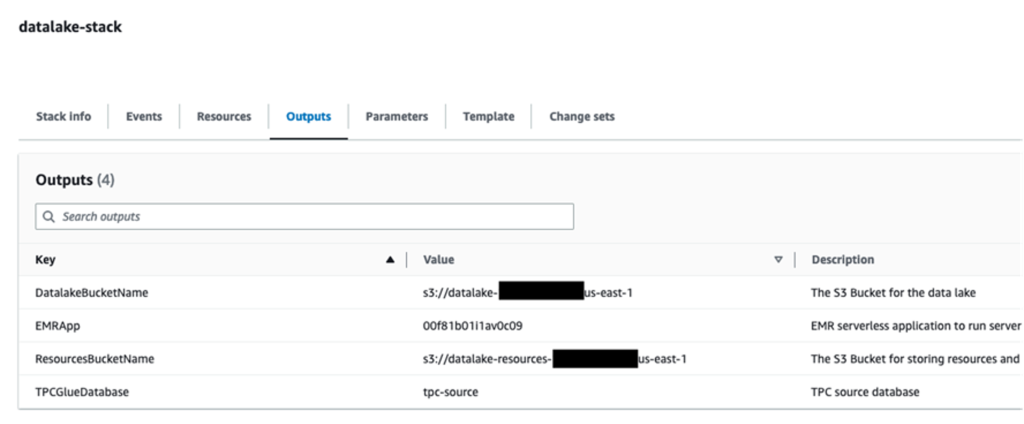
Upload Spark scripts to Amazon S3
Complete the following steps to upload your Spark scripts:
- Download the following scripts: ingest-iceberg.py and update-item.py.
- On the Amazon S3 console, go to the
datalake-resources-<AccountID>-us-east-1bucket you created earlier. - Create a new folder named
scripts. - Upload the two PySpark scripts:
ingest-iceberg.pyandupdate-item.py.
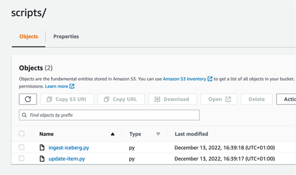
Create Iceberg tables and ingest TPC-DS data
To create your Iceberg tables and ingest the data, complete the following steps:
- On the Amazon EMR console, choose EMR Serverless in the navigation pane.
- Choose Manage applications.
- Choose the application
datalake-app.

- Choose Start application.
Once started, it will provision the pre-initialized capacity as configured at creation (one Spark driver and two Spark executors). The pre-initialized capacity are resources that will be provisioned when you start your application. They can be used instantly when you submit jobs. However, they incur charges even if they’re not used when the application is in a started state. By default, the application is set to stop when idle for 15 minutes.
Now that the EMR application has started, we can submit the Spark ingest job ingest-iceberg.py. The job creates the Iceberg tables and then loads data from the previously created AWS Glue Data Catalog tables on TPC-DS data in an external bucket.
- Navigate to the
datalake-app. - On the Job runs tab, choose Submit job.
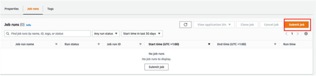
- For Name, enter
ingest-data. - For Runtime role, choose the IAM role created by the CloudFormation stack.
- For Script location, enter the S3 path for your resource bucket (
datalake-resource-<####>-us-east-1>scripts>ingest-iceberg.py).
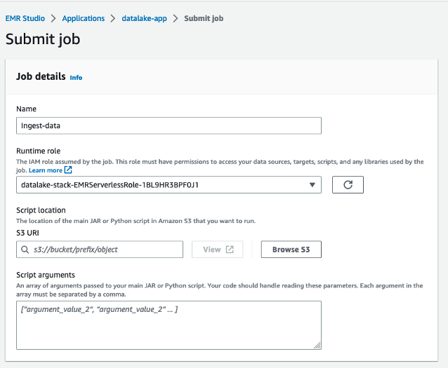
- Under Spark properties, choose Edit in text.
- Enter the following properties, replacing <BUCKET\_NAME> with your data lake bucket name
datalake-<####>-us-east-1(not datalake-resources)
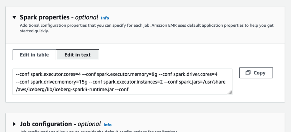
- Submit the job.
You can monitor the job progress. 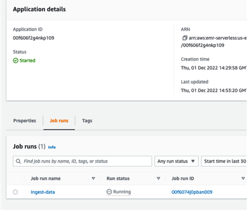
Query Iceberg tables
In this section, we provide examples of data warehouse queries from TPC-DS on the Iceberg tables.
- On the Athena console, open the query editor.
- For Workgroup, switch to
DatalakeWorkgroup.

- Choose Acknowledge.
 The queries in
 DatalakeWorkgroup will run on Athena engine version 3.
- On the Saved queries tab, choose a query to run on your Iceberg tables.
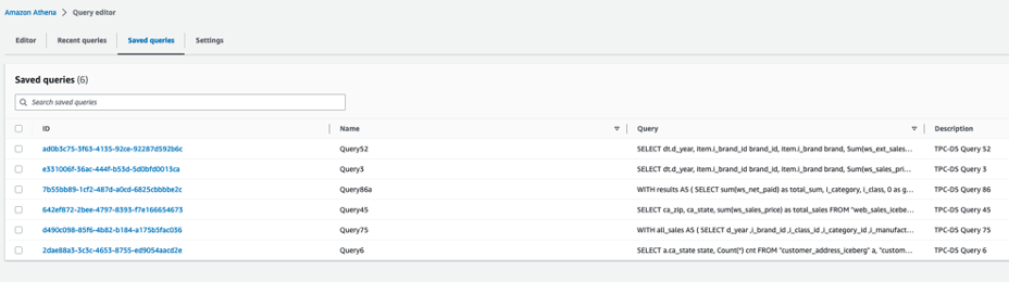 The following queries are listed:
- Query3 – Report the total extended sales price per item brand of a specific manufacturer for all sales in a specific month of the year.
- Query45 – Report the total web sales for customers in specific zip codes, cities, counties, or states, or specific items for a given year and quarter.
- Query52 – Report the total of extended sales price for all items of a specific brand in a specific year and month.
- Query6 – List all the states with at least 10 customers who during a given month bought items with the price tag at least 20% higher than the average price of items in the same category.
- Query75 – For 2 consecutive years, track the sales of items by brand, class, and category.
- Query86a – Roll up the web sales for a given year by category and class, and rank the sales among peers within the parent. For each group, compute the sum of sales and location with the hierarchy and rank within the group.
These queries are examples of queries used in decision-making and reporting in an organization. You can run them in the order you want. For this post, we start with Query3.
- Before you run the query, confirm that Database is set to
datalake.

- Now you can run the query.

- Repeat these steps to run the other queries.
Update the item table
After running the queries, we prepare a batch of updates and inserts of records into the item table.
- First, run the following query to count the number of records in the
itemIceberg table:
This should return 102,000 records.
- Select item records with a price higher than $90:
This will return 1,112 records.
The update-item.py job takes these 1,112 records, modifies 11 records to change the name of the brand to Unknown, and changes the remaining 1,101 records’ i\_item\_id key to flag them as new records. As a result, a batch of 11 updates and 1,101 inserts are merged into the item\_iceberg table.
The 11 records to be updated are those with price higher than $90, and the brand name starts with corpnameless.
- Run the following query:
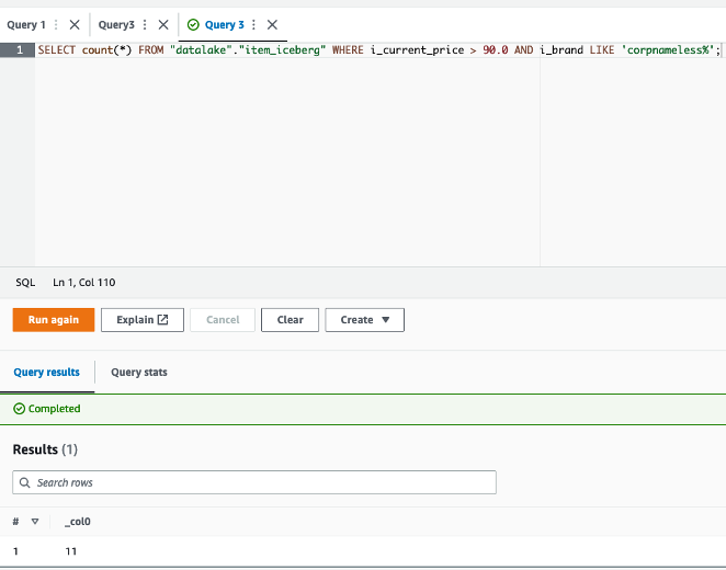
The result is 11 records. The item\_update.py job replaces the brand name with Unknown and merges the batch into the Iceberg table.
Now you can return to the EMR Serverless console and run the job on the EMR Serverless application.
- On the application details page, choose Submit job.
- For Name, enter
update-item-job. - For Runtime role¸ use the same role that you used previously.
- For S3 URI, enter the
update-item.pyscript location.
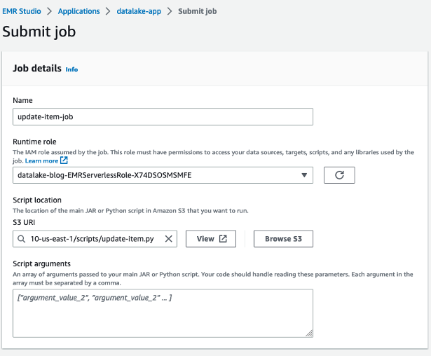
- Under Spark properties, choose Edit in text.
- Enter the following properties, replacing the <BUCKET-NAME> with your own
datalake-<####>-us-east-1:
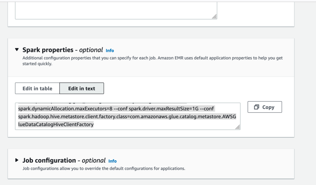
- Then submit the job.

- After the job finishes successfully, return to the Athena console and run the following query:
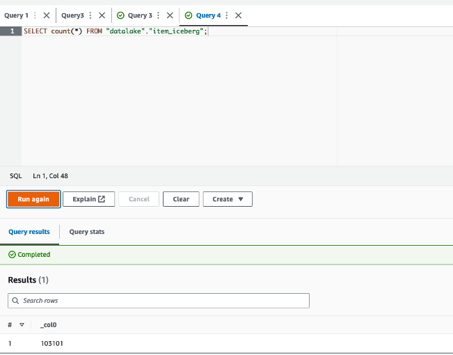
The returned result is 103,101 = 102,000 + (1,112 – 11). The batch was merged successfully.
Time travel
To run a time travel query, complete the following steps:
- Get the timestamp of the job run via the application details page on the EMR Serverless console, or the Spark UI on the History Server, as shown in the following screenshot.
This time could be just minutes before you ran the update Spark job.
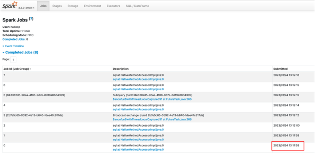
- Convert the timestamp from the format
YYYY/MM/DD hh:mm:ss to YYYY-MM-DDThh:mm:ss.sTZDwith time zone. For example, from2023/02/20 14:40:41to2023-02-20 14:40:41.000 UTC. - On the Athena console, run the following query to count the
itemtable records at a time before the update job, replacing <TRAVEL\_TIME> with your time:
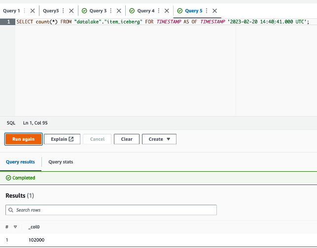
The query will give 102,000 as a result, the expected table size before running the update job.
- Now you can run a query with a timestamp after the successful run of the update job (for example,
2023-02-20 15:06:00.000 UTC):
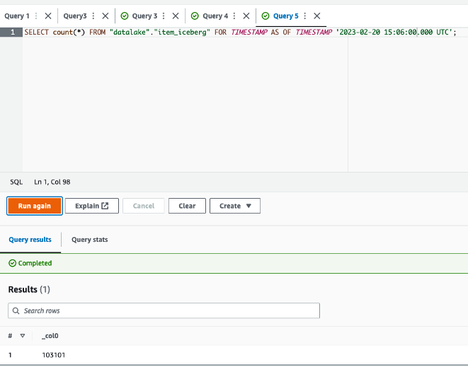
The query will now give 103,101 as the size of the table at that time, after the update job successfully finished.
Additionally, you can query in Athena based on the version ID of a snapshot in Iceberg. However, for more advanced use cases, such as to roll back to a given version or to find version IDs, you can use Iceberg’s SDK or Spark on Amazon EMR.
Clean up
Complete the following steps to clean up your resources:
- On the Amazon S3 console, empty your buckets.
- On the Athena console, delete the workgroup
DatalakeWorkgroup. - On the EMR Studio console, stop the application
datalake-app. - On the AWS CloudFormation console, delete the CloudFormation stack.
Conclusion
In this post, we created a serverless transactional data lake with Iceberg tables, EMR Serverless, and Athena. We used TPC-DS sales data with 10 GB data and more than 7 million records in the fact table. We demonstrated how straightforward it is to rely on SQL and Spark to run serverless jobs for data ingestion and upserts. Moreover, we showed how to run complex BI queries directly on Iceberg tables from Athena for reporting.
You can start building your serverless transactional data lake on AWS today, and dive deep into the features and optimizations Iceberg provides to build analytics applications more easily. Iceberg can also help you in the future to improve performance and reduce costs.
About the Author

Houssem is a Specialist Solutions Architect at AWS with a focus on analytics. He is passionate about data and emerging technologies in analytics. He holds a PhD on data management in the cloud. Prior to joining AWS, he worked on several big data projects and published several research papers in international conferences and venues.
Amazon QuickSight is a fully managed, cloud-native business intelligence (BI) service that makes it easy to connect to your data, create interactive dashboards and reports, and share these with tens of thousands of users, either within QuickSight or embedded in your application or website.
QuickSight recently launched a new major version of its Embedding SDK (v2.0) to improve developer experience when embedding QuickSight in your application or website. The QuickSight SDK v2.0 adds several customization improvements such as an optional preloader and new external hooks for managing undo, redo, print options, and parameters. Additionally, there are major rewrites to deliver developer-focused improvements, including static type checking, enhanced runtime validation, strong consistency in call patterns, and optimized event chaining.
The new SDK supports improved code completion when integrated with IDEs through its adoption of TypeScript and the newly introduced frameOptions and contentOptions, which segment embedding options into parameters unified for all embedding experiences and parameters unique for each embedding experience, respectively. Additionally, SDK v2.0 offers increased visibility by providing new experience-specific information and warnings within the SDK. This increases transparency, and developers can monitor and handle new content states.
The QuickSight SDK v2.0 is modernized by using promises for all actions, so developers can use async and await functions for better event management. Actions are further standardized to return a response for both data requesting and non-data requesting actions, so developers have full visibility to the end-to-end application handshake.
In addition to the new SDK, we are also introducing state persistence for user-based dashboard and console embedding. The GenerateEmbedUrlForRegisteredUser API is updated to support this feature and improves end-user experience and interactivity on embedded content.
SDK Feature overview
The QuickSight SDK v2.0 offers new functionalities along with elevating developers’ experience. The following functionalities have been added in this version:
- Dashboard undo, redo, and reset actions can now be invoked from the application
- A loading animation can be added to the dashboard container while the contents of the dashboard are loaded
- Frame creation, mounting, and failure are communicated as change events that can be used by the application
- Actions
getParameter()values andsetParameter()values are unified, eliminating additional data transformations
Using the new SDK
The embed URL obtained using the GenerateEmbedUrlForRegisteredUser or GenerateEmbedUrlForAnonymousUser APIs can be consumed in the application using the embedDashboard experience in SDK v2.0. This method takes two parameters:
- frameOptions – This is a required parameter, and its properties determine the container options to embed a dashboard:
- url – The embed URL generated using
GenerateEmbedUrlForRegisteredUserorGenerateEmbedUrlForAnonymousUserAPIs - container – The parent
HTMLElementto embed the dashboard
- url – The embed URL generated using
- contentOptions – This is an optional parameter that controls the dashboard locale and captures events from the SDK.
The following sample code uses the preceding parameters to embed a dashboard:
Render a loading animation while the dashboard loads
SDK v2.0 allows an option to render a loading animation in the iFrame container while the dashboard loads. This improves user experience by suggesting resource loading is in progress and where it will appear, and eliminates any perceived latency.
You can enable a loading animation by using the withIframePlaceholder option in the frameOption parameter:
This option is supported by all embedding experiences.
Monitor changes in SDK code status
SDK v2.0 supports a new callback onChange, which returns eventNames along with corresponding eventCodes to indicate errors, warnings, or information from the SDK.
You can use the events returned by the callback to monitor frame creation status and code status returned by the SDK. For example, if the SDK returns an error when an invalid embed URL is used, you can use a placeholder text or image in place of the embedded experience to notify the user.
The following eventNames and eventCodes are returned as part of the onChange callback when there is a change in the SDK code status.
| eventName | eventCode |
| ERROR | FRAME\_NOT\_CREATED: Invoked when the creation of the iframe element failed |
NO\_BODY: Invoked when there is no body element in the hosting HTML | |
NO\_CONTAINER: Invoked when the experience container is not found | |
NO\_URL: Invoked when no URL is provided in the frameOptions | |
INVALID\_URL: Invoked when the URL provided is not a valid URL for the experience | |
| INFO | FRAME\_STARTED: Invoked just before the iframe is created |
FRAME\_MOUNTED: Invoked after the iframe is appended into the experience container | |
FRAME\_LOADED: Invoked after the iframe element emitted the load event | |
| WARN | UNRECOGNIZED\_CONTENT\_OPTIONS: Invoked when the content options for the experience contain unrecognized properties |
UNRECOGNIZED\_EVENT\_TARGET: Invoked when a message with an unrecognized event target is received |
See the following code:
Monitor interactions in embedded dashboards
Another callback supported by SDK v2.0 is onMessage, which returns information about specific events within an embedded experience. The eventName returned depends on the type of embedding experience used and allows application developers to invoke custom code for specific events.
For example, you can monitor if an embedded dashboard is fully loaded or invoke a custom function that logs the parameter values end-users set or change within the dashboard. Your application can now work seamlessly with SDK v2.0 to track and react to interactions within an embedded experience.
The eventNames returned are specific to the embedding experience used. The following eventNames are for the dashboard embedding experience. For additional eventNames, visit the GitHub repo.
CONTENT\_LOADEDERROR\_OCCURREDPARAMETERS\_CHANGEDSELECTED\_SHEET\_CHANGEDSIZE\_CHANGEDMODAL\_OPENED
See the following code:
Initiate dashboard print from the application
The new SDK version supports initiating undo, redo, reset, and print from the parent application, without having to add the native embedded QuickSight navbar. This allows developers flexibility to add custom buttons or application logic to control and invoke these options.
For example, you can add a standalone button in your application that allows end-users to print an embedded dashboard, without showing a print icon or navbar within the embedded frame. This can be done using the initiatePrint action:
The following code sample shows a loading animation, SDK code status, and dashboard interaction monitoring, along with initiating dashboard print from the application:
State persistence
In addition to the new SDK, QuickSight now supports state persistence for dashboard and console embedding. State Persistance means when readers slice and dice embedded dashboards with filters, QuickSight will persist filter selection until they return to the dashboard. Readers can pick up where they left off and don’t have to re-select filters.
State persistence is currently supported only for the user-based (not anonymous) dashboard and console embedding experience.
You can enable state persistence using the FeatureConfigurations parameter in the GenerateEmbedUrlForRegisteredUser API. FeatureConfigurations contains StatePersistence structure that can be customized by setting Enabled as true or false.
The API structure is below:
The following code disables state persistence for QuickSight console embedding:
Considerations
Note the following when using these features:
- For dashboard embedding, state persistence is disabled by default. To enable this feature, set
Enabledparameter inStatePersistenceto true. - For console embedding, state persistence is enabled by default. To disable this feature, set
Enabledparameter inStatePersistenceto false.
Conclusion
With the latest iteration of the QuickSight Embedding SDK, you can indicate when an embedded experience is loading, monitor and respond to errors from the SDK, observe changes and interactivity, along with invoking undo, redo, reset, and print actions from application code.
Additionally, you can enable state persistence to persist filter selection for readers and allow them to pick up where they left off when revisiting an embedded dashboard.
For more detailed information about the SDK and experience-specific options, visit the GitHub repo.
About the authors
 Raj Jayaraman is a Senior Specialist Solutions Architect for Amazon QuickSight. Raj focuses on helping customers develop sample dashboards, embed analytics and adopt BI design patterns and best practices.
Mayank Agarwal is a product manager for Amazon QuickSight, AWS’ cloud-native, fully managed BI service. He focuses on account administration, governance and developer experience. He started his career as an embedded software engineer developing handheld devices. Prior to QuickSight he was leading engineering teams at Credence ID, developing custom mobile embedded device and web solutions using AWS services that make biometric enrollment and identification fast, intuitive, and cost-effective for Government sector, healthcare and transaction security applications.
 Rohit Pujari is the Head of Product for Embedded Analytics at QuickSight. He is passionate about shaping the future of infusing data-rich experiences into products and applications we use every day. Rohit brings a wealth of experience in analytics and machine learning from having worked with leading data companies, and their customers. During his free time, you can find him lining up at the local ice cream shop for his second scoop.
Thousands of customers rely on Amazon Redshift to build data warehouses to accelerate time to insights with fast, simple, and secure analytics at scale and analyze data from terabytes to petabytes by running complex analytical queries. Organizations create data marts, which are subsets of the data warehouse and usually oriented for gaining analytical insights specific to a business unit or team. The star schema is a popular data model for building data marts.
In this post, we show how to simplify data loading into a Type 2 slowly changing dimension in Amazon Redshift.
Star schema and slowly changing dimension overview
A star schema is the simplest type of dimensional model, in which the center of the star can have one fact table and a number of associated dimension tables. A dimension is a structure that captures reference data along with associated hierarchies, while a fact table captures different values and metrics that can be aggregated by dimensions. Dimensions provide answers to exploratory business questions by allowing end-users to slice and dice data in a variety of ways using familiar SQL commands.
Whereas operational source systems contain only the latest version of master data, the star schema enables time travel queries to reproduce dimension attribute values on past dates when the fact transaction or event actually happened. The star schema data model allows analytical users to query historical data tying metrics to corresponding dimensional attribute values over time. Time travel is possible because dimension tables contain the exact version of the associated attributes at different time ranges. Relative to the metrics data that keeps changing on a daily or even hourly basis, the dimension attributes change less frequently. Therefore, dimensions in a star schema that keeps track of changes over time are referred to as slowly changing dimensions (SCDs).
Data loading is one of the key aspects of maintaining a data warehouse. In a star schema data model, the central fact table is dependent on the surrounding dimension tables. This is captured in the form of primary key-foreign key relationships, where the dimension table primary keys are referred by foreign keys in the fact table. In the case of Amazon Redshift, uniqueness, primary key, and foreign key constraints are not enforced. However, declaring them will help the optimizer arrive at optimal query plans, provided that the data loading processes enforce their integrity. As part of data loading, the dimension tables, including SCD tables, get loaded first, followed by the fact tables.
SCD population challenge
Populating an SCD dimension table involves merging data from multiple source tables, which are usually normalized. SCD tables contain a pair of date columns (effective and expiry dates) that represent the record’s validity date range. Changes are inserted as new active records effective from the date of data loading, while simultaneously expiring the current active record on a previous day. During each data load, incoming change records are matched against existing active records, comparing each attribute value to determine whether existing records have changed or were deleted or are new records coming in.
In this post, we demonstrate how to simplify data loading into a dimension table with the following methods:
- Using Amazon Simple Storage Service (Amazon S3) to host the initial and incremental data files from source system tables
- Accessing S3 objects using Amazon Redshift Spectrum to carry out data processing to load native tables within Amazon Redshift
- Creating views with window functions to replicate the source system version of each table within Amazon Redshift
- Joining source table views to project attributes matching with dimension table schema
- Applying incremental data to the dimension table, bringing it up to date with source-side changes
Solution overview
In a real-world scenario, records from source system tables are ingested on a periodic basis to an Amazon S3 location before being loaded into star schema tables in Amazon Redshift.
For this demonstration, data from two source tables, customer\_master and customer\_address, are combined to populate the target dimension table dim\_customer, which is the customer dimension table.
The source tables customer\_master and customer\_address share the same primary key, customer\_id, and will be joined on the same to fetch one record per customer\_id along with attributes from both tables. row\_audit\_ts contains the latest timestamp at which the particular source record was inserted or last updated. This column helps identify the change records since the last data extraction.
rec\_source\_status is an optional column that indicates if the corresponding source record was inserted, updated, or deleted. This is applicable in cases where the source system itself provides the changes and populates rec\_source\_status appropriately.
The following figure provides the schema of the source and target tables.

Let’s look closer at the schema of the target table, dim\_customer. It contains different categories of columns:
- Keys – It contains two types of keys:
customer\_skis the primary key of this table. It is also called the surrogate key and has a unique value that is monotonically increasing.customer\_idis the source primary key and provides a reference back to the source system record.
- SCD2 metadata –
rec\_eff\_dtandrec\_exp\_dtindicate the state of the record. These two columns together define the validity of the record. The value inrec\_exp\_dtwill be set as‘9999-12-31’for presently active records. - Attributes – Includes
first\_name,last\_name,employer\_name,email\_id,city, andcountry.
Data loading into a SCD table involves a first-time bulk data loading, referred to as the initial data load. This is followed by continuous or regular data loading, referred to as an incremental data load, to keep the records up to date with changes in the source tables.
To demonstrate the solution, we walk through the following steps for initial data load (1–7) and incremental data load (8–12):
- Land the source data files in an Amazon S3 location, using one subfolder per source table.
- Use an AWS Glue crawler to parse the data files and register tables in the AWS Glue Data Catalog.
- Create an external schema in Amazon Redshift to point to the AWS Glue database containing these tables.
- In Amazon Redshift, create one view per source table to fetch the latest version of the record for each primary key (
customer\_id) value. - Create the
dim\_customertable in Amazon Redshift, which contains attributes from all relevant source tables. - Create a view in Amazon Redshift joining the source table views from Step 4 to project the attributes modeled in the dimension table.
- Populate the initial data from the view created in Step 6 into the
dim\_customertable, generatingcustomer\_sk. - Land the incremental data files for each source table in their respective Amazon S3 location.
- In Amazon Redshift, create a temporary table to accommodate the change-only records.
- Join the view from Step 6 and
dim\_customerand identify change records comparing the combined hash value of attributes. Populate the change records into the temporary table with anI,U, orDindicator. - Update
rec\_exp\_dtindim\_customerfor allUandDrecords from the temporary table. - Insert records into
dim\_customer, querying allIandUrecords from the temporary table.
Prerequisites
Before you get started, make sure you meet the following prerequisites:
- Have an AWS account.
- Create an S3 bucket where the data files that will be loaded into Amazon Redshift are stored.
- Create an Amazon Redshift cluster or endpoint. For instructions, refer to Getting started with Amazon Redshift.
- When your environment is ready, open Amazon Redshift Query Editor v2.0 (see the following screenshot) and connect to your Amazon Redshift cluster or endpoint.

Land data from source tables
Create separate subfolders for each source table in an S3 bucket and place the initial data files within the respective subfolder. In the following image, the initial data files for customer\_master and customer\_address are made available within two different subfolders. To try out the solution, you can use customer\_master\_with\_ts.csv and customer\_address\_with\_ts.csv as initial data files.

It’s important to include an audit timestamp (row\_audit\_ts) column that indicates when each record was inserted or last updated. As part of incremental data loading, rows with the same primary key value (customer\_id) can arrive more than once. The row\_audit\_ts column helps identify the latest version of such records for a given customer\_id to be used for further processing.
Register source tables in the AWS Glue Data Catalog
We use an AWS Glue crawler to infer metadata from delimited data files like the CSV files used in this post. For instructions on getting started with an AWS Glue crawler, refer to Tutorial: Adding an AWS Glue crawler.
Create an AWS Glue crawler and point it to the Amazon S3 location that contains the source table subfolders, within which the associated data files are placed. When you’re creating the AWS Glue crawler, create a new database named rs-dimension-blog. The following screenshots show the AWS Glue crawler configuration chosen for our data files.


Note that for the Set output and scheduling section, the advanced options are left unchanged.

Running this crawler should create the following tables within the rs-dimension-blog database:
customer\_addresscustomer\_master
Create schemas in Amazon Redshift
First, create an AWS Identity and Access Management (IAM) role named rs-dim-blog-spectrum-role. For instructions, refer to Create an IAM role for Amazon Redshift.
The IAM role has Amazon Redshift as the trusted entity, and the permissions policy includes AmazonS3ReadOnlyAccess and AWSGlueConsoleFullAccess, because we’re using the AWS Glue Data Catalog. Then associate the IAM role with the Amazon Redshift cluster or endpoint.
Instead, you can also set the IAM role as the default for your Amazon Redshift cluster or endpoint. If you do so, in the following create external schema command, pass the iam\_role parameter as iam\_role default.
Now, open Amazon Redshift Query Editor V2 and create an external schema passing the newly created IAM role and specifying the database as rs-dimension-blog. The database name rs-dimension-blog is the one created in the Data Catalog as part of configuring the crawler in the preceding section. See the following code:
Check if the tables registered in the Data Catalog in the preceding section are visible from within Amazon Redshift:
Each of these queries will return 10 rows from the respective Data Catalog tables.
Create another schema in Amazon Redshift to host the table, dim\_customer:
Create views to fetch the latest records from each source table
Create a view for the customer\_master table, naming it vw\_cust\_mstr\_latest:
The preceding query uses row\_number, which is a window function provided by Amazon Redshift. Using window functions enables you to create analytic business queries more efficiently. Window functions operate on a partition of a result set, and return a value for every row in that window. The row\_number window function determines the ordinal number of the current row within a group of rows, counting from 1, based on the ORDER BY expression in the OVER clause. By including the PARTITION BY clause as customer\_id, groups are created for each value of customer\_id and ordinal numbers are reset for each group.
Create a view for the customer\_address table, naming it vw\_cust\_addr\_latest:
Both view definitions use the row\_number window function of Amazon Redshift, ordering the records by descending order of the row\_audit\_ts column (the audit timestamp column). The condition rnum=1 fetches the latest record for each customer\_id value.
Create the dim\_customer table in Amazon Redshift
Create dim\_customer as an internal table in Amazon Redshift within the rs\_dim\_blog schema. The dimension table includes the column customer\_sk, that acts as the surrogate key column and enables us to capture a time-sensitive version of each customer record. The validity period for each record is defined by the columns rec\_eff\_dt and rec\_exp\_dt, representing record effective date and record expiry date, respectively. See the following code:
Create a view to consolidate the latest version of source records
Create the view vw\_dim\_customer\_src, which consolidates the latest records from both source tables using left outer join, keeping them ready to be populated into the Amazon Redshift dimension table. This view fetches data from the latest views defined in the section “Create views to fetch the latest records from each source table”:
At this point, this view fetches the initial data for loading into the dim\_customer table that we are about to create. In your use-case, use a similar approach to create and join the required source table views to populate your target dimension table.
Populate initial data into dim\_customer
Populate the initial data into the dim\_customer table by querying the view vw\_dim\_customer\_src. Because this is the initial data load, running row numbers generated by the row\_number window function will suffice to populate a unique value in the customer\_sk column starting from 1:
In this query, we have specified ’2022-07-01’ as the value in rec\_eff\_dt for all initial data records. For your use-case, you can modify this date value as appropriate to your situation.
The preceding steps complete the initial data loading into the dim\_customer table. In the next steps, we proceed with populating incremental data.
Land ongoing change data files in Amazon S3
After the initial load, the source systems provide data files on an ongoing basis, either containing only new and change records or a full extract containing all records for a particular table.
You can use the sample files customer\_master\_with\_ts\_incr.csv and customer\_address\_with\_ts\_incr.csv, which contain changed as well as new records. These incremental files need to be placed in the same location in Amazon S3 where the initial data files were placed. Please see section “Land data from source tables”. This will result in the corresponding Redshift Spectrum tables automatically reading the additional rows.
If you used the sample file for customer\_master, after adding the incremental files, the following query shows the initial as well as incremental records:

In case of full extracts, we can identify deletes occurring in the source system tables by comparing the previous and current versions and looking for missing records. In case of change-only extracts where the rec\_source\_status column is present, its value will help us identify deleted records. In either case, land the ongoing change data files in the respective Amazon S3 locations.
For this example, we have uploaded the incremental data for the customer\_master and customer\_address source tables with a few customer\_id records receiving updates and a few new records being added.
Create a temporary table to capture change records
Create the temporary table temp\_dim\_customer to store all changes that need to be applied to the target dim\_customer table:
Populate the temporary table with new and changed records
This is a multi-step process that can be combined into a single complex SQL. Complete the following steps:
- Fetch the latest version of all customer attributes by querying the view
vw\_dim\_customer\_src:
Amazon Redshift offers hashing functions such as sha2, which converts a variable length string input into a fixed length character output. The output string is a text representation of the hexadecimal value of the checksum with the specified number of bits. In this case, we pass a concatenated set of customer attributes whose change we want to track, specifying the number of bits as 512. We’ll use the output of the hash function to determine if any of the attributes have undergone a change. This dataset will be called newver (new version).
Because we landed the ongoing change data in the same location as the initial data files, the records retrieved from the preceding query (in newver) include all records, even the unchanged ones. But because of the definition of the view vw\_dim\_customer\_src, we get only one record per customerid, which is its latest version based on row\_audit\_ts.
- In a similar manner, retrieve the latest version of all customer records from
dim\_customer, which are identified byrec\_exp\_dt=‘9999-12-31’. While doing so, also retrieve thesha2value of all customer attributes available indim\_customer:
This dataset will be called oldver (old or existing version).
- Identify the current maximum surrogate key value from the
dim\_customertable:
This value (maxval) will be added to the row\_number before being used as the customer\_sk value for the change records that need to be inserted.
- Perform a full outer join of the old version of records (
oldver) and the new version (newver) of records on thecustomer\_idcolumn. Then compare the old and new hash values generated by thesha2function to determine if the change record is an insert, update, or delete:
We tag the records as follows:
- If the
customer\_idis non-existent in theoldverdataset (oldver.customer\_id is null), it’s tagged as an insert (‘I'). - Otherwise, if the
customer\_idis non-existent in thenewverdataset (newver.customer\_id is null), it’s tagged as a delete (‘D'). - Otherwise, if the old
hash\_valueand newhash\_valueare different, these records represent an update (‘U'). - Otherwise, it indicates that the record has not undergone any change and therefore can be ignored or marked as not-to-be-processed (
‘N').
Make sure to modify the preceding logic if the source extract contains rec\_source\_status to identify deleted records.
Although sha2 output maps a possibly infinite set of input strings to a finite set of output strings, the chances of collision of hash values for the original row values and changed row values are very unlikely. Instead of individually comparing each column value before and after, we compare the hash values generated by sha2 to conclude if there has been a change in any of the attributes of the customer record. For your use-case, we recommend you choose a hash function that works for your data conditions after adequate testing. Instead, you can compare individual column values if none of the hash functions satisfactorily meet your expectations.
- Combining the outputs from the preceding steps, let’s create the INSERT statement that captures only change records to populate the temporary table:
Expire updated customer records
With the temp\_dim\_customer table now containing only the change records (either ‘I’, ‘U’, or ‘D’), the same can be applied on the target dim\_customer table.
Let’s first fetch all records with values ‘U’ or ‘D’ in the iud\_op column. These are records that have either been deleted or updated in the source system. Because dim\_customer is a slowly changing dimension, it needs to reflect the validity period of each customer record. In this case, we expire the presently active recorts that have been updated or deleted. We expire these records as of yesterday (by setting rec\_exp\_dt=current\_date-1) matching on the customer\_id column:
Insert new and changed records
As the last step, we need to insert the newer version of updated records along with all first-time inserts. These are indicated by ‘U’ and ‘I’, respectively, in the iud\_op column in the temp\_dim\_customer table:
Depending on the SQL client setting, you might want to run a commit transaction; command to verify that the preceding changes are persisted successfully in Amazon Redshift.
Check the final output
You can run the following query and see that the dim\_customer table now contains both the initial data records plus the incremental data records, capturing multiple versions for those customer\_id values that got changed as part of incremental data loading. The output also indicates that each record has been populated with appropriate values in rec\_eff\_dt and rec\_exp\_dt corresponding to the record validity period.
For the sample data files provided in this article, the preceding query returns the following records. If you’re using the sample data files provided in this post, note that the values in customer\_sk may not match with what is shown in the following table.

In this post, we only show the important SQL statements; the complete SQL code is available in load\_scd2\_sample\_dim\_customer.sql.
Clean up
If you no longer need the resources you created, you can delete them to prevent incurring additional charges.
Conclusion
In this post, you learned how to simplify data loading into Type-2 SCD tables in Amazon Redshift, covering both initial data loading and incremental data loading. The approach deals with multiple source tables populating a target dimension table, capturing the latest version of source records as of each run.
Refer to Amazon Redshift data loading best practices for further materials and additional best practices, and see Updating and inserting new data for instructions to implement updates and inserts.
About the Author
 Vaidy Kalpathy is a Senior Data Lab Solution Architect at AWS, where he helps customers modernize their data platform and defines end to end data strategy including data ingestion, transformation, security, visualization. He is passionate about working backwards from business use cases, creating scalable and custom fit architectures to help customers innovate using data analytics services on AWS.
The value of data is time sensitive. Real-time processing makes data-driven decisions accurate and actionable in seconds or minutes instead of hours or days. Change data capture (CDC) refers to the process of identifying and capturing changes made to data in a database and then delivering those changes in real time to a downstream system. Capturing every change from transactions in a source database and moving them to the target in real time keeps the systems synchronized, and helps with real-time analytics use cases and zero-downtime database migrations. The following are a few benefits of CDC:
- It eliminates the need for bulk load updating and inconvenient batch windows by enabling incremental loading or real-time streaming of data changes into your target repository.
- It ensures that data in multiple systems stays in sync. This is especially important if you’re making time-sensitive decisions in a high-velocity data environment.
Kafka Connect is an open-source component of Apache Kafka that works as a centralized data hub for simple data integration between databases, key-value stores, search indexes, and file systems. The AWS Glue Schema Registry allows you to centrally discover, control, and evolve data stream schemas. Kafka Connect and Schema Registry integrate to capture schema information from connectors. Kafka Connect provides a mechanism for converting data from the internal data types used by Kafka Connect to data types represented as Avro, Protobuf, or JSON Schema. AvroConverter, ProtobufConverter, and JsonSchemaConverter automatically register schemas generated by Kafka connectors (source) that produce data to Kafka. Connectors (sink) that consume data from Kafka receive schema information in addition to the data for each message. This allows sink connectors to know the structure of the data to provide capabilities like maintaining a database table schema in a data catalog.
The post demonstrates how to build an end-to-end CDC using Amazon MSK Connect, an AWS managed service to deploy and run Kafka Connect applications and AWS Glue Schema Registry, which allows you to centrally discover, control, and evolve data stream schemas.
Solution overview

On the producer side, for this example we choose a MySQL-compatible Amazon Aurora database as the data source, and we have a Debezium MySQL connector to perform CDC. The Debezium connector continuously monitors the databases and pushes row-level changes to a Kafka topic. The connector fetches the schema from the database to serialize the records into a binary form. If the schema doesn’t already exist in the registry, the schema will be registered. If the schema exists but the serializer is using a new version, the schema registry checks the compatibility mode of the schema before updating the schema. In this solution, we use backward compatibility mode. The schema registry returns an error if a new version of the schema is not backward compatible, and we can configure Kafka Connect to send incompatible messages to the dead-letter queue.
On the consumer side, we use an Amazon Simple Storage Service (Amazon S3) sink connector to deserialize the record and store changes to Amazon S3. We build and deploy the Debezium connector and the Amazon S3 sink using MSK Connect.
Example schema
For this post, we use the following schema as the first version of the table:
Prerequisites
Before configuring the MSK producer and consumer connectors, we need to first set up a data source, MSK cluster, and new schema registry. We provide an AWS CloudFormation template to generate the supporting resources needed for the solution:
- A MySQL-compatible Aurora database as the data source. To perform CDC, we turn on binary logging in the DB cluster parameter group.
- An MSK cluster. To simplify the network connection, we use the same VPC for the Aurora database and the MSK cluster.
- Two schema registries to handle schemas for message key and message value.
- One S3 bucket as the data sink.
- MSK Connect plugins and worker configuration needed for this demo.
- One Amazon Elastic Compute Cloud (Amazon EC2) instance to run database commands.
To set up resources in your AWS account, complete the following steps in an AWS Region that supports Amazon MSK, MSK Connect, and the AWS Glue Schema Registry:
- Choose Launch Stack:

- Choose Next.
- For Stack name, enter suitable name.
- For Database Password, enter the password you want for the database user.
- Keep other values as default.
- Choose Next.
- On the next page, choose Next.
- Review the details on the final page and select I acknowledge that AWS CloudFormation might create IAM resources.
- Choose Create stack.
Custom plugin for the source and destination connector
A custom plugin is a set of JAR files that contain the implementation of one or more connectors, transforms, or converters. Amazon MSK will install the plugin on the workers of the MSK Connect cluster where the connector is running. As part of this demo, for the source connector we use open-source Debezium MySQL connector JARs, and for the destination connector we use the Confluent community licensed Amazon S3 sink connector JARs. Both the plugins are also added with libraries for Avro Serializers and Deserializers of the AWS Glue Schema Registry. These custom plugins are already created as part of the CloudFormation template deployed in the previous step.
Use the AWS Glue Schema Registry with the Debezium connector on MSK Connect as the MSK producer
We first deploy the source connector using the Debezium MySQL plugin to stream data from an Amazon Aurora MySQL-Compatible Edition database to Amazon MSK. Complete the following steps:
- On the Amazon MSK console, in the navigation pane, under MSK Connect, choose Connectors.
- Choose Create connector.
- Choose Use existing custom plugin and then pick the custom plugin with name starting
msk-blog-debezium-source-plugin. - Choose Next.
- Enter a suitable name like
debezium-mysql-connectorand an optional description. - For Apache Kafka cluster, choose MSK cluster and choose the cluster created by the CloudFormation template.
- In Connector configuration, delete the default values and use the following configuration key-value pairs and with the appropriate values:
- name – The name used for the connector.
- database.hostsname – The CloudFormation output for Database Endpoint.
- database.user and database.password – The parameters passed in the CloudFormation template.
- database.history.kafka.bootstrap.servers – The CloudFormation output for Kafka Bootstrap.
- key.converter.region and value.converter.region – Your Region.
Some of these settings are generic and should be specified for any connector. For example:
- connector.class is the Java class of the connector
- tasks.max is the maximum number of tasks that should be created for this connector
Some settings (database.*, transforms.*) are specific to the Debezium MySQL connector. Refer to Debezium MySQL Source Connector Configuration Properties for more information.
Some settings (key.converter.* and value.converter.*) are specific to the Schema Registry. We use the AWSKafkaAvroConverter from the AWS Glue Schema Registry Library as the format converter. To configure AWSKafkaAvroConverter, we use the value of the string constant properties in the AWSSchemaRegistryConstants class:
key.converterandvalue.convertercontrol the format of the data that will be written to Kafka for source connectors or read from Kafka for sink connectors. We useAWSKafkaAvroConverterfor Avro format.key.converter.registry.nameandvalue.converter.registry.namedefine which schema registry to use.key.converter.compatibilityandvalue.converter.compatibilitydefine the compatibility model.
Refer to Using Kafka Connect with AWS Glue Schema Registry for more information.
- Next, we configure Connector capacity. We can choose Provisioned and leave other properties as default
- For Worker configuration, choose the custom worker configuration with name starting
msk-gsr-blogcreated as part of the CloudFormation template. - For Access permissions, use the AWS Identity and Access Management (IAM) role generated by the CloudFormation template
MSKConnectRole. - Choose Next.
- For Security, choose the defaults.
- Choose Next.
- For Log delivery, select Deliver to Amazon CloudWatch Logs and browse for the log group created by the CloudFormation template (
msk-connector-logs). - Choose Next.
- Review the settings and choose Create connector.
After a few minutes, the connector changes to running status.
Use the AWS Glue Schema Registry with the Confluent S3 sink connector running on MSK Connect as the MSK consumer
We deploy the sink connector using the Confluent S3 sink plugin to stream data from Amazon MSK to Amazon S3. Complete the following steps:
-
- On the Amazon MSK console, in the navigation pane, under MSK Connect, choose Connectors.
- Choose Create connector.
- Choose Use existing custom plugin and choose the custom plugin with name starting
msk-blog-S3sink-plugin. - Choose Next.
- Enter a suitable name like
s3-sink-connectorand an optional description. - For Apache Kafka cluster, choose MSK cluster and select the cluster created by the CloudFormation template.
- In Connector configuration, delete the default values provided and use the following configuration key-value pairs with appropriate values:
-
- name – The same name used for the connector.
- s3.bucket.name – The CloudFormation output for Bucket Name.
- s3.region, key.converter.region, and value.converter.region – Your Region.
-
- Next, we configure Connector capacity. We can choose Provisioned and leave other properties as default
- For Worker configuration, choose the custom worker configuration with name starting
msk-gsr-blogcreated as part of the CloudFormation template. - For Access permissions, use the IAM role generated by the CloudFormation template
MSKConnectRole. - Choose Next.
- For Security, choose the defaults.
- Choose Next.
- For Log delivery, select Deliver to Amazon CloudWatch Logs and browse for the log group created by the CloudFormation template
msk-connector-logs. - Choose Next.
- Review the settings and choose Create connector.
After a few minutes, the connector is running.
Test the end-to-end CDC log stream
Now that both the Debezium and S3 sink connectors are up and running, complete the following steps to test the end-to-end CDC:
- On the Amazon EC2 console, navigate to the Security groups page.
- Select the security group
ClientInstanceSecurityGroupand choose Edit inbound rules. - Add an inbound rule allowing SSH connection from your local network.
- On the Instances page, select the instance
ClientInstanceand choose Connect. - On the EC2 Instance Connect tab, choose Connect.
- Ensure your current working directory is
/home/ec2-userand it has the filescreate\_table.sql,alter\_table.sql,initial\_insert.sql, andinsert\_data\_with\_new\_column.sql. - Create a table in your MySQL database by running the following command (provide the database host name from the CloudFormation template outputs):
- When prompted for a password, enter the password from the CloudFormation template parameters.
- Insert some sample data into the table with the following command:
- When prompted for a password, enter the password from the CloudFormation template parameters.
- On the AWS Glue console, choose Schema registries in the navigation pane, then choose Schemas.
- Navigate to
db1.sampledatabase.moviesversion 1 to check the new schema created for the movies table:
A separate S3 folder is created for each partition of the Kafka topic, and data for the topic is written in that folder.
- On the Amazon S3 console, check for data written in Parquet format in the folder for your Kafka topic.
Schema evolution
After the initial schema is defined, applications may need to evolve it over time. When this happens, it’s critical for the downstream consumers to be able to handle data encoded with both the old and the new schema seamlessly. Compatibility modes allow you to control how schemas can or can’t evolve over time. These modes form the contract between applications producing and consuming data. For detailed information about different compatibility modes available in the AWS Glue Schema Registry, refer to AWS Glue Schema Registry. In our example, we use backward combability to ensure consumers can read both the current and previous schema versions. Complete the following steps:
- Add a new column to the table by running the following command:
- Insert new data into the table by running the following command:
- On the AWS Glue console, choose Schema registries in the navigation pane, then choose Schemas.
- Navigate to the schema
db1.sampledatabase.moviesversion 2 to check the new version of the schema created for the movies table movies including the country column that you added:
- On the Amazon S3 console, check for data written in Parquet format in the folder for the Kafka topic.
Clean up
To help prevent unwanted charges to your AWS account, delete the AWS resources that you used in this post:
- On the Amazon S3 console, navigate to the S3 bucket created by the CloudFormation template.
- Select all files and folders and choose Delete.
- Enter permanently delete as directed and choose Delete objects.
- On the AWS CloudFormation console, delete the stack you created.
- Wait for the stack status to change to DELETE\_COMPLETE.
Conclusion
This post demonstrated how to use Amazon MSK, MSK Connect, and the AWS Glue Schema Registry to build a CDC log stream and evolve schemas for data streams as business needs change. You can apply this architecture pattern to other data sources with different Kafka connecters. For more information, refer to the MSK Connect examples.
About the Author
 Kalyan Janaki is Senior Big Data & Analytics Specialist with Amazon Web Services. He helps customers architect and build highly scalable, performant, and secure cloud-based solutions on AWS.
This post provides guidance on how to build scalable analytical solutions for gaming industry use cases using Amazon Redshift Serverless. It covers how to use a conceptual, logical architecture for some of the most popular gaming industry use cases like event analysis, in-game purchase recommendations, measuring player satisfaction, telemetry data analysis, and more. This post also discusses the art of the possible with newer innovations in AWS services around streaming, machine learning (ML), data sharing, and serverless capabilities.
Our gaming customers tell us that their key business objectives include the following:
- Increased revenue from in-app purchases
- High average revenue per user and lifetime value
- Improved stickiness with better gaming experience
- Improved event productivity and high ROI
Our gaming customers also tell us that while building analytics solutions, they want the following:
- Low-code or no-code model – Out-of-the-box solutions are preferred to building customized solutions.
- Decoupled and scalable – Serverless, auto scaled, and fully managed services are preferred over manually managed services. Each service should be easily replaceable, enhanced with little or no dependency. Solutions should be flexible to scale up and down.
- Portability to multiple channels – Solutions should be compatible with most of endpoint channels like PC, mobile, and gaming platforms.
- Flexible and easy to use – The solutions should provide less restrictive, easy-to-access, and ready-to-use data. They should also provide optimal performance with low or no tuning.
Analytics reference architecture for gaming organizations
In this section, we discuss how gaming organizations can use a data hub architecture to address the analytical needs of an enterprise, which requires the same data at multiple levels of granularity and different formats, and is standardized for faster consumption. A data hub is a center of data exchange that constitutes a hub of data repositories and is supported by data engineering, data governance, security, and monitoring services.
A data hub contains data at multiple levels of granularity and is often not integrated. It differs from a data lake by offering data that is pre-validated and standardized, allowing for simpler consumption by users. Data hubs and data lakes can coexist in an organization, complementing each other. Data hubs are more focused around enabling businesses to consume standardized data quickly and easily. Data lakes are more focused around storing and maintaining all the data in an organization in one place. And unlike data warehouses, which are primarily analytical stores, a data hub is a combination of all types of repositories—analytical, transactional, operational, reference, and data I/O services, along with governance processes. A data warehouse is one of the components in a data hub.
The following diagram is a conceptual analytics data hub reference architecture. This architecture resembles a hub-and-spoke approach. Data repositories represent the hub. External processes are the spokes feeding data to and from the hub. This reference architecture partly combines a data hub and data lake to enable comprehensive analytics services.
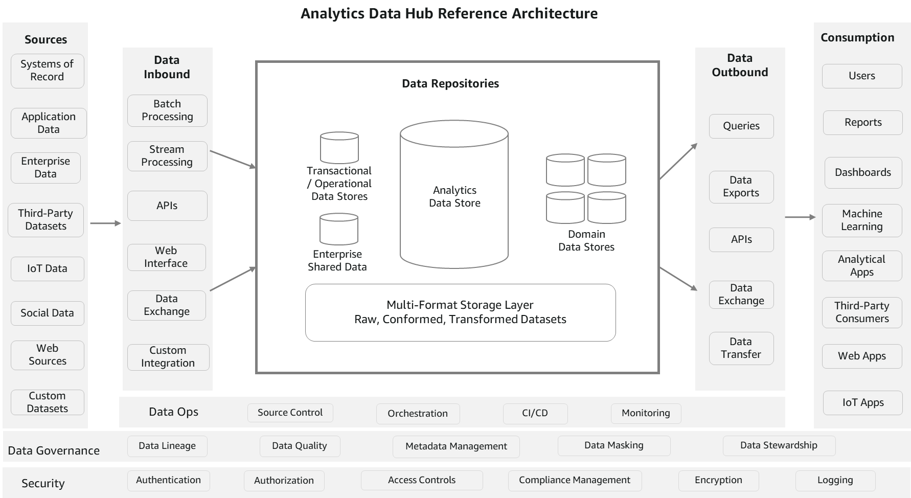
Let’s look at the components of the architecture in more detail.
Sources
Data can be loaded from multiple sources, such as systems of record, data generated from applications, operational data stores, enterprise-wide reference data and metadata, data from vendors and partners, machine-generated data, social sources, and web sources. The source data is usually in either structured or semi-structured formats, which are highly and loosely formatted, respectively.
Data inbound
This section consists of components to process and load the data from multiple sources into data repositories. It can be in batch mode, continuous, pub/sub, or any other
custom integration. ETL (extract, transform, and load) technologies, streaming services, APIs, and data exchange interfaces are the core components of this pillar. Unlike ingestion processes, data can be transformed as per business rules before loading. You can apply technical or business data quality rules and load raw data as well. Essentially, it provides the flexibility to get the data into repositories in its most usable form.
Data repositories
This section consists of a group of data stores, which includes data warehouses, transactional or operational data stores, reference data stores, domain data stores housing purpose-built business views, and enterprise datasets (file storage). The file storage component is usually a common component between a data hub and a data lake to avoid data duplication and provide comprehensiveness. Data can also be shared among all these repositories without physically moving with features, such as data sharing and federated queries. However, data copy and duplication are allowed considering various consumption needs in terms of formats and latency.
Data outbound
Data is often consumed using structured queries for analytical needs. Also, datasets are accessed for ML, data exporting, and publishing needs. This section consists of components to query the data, export, exchange, and APIs. In terms of implementation, the same technologies may be used for both inbound and outbound, but the functions are different. However, it’s not mandatory to use the same technologies. These processes aren’t transformation heavy because the data is already standardized and almost ready to consume. The focus is on the ease of consumption and integration with consuming services.
Consumption
This pillar consists of various consumption channels for enterprise analytical needs. It includes business intelligence (BI) users, canned and interactive reports, dashboards, data science workloads, Internet of Things (IoT), web apps, and third-party data consumers. Popular consumption entities in many organizations are queries, reports, and data science workloads. Because there are multiple data stores maintaining data at different granularity and formats to service consumer needs, these consumption components depend on data catalogs for finding the right source.
Data governance
Data governance is key to the success of a data hub reference architecture. It constitutes components like metadata management, data quality, lineage, masking, and stewardship, which are required for organized maintenance of the data hub. Metadata management helps organize the technical and business metadata catalog, and consumers can reference this catalog to know what data is available in which repository and at what granularity, format, owners, refresh frequency, and so on. Along with metadata management, data quality is important to increase confidence for consumers. This includes data cleansing, validation, conformance, and data controls.
Security and monitoring
Users and application access should be controlled at multiple levels. It starts with authentication, then authorizing who and what should be accessed, policy management, encryption, and applying data compliance rules. It also includes monitoring components to log the activity for auditing and analysis.
Analytics data hub solution architecture on AWS
The following reference architecture provides an AWS stack for the solution components.
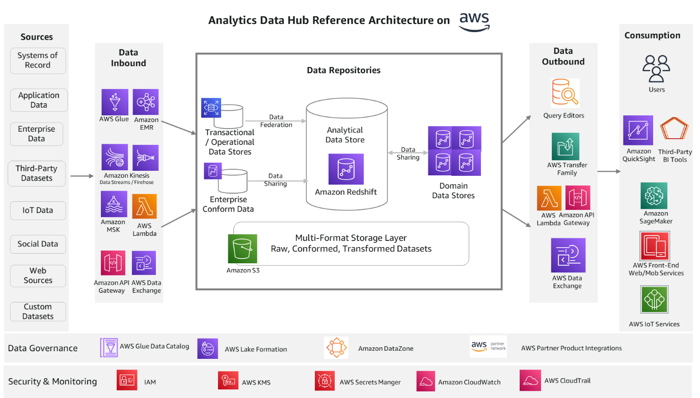
Let’s look at each component again and the relevant AWS services.
Data inbound services
AWS Glue and Amazon EMR services are ideal for batch processing. They scale automatically and are able to process most of the industry standard data formats. Amazon Kinesis Data Streams, Amazon Kinesis Data Firehose, and Amazon Managed Streaming for Apache Kafka (Amazon MSK) enables you to build streaming process applications. These streaming services integrate well with the Amazon Redshift streaming feature. This helps you process real-time sources, IoT data, and data from online channels. You can also ingest data with third-party tools like Informatica, dbt, and Matallion.
You can build RESTful APIs and WebSocket APIs using Amazon API Gateway and AWS Lambda, which will enable real-time two-way communication with web sources, social, and IoT sources. AWS Data Exchange helps with subscribing to third-party data in AWS Marketplace. Data subscription and access is fully managed with this service. Refer to the respective service documentation for further details.
Data repository services
Amazon Redshift is the recommended data storage service for OLAP (Online Analytical Processing) workloads such as cloud data warehouses, data marts, and other analytical data stores. This service is the core of this reference architecture on AWS and can address most analytical needs out of the box. You can use simple SQL to analyze structured and semi-structured data across data warehouses, data marts, operational databases, and data lakes to deliver the best price performance at any scale. The Amazon Redshift data sharing feature provides instant, granular, and high-performance access without data copies and data movement across multiple Amazon Redshift data warehouses in the same or different AWS accounts, and across Regions.
For ease of use, Amazon Redshift offers a serverless option. Amazon Redshift Serverless automatically provisions and intelligently scales data warehouse capacity to deliver fast performance for even the most demanding and unpredictable workloads, and you pay only for what you use. Just load your data and start querying right away in Amazon Redshift Query Editor or in your favorite BI tool and continue to enjoy the best price performance and familiar SQL features in an easy-to-use, zero administration environment.
Amazon Relational Database Service (Amazon RDS) is a fully managed service for building transactional and operational data stores. You can choose from many popular engines such as MySQL, PostgreSQL, MariaDB, Oracle, and SQL Server. With the Amazon Redshift federated query feature, you can query transactional and operational data in place without moving the data. The federated query feature currently supports Amazon RDS for PostgreSQL, Amazon Aurora PostgreSQL-Compatible Edition, Amazon RDS for MySQL, and Amazon Aurora MySQL-Compatible Edition.
Amazon Simple Storage Service (Amazon S3) is the recommended service for multi-format storage layers in the architecture. It offers industry-leading scalability, data availability, security, and performance. Organizations typically store data in Amazon S3 using open file formats. Open file formats enable analysis of the same Amazon S3 data using multiple processing and consumption layer components. Data in Amazon S3 can be easily queried in place using SQL with Amazon Redshift Spectrum. It helps you query and retrieve structured and semi-structured data from files in Amazon S3 without having to load the data. Multiple Amazon Redshift data warehouses can concurrently query the same datasets in Amazon S3 without the need to make copies of the data for each data warehouse.
Data outbound services
Amazon Redshift comes with the web-based analytics workbench Query Editor V2.0, which helps you run queries, explore data, create SQL notebooks, and collaborate on data with your teams in SQL through a common interface. AWS Transfer Family helps securely transfer files using SFTP, FTPS, FTP, and AS2 protocols. It supports thousands of concurrent users and is a fully managed, low-code service. Similar to inbound processes, you can utilize Amazon API Gateway and AWS Lambda for data pull using the Amazon Redshift Data API. And AWS Data Exchange helps publish your data to third parties for consumption through AWS Marketplace.
Consumption services
Amazon QuickSight is the recommended service for creating reports and dashboards. It enables you to create interactive dashboards, visualizations, and advanced analytics with ML insights. Amazon SageMaker is the ML platform for all your data science workload needs. It helps you build, train, and deploy models consuming the data from repositories in the data hub. You can use Amazon front-end web and mobile services and AWS IoT services to build web, mobile, and IoT endpoint applications to consume data out of the data hub.
Data governance services
The AWS Glue Data Catalog and AWS Lake Formation are the core data governance services AWS currently offers. These services help manage metadata centrally for all the data repositories and manage access controls. They also help with data classification and can automatically handle schema changes. You can use Amazon DataZone to discover and share data at scale across organizational boundaries with built-in governance and access controls. AWS is investing in this space to provide more a unified experience for AWS services. There are many partner products such as Collibra, Alation, Amorphic, Informatica, and more, which you can use as well for data governance functions with AWS services.
Security and monitoring services
AWS Identity and Access Management (AWS IAM) manages identities for AWS services and resources. You can define users, groups, roles, and policies for fine-grained access management of your workforce and workloads. AWS Key Management Service (AWS KMS) manages AWS keys or customer managed keys for your applications. Amazon CloudWatch and AWS CloudTrail help provide monitoring and auditing capabilities. You can collect metrics and events and analyze them for operational efficiency.
In this post, we’ve discussed the most common AWS services for the respective solution components. However, you aren’t limited to only these services. There are many other AWS services for specific use cases that may be more appropriate for your needs than what we discussed here. You can reach to AWS Analytics Solutions Architects for appropriate guidance.
Example architectures for gaming use cases
In this section, we discuss example architectures for two gaming use cases.
Game event analysis
In-game events (also called timed or live events) encourage player engagement through excitement and anticipation. Events entice players to interact with the game, increasing player satisfaction and revenue with in-game purchases. Events have become more and more important, especially as games shift from being static pieces of entertainment to be played as is to offering dynamic and changing content through the use of services that use information to make decisions about game play as the game is being played. This enables games to change as the players play and influence what works and what doesn’t, and gives any game a potentially infinite lifespan.
This capability of in-game events to offer fresh content and activities within a familiar framework is how you keep players engaged and playing for months to years. Players can enjoy new experiences and challenges within the familiar framework or world that they have grown to love.
The following example shows how such an architecture might appear, including changes to support various sections of the process like breaking the data into separate containers to accommodate scalability, charge-back, and ownership.
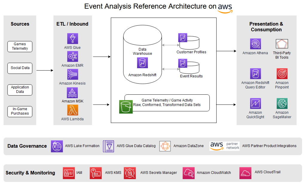
To fully understand how events are viewed by the players and to make decisions about future events requires information on how the latest event was actually performed. This means gathering a lot of data as the players play to build key performance indicators (KPIs) that measure the effectiveness and player satisfaction with each event. This requires analytics that specifically measure each event and capture, analyze, report on, and measure player experience for each event. These KPIs include the following:
- Initial user flow interactions – What actions users are taking after they first receive or download an event update in a game. Are there any clear drop-off points or bottlenecks that are turning people off the event?
- Monetization – When, what, and where users are spending money on in the event, whether it’s buying in-game currencies, answering ads, specials, and so on.
- Game economy – How can users earn and spend virtual currencies or goods during an event, using in-game money, trades, or barter.
- In-game activity – Player wins, losses, leveling up, competition wins, or player achievements within the event.
- User to user interactions – Invitations, gifting, chats (private and group), challenges, and so on during an event.
These are just some of the KPIs and metrics that are key for predictive modeling of events as the game acquires new players while keeping existing users involved, engaged, and playing.
In-game activity analysis
In-game activity analysis essentially looks at any meaningful, purposeful activity the player might show, with the goal of trying to understand what actions are taken, their timing, and outcomes. This includes situational information about the players, including where they are playing (both geographical and cultural), how often, how long, what they undertake on each login, and other activities.
The following example shows how such an architecture might appear, including changes to support various sections of the process like breaking the data into separate warehouses. The multi-cluster warehouse approach helps scale the workload independently, provides flexibility to the implemented charge-back model, and supports decentralized data ownership.
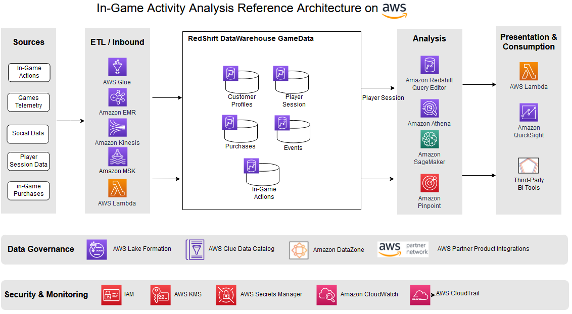
The solution essentially logs information to help understand the behavior of your players, which can lead to insights that increase retention of existing players, and acquisition of new ones. This can provide the ability to do the following:
- Provide in-game purchase recommendations
- Measure player trends in the short term and over time
- Plan events the players will engage in
- Understand what parts of your game are most successful and which are less so
You can use this understanding to make decisions about future game updates, make in-game purchase recommendations, determine when and how your game economy may need to be balanced, and even allow players to change their character or play as the game progresses by injecting this information and accompanying decisions back into the game.
Conclusion
This reference architecture, while showing examples of only a few analysis types, provides a faster technology path for enabling game analytics applications. The decoupled, hub/spoke approach brings the agility and flexibility to implement different approaches to analytics and understanding the performance of game applications. The purpose-built AWS services described in this architecture provide comprehensive capabilities to easily collect, store, measure, analyze, and report game and event metrics. This helps you efficiently perform in-game analytics, event analysis, measure player satisfaction, and provide tailor-made recommendations to game players, efficiently organize events, and increase retention rates.
Thanks for reading the post. If you have any feedback or questions, please leave them in the comments.
About the authors
 Satesh Sonti is a Sr. Analytics Specialist Solutions Architect based out of Atlanta, specialized in building enterprise data platforms, data warehousing, and analytics solutions. He has over 16 years of experience in building data assets and leading complex data platform programs for banking and insurance clients across the globe.
 Tanya Rhodes is a Senior Solutions Architect based out of San Francisco, focused on games customers with emphasis on analytics, scaling, and performance enhancement of games and supporting systems. She has over 25 years of experience in enterprise and solutions architecture specializing in very large business organizations across multiple lines of business including games, banking, healthcare, higher education, and state governments.
Amazon Athena is a serverless, interactive analytics service built on open-source frameworks, supporting open-table and file formats. Athena provides a simplified, flexible way to analyze petabytes of data where it lives. You can analyze data or build applications from an Amazon Simple Storage Service (Amazon S3) data lake and over 25 data sources, including on-premises data sources or other cloud systems using SQL or Python. Athena is built on open-source Trino and Presto engines and Apache Spark frameworks, with no provisioning or configuration effort required.
Different types of users rely on Athena, including business analysts, data scientists, security, and operations engineers. Athena provides a query editor to enter and run queries on data using structured query language (SQL). The query editor provides features like run, cancel, and save queries or statements. Additionally, it provides keyboard shortcuts for user-friendly operation.
This post discusses the keyboard shortcuts available and how you can use them.
Accessing the Athena console
If you’re new to Athena and don’t know how to access the Athena console and run queries and statements, refer to the following getting started tutorial. This tutorial walks you through using Athena to query data. You’ll create a table based on sample data stored in Amazon S3, query the table, and check the results of the query.
Keyboard shortcuts
The query editor provides keyboard shortcuts for different action types like running a query, formatting a query, line operations, selection, multi-cursor, go to, find/replace, and folding. Compared to reaching for the mouse or navigating a menu, a single keyboard shortcut saves a moment of your time.
With keyboard shortcuts, you can use key combinations to edit your SQL statement without using a mouse. For example, you can use multiple cursors in your editing window for selecting all instances of text you wish to edit, and edit your text, fold or unfold selected text, find and replace text, and perform line operations like remove line, move lines, and more.
You can also find these keyboard shortcuts on the query editor on the bottom right corner, as highlighted in the following screenshot.

The following table shows the keyboards shortcuts for Window/Linux and Mac.
| Action Type | Action | Windows/Linux | Mac |
| Other | Execute query | Ctrl-Enter | Cmd-Enter, Ctrl-Enter |
| Other | Format query | Ctrl-Alt-L | Opt-Cmd-L |
| Other | Previous query | Ctrl-Up | Ctrl-Shift-Up |
| Other | Next query | Ctrl-Down | Ctrl-Shift-Down |
| Other | Close tab | Alt-X | Opt-X |
| Other | Previous tab | Ctrl-, | Ctrl-, |
| Other | Next tab | Ctrl-. | Ctrl-. |
| Other | Indent | Tab | Tab |
| Other | Outdent | Shift-Tab | Shift-Tab |
| Other | Save | Ctrl-S | Cmd-S |
| Other | Undo | Ctrl-Z | Cmd-Z |
| Other | Redo | Ctrl-Shift-Z, Ctrl-Y | Cmd-Shift-Z, Cmd-Y |
| Other | Toggle comment | Ctrl-/ | Cmd-/ |
| Other | Transpose letters | Ctrl-T | Ctrl-T |
| Other | Change to lower case | Ctrl-Shift-U | Ctrl-Shift-U |
| Other | Change to upper case | Ctrl-U | Ctrl-U |
| Other | Overwrite | Insert | Insert |
| Other | Delete | Delete | – |
| Line Operations | Remove line | Ctrl-D | Cmd-D |
| Line Operations | Copy lines down | Alt-Shift-Down | Cmd-Opt-Down |
| Line Operations | Copy lines up | Alt-Shift-Up | Cmd-Opt-Up |
| Line Operations | Move lines down | Alt-Down | Opt-Down |
| Line Operations | Move lines up | Alt-Up | Opt-Up |
| Line Operations | Remove to line end | Alt-Delete | Ctrl-K |
| Line Operations | Remove to line start | Alt-Backspace | Cmd-Backspace |
| Line Operations | Remove word left | Ctrl-Backspace | Opt-Backspace, Ctrl-Opt-Backspace |
| Line Operations | Remove word right | Ctrl-Delete | Opt-Delete |
| Line Operations | Split line | – | Ctrl-O |
| Selection | Select all | Ctrl-A | Cmd-A |
| Selection | Select left | Shift-Left | Shift-Left |
| Selection | Select right | Shift-Right | Shift-Right |
| Selection | Select word left | Ctrl-Shift-Left | Opt-Shift-Left |
| Selection | Select word right | Ctrl-Shift-Right | Opt-Shift-Right |
| Selection | Select line start | Shift-Home | Shift-Home |
| Selection | Select line end | Shift-End | Shift-End |
| Selection | Select to line end | Alt-Shift-Right | Cmd-Shift-Right |
| Selection | Select to line start | Alt-Shift-Left | Cmd-Shift-Left |
| Selection | Select up | Shift-Up | Shift-Up |
| Selection | Select down | Shift-Down | Shift-Down |
| Selection | Select page up | Shift-PageUp | Shift-PageUp |
| Selection | Select page down | Shift-PageDown | Shift-PageDown |
| Selection | Select to start | Ctrl-Shift-Home | Cmd-Shift-Up |
| Selection | Select to end | Ctrl-Shift-End | Cmd-Shift-Down |
| Selection | Duplicate selection | Ctrl-Shift-D | Cmd-Shift-D |
| Selection | Select to matching bracket | Ctrl-Shift-P | – |
| Multicursor | Add multi-cursor above | Ctrl-Alt-Up | Ctrl-Opt-Up |
| Multicursor | Add multi-cursor below | Ctrl-Alt-Down | Ctrl-Opt-Down |
| Multicursor | Add next occurrence to multi-selection | Ctrl-Alt-Right | Ctrl-Opt-Right |
| Multicursor | Add previous occurrence to multi-selection | Ctrl-Alt-Left | Ctrl-Opt-Left |
| Multicursor | Move multi-cursor from current line to the line above | Ctrl-Alt-Shift-Up | Ctrl-Opt-Shift-Up |
| Multicursor | Move multi-cursor from current line to the line below | Ctrl-Alt-Shift-Down | Ctrl-Opt-Shift-Down |
| Multicursor | Remove current occurrence from multi-selection and move to next | Ctrl-Alt-Shift-Right | Ctrl-Opt-Shift-Right |
| Multicursor | Remove current occurrence from multi-selection and move to previous | Ctrl-Alt-Shift-Left | Ctrl-Opt-Shift-Left |
| Multicursor | Select all from multi-selection | Ctrl-Shift-L | Ctrl-Shift-L |
| Go to | Go to left | Left | Left, Ctrl-B |
| Go to | Go to right | Right | Right, Ctrl-F |
| Go to | Go to word left | Ctrl-Left | Opt-Left |
| Go to | Go to word right | Ctrl-Right | Opt-Right |
| Go to | Go line up | Up | Up, Ctrl-P |
| Go to | Go line down | Down | Down, Ctrl-N |
| Go to | Go to line start | Alt-Left, Home | Cmd-Left, Home, Ctrl-A |
| Go to | Go to line end | Alt-Right, End | Cmd-Right, End, Ctrl-E |
| Go to | Go to page up | PageUp | Opt-PageUp |
| Go to | Go to page down | PageDown | Opt-PageDown, Ctrl-V |
| Go to | Go to start | Ctrl-Home | Cmd-Home, Cmd-Up |
| Go to | Go to end | Ctrl-End | Cmd-End, Cmd-Down |
| Go to | Scroll line down | Ctrl-Down | Cmd-Down |
| Go to | Scroll line up | Ctrl-Up | – |
| Go to | Go to matching bracket | Ctrl-P | – |
| Go to | Scroll page down | – | Opt-PageDown |
| Go to | Scroll page up | – | Opt-PageUp |
| Find/Replace | Find | Ctrl-F | Cmd-F |
| Find/Replace | Replace | Ctrl-H | Cmd-Opt-F |
| Find/Replace | Find next | Ctrl-K | Cmd-G |
| Find/Replace | Find previous | Ctrl-Shift-K | Cmd-Shift-G |
| Folding | Fold selection | Alt-L, Ctrl-F1 | Cmd-Opt-L, Cmd-F1 |
| Folding | Unfold | Alt-Shift-L, Ctrl-Shift-F1 | Cmd-Opt-Shift-L, Cmd-Shift-F1 |
| Folding | Unfold all | Alt-Shift-0 | Cmd-Opt-Shift-0 |
| Other | Autocomplete | Ctrl-Space | Ctrl-Space |
| Other | Focus out | Esc | Esc |
For illustration, you can perform the Format query action by using the keyboard shortcut (Ctrl-Alt-L for Windows/Linux, Opt-Cmd-L for Mac). It converts unformatted SQL to a well-formatted SQL, as shown in the following screenshots.

Similarly, you can try out the Toggle comment command (Ctrl-/ for Windows/Linux, Cmd-/ for Mac) to comment or uncomment lines of SQL in the Athena query editor. This comes in very handy when you want to quickly comment out specific lines in your query, as shown in the following screenshots.

You can do line operations like Remove line, Copy lines down, Copy lines up, and more. The following screenshots show an example of the Remove line action (Ctrl-D for Windows/Linux, Cmd-D for Mac).

You can do a line selection like Select all, Select left, Select line start, and more. The following screenshots show an example the Select all action (Ctrl-A for Windows/Linux, Cmd-A for Mac).

You can do multi-cursor actions like Add multi-cursor above, Add multi-cursor below, Add next occurrence to multi-selection, Add previous occurrence to multi-selection, Move multi-cursor from current line to the line above, and more. The following example is of the Add multi-cursor above action (Ctrl-Alt-Up for Windows/Linux, Ctrl-Opt-Up for Mac).

You can do go to actions like Go to left, Go to right, Go to word left, and more. The following is an example of the Go to left action (Ctrl-B).

You can do find and replace actions like Find, Replace, Find next, and more. The following is an example of the Replace action (Ctrl-H for Windows/Linux, Cmd-Opt-F for Mac).

You can also do folding actions like Fold selection, Unfold, and Unfold all. The following example is of the Unfold action (Alt-Shift-L or Ctrl-Shift-F1 for Windows/Linux, Cmd-Opt-Shift-L or Cmd-Shift-F1 for Mac).

Conclusion
In this post, we saw how Athena provides an array of native options to help you improve productivity when analyzing your data. You can go to the Athena console and start running SQL statements or querying data using the built-in query editor. The query editor provides key shortcuts to improve your productivity by using key combinations to edit SQL statements, instead of using a mouse.
If you have any questions or suggestions, please leave a comment.
About the Authors
 Naresh Gautam is a Data Analytics and AI/ML leader at AWS with 20 years of experience, who enjoys helping customers architect highly available, high-performance, and cost-effective data analytics and AI/ML solutions to empower customers with data-driven decision-making. In his free time, he enjoys meditation and cooking.
 Srikanth Sopirala is a Principal Analytics Specialist Solutions Architect at AWS. He is a seasoned leader with over 20 years of experience, who is passionate about helping customers build scalable data and analytics solutions to gain timely insights and make critical business decisions. In his spare time, he enjoys reading, spending time with his family, and road biking.
 Harsh Vardhan is an AWS Solutions Architect, specializing in analytics. He has over 5 years of experience working in the field of big data and data science. He is passionate about helping customers adopt best practices and discover insights from their data.
Building data lakes from continuously changing transactional data of databases and keeping data lakes up to date is a complex task and can be an operational challenge. A solution to this problem is to use AWS Database Migration Service (AWS DMS) for migrating historical and real-time transactional data into the data lake. You can then apply transformations and store data in Delta format for managing inserts, updates, and deletes.
Amazon EMR Serverless is a serverless option in Amazon EMR that makes it easy for data analysts and engineers to run open-source big data analytics frameworks without configuring, managing, and scaling clusters or servers. EMR Serverless automatically provisions and scales the compute and memory resources required by your applications, and you only pay for the resources that the applications use. EMR Serverless also provides you with more flexibility on overriding default Spark configurations, customizing EMR Serverless images, and customizing Spark driver and executor sizes to better suit specific workloads.
This post demonstrates how to implement a solution that uses AWS DMS to stream ongoing replication or change data capture (CDC) from an Amazon Aurora PostgreSQL-Compatible Edition database into Amazon Simple Storage Service (Amazon S3). We then apply transformations using Spark jobs on an EMR Serverless application and write transformed output into open-source Delta tables in Amazon S3. The Delta tables created by the EMR Serverless application are exposed through the AWS Glue Data Catalog and can be queried through Amazon Athena. Although this post uses an Aurora PostgreSQL database hosted on AWS as the data source, the solution can be extended to ingest data from any of the AWS DMS supported databases hosted on your data centers.
Solution overview
The following diagram shows the overall architecture of the solution that we implement in this post.

The solution consists of the following steps for implementing a full and incremental (CDC) data ingestion from a relational database:
- Data storage and data generation – We create an Aurora PostgreSQL database and generate fictional trip data by running a stored procedure. The data will have attributes like trip ID (primary key), timestamp, source location, and destination location. Incremental data is generated in the PostgreSQL table by running custom SQL scripts.
- Data ingestion – Steps 1 and 2 use AWS DMS, which connects to the source database and moves full and incremental data (CDC) to Amazon S3 in Parquet format. Let’s refer to this S3 bucket as the raw layer.
- Data transformation – Steps 3 and 4 represent an EMR Serverless Spark application (Amazon EMR 6.9 with Apache Spark version 3.3.0) created using Amazon EMR Studio. The script reads input data from the S3 raw bucket, and then invokes Delta Lake’s MERGE statements to merge the data with the target S3 bucket (curated layer). The script also creates and updates a manifest file on Amazon S3 every time the job is run to enable data access from Athena and Amazon Redshift Spectrum.
- Data access – The EMR Serverless job has code snippets that create a Delta table in the AWS Glue Data Catalog in Step 5. Steps 6 and 7 describe using Athena and Redshift Spectrum to query data from the Delta tables using standard SQL through the AWS Glue Data Catalog.
- Data pipeline – Step 8 describes the process for triggering the data pipeline in a periodic manner through Airflow operators using Amazon Managed Workflows for Apache Airflow (Amazon MWAA). Refer to Submitting EMR Serverless jobs from Airflow for additional details. In this post, AWS DMS has been configured to replicate data from Amazon Aurora PostgreSQL-Compatible Edition into an S3 bucket with hourly partitions. The Airflow DAG can be configured to call an EMR Serverless job to process the past X hours of data based on specific project requirements. Implementation of the Airflow setup is not explored within the scope of this post.
The architecture has the following major features:
- Reliability – The end-to-end architecture is made resilient with the Multi-AZ feature of EMR Serverless and using Multi-AZ deployments for AWS DMS and Amazon Aurora PostgreSQL-Compatible Edition. When you submit jobs to an EMR Serverless application, those jobs are automatically distributed to different Availability Zones in the Region. A job is run in a single Availability Zone to avoid performance implications of network traffic across Availability Zones. In case an Availability Zone is impaired, a job submitted to your EMR Serverless application is automatically run in a different (healthy) Availability Zone. When using resources in a private VPC, EMR Serverless recommends that you specify the private VPC configuration for multiple Availability Zones so that EMR Serverless can automatically select a healthy Availability Zone.
- Cost optimization – When you run Spark or Hive applications using EMR Serverless, you pay for the amount of vCPU, memory, and storage resources consumed by your applications, leading to optimal utilization of resources. There is no separate charge for Amazon Elastic Compute Cloud (Amazon EC2) instances or Amazon Elastic Block Store (Amazon EBS) volumes. For additional details on cost, refer to Amazon EMR Serverless cost estimator.
- Performance efficiency – You can run analytics workloads at any scale with automatic on-demand scaling that resizes resources in seconds to meet changing data volumes and processing requirements. EMR Serverless includes the Amazon EMR performance-optimized runtime for Apache Spark and Hive. The Amazon EMR runtime for Spark is 100% API-compatible with OSS Spark and is over 3.5 times as fast as the standard open-source, so your jobs run faster and incur less compute costs. With fast and fine-grained scaling in EMR Serverless, if a pipeline runs daily and needs to process 1 GB of data one day and 100 GB of data another day, EMR Serverless automatically scales to handle that load.
- Monitoring – EMR Serverless sends metrics to Amazon CloudWatch at the application and job level every 1 minute. You can set up a single-view dashboard in CloudWatch to visualize application-level and job-level metrics using an AWS CloudFormation template provided on the EMR Serverless CloudWatch Dashboard GitHub repository. Also, EMR Serverless can store application logs in a managed storage, Amazon S3, or both based on your configuration settings. After you submit a job to an EMR Serverless application, you can view the real-time Spark UI or the Hive Tez UI for the running job from the EMR Studio console or request a secure URL using the GetDashboardForJobRun API. For completed jobs, you can view the Spark History Server or the Persistent Hive Tez UI from the EMR Studio console.
The following steps are performed to implement this solution:
- Connect to the Aurora PostgreSQL instance and generate a sample dataset.
- Set up a data pipeline for loading data from Amazon Aurora PostgreSQL-Compatible Edition into Delta Lake on Amazon S3 and query using Athena:
- Start the AWS DMS task to perform full table load and capture ongoing replication to the S3 raw layer.
- Run the EMR Serverless Spark application to load data into Delta Lake.
- Query the Delta tables (native tables) through Athena.
- Run the data pipeline to capture incremental data changes into Delta Lake:
- Generate an incremental (CDC) dataset and insert it into the Aurora PostgreSQL database.
- Run the EMR Serverless Spark application to merge CDC data in the S3 curated layer (incremental load).
- Query the Delta Lake tables through Athena to validate the merged data.
Prerequisites
We use a CloudFormation template to provision the AWS resources required for the solution. The CloudFormation template requires you to select an EC2 key pair. This key is configured on an EC2 instance that lives in the public subnet. We use this EC2 instance to connect to the Aurora PostgreSQL instance that lives in the private subnet. Make sure you have a key in the Region where you deploy the template. If you don’t have one, you can create a new key pair.
To walk through this post, we use Delta Lake version > 2.0.0, which is supported in Apache Spark 3.2.x. Choose the Delta Lake version compatible with your Spark version by visiting the Delta Lake releases page. We use an EMR Serverless application with version emr-6.9.0, which supports Spark version 3.3.0.
Deploy your resources
To provision the resources needed for the solution, complete the following steps:
- Choose Launch Stack:
- For Stack name, enter
emr-serverless-deltalake-blog. - For DatabaseUserName, enter the user name for logging in to Amazon Aurora PostgreSQL-Compatible Edition. Keep the default value if you don’t want to change it.
- For DatabasePassword, enter the password for logging in to Amazon Aurora PostgreSQL-Compatible Edition.
- For ClientIPCIDR, enter the IP address of your SQL client that will be used to connect to the EC2 instance. We use this EC2 instance to connect to the Aurora PostgreSQL database.
- For KeyName, enter the key pair to be used in your EC2 instance. This EC2 instance will be used as a proxy to connect from your SQL client to the Aurora PostgreSQL source database.
- For EC2ImageId, PrivateSubnet1CIDR, PrivateSubnet2CIDR, PublicSubnetCIDR, and VpcCIDR, keep the default values or choose appropriate values for the VPC and EC2 image for your specific environment.
- Choose Next.
- Choose Next again.
- On the review page, select I acknowledge that AWS CloudFormation might create IAM resources with custom names.
- Choose Create stack.
After the CloudFormation template is complete and the resources are created, the Outputs tab shows the information shown in the following screenshot.

The CloudFormation template creates all the resources needed for the solution workflow:
- S3 raw and curated buckets
- Aurora PostgreSQL database
- AWS DMS migration task, replication instance, and other resources
- EC2 instance for running data ingestion scripts
- AWS Identity and Access Management (IAM) roles and policies needed to perform the necessary activities as part of this solution
- VPC, subnets, security groups, and relevant network components
- AWS Lambda functions that perform setup activities required for this workflow
- Additional components needed for running the EMR Serverless workflow
You can find the PySpark script in the raw S3 bucket on the Amazon S3 console as shown in the following screenshot. The bucket will have the naming structure <CloudFormation template name>-rawS3bucket-<random string>. Make a note of the S3 path to the emr\_delta\_cdc.py script; you need this information while submitting the Spark job via the EMR Serverless application.

The preceding task for creating the resources via CloudFormation assumes that AWS Lake Formation is not enabled in the Region (which we enable later in this post). If you already have Lake Formation enabled in the Region, make sure the IAM user or role used in the CloudFormation template has the necessary permissions to create a database in the AWS Glue Data Catalog.
Connect to the Aurora PostgreSQL instance and generate a sample dataset
Connect to the Aurora PostgreSQL endpoint using your preferred client. For this post, we use the PSQL command line tool. Note that the IP address of the client machine from which you’re connecting to the database must be updated in the Aurora PostgreSQL security group. This is done by the CloudFormation template based on the input parameter value for ClientIPCIDR. If you’re accessing the database from another machine, update the security group accordingly.
- Connect to your EC2 instance from the command line using the public DNS of the EC2 instance from the CloudFormation template output.
- Log in to the EC2 instance and connect to the Aurora PostgreSQL instance using the following commands (the Aurora PostgreSQL endpoint is available on the Outputs tab of the CloudFormation stack):

- Run the following commands to create a schema and table for the fictional trip dataset:

- Create the following stored procedure to generate the records for the trip dataset and insert the records into the table.
- Call the preceding stored procedure to insert 20,000 records into the Aurora PostgreSQL database:
- After the stored procedure is complete, verify that the records have been inserted successfully:

Set up a data pipeline for loading data into Delta tables on Amazon S3 and query using Athena
In this section, we walk through the steps to set up a data pipeline that loads data from Amazon Aurora PostgreSQL-Compatible Edition into Delta tables on Amazon S3 and then query the data using Athena.
Start the AWS DMS task to perform full table load to the S3 raw layer
To perform the full table load, complete the following steps:
- On the AWS DMS console, choose Database migration tasks in the navigation pane.
- Select the task that was created by the CloudFormation template (
emrdelta-postgres-s3-migration). - On the Actions menu, choose Restart/Resume.
The task starts the full load and ongoing replication of data from the source database to Amazon S3.

- Wait for the job to complete.
You can validate that the data has been migrated successfully checking the Load state column for the AWS DMS task.

- Navigate to the S3 bucket created from the CloudFormation template to store raw data from AWS DMS.The bucket will have the naming structure
<CloudFormation template name>-rawS3bucket-<random string>. - Navigate to the folder
delta\_emr\_source/travel\_detailsin the raw S3 bucket. You can verify the S3 folder has Parquet data populated from the AWS DMS task.
Run the EMR Serverless Spark application to load data into Delta tables
We use EMR Studio to manage and submit jobs in an EMR Serverless application.
- Launch EMR Studio and create an EMR Serverless application.
- For Name, enter
emr-delta-blog. - For Type, choose Spark.
- For Release version, choose your release version.
- For Architecture, select x86\_64.
- For Application setup options, select Choose default settings.

- Choose Create application and verify that the EMR application has been created successfully on the Amazon EMR console.

- Choose
emr\_delta\_blogand then choose Start application. You can verify that the EMR application has started successfully on the Amazon EMR console, as shown in the following screenshot.

The application will move to Stopped status after a period of inactivity. When you submit the job to the application, it will start again and start the job. This provides cost savings because the jobs are run on demand as opposed to maintaining a running EMR cluster.
- While the application is in Started status, choose Submit job to submit the job to the application.
 Create a new job in the Job details page
- For Name, enter
emr-delta-load-job. - For Runtime role, choose
emrserverless-execution-role. - For S3 URI, enter the S3 (raw bucket) path where the script
emr\_delta\_cdc.pyis uploaded. - For Script arguments, enter
["I","delta\_emr\_source","9999-12-31-01","travel\_details","route\_id"].
 The script arguments provide the following details to the EMR Serverless application:
- I – The first argument represents the data load type. The allowed values are I for full load and U for incremental data load.
- delta\_emr\_source – The second argument represents the source database schema from which data is being migrated through the AWS DMS task.
- 9999-12-31-01 – The third argument represents the partition from which data needs to be loaded in an incremental fashion. This argument is used only during CDC data load; for full load, we have provided a default value (9999-12-31-01).
- travel\_details – The fourth argument represents the source database table from which data is being migrated through the AWS DMS task. Use a semicolon as a delimiter when entering multiple tables.
- route\_id – The fifth argument represents the partition keys on which the table data should be partitioned when stored in the S3 curated bucket. Use a semicolon as a delimiter when entering comma-separated partition keys for multiple tables.
With arguments, you can group a set of tables and submit the job to an EMR Serverless application. You can provide multiple table names separated by semicolons and enter the partition keys for those tables also separated by semicolon. If a particular table doesn’t have a partition key, simply enter a semicolon alone. The number of semicolon-separated values should match the table and partition key arguments for the script to run successfully.
Also, if you want to capture additional tables as part of an existing EMR Serverless job, you need to create a new EMR Serverless job to capture full load separately (set the first argument as I along with the new table names) and then change the argument list of the existing EMR Serverless job to add those new tables to capture incremental data load going forward.
EMR Serverless version 6.9.0 comes pre-installed with Delta version 2.1.0. Refer to About Amazon EMR Releases for more details about pre-installed libraries and applications for a specific Amazon EMR release. Before this, we have to upload the Delta JAR files to an S3 bucket in your account and provide the JAR file path in the application configurations using the spark.jars option. In this walkthrough, we create an EMR Serverless 6.9.0 application and use the pre-installed Delta jars from Amazon EMR.
- Under Spark properties, choose Edit in text and enter the following configurations:
If you want to use a different version of Delta JAR files, you can replace the S3 path of the JAR files in these configuration options.
- Leave the rest of the configurations at their default and choose Submit job.
- Wait for the job to complete successfully. You can verify this on the EMR Serverless console.

- Additionally, go to the S3 location (the curated bucket created by AWS CloudFormation) and verify that the Delta files are created along with the manifest file.

- Select a job run and then choose Spark History Server (Completed jobs) on the View Application UIs menu.

You can now use the Spark History Server UI to navigate to various tabs and analyze the job run in a detailed manner. For Spark error and output logs, you can navigate to the Executors tab and explore the driver or executor logs as required. This can help you to debug the job in case of failures by looking at the Spark logs.You can also choose Spark UI (Running jobs) to track the progress of the EMR Serverless Spark jobs while they are running.

The data load script is the same for initial and incremental data load because it can handle both the workflows through script arguments:
Monitor EMR Serverless application using CloudWatch dashboards
We can optionally monitor the EMR Serverless application using CloudWatch dashboards by installing the CloudFormation template from the EMR Serverless CloudWatch Dashboard GitHub repository.Follow the instructions on the Getting started section on the GitHub repository and deploy the CloudFormation template in your account.
You need to provide the EMR Serverless application ID as a parameter while deploying the CloudFormation stack, which can be obtained on the EMR Studio Applications page as shown in the following screenshot.

After the CloudFormation template is successfully deployed, navigate to the CloudWatch console to see a custom dashboard created for the EMR Serverless application ID that was provided to the CloudFormation template.

Choose the dashboard to see the different metrics for the EMR Serverless application in a single dashboard view.
You can see the available workers (one driver and two executors that were pre-initialized in the default configuration) and also the spike under successful job count that indicates the initial data load job that was completed successfully.

You could also monitor the CPU, memory, and storage allocated for the application, driver, and executor nodes separately.
The following image shows application metrics for three workers with 12 vCPUs (both driver and executor initialized with 4 vCPUs) and also the memory and storage usage. You can monitor the metrics from this dashboard and pre-initialize your application capacity that suits your specific workloads.

We can see the number of executors that were utilized for this job execution from the executor metrics section within the CloudWatch dashboard. We have used two executors and a driver for running this job.

Query the Delta tables through Athena
Previously, Delta tables were accessed through Athena by generating the manifest files (which maintain the list of data files to read for querying a Delta table). With the newly launched support in Athena for reading native Delta tables, it’s no longer required to generate and update manifest files. The Athena SQL engine version 3 can directly query native Delta tables. If you’re using an older engine version, change the engine version.
Navigate to the Athena console and start querying the data. Run a SELECT query and fetch the first 10 records to verify the data:

The table (native Delta table) has been created and updated to the AWS Glue Data Catalog from the EMR Serverless application code. You can successfully query and explore the data through Athena or Spark applications, but the schema definitions for individual columns aren’t updated in Data Catalog with this approach.
The following screenshot shows the Delta table created through code has a single array column. Athena supports reading native Delta tables and therefore we can read the data successfully even though the Data Catalog shows only a single array column.

If you need the individual column-level metadata to be available in the Data Catalog, run an AWS Glue crawler periodically to keep the AWS Glue metadata updated. For more information, refer to Introducing native Delta Lake table support with AWS Glue crawlers.
Run the data pipeline to load incremental data changes into the Delta tables
In this section, we walk through the steps to run the data pipeline.
Generate an incremental (CDC) dataset and insert it into the Aurora PostgreSQL database
- Log in to the EC2 instance via SSH and using the PSQL CLI, run the following SQL commands to generate CDC data on the source database:
update delta\_emr\_source.travel\_details set destination='Tucson' where destination='Miami';
call delta\_emr\_source.insert\_records(200);
delete from delta\_emr\_source.travel\_details where destination='Los Angeles';

- Navigate to the AWS DMS console and verify whether the incremental records are populated to the S3 raw bucket by the replication task.

You can also verify in the S3 raw bucket location that the files are created under hourly partitioned folders.

Run the EMR Serverless Spark application to merge CDC data in the S3 curated layer (incremental load)
After the AWS DMS task has successfully loaded the incremental data, submit the Spark job on the EMR Serverless application to load the incremental data (CDC) with the following script arguments:
The partition path given here as 2022-10-25-21 should be changed as applicable in your use case. We use an example use case where the EMR Serverless job runs every hour, and the input data folder is partitioned on an hourly basis from AWS DMS. You can choose an appropriate partitioning strategy on the S3 raw bucket for your use case.
- Under Spark properties, choose Edit in text and enter the following configurations:

- When the job is successful, verify in Amazon S3 that more files are created in the
\_delta\_logfolder, capturing the changes from the current run.
 Query the Delta tables through Athena to validate the merged data
Go to the Athena console to query the data and validate count to ensure that the table contains the most recent data:

If you also want to query this data from Amazon Redshift, you can create external tables in Redshift Spectrum for Delta tables. For more information, refer to Creating external tables for data managed in Delta Lake. Redshift Spectrum currently supports querying Delta tables through the manifest file option. A Delta table manifest contains a list of files that make up a consistent snapshot of the Delta table. The code snippet given in this post updates the manifest files every time new data is loaded in the Delta tables to ensure only the latest data is read from the Delta tables.
Clean up
To avoid incurring ongoing charges, clean up your infrastructure by deleting the stack from the AWS CloudFormation console. Delete the EMR Serverless application and any other resources you created during this exercise.
Conclusion
In this post, we demonstrated how to create a transactional data lake with Delta table format using EMR Serverless and AWS DMS. With the flexibility provided by EMR Serverless, you can use the latest version of open-source Delta framework on EMR Serverless (with the latest version of Spark) in order to support a wider range of transactional data lake needs based on various use cases.
Now you can build a transactional data lake for your organization with Delta table format and access data using Athena and Redshift Spectrum for various analytical workloads. You could use this high-level architecture for any other use cases where you need to use the latest version of Spark on EMR Serverless.
About the Authors
 Sankar Sundaram is a Data Lab Architect at AWS, where he helps customers build and modernize data architectures and help them build secure, scalable, and performant data lake, database, and data warehouse solutions.
 Monjumi Sarma is a Data Lab Solutions Architect at AWS. She helps customers architect data analytics solutions, which gives them an accelerated path towards modernization initiatives.
This is a guest post co-written with Parag Doshi, Guru Havanur, and Simon Guindon from Tricentis.
Tricentis is the global leader in continuous testing for DevOps, cloud, and enterprise applications. It has been well published since the State of DevOps 2019 DORA Metrics were published that with DevOps, companies can deploy software 208 times more often and 106 times faster, recover from incidents 2,604 times faster, and release 7 times fewer defects. Speed changes everything, and continuous testing across the entire CI/CD lifecycle is the key. However, speed is only realized when you have the confidence to release software on demand. Tricentis instills that confidence by providing software tools that enable Agile Continuous Testing (ACT) at scale. Whether exploratory or automated, functional or performance, API or UI, targeting mainframes, custom applications, packaged applications, or cloud-native applications, Tricentis provides a comprehensive suite of specialized continuous testing tools that help its customers achieve the confidence to release on demand.
The next phase of Tricentis’ journey is to unlock insights across all testing tools. Teams may struggle to have a unified view of software quality due to siloed testing across many disparate tools. For users that require a unified view of software quality, this is unacceptable. In this post, we share how the AWS Data Lab helped Tricentis to improve their software as a service (SaaS) Tricentis Analytics platform with insights powered by Amazon Redshift.
The challenge
Tricentis provides SaaS and on-premises solutions to thousands of customers globally. Every change to software worth testing is tracked in test management tools such as Tricentis qTest, test automation tools such as Tosca or Testim, or performance testing tools such as Neoload. Although Tricentis has amassed such data over a decade, the data remains untapped for valuable insights. Each of these tools has its own reporting capabilities that make it difficult to combine the data for integrated and actionable business insights.
Additionally, the scale is significant because the multi-tenant data sources provide a continuous stream of testing activity, and our users require quick data refreshes as well as historical context for up to a decade due to compliance and regulatory demands.
Finally, data integrity is of paramount importance. Every event in the data source can be relevant, and our customers don’t tolerate data loss, poor data quality, or discrepancies between the source and Tricentis Analytics. While aggregating, summarizing, and aligning to a common information model, all transformations must not affect the integrity of data from its source.
The solution
Tricentis Analytics aims to address the challenges of high volume, near-real-time, and visually appealing reporting and analytics across the entire Tricentis product portfolio.
The initial customer objectives were:
- Provide export of data securely accessible from the AWS Cloud
- Provide an initial set of pre-built dashboards that provide immediate business insights
- Beta test a solution with early adopter customers within 6 weeks
Considering the multi-tenant data source, Tricentis and the AWS Data Lab team engineered for the following constraints:
- Deliver the end-to-end pipeline to load only the eligible customers into an analytics repository
- Transform the multi-tenant data into single-tenant data isolated for each customer in strictly segregated environments
Knowing that data will be unified across many sources deployed in any environment, the architecture called for an enterprise-grade analytics platform. The data pipeline consists of multiple layers:
- Ingesting data from the source either as application events or change data capture (CDC) streams
- Queuing data so that we can rewind and replay the data back in time without going back to the source
- Light transformations such as splitting multi-tenant data into single tenant data to isolate customer data
- Persisting and presenting data in a scalable and reliable lake house (data lake and data warehouse) repository
Some customers will access the repository directly via an API with the proper guardrails for stability to combine their test data with other data sources in their enterprise, while other customers will use dashboards to gain insights on testing. Initially, Tricentis defines these dashboards and charts to enable insight on test runs, test traceability with requirements, and many other pre-defined use cases that can be valuable to customers. In the future, more capabilities will be provided to end-users to come up with their own analytics and insights.
How Tricentis and the AWS Data Lab were able to establish business insights in 6 weeks
Given the challenge of Tricentis Analytics with live customers in 6 weeks, Tricentis partnered with the AWS Data Lab. From detailed design to a beta release, Tricentis had customers expecting to consume data from a data lake specific to only their data, and all of the data that had been generated for over a decade. Customers also required their own repository, an Apache Parquet data lake, which would combine with other data in the customer environment to gather even greater insights.
The AWS account team proposed the AWS Data Lab Build Lab session to help Tricentis accelerate the process of designing and building their prototype. The Build Lab is a two-to-five-day intensive build by a team of customer builders with guidance from an AWS Data Lab Solutions Architect. During the Build Lab, the customer will construct a prototype in their environment, using their data, with guidance on real-world architectural patterns and anti-patterns, as well as strategies for building effective solutions, from AWS service experts. Including the pre-lab preparation work, the total engagement duration is 3–6 weeks and in the Tricentis case was 3 weeks: two for the pre-lab preparation work and one for the lab. The weeks that followed the lab included go-to-market activities with specific customers, documentation, hardening, security reviews, performance testing, data integrity testing, and automation activities.
The 2 weeks before the lab were used for the following:
- Understanding the use case and working backward with an architecture
- Preparing the Tricentis team for the lab by delivering all the training on the services to be used during the lab
For this solution, Tricentis and AWS built a data pipeline that consumes data from streaming, which was in place before the lab, and this streaming has the database transactions captured through CDC. In the streaming, the data from each table is separated by topic, and data from all the customers comes on the same topic (no isolation). Because of that, a pipeline was created to separate customers to create their tables isolated by the schema on the final destination at Amazon Redshift. The following diagram illustrates the solution architecture.
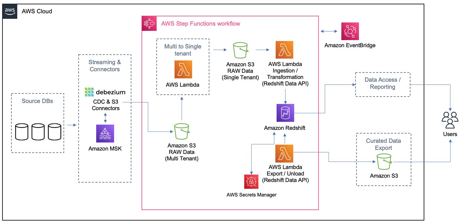
The main idea of this architecture is to be event-driven with eventual consistency. Any time new test cases or test results are created or modified, events trigger such that processing is immediate and new snapshot files are available via an API or data is pulled at the refresh frequency of the reporting or business intelligence (BI) tool. Every time the Amazon Simple Storage Service (Amazon S3) sink connector from Apache Kafka delivers a file on Amazon S3, Amazon EventBridge triggers an AWS Lambda function to transform the multi-tenant file into separated files, one per customer per table, and land it on specific folders on Amazon S3. As the files are created, another process is triggered to load the data from each customer on their schema or table on Amazon Redshift. On Amazon Redshift, materialized views were used to get the queries for the dashboards ready and easier to be returned to the Apache Superset. Also, the materialized views were configured to refresh automatically (with the autorefresh option), so Amazon Redshift updates the data automatically in the materialized views as soon as possible after base tables changes.
In the following sections, we detail specific implementation challenges and additional features required by customers discovered along the way.
Data export
As stated earlier, some customers want to get an export of their test data and create their data lake. For these customers, Tricentis provides incremental data as Apache Parquet files and will have the ability to filter on specific projects and specific date ranges. To ensure data integrity, Tricentis uses its technology known as Tosca DI (not part of the AWS Data Lab session).
Data security
The solution uses the following data security guardrails:
- Data isolation guardrails – Tricentis source databases systems are used by all customers, and therefore, data from different customers is in the same database. To isolate customer-specific data, Tricentis has a unique identifier that discriminates customer-specific data. All the queries filter data based on the discriminator to get customer-specific data. EventBridge triggers a Lambda function to transform multi-tenant files to single-tenant (customer) files to land in customer-specific S3 folders. Another Lambda function is triggered to load data from customer-specific folders to their specific schema in Amazon Redshift. The latter Lambda function is data isolation aware and triggers an alert and stops processing further for any data that doesn’t belong to a specific customer.
- Data access guardrails – To ensure access control, Tricentis applied role-based access control principles to users and service accounts for specific work-related resources. Access to Amazon Managed Streaming for Apache Kafka (Amazon MSK), Amazon S3, Amazon Relational Database Service (Amazon RDS), and Amazon Redshift was controlled by granting privileges at the role level and assigning those roles appropriate resources.
Pay per use and linear cost scalability
Tricentis’s objective is to pay for the compute and storage used and grow analytics infrastructure with linear cost scalability. To better manage storage costs in the data plane, Tricentis stores all raw and intermediate data in Amazon S3 storage in a compressed format. The Amazon MSK and Amazon Redshift is right-sized for Tricentis Analytics load and is allowed to scale up or down with no downtime based on future business needs. Data on all the stores, including Amazon MSK, Amazon Redshift, and Amazon S3, is subjected to tiered storage and retention policies per the customer data retention and archival requirements to reduce the cost further and provide linear cost scalability.
In the control plane, Debezium and Kafka Connect resources are turned on and off, so you only pay for what you use. Lambda triggers are triggered on an event or a schedule and turned off after completing tasks.
Automated data integrity
High data integrity is a fundamental design principle of Tricentis Analytics. Fortunately, Tricentis has a product called ToscaDI, which is used to automate the measurement of data integrity across many different data sources. The main idea is to use the machine-generated data type and log sequence number (LSN) to reflect the latest snapshot data from the change data capture (CDC) streams. Tricentis reached the data integrity automation milestone outside of the AWS Data Lab window by automatically triggering Tosca DI at various stages of the AWS serverless architecture (illustrated earlier), and because of that Tricentis was able to ensure expected record counts at every step, preventing data loss or inadvertent data manipulation. In future versions, Tricentis will have much deeper data integrity verification record counts and incorporate specific fields to ensure data quality (for example, nullness) and semantic or format validation. To date, the combination of CDC and data cleansing has resulted in ultra-high data integrity when comparing source data to the final Parquet file contents.
Performance and data loss prevention
Performance was tuned for maximum throughput at three stages in the pipeline:
- Data ingestion – Data integrity during ingestion was dramatically improved using CDC events and allowed us to rely on the well-respected replication mechanisms in PostgreSQL and Kafka, which simplified the system and eliminated a lot of the past data corrections that were in place. The Amazon S3 sink connector further streams data into Amazon S3 in real time by partitioning data into fixed-sized files. Fixed-size data files avoid further latency due to unbound file sizes. As a result, data was higher quality and was streamed in real time at a much faster rate.
- Data transformation – Batch processing is highly cost efficient and compute efficient, and can mitigate various potential performance issues if appropriately implemented. Tricentis uses batch transformation to move data from multi-tenant Amazon S3 to single-tenant Amazon S3 and between single-tenant Amazon S3 to Amazon Redshift by micro-batch loading. The batch processing is staged to work within the Lamba invocations limits and maximum Amazon Redshift connections limits to keep the cost minimum. However, the transformation pipeline is configurable to go real time by processing every incoming S3 file on an EventBridge event.
- Data queries – Materialized views with appropriate sort keys significantly improve the performance of repeated and predictable dashboard workloads. Tricentis pipelines use dynamic data loading in views and precomputed results in materialized views to seamlessly improve the performance of dashboards, along with setting up appropriate simple and compound sort keys to accelerate performance. Tricentis query performance is further accelerated by range-restricted predicates in sort keys.
Implementation challenges
Tricentis worked within the default limit of 1,000 concurrent Lambda function runs by keeping track of available functions at any given time and firing only those many functions for which slots are available. For the 10 GB memory limit per function, Tricentis right-sized the Amazon S3 sink connector generated files and single-tenant S3 files to not exceed 4 GB in size. The Lambda function throttling can be prevented by requesting a higher limit of concurrent runs if that becomes necessary later.
Tricentis also experienced some Amazon Redshift connection limitations. Amazon Redshift has quotas and adjustable quotas that limit the use of server resources. To effectively manage Amazon Redshift limits of maximum connections, Tricentis used connection pools to ensure optimal consumption and stability.
Results and next steps
The collaborative approach between Tricentis and the AWS Data Lab allowed considerable acceleration and the ability to meet timelines for establishing a big data solution that will benefit Tricentis customers for years. Since this writing, customer onboarding, observability and alerting, and security scanning were automated as part of a DevSecOps pipeline.
Within 6 weeks, the team was able to beta a data export service for one of Tricentis’ customers.
In the future, Tricentis anticipates adding multiple data sources, unify towards a common, ubiquitous language for testing data, and deliver richer insights so that our customers can have the correct data in a single view and increase confidence in their delivery of software at scale and speed.
Conclusion
In this post, we walked you through the journey the Tricentis team took with the AWS Data Lab during their participation in a Build Lab session. During the session, the Tricentis team and AWS Data Lab worked together to identify a best-fit architecture for their use cases and implement a prototype for delivering new insights for their customers.
To learn more about how the AWS Data Lab can help you turn your ideas into solutions, visit AWS Data Lab.
About the Authors
 Parag Doshi is Vice President of Engineering at Tricentis, where he continues to lead towards the vision of Innovation at the Speed of Imagination. He brings innovation to market by building world-class quality engineering SaaS such as qTest, the flagship test management product, and a new capability called Tricentis Analytics, which unlocks software development lifecycle insights across all types of testing. Prior to Tricentis, Parag was the founder of Anthem’s Cloud Platform Services, where he drove a hybrid cloud and DevSecOps capability and migrated 100 mission-critical applications. He enabled Anthem to build a new pharmacy benefits management business in AWS, resulting in $800 million in total operating gain for Anthem in 2020 per Forbes and CNBC. He also held posts at Hewlett-Packard, having multiple roles including Chief Technologist and head of architecture for DXC’s Virtual Private Cloud, and CTO for HP’s Application Services in the Americas region.
 Guru Havanur serves as a Principal, Big Data Engineering and Analytics team in Tricentis. Guru is responsible for data, analytics, development, integration with other products, security, and compliance activities. He strives to work with other Tricentis products and customers to improve data sharing, data quality, data integrity, and data compliance through the modern big data platform. With over 20 years of experience in data warehousing, a variety of databases, integration, architecture, and management, he thrives for excellence.
 Simon Guindon is an Architect at Tricentis. He has expertise in large-scale distributed systems and database consistency models, and works with teams in Tricentis around the world on scalability and high availability. You can follow his Twitter @simongui.
 Ricardo Serafim is a Senior AWS Data Lab Solutions Architect. With a focus on data pipelines, data lakes, and data warehouses, Ricardo helps customers create an end-to-end architecture and test an MVP as part of their path to production. Outside of work, Ricardo loves to travel with his family and watch soccer games, mainly from the “Timão” Sport Club Corinthians Paulista.
Modern applications are built with modular independent components or microservices that rely on an API framework to communicate with services. Many organizations are building data lakes to store and analyze large volumes of structured, semi-structured, and unstructured data. In addition, many teams are moving towards a data mesh architecture, which requires them to expose their data sets as easily consumable data products. To accomplish this on AWS, organizations use Amazon Simple Storage Service (Amazon S3) to provide cheap and reliable object storage to house their datasets. To enable interactive querying and analyzing their data in place using familiar SQL syntax, many teams are turning to Amazon Athena. Athena is an interactive query service that is used by modern applications to query large volumes of data on an S3 data lake using standard SQL.
When working with SQL databases, application developers and business analysts are most familiar with simple permissions management and synchronous query-response protocols—if a user has permissions to submit a query, they do so and receive the results from the server when the query is complete. Directly accessing Athena APIs, for example when integrating with a custom web application, requires an AWS Identity and Access Management (IAM) role for the applications, and requires you to build a custom process to poll for query completion asynchronously. The IAM role needs access to run Athena API calls, as well as S3 permissions to retrieve the Athena output stored on Amazon S3. Polling for Athena query completion when performed at several intervals could result in increased latency from the client perspective.
In this post, we present a solution that can integrate with your front-end application to query data from Amazon S3 using an Athena synchronous API invocation. With this solution, you can add a layer of abstraction to your application on direct Athena API calls and promote the access using the WebSocket API developed with Amazon API Gateway. The query results are returned back to the application as Amazon S3 presigned URLs.
Overview of solution
For illustration purposes, this post builds a COVID-19 data lake with a WebSocket API to handle Athena queries. Your application can invoke the WebSocket API to pull the data from Amazon S3 using an Athena SQL query, and the WebSocket API returns the JSON response with the presigned Amazon S3 URL. The application needs to parse the JSON message to read the presigned URL, download the data to local, and report the data back to the front end.
We use AWS Step Functions to poll the Athena query run. When the query is complete, Step Functions invokes an AWS Lambda function to generate the presigned URL and send the request back to the application.
The application doesn’t require direct access to Athena, just access to invoke the API. When using this solution, you should secure the API following AWS guidelines. For more information, refer to Controlling and managing access to a WebSocket API in API Gateway.
The following diagram summarizes the architecture, key components, and interactions in the solution.

The application is composed of the WebSocket API in API Gateway, which handles the connectivity between the client and Athena. A client application using the framework can submit the Athena SQL query and get back the presigned URL containing the query results data. The workflow includes the following steps:
- The application invokes the WebSocket API connection.
- A Lambda function is invoked to initiate the connection. The connection ID is stored in an Amazon DynamoDB
- When the client application is connected, it can invoke the
runqueryaction, which invokes the RunQuery Lambda function. - The function first runs the Athena query.
- When the query is started, the function checks the status and uses Step Functions to track the query progress.
- Step Functions invokes the third Lambda function to read the processed Athena results and get the presigned S3 URL. Failed messages are routed to an Amazon Simple Notification Service (Amazon SNS) topic, which you can subscribe to.
- The presigned URL is returned to the client application.
- The connection is closed using the OnDisconnect function.
The RunQuery Lambda function runs the Athena query using the start\_query\_execution request:
The Amazon S3 presigned URL is generated by invoking the generate\_presigned\_url request with the bucket and key information that hosts the Athena results. The code hard codes the presigner expiration to 120 seconds, which is configurable in the function input parameter PreSignerExpireSeconds. See the following code:
Prerequisites
This post assumes you have the following:
- Access to an AWS account
- Permissions to create an AWS CloudFormation stack
- Permissions to create the following resources:
- AWS Glue catalog databases and tables
- API Gateway
- Lambda function
- IAM roles
- Step Functions state machine
- SNS topic
- DynamoDB table
Enable the WebSocket API
To enable the WebSocket API of API Gateway, complete the following steps:
- Configure the Athena dataset.
To make the data from the AWS COVID-19 data lake available in the Data Catalog in your AWS account, create a CloudFormation stack using the following template. If you’re signed in to your AWS account, the following page fills out most of the stack creation form for you. All you need to do is choose Create stack. For instructions on creating a CloudFormation stack, see Getting started with AWS CloudFormation.
You can also use an existing Athena database to query, in which case you need to update the stack parameters.
- Sign in to the Athena console.
If this is the first time you’re using Athena, you must specify a query result location on Amazon S3. For more information about querying and accessing the data from Athena, see A public data lake for analysis of COVID-19 data.
- Configure the WebSocket framework using the following page, which deploys the API infrastructure using AWS Serverless Application Model (AWS SAM).
- Update the parameters
pBucketNamewith the S3 bucket (in theus-east-2region) that stores the Athena results and also update the database if you want to query an existing database. - Select the check box to acknowledge creation of IAM roles and choose Deploy.
At a high level, these are the primary resources deployed by the application template:
- An API Gateway with routes to the connect, disconnect, and query Lambda functions. Note that the API Gateway deployed with this sample doesn’t implement authentication and authorization. We recommend that you implement authentication and authorization before deploying into a production environment. Refer to Controlling and managing access to a WebSocket API in API Gateway to understand how to implement these security controls.
- A DynamoDB table for tracking client connections.
- Lambda functions to manage connection states using DynamoDB.
- A Lambda function to run the query and start the step function. The function includes an associated IAM role and policies with permissions to Step Functions, the AWS Glue Data Catalog, Athena, AWS Key Management Service (AWS KMS), and Amazon S3. Note that the Lambda execution role gives read access to the Data Catalog and S3 bucket that you specify in the deployment parameters. We recommend that you don’t include a catalog that contains sensitive data without first understanding the impacts and implementing additional security controls.
- A Lambda function with associated permissions to poll for the query results and return the presigned URL to the client.
- A Step Functions state machine with associated permissions to run the polling Lambda function and send API notifications using Amazon SNS.
Test the setup
To test the WebSocket API, you can use wscat, an open-source command line tool.
- Install NPM.
- Install wscat:
- On the console, connect to your published API endpoint by running the following command. The full URI to use can be found on the AWS CloudFormation console by finding the
WebSocketURIoutput in theserverlessrepo-aws-app-athena-websocket-integrationstack that was deployed by the AWS SAM application you deployed previously.
- To test the
runqueryfunction, send a JSON message like the following example. This triggers the state machine to run your SQL query using Athena and, using Lambda, return an S3 presigned URL to your client, which you can access to download the query results. Note that the API accepts any valid Athena query. Additional query validation could be added to the internal Lambda function if desired.
- Copy the value for
pre-signed-urland enter it into your browser window to access the results.
The presigned URL provides you temporary credentials to download the query results. For more information, refer to Using presigned URLs. This process can be integrated into a front-end web application to automatically download and display the results of the query.
Clean up
To avoid incurring ongoing charges, delete the resources you provisioned by deleting the CloudFormation stacks CovidLakeStacks and serverlessrepo-AthenaWebSocketIntegration via the AWS CloudFormation console. For detailed instructions, refer to the cleanup sections in the starter kit README files in the GitHub repo.
Conclusion
In this post, we showed how to integrate your application with Athena using the WebSocket API. We have included a GitHub repo for you to understand the code and modify it per your application requirements, to get the full benefits of the solution. We encourage you to further explore the features of the API Gateway WebSocket API to add in security using authorizers, view live invocations using dashboards, and expand the framework for more routes on action request.
Let’s stay in touch via the GitHub repo.
About the Authors
 Abhi Sodhani is a Sr. AI/ML Solutions Architect at AWS. He helps customers with a wide range of solutions, including machine leaning, artificial intelligence, data lakes, data warehousing, and data visualization. Outside of work, he is passionate about books, yoga, and travel.
 Robin Zimmerman is a Data and ML Engineer with AWS Professional Services. He works with AWS enterprise customers to develop systems to extract value from large volumes of data using AWS data, analytics, and machine learning services. When he’s not working, you’ll probably find him in the mountains—rock climbing, skiing, mountain biking, or out on whatever other adventure he can dream up.
Apache Iceberg is an open table format for very large analytic datasets, which captures metadata information on the state of datasets as they evolve and change over time. It adds tables to compute engines including Spark, Trino, PrestoDB, Flink, and Hive using a high-performance table format that works just like a SQL table. Iceberg has become very popular for its support for ACID transactions in data lakes and features like schema and partition evolution, time travel, and rollback.
Apache Iceberg integration is supported by AWS analytics services including Amazon EMR, Amazon Athena, and AWS Glue. Amazon EMR can provision clusters with Spark, Hive, Trino, and Flink that can run Iceberg. Starting with Amazon EMR version 6.5.0, you can use Iceberg with your EMR cluster without requiring a bootstrap action. In early 2022, AWS announced general availability of Athena ACID transactions, powered by Apache Iceberg. The recently released Athena query engine version 3 provides better integration with the Iceberg table format. AWS Glue 3.0 and later supports the Apache Iceberg framework for data lakes.
In this post, we discuss what customers want in modern data lakes and how Apache Iceberg helps address customer needs. Then we walk through a solution to build a high-performance and evolving Iceberg data lake on Amazon Simple Storage Service (Amazon S3) and process incremental data by running insert, update, and delete SQL statements. Finally, we show you how to performance tune the process to improve read and write performance.
How Apache Iceberg addresses what customers want in modern data lakes
More and more customers are building data lakes, with structured and unstructured data, to support many users, applications, and analytics tools. There is an increased need for data lakes to support database like features such as ACID transactions, record-level updates and deletes, time travel, and rollback. Apache Iceberg is designed to support these features on cost-effective petabyte-scale data lakes on Amazon S3.
Apache Iceberg addresses customer needs by capturing rich metadata information about the dataset at the time the individual data files are created. There are three layers in the architecture of an Iceberg table: the Iceberg catalog, the metadata layer, and the data layer, as depicted in the following figure (source).

The Iceberg catalog stores the metadata pointer to the current table metadata file. When a select query is reading an Iceberg table, the query engine first goes to the Iceberg catalog, then retrieves the location of the current metadata file. Whenever there is an update to the Iceberg table, a new snapshot of the table is created, and the metadata pointer points to the current table metadata file.
The following is an example Iceberg catalog with AWS Glue implementation. You can see the database name, the location (S3 path) of the Iceberg table, and the metadata location.

The metadata layer has three types of files: the metadata file, manifest list, and manifest file in a hierarchy. At the top of the hierarchy is the metadata file, which stores information about the table’s schema, partition information, and snapshots. The snapshot points to the manifest list. The manifest list has the information about each manifest file that makes up the snapshot, such as location of the manifest file, the partitions it belongs to, and the lower and upper bounds for partition columns for the data files it tracks. The manifest file tracks data files as well as additional details about each file, such as the file format. All three files work in a hierarchy to track the snapshots, schema, partitioning, properties, and data files in an Iceberg table.
The data layer has the individual data files of the Iceberg table. Iceberg supports a wide range of file formats including Parquet, ORC, and Avro. Because the Iceberg table tracks the individual data files instead of only pointing to the partition location with data files, it isolates the writing operations from reading operations. You can write the data files at any time, but only commit the change explicitly, which creates a new version of the snapshot and metadata files.
Solution overview
In this post, we walk you through a solution to build a high-performing Apache Iceberg data lake on Amazon S3; process incremental data with insert, update, and delete SQL statements; and tune the Iceberg table to improve read and write performance. The following diagram illustrates the solution architecture.

To demonstrate this solution, we use the Amazon Customer Reviews dataset in an S3 bucket (s3://amazon-reviews-pds/parquet/). In real use case, it would be raw data stored in your S3 bucket. We can check the data size with the following code in the AWS Command Line Interface (AWS CLI):
The total object count is 430, and total size is 47.4 GiB.
To set up and test this solution, we complete the following high-level steps:
- Set up an S3 bucket in the curated zone to store converted data in Iceberg table format.
- Launch an EMR cluster with appropriate configurations for Apache Iceberg.
- Create a notebook in EMR Studio.
- Configure the Spark session for Apache Iceberg.
- Convert data to Iceberg table format and move data to the curated zone.
- Run insert, update, and delete queries in Athena to process incremental data.
- Carry out performance tuning.
Prerequisites
To follow along with this walkthrough, you must have an AWS account with an AWS Identity and Access Management (IAM) role that has sufficient access to provision the required resources.
Set up the S3 bucket for Iceberg data in the curated zone in your data lake
Choose the Region in which you want to create the S3 bucket and provide a unique name:
Launch an EMR cluster to run Iceberg jobs using Spark
You can create an EMR cluster from the AWS Management Console, Amazon EMR CLI, or AWS Cloud Development Kit (AWS CDK). For this post, we walk you through how to create an EMR cluster from the console.
- On the Amazon EMR console, choose Create cluster.
- Choose Advanced options.
- For Software Configuration, choose the latest Amazon EMR release. As of January 2023, the latest release is 6.9.0. Iceberg requires release 6.5.0 and above.
- Select JupyterEnterpriseGateway and Spark as the software to install.
- For Edit software settings, select Enter configuration and enter
[{"classification":"iceberg-defaults","properties":{"iceberg.enabled":true}}]. - Leave other settings at their default and choose Next.

- For Hardware, use the default setting.
- Choose Next.
- For Cluster name, enter a name. We use
iceberg-blog-cluster. - Leave the remaining settings unchanged and choose Next.
- Choose Create cluster.
Create a notebook in EMR Studio
We now walk you through how to create a notebook in EMR Studio from the console.
- On the IAM console, create an EMR Studio service role.
- On the Amazon EMR console, choose EMR Studio.
- Choose Get started.
The Get started page appears in a new tab.
- Choose Create Studio in the new tab.
- Enter a name. We use iceberg-studio.
- Choose the same VPC and subnet as those for the EMR cluster, and the default security group.
- Choose AWS Identity and Access Management (IAM) for authentication, and choose the EMR Studio service role you just created.
- Choose an S3 path for Workspaces backup.
- Choose Create Studio.
- After the Studio is created, choose the Studio access URL.
- On the EMR Studio dashboard, choose Create workspace.
- Enter a name for your Workspace. We use
iceberg-workspace. - Expand Advanced configuration and choose Attach Workspace to an EMR cluster.
- Choose the EMR cluster you created earlier.
- Choose Create Workspace.
- Choose the Workspace name to open a new tab.
In the navigation pane, there is a notebook that has the same name as the Workspace. In our case, it is iceberg-workspace.
- Open the notebook.
- When prompted to choose a kernel, choose Spark.
Configure a Spark session for Apache Iceberg
Use the following code, providing your own S3 bucket name:
This sets the following Spark session configurations:
- spark.sql.catalog.demo – Registers a Spark catalog named demo, which uses the Iceberg Spark catalog plugin.
- spark.sql.catalog.demo.catalog-impl – The demo Spark catalog uses AWS Glue as the physical catalog to store Iceberg database and table information.
- spark.sql.catalog.demo.warehouse – The demo Spark catalog stores all Iceberg metadata and data files under the root path defined by this property:
s3://iceberg-curated-blog-data. - spark.sql.extensions – Adds support to Iceberg Spark SQL extensions, which allows you to run Iceberg Spark procedures and some Iceberg-only SQL commands (you use this in a later step).
- spark.sql.catalog.demo.io-impl – Iceberg allows users to write data to Amazon S3 through S3FileIO. The AWS Glue Data Catalog by default uses this FileIO, and other catalogs can load this FileIO using the io-impl catalog property.
Convert data to Iceberg table format
You can use either Spark on Amazon EMR or Athena to load the Iceberg table. In the EMR Studio Workspace notebook Spark session, run the following commands to load the data:
After you run the code, you should find two prefixes created in your data warehouse S3 path (s3://iceberg-curated-blog-data/reviews.db/all\_reviews): data and metadata.
Process incremental data using insert, update, and delete SQL statements in Athena
Athena is a serverless query engine that you can use to perform read, write, update, and optimization tasks against Iceberg tables. To demonstrate how the Apache Iceberg data lake format supports incremental data ingestion, we run insert, update, and delete SQL statements on the data lake.
Navigate to the Athena console and choose Query editor. If this is your first time using the Athena query editor, you need to configure the query result location to be the S3 bucket you created earlier. You should be able to see that the table reviews.all\_reviews is available for querying. Run the following query to verify that you have loaded the Iceberg table successfully:
Process incremental data by running insert, update, and delete SQL statements:
Performance tuning
In this section, we walk through different ways to improve Apache Iceberg read and write performance.
Configure Apache Iceberg table properties
Apache Iceberg is a table format, and it supports table properties to configure table behavior such as read, write, and catalog. You can improve the read and write performance on Iceberg tables by adjusting the table properties.
For example, if you notice that you write too many small files for an Iceberg table, you can config the write file size to write fewer but bigger size files, to help improve query performance.
| Property | Default | Description |
| write.target-file-size-bytes | 536870912 (512 MB) | Controls the size of files generated to target about this many bytes |
Use the following code to alter the table format:
Partitioning and sorting
To make a query run fast, the less data read the better. Iceberg takes advantage of the rich metadata it captures at write time and facilitates techniques such as scan planning, partitioning, pruning, and column-level stats such as min/max values to skip data files that don’t have match records. We walk you through how query scan planning and partitioning work in Iceberg and how we use them to improve query performance.
Query scan planning
For a given query, the first step in a query engine is scan planning, which is the process to find the files in a table needed for a query. Planning in an Iceberg table is very efficient, because Iceberg’s rich metadata can be used to prune metadata files that aren’t needed, in addition to filtering data files that don’t contain matching data. In our tests, we observed Athena scanned 50% or less data for a given query on an Iceberg table compared to original data before conversion to Iceberg format.
There are two types of filtering:
- Metadata filtering – Iceberg uses two levels of metadata to track the files in a snapshot: the manifest list and manifest files. It first uses the manifest list, which acts as an index of the manifest files. During planning, Iceberg filters manifests using the partition value range in the manifest list without reading all the manifest files. Then it uses selected manifest files to get data files.
- Data filtering – After selecting the list of manifest files, Iceberg uses the partition data and column-level stats for each data file stored in manifest files to filter data files. During planning, query predicates are converted to predicates on the partition data and applied first to filter data files. Then, the column stats like column-level value counts, null counts, lower bounds, and upper bounds are used to filter out data files that can’t match the query predicate. By using upper and lower bounds to filter data files at planning time, Iceberg greatly improves query performance.
Partitioning and sorting
Partitioning is a way to group records with the same key column values together in writing. The benefit of partitioning is faster queries that access only part of the data, as explained earlier in query scan planning: data filtering. Iceberg makes partitioning simple by supporting hidden partitioning, in the way that Iceberg produces partition values by taking a column value and optionally transforming it.
In our use case, we first run the following query on the Iceberg table not partitioned. Then we partition the Iceberg table by the category of the reviews, which will be used in the query WHERE condition to filter out records. With partitioning, the query could scan much less data. See the following code:
Run the following select statement on the non-partitioned all\_reviews table vs. the partitioned table to see the performance difference:
The following table shows the performance improvement of data partitioning, with about 50% performance improvement and 70% less data scanned.
| Dataset Name | Non-Partitioned Dataset | Partitioned Dataset |
| Runtime (seconds) | 8.20 | 4.25 |
| Data Scanned (MB) | 131.55 | 33.79 |
Note that the runtime is the average runtime with multiple runs in our test.
We saw good performance improvement after partitioning. However, this can be further improved by using column-level stats from Iceberg manifest files. In order to use the column-level stats effectively, you want to further sort your records based on the query patterns. Sorting the whole dataset using the columns that are often used in queries will reorder the data in such a way that each data file ends up with a unique range of values for the specific columns. If these columns are used in the query condition, it allows query engines to further skip data files, thereby enabling even faster queries.
Copy-on-write vs. read-on-merge
When implementing update and delete on Iceberg tables in the data lake, there are two approaches defined by the Iceberg table properties:
- Copy-on-write – With this approach, when there are changes to the Iceberg table, either updates or deletes, the data files associated with the impacted records will be duplicated and updated. The records will be either updated or deleted from the duplicated data files. A new snapshot of the Iceberg table will be created and pointing to the newer version of data files. This makes the overall writes slower. There might be situations that concurrent writes are needed with conflicts so retry has to happen, which increases the write time even more. On the other hand, when reading the data, there is no extra process needed. The query will retrieve data from the latest version of data files.
- Merge-on-read – With this approach, when there are updates or deletes on the Iceberg table, the existing data files will not be rewritten; instead new delete files will be created to track the changes. For deletes, a new delete file will be created with the deleted records. When reading the Iceberg table, the delete file will be applied to the retrieved data to filter out the delete records. For updates, a new delete file will be created to mark the updated records as deleted. Then a new file will be created for those records but with updated values. When reading the Iceberg table, both the delete and new files will be applied to the retrieved data to reflect the latest changes and produce the correct results. So, for any subsequent queries, an extra step to merge the data files with the delete and new files will happen, which will usually increase the query time. On the other hand, the writes might be faster because there is no need to rewrite the existing data files.
To test the impact of the two approaches, you can run the following code to set the Iceberg table properties:
Run the update, delete, and select SQL statements in Athena to show the runtime difference for copy-on-write vs. merge-on-read:
The following table summarizes the query runtimes.
| Query | Copy-on-Write | Merge-on-Read | ||||
| UPDATE | DELETE | SELECT | UPDATE | DELETE | SELECT | |
| Runtime (seconds) | 66.251 | 116.174 | 97.75 | 10.788 | 54.941 | 113.44 |
| Data scanned (MB) | 494.06 | 3.07 | 137.16 | 494.06 | 3.07 | 137.16 |
Note that the runtime is the average runtime with multiple runs in our test.
As our test results show, there are always trade-offs in the two approaches. Which approach to use depends on your use cases. In summary, the considerations come down to latency on the read vs. write. You can reference the following table and make the right choice.
| . | Copy-on-Write | Merge-on-Read |
| Pros | Faster reads | Faster writes |
| Cons | Expensive writes | Higher latency on reads |
| When to use | Good for frequent reads, infrequent updates and deletes or large batch updates | Good for tables with frequent updates and deletes |
Data compaction
If your data file size is small, you might end up with thousands or millions of files in an Iceberg table. This dramatically increases the I/O operation and slows down the queries. Furthermore, Iceberg tracks each data file in a dataset. More data files lead to more metadata. This in turn increases the overhead and I/O operation on reading metadata files. In order to improve the query performance, it’s recommended to compact small data files to larger data files.
When updating and deleting records in Iceberg table, if the read-on-merge approach is used, you might end up with many small deletes or new data files. Running compaction will combine all these files and create a newer version of the data file. This eliminates the need to reconcile them during reads. It’s recommended to have regular compaction jobs to impact reads as little as possible while still maintaining faster write speed.
Run the following data compaction command, then run the select query from Athena:
The following table compares the runtime before vs. after data compaction. You can see about 40% performance improvement.
| Query | Before Data Compaction | After Data Compaction |
| Runtime (seconds) | 97.75 | 32.676 seconds |
| Data scanned (MB) | 137.16 M | 189.19 M |
Note that the select queries ran on the all\_reviews table after update and delete operations, before and after data compaction. The runtime is the average runtime with multiple runs in our test.
Clean up
After you follow the solution walkthrough to perform the use cases, complete the following steps to clean up your resources and avoid further costs:
- Drop the AWS Glue tables and database from Athena or run the following code in your notebook:
- On the EMR Studio console, choose Workspaces in the navigation pane.
- Select the Workspace you created and choose Delete.
- On the EMR console, navigate to the Studios page.
- Select the Studio you created and choose Delete.
- On the EMR console, choose Clusters in the navigation pane.
- Select the cluster and choose Terminate.
- Delete the S3 bucket and any other resources that you created as part of the prerequisites for this post.
Conclusion
In this post, we introduced the Apache Iceberg framework and how it helps resolve some of the challenges we have in a modern data lake. Then we walked you though a solution to process incremental data in a data lake using Apache Iceberg. Finally, we had a deep dive into performance tuning to improve read and write performance for our use cases.
We hope this post provides some useful information for you to decide whether you want to adopt Apache Iceberg in your data lake solution.
About the Authors
 Flora Wu is a Sr. Resident Architect at AWS Data Lab. She helps enterprise customers create data analytics strategies and build solutions to accelerate their businesses outcomes. In her spare time, she enjoys playing tennis, dancing salsa, and traveling.
 Daniel Li is a Sr. Solutions Architect at Amazon Web Services. He focuses on helping customers develop, adopt, and implement cloud services and strategy. When not working, he likes spending time outdoors with his family.
Amazon Redshift is a fully managed, petabyte-scale data warehouse service in the cloud. Amazon Redshift enables you to use SQL for analyzing structured and semi-structured data with best price performance along with secure access to the data.
As more users start querying data in a data warehouse, access control is paramount to protect valuable organizational data. Database administrators want to continuously monitor and manage user privileges to maintain proper data access in the data warehouse. Amazon Redshift provides granular access control on the database, schema, table, column, row, and other database objects by granting privileges to roles, groups, and users from a SQL interface. To monitor privileges configured in Amazon Redshift, you can retrieve them by querying system tables.
Although Amazon Redshift provides a broad capability of managing access to database objects, we have heard from customers that they want to visualize and monitor privileges without using a SQL interface. In this post, we introduce predefined dashboards using Grafana which visualizes database privileges without writing SQL. This dashboard will help database administrators to reduce the time spent on database administration and increase the frequency of monitoring cycles.
Database security in Amazon Redshift
Security is the top priority at AWS. Amazon Redshift provides four levels of control:
- Cluster management
- Cluster connectivity
- Database access
- Temporary database credentials and single sign-on
This post focuses on database access, which relates to user access control against database objects. For more information, see Managing database security.
Amazon Redshift uses the GRANT command to define permissions in the database. For most database objects, GRANT takes three parameters:
- Identity – The entity you grant access to. This could be a user, role, or group.
- Object – The type of database object. This could be a database, schema, table or view, column, row, function, procedure, language, datashare, machine leaning (ML) model, and more.
- Privilege – The type of operation. Examples include CREATE, SELECT, ALTER, DROP, DELETE, and INSERT. The level of privilege depends on the object.
To remove access, use the REVOKE command.
Additionally, Amazon Redshift offers granular access control with the Row-level security (RLS) feature. You can attach or detach RLS policies to identities with the ATTACH RLS POLICY and DETACH RLS POLICY commands, respectively. See RLS policy ownership and management for more details.
Generally, database administrator monitors and reviews the identities, objects, and privileges periodically to ensure proper access is configured. They also need to investigate access configurations if database users face permission errors. These tasks require a SQL interface to query multiple system tables, which can be a repetitive and undifferentiated operation. Therefore, database administrators need a single pane of glass to quickly navigate through identities, objects, and privileges without writing SQL.
Solution overview
The following diagram illustrates the solution architecture and its key components:
- Amazon Redshift contains database privilege information in system tables.
- Grafana provides a predefined dashboard to visualize database privileges. The dashboard runs queries against the Amazon Redshift system table via the Amazon Redshift Data API.
Note that the dashboard focuses on visualization. SQL interface is required to configure privileges in Amazon Redshift. You can use query editor v2, a web-based SQL interface which enables users to run SQL commands from a browser.
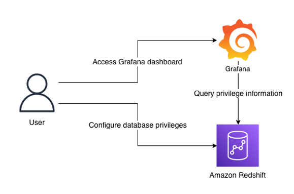
Prerequisites
Before moving to the next section, you should have the following prerequisites:
- An AWS account
- Create an Amazon Redshift cluster
- Setup Amazon Managed Grafana or local Grafana
- To setup with Amazon Managed Grafana, go through the following sections in Query and visualize Amazon Redshift operational metrics using the Amazon Redshift plugin for Grafana:
- Configure an Amazon Redshift cluster
- Configure an Amazon Managed Grafana workspace and sign in to Grafana
- Create a database user for Amazon Managed Grafana
- Configure a user in AWS SSO for Amazon Managed Grafana UI access
- Configure an Amazon Managed Grafana workspace and sign in to Grafana
- Set up an Amazon Redshift data source in Grafana
- To setup with local Grafana, first install Grafana following the official setup documentation. Next, go through the following sections in Query and visualize Amazon Redshift operational metrics using the Amazon Redshift plugin for Grafana:
- Create a database user for Amazon Managed Grafana
- Set up an Amazon Redshift data source in Grafana
- To setup with Amazon Managed Grafana, go through the following sections in Query and visualize Amazon Redshift operational metrics using the Amazon Redshift plugin for Grafana:
While Amazon Managed Grafana controls the plugin version and updates periodically, local Grafana allows user to control the version. Therefore, local Grafana could be an option if you need earlier access for the latest features. Refer to plugin changelog for released features and versions.
Import the dashboards
After you have finished the prerequisites, you should have access to Grafana configured with Amazon Redshift as a data source. Next, import two dashboards for visualization.
- In Grafana console, go to the created Redshift data source and click Dashboards
- Import the Amazon Redshift Identities and Objects
- Go to the data source again and import the Amazon Redshift Privileges
Each dashboard will appear once imported.
Amazon Redshift Identities and Objects dashboard
The Amazon Redshift Identities and Objects dashboard shows identites and database objects in Amazon Redshift, as shown in the following screenshot.
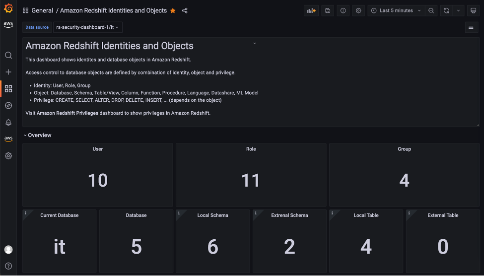
The Identities section shows the detail of each user, role, and group in the source database.
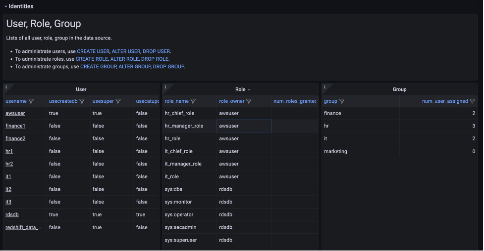
One of the key features in this dashboard is the Role assigned to Role, User section, which uses a node graph panel to visualize the hierarchical structure of roles and users from multiple system tables. This visualization can help administrators quickly examine which roles are inherited to users instead of querying multiple system tables. For more information about role-based access, refer to Role-based access control (RBAC).
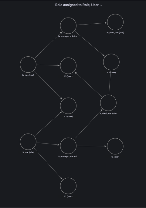
Amazon Redshift Privileges dashboard
The Amazon Redshift Privileges dashboard shows privileges defined in Amazon Redshift.
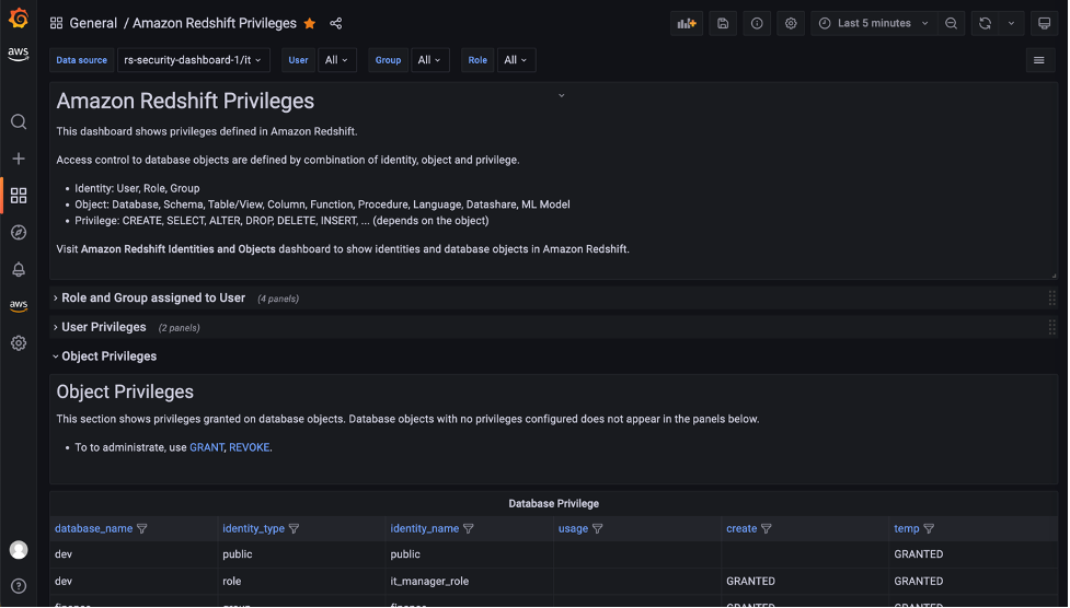
In the Role and Group assigned to User section, open the Role assigned to User panel to list the roles for a specific user. In this panel, you can list and compare roles assigned to multiple users. Use the User drop-down at the top of the dashboard to select users.

The dashboard will refresh immediately and show filtered result for selected users. Following screenshot is the filtered result for user hr1, hr2 and it3.
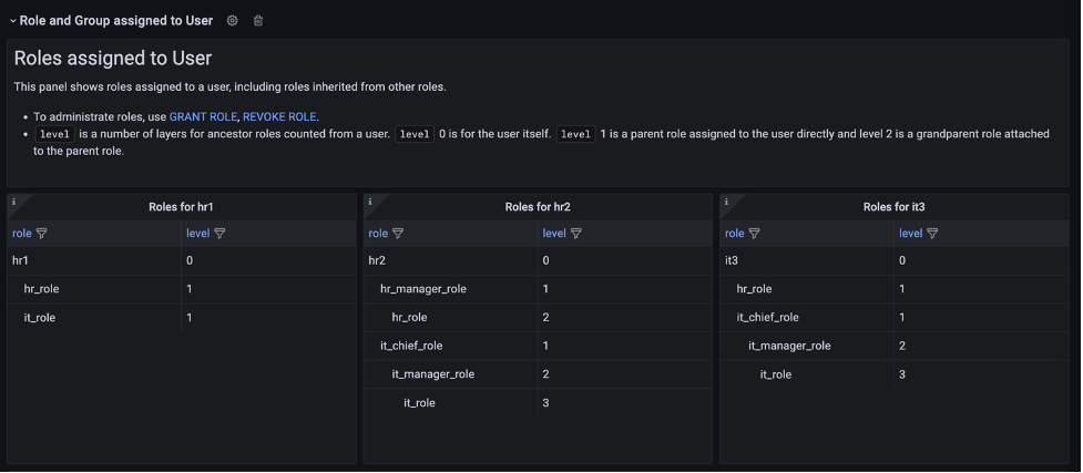
The Object Privileges section shows the privileges granted for each database object and identity. Note that objects with no privileges granted are not listed here. To show the full list of database objects, use the Amazon Redshift Identities and Objects dashboard.
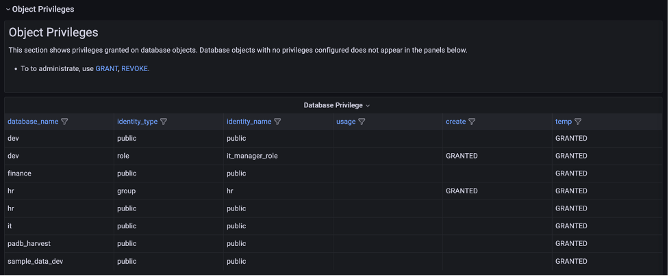
The Object Privileges (RLS) section contains visualizations for row-level security (RLS). The Policy attachments panel enables you to examine RLS configuration by visualizing relation between of tables, policies, roles and users.
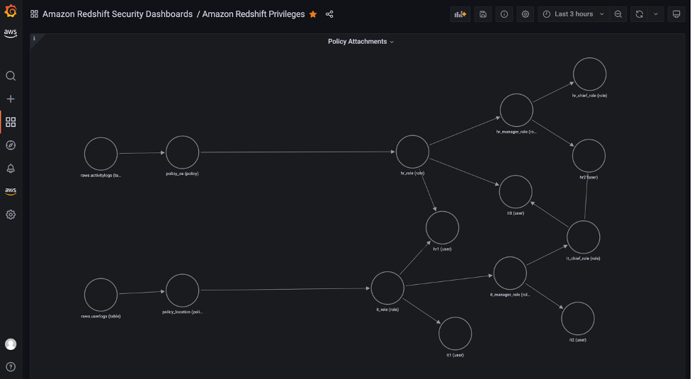
Conclusion
In this post, we introduced a visualization for database privileges of Amazon Redshift using predefined Grafana dashboards. Database administrators can use these dashboards to quickly navigate through identities, objects, and privileges without writing SQL. You can also customize the dashboard to meet your business requirements. The JSON definition file of this dashboard is maintained as part of OSS in the Redshift data source for Grafana GitHub repository.
For more information about the topics described to in this post, refer to the following:
- Redshift data source for Grafana document
- Redshift data source for Grafana GitHub repository
- Monitor all your Redshift clusters in Grafana with the new Amazon Redshift data source plugin
- Query and visualize Amazon Redshift operational metrics using the Amazon Redshift plugin for Grafana
About the author

Yota Hamaoka is an Analytics Solution Architect at Amazon Web Services. He is focused on driving customers to accelerate their analytics journey with Amazon Redshift.
Finding similar columns in a data lake has important applications in data cleaning and annotation, schema matching, data discovery, and analytics across multiple data sources. The inability to accurately find and analyze data from disparate sources represents a potential efficiency killer for everyone from data scientists, medical researchers, academics, to financial and government analysts.
Conventional solutions involve lexical keyword search or regular expression matching, which are susceptible to data quality issues such as absent column names or different column naming conventions across diverse datasets (for example, zip\_code, zcode, postalcode).
In this post, we demonstrate a solution for searching for similar columns based on column name, column content, or both. The solution uses approximate nearest neighbors algorithms available in Amazon OpenSearch Service to search for semantically similar columns. To facilitate the search, we create features representations (embeddings) for individual columns in the data lake using pre-trained Transformer models from the sentence-transformers library in Amazon SageMaker. Finally, to interact with and visualize results from our solution, we build an interactive Streamlit web application running on AWS Fargate.
We include a code tutorial for you to deploy the resources to run the solution on sample data or your own data.
Solution overview
The following architecture diagram illustrates the two-stage workflow for finding semantically similar columns. The first stage runs an AWS Step Functions workflow that creates embeddings from tabular columns and builds the OpenSearch Service search index. The second stage, or the online inference stage, runs a Streamlit application through Fargate. The web application collects input search queries and retrieves from the OpenSearch Service index the approximate k-most-similar columns to the query.

Figure 1. Solution architecture
The automated workflow proceeds in the following steps:
- The user uploads tabular datasets into an Amazon Simple Storage Service (Amazon S3) bucket, which invokes an AWS Lambda function that initiates the Step Functions workflow.
- The workflow begins with an AWS Glue job that converts the CSV files into Apache Parquet data format.
- A SageMaker Processing job creates embeddings for each column using pre-trained models or custom column embedding models. The SageMaker Processing job saves the column embeddings for each table in Amazon S3.
- A Lambda function creates the OpenSearch Service domain and cluster to index the column embeddings produced in the previous step.
- Finally, an interactive Streamlit web application is deployed with Fargate. The web application provides an interface for the user to input queries to search the OpenSearch Service domain for similar columns.
You can download the code tutorial from GitHub to try this solution on sample data or your own data. Instructions on the how to deploy the required resources for this tutorial are available on Github.
Prerequistes
To implement this solution, you need the following:
- An AWS account.
- Basic familiarity with AWS services such as the AWS Cloud Development Kit (AWS CDK), Lambda, OpenSearch Service, and SageMaker Processing.
- A tabular dataset to create the search index. You can bring your own tabular data or download the sample datasets on GitHub.
Build a search index
The first stage builds the column search engine index. The following figure illustrates the Step Functions workflow that runs this stage.

Figure 2 – Step functions workflow – multiple embedding models
Datasets
In this post, we build a search index to include over 400 columns from over 25 tabular datasets. The datasets originate from the following public sources:
s3://sagemaker-sample-files/datasets/tabular/- NYC Open Data
- Chicago Data Portal
For the the full list of the tables included in the index, see the code tutorial on GitHub.
You can bring your own tabular dataset to augment the sample data or build your own search index. We include two Lambda functions that initiate the Step Functions workflow to build the search index for individual CSV files or a batch of CSV files, respectively.
Transform CSV to Parquet
Raw CSV files are converted to Parquet data format with AWS Glue. Parquet is a column-oriented format file format preferred in big data analytics that provides efficient compression and encoding. In our experiments, the Parquet data format offered significant reduction in storage size compared to raw CSV files. We also used Parquet as a common data format to convert other data formats (for example JSON and NDJSON) because it supports advanced nested data structures.
Create tabular column embeddings
To extract embeddings for individual table columns in the sample tabular datasets in this post, we use the following pre-trained models from the sentence-transformers library. For additional models, see Pretrained Models.
| Model name | Dimension | Size (MB) |
| all-MiniLM-L6-v2 | 384 | 80 |
| all-distilroberta-v1 | 768 | 290 |
| average\_word\_embeddings\_glove.6B.300d | 300 | 420 |
The SageMaker Processing job runs create\_embeddings.py(code) for a single model. For extracting embeddings from multiple models, the workflow runs parallel SageMaker Processing jobs as shown in the Step Functions workflow. We use the model to create two sets of embeddings:
- column\_name\_embeddings – Embeddings of column names (headers)
- column\_content\_embeddings – Average embedding of all the rows in the column
For more information about the column embedding process, see the code tutorial on GitHub.
An alternative to the SageMaker Processing step is to create a SageMaker batch transform to get column embeddings on large datasets. This would require deploying the model to a SageMaker endpoint. For more information, see Use Batch Transform.
Index embeddings with OpenSearch Service
In the final step of this stage, a Lambda function adds the column embeddings to a OpenSearch Service approximate k-Nearest-Neighbor (kNN) search index. Each model is assigned its own search index. For more information about the approximate kNN search index parameters, see k-NN.
Online inference and semantic search with a web app
The second stage of the workflow runs a Streamlit web application where you can provide inputs and search for semantically similar columns indexed in OpenSearch Service. The application layer uses an Application Load Balancer, Fargate, and Lambda. The application infrastructure is automatically deployed as part of the solution.
The application allows you to provide an input and search for semantically similar column names, column content, or both. Additionally, you can select the embedding model and number of nearest neighbors to return from the search. The application receives inputs, embeds the input with the specified model, and uses kNN search in OpenSearch Service to search indexed column embeddings and find the most similar columns to the given input. The search results displayed include the table names, column names, and similarity scores for the columns identified, as well as the locations of the data in Amazon S3 for further exploration.
The following figure shows an example of the web application. In this example, we searched for columns in our data lake that have similar Column Names (payload type) to district (payload). The application used all-MiniLM-L6-v2 as the embedding model and returned 10 (k) nearest neighbors from our OpenSearch Service index.
The application returned transit\_district, city, borough, and location as the four most similar columns based on the data indexed in OpenSearch Service. This example demonstrates the ability of the search approach to identify semantically similar columns across datasets.

Figure 3: Web application user interface
Clean up
To delete the resources created by the AWS CDK in this tutorial, run the following command:
cdk destroy --allConclusion
In this post, we presented an end-to-end workflow for building a semantic search engine for tabular columns.
Get started today on your own data with our code tutorial available on GitHub. If you’d like help accelerating your use of ML in your products and processes, please contact the Amazon Machine Learning Solutions Lab.
About the Authors
 Kachi Odoemene is an Applied Scientist at AWS AI. He builds AI/ML solutions to solve business problems for AWS customers.
 Taylor McNally is a Deep Learning Architect at Amazon Machine Learning Solutions Lab. He helps customers from various industries build solutions leveraging AI/ML on AWS. He enjoys a good cup of coffee, the outdoors, and time with his family and energetic dog.
 Austin Welch is a Data Scientist in the Amazon ML Solutions Lab. He develops custom deep learning models to help AWS public sector customers accelerate their AI and cloud adoption. In his spare time, he enjoys reading, traveling, and jiu-jitsu.
Amazon Managed Streaming for Apache Kafka (Amazon MSK) is an event streaming platform that you can use to build asynchronous applications by decoupling producers and consumers. Monitoring of different Amazon MSK metrics is critical for efficient operations of production workloads. Amazon MSK gathers Apache Kafka metrics and sends them to Amazon CloudWatch, where you can view them. You can also monitor Amazon MSK with Prometheus, an open-source monitoring application. Many of our customers use such open-source monitoring tools like Prometheus and Grafana, but doing it in self-managed environment comes with its own challenges regarding manageability, availability, and security.
In this post, we show how you can build an AWS Cloud native monitoring platform for Amazon MSK using the fully managed, highly available, scalable, and secure services Amazon Managed service for Prometheus and Amazon Managed Grafana for better operational insights.
Why is Kafka monitoring critical?
As a critical component of the IT infrastructure, it is necessary to track Amazon MSK clusters’ operations and their efficiencies. Amazon MSK metrics helps monitor critical tasks while operating applications. You can not only troubleshoot problems that have already occurred, but also discover anomalous behavior patterns and prevent problems from occurring in the first place.
Some customers currently use various third-party monitoring solutions like lenses.io, AppDynamics, Splunk, and others to monitor Amazon MSK operational metrics. In the context of cloud computing, customers are looking for an AWS Cloud native service that offers equivalent or better capabilities but with the added advantage of being highly scalable, available, secure, and fully managed.
Amazon MSK clusters emit a very large number of metrics via JMX, many of which can be useful for tuning the performance of your cluster, producers, and consumers. However, that large volume brings complexity with monitoring. By default, Amazon MSK clusters come with CloudWatch monitoring of your essential metrics. You can extend your monitoring capabilities by using open-source monitoring with Prometheus. This feature enables you to scrape a Prometheus friendly API to gather all the JMX metrics and work with the data in Prometheus.
This solution provides a simple and easy observability platform for Amazon MSK along with much needed insights into various critical operational metrics that yields the following organizational benefits for your IT operations or application teams:
- You can quickly drill down to various Amazon MSK components (broker level, topic level, or cluster level) and identify issues that need investigation
- You can investigate Amazon MSK issues after the event using the historical data in Amazon Managed Service for Prometheus
- You can shorten or eliminate long calls that waste time questioning business users on Amazon MSK issues
In this post, we set up Amazon Managed Service for Prometheus, Amazon Managed Grafana, and a Prometheus server running as container on Amazon Elastic Compute Cloud (Amazon EC2) to provide a fully managed monitoring solution for Amazon MSK.
The solution provides an easy-to-configure dashboard in Amazon Managed Grafana for various critical operation metrics, as demonstrated in the following video.
Solution overview
Amazon Managed Service for Prometheus reduces the heavy lifting required to get started with monitoring applications across Amazon MSK, Amazon Elastic Kubernetes Service (Amazon EKS), Amazon Elastic Container Service (Amazon ECS), and AWS Fargate, as well as self-managed Kubernetes clusters. The service also seamlessly integrates with Amazon Managed Grafana to simplify data visualization, team management authentication, and authorization.
Grafana empowers you to create dashboards and alerts from multiple sources such as an Amazon Managed Prometheus workspace, CloudWatch, AWS X-Ray, Amazon OpenSearch Service, Amazon Redshift, and Amazon Timestream.
The following diagram demonstrates the solution architecture. This solution deploys a Prometheus server running as a container within Amazon EC2, which constantly scrapes metrics from the MSK brokers and remote write metrics to an Amazon Managed Service for Prometheus workspace. As of this writing, Amazon Managed Service for Prometheus is not able to scrape the metrics directly, therefore a Prometheus server is necessary to do so. We use Amazon Managed Grafana to query and visualize the operational metrics for the Amazon MSK platform.

The following are the high-level steps to deploy the solution:
- Create an EC2 key pair.
- Configure your Amazon MSK cluster and associated resources. We demonstrate how to configure an existing Amazon MSK cluster or create a new one.
- Option A:- Modify an existing Amazon MSK cluster
- Option B:- Create a new Amazon MSK cluster
- Enable AWS IAM Identity Center (successor to AWS Single Sign-On), if not enabled.
- Configure Amazon Managed Grafana and Amazon Managed Service for Prometheus.
- Configure Prometheus and start the service.
- Configure the data sources in Amazon Managed Grafana.
- Import the Grafana dashboard.
Prerequisites
- Clone the GitHub repository to download the AWS CloudFormation template files:
- You download three CloudFormation template files along with the Prometheus configuration file (
prometheus.yml),targets.jsonfile (you need this to update the MSK broker DNS later on), and three JSON files for creating a dashboard within Amazon Managed Grafana. - Make sure internet connection is allowed to download docker image of Prometheus from within Prometheus server
1. Create an EC2 key pair
To create your EC2 key pair, complete the following steps:
- On the Amazon EC2 console, under Network & Security in the navigation pane, choose Key Pairs.
- Choose Create key pair.
- For Name, enter
DemoMSKKeyPair. - For Key pair type¸ select RSA.
- For Private key file format, choose the format in which to save the private key:
- To save the private key in a format that can be used with OpenSSH, select .pem.
- To save the private key in a format that can be used with PuTTY, select .ppk.

The private key file is automatically downloaded by your browser. The base file name is the name that you specified as the name of your key pair, and the file name extension is determined by the file format that you chose.
- Save the private key file in a safe place.
2. Configure your Amazon MSK cluster and associated resources.
Using the following options to configure an existing Amazon MSK cluster or create a new one.
2.a Modify an existing Amazon MSK cluster
If you want to create a new Amazon MSK cluster for this solution, skip to the section – 2.b.Create a new Amazon MSK cluster, otherwise complete the steps in this section to modify an existing cluster.
Validate cluster monitoring settings
We must enable enhanced partition-level monitoring (available at an additional cost) and open monitoring with Prometheus. Note that open monitoring with Prometheus is only available for provisioned mode clusters.
- Sign in to the account where the Amazon MSK cluster is that you want to monitor.
- Open your Amazon MSK cluster.
- On the Properties tab, navigate to Monitoring metrics.
- Check the monitoring level for Amazon CloudWatch metrics for this cluster, and choose Edit to edit the cluster.
- Select Enhance partition-level monitoring.

- Check the monitoring label for Open monitoring with Prometheus, and choose Edit to edit the cluster.
- Select Enable open monitoring for Prometheus.
- Under Prometheus exporters, select JMX Exporter and Note Exporter.

- Under Broker log delivery, select Deliver to Amazon CloudWatch Logs.
- For Log group, enter your log group for Amazon MSK.
- Choose Save changes.
Deploy CloudFormation stack
Now we deploy the CloudFormation stack Prometheus\_Cloudformation.yml that we downloaded earlier.
- On the AWS CloudFormation console, choose Stacks in the navigation pane.
- Choose Create stack.
- For Prepare template, select Template is ready.
- For Template source, select Upload a template.
- Upload the
Prometheus\_Cloudformation.ymlfile, then choose Next.

- For Stack name, enter
Prometheus. - VPCID – Provide the VPC ID where your Amazon MSK cluster is deployed (mandatory)
- VPCCIdr – Provide the VPC CIDR where your Amazon MSK Cluster is deployed (mandatory)
- SubnetID – Provide any one of the subnets ID where your existing Amazon MSK cluster is deployed (mandatory)
- MSKClusterName – Provide the name your existing Amazon MSK Cluster
- Leave Cloud9InstanceType, KeyName, and LatestAmild as default.
- Choose Next.

- On the Review page, select I acknowledge that AWS CloudFormation might create IAM resources.
- Choose Create stack.
You’re redirected to the AWS CloudFormation console, and can see the status as CREATE\_IN\_PROGRESSS. Wait until the status changes to COMPLETE.

- On the stack’s Outputs tab, note the values for the following keys (if you don’t see anything under Outputs tab, click on refresh icon):
PrometheusInstancePrivateIPPrometheusSecurityGroupId

Update the Amazon MSK cluster security group
Complete the following steps to update the security group of the existing Amazon MSK cluster to allow communication from the Kafka client and Prometheus server:
- On the Amazon MSK console, navigate to your Amazon MSK cluster.
- On the Properties tab, under Network settings, open the security group.
- Choose Edit inbound rules.
- Choose Add rule and create your rule with the following parameters:
- Type – Custom TCP
- Port range – 11001–11002
- Source – The Prometheus server security group ID
Set up your AWS Cloud9 environment
To configure your AWS Cloud9 environment, complete the following steps:
- On the AWS Cloud9 console, choose Environments in the navigation pane.
- Select
Cloud9EC2Bastionand choose Open in Cloud9.

- Close the Welcome tab and open a new terminal tab
- Create an SSH key file with the contents from the private key file
DemoMSKKeyPairusing the following command: - Run the following command to list the newly created key file
- Open the file, enter the contents of the private key file
DemoMSKKeyPair, then save the file.

- Change the permissions of the file using the following command:
- Log in to the Prometheus server using this key file and the private IP noted earlier:
- Once you’re logged in, check if the Docker service is up and running using the following command:

- To exit the server, enter
exitand press Enter.
2.b Create a new Amazon MSK cluster
If you don’t have an Amazon MSK cluster running in your environment, or you don’t want to use an existing cluster for this solution, complete the steps in this section.
As part of these steps, your cluster will have the following properties:
- An AWS Identity and Access Management (IAM) role used to control who can perform Amazon MSK operations on your cluster
- TLS encryption between the client and brokers
- TLS encryption within the cluster
- An AWS Key Management Service (AWS KMS) managed key for encryption at rest
Deploy CloudFormation stack
Complete the following steps to deploy the CloudFormation stack MSKResource\_Cloudformation.yml:
- On the AWS CloudFormation console, choose Stacks in the navigation pane.
- Choose Create stack.
- For Prepare template, select Template is ready.
- For Template source, select Upload a template.
- Upload the
MSKResource\_Cloudformation.ymlfile, then choose Next. - For Stack name, enter
MSKDemo. - Network Configuration – Generic (mandatory)
- Stack to be deployed in NEW VPC? (true/false) – if false, you MUST provide VPCCidr and other details under Existing VPC section (Default is true)
- VPCCidr – Default is 10.0.0.0/16 for a new VPC. You can have any valid values as per your environment. If deploying in an existing VPC, provide the CIDR for the same
- Network Configuration – For New VPC
- PrivateSubnetMSKOneCidr (Default is 10.0.1.0/24)
- PrivateSubnetMSKTwoCidr (Default is 10.0.2.0/24)
- PrivateSubnetMSKThreeCidr (Default is 10.0.3.0/24)
- PublicOneCidr (Default is 10.0.0.0/24)
- Network Configuration – For Existing VPC (You need at least 4 subnets)
- VpcId – Provide the value if you are using any existing VPC to deploy the resources else leave it blank(default)
- SubnetID1 – Any one of the existing subnets from the given VPCID
- SubnetID2 – Any one of the existing subnets from the given VPCID
- SubnetID3 – Any one of the existing subnets from the given VPCID
- PublicSubnetID – Any one of the existing subnets from the given VPCID
- Leave the remaining parameters as default and choose Next.

- On the Review page, select I acknowledge that AWS CloudFormation might create IAM resources.
- Choose Create stack.
You’re redirected to the AWS CloudFormation console, and can see the status as CREATE\_IN\_PROGRESSS. Wait until the status changes to COMPLETE.

- On the stack’s Outputs tab, note the values for the following (if you don’t see anything under Outputs tab, click on refresh icon):
KafkaClientPrivateIPPrometheusInstancePrivateIP
Set up your AWS Cloud9 environment
Follow the steps as outlined in the previous section to configure your AWS Cloud9 environment.
Retrieve the cluster broker list
To get your MSK cluster broker list, complete the following steps:
- On the Amazon MSK console, navigate to your cluster.
- In the Cluster summary section, choose View client information.
- In the Bootstrap servers section, copy the private endpoint.
You need this value to perform some operations later, such as creating an MSK topic, producing sample messages, and consuming those sample messages.
- Choose Done.
- On the Properties tab, in the Brokers details section, note the endpoints listed.
These need to be updated in the targets.json file (used for Prometheus configuration in a later step).
3. Enable IAM Identity Center
Before you deploy the CloudFormation stack for Amazon Managed Service for Prometheus and Amazon Managed Grafana, make sure to enable IAM Identity Center.
If you don’t use IAM Identity Center, alternatively, you can set up user authentication via SAML. For more information, refer to Using SAML with your Amazon Managed Grafana workspace.
If IAM Identity Center is currently enabled/configured in another region, you don’t need to enable in your current region.
Complete the following steps to enable IAM Identity Center:
- On the IAM Identity Center console, under Enable IAM Identity Center, choose Enable.

- Choose Create AWS organization.
4. Configure Amazon Managed Grafana and Amazon Managed Service for Prometheus
Complete the steps in this section to set up Amazon Managed Service for Prometheus and Amazon Managed Grafana.
Deploy CloudFormation template
Complete the following steps to deploy the CloudFormation stack AMG\_AMP\_Cloudformation:
- On the AWS CloudFormation console, choose Stacks in the navigation pane.
- Choose Create stack.
- For Prepare template, select Template is ready.
- For Template source, select Upload a template.
- Upload the
AMG\_AMP\_Cloudformation.ymlfile, then choose Next. - For Stack name, enter ManagedPrometheusAndGrafanaStack, then choose Next.
- On the Review page, select I acknowledge that AWS CloudFormation might create IAM resources.
- Choose Create stack.
You’re redirected to the AWS CloudFormation console, and can see the status as CREATE\_IN\_PROGRESSS. Wait until the status changes to COMPLETE.
- On the stack’s Outputs tab, note the values for the following (if you don’t see anything under Outputs tab, click on refresh icon):
- GrafanaWorkspaceURL – This is Amazon Managed Grafana URL
- PrometheusEndpointWriteURL – This is the Amazon Managed Service for Prometheus write endpoint URL

Create a user for Amazon Managed Grafana
Complete the following steps to create a user for Amazon Managed Grafana:
- On the IAM Identity Center console, choose Users in the navigation pane.
- Choose Add user.
- For Username, enter
grafana-admin. - Enter and confirm your email address to receive a confirmation email.

- Skip the optional steps, then choose Add user.
A success message appears at the top of the console.
- In the confirmation email, choose Accept invitation and set your user password.

- On the Amazon Managed Grafana console, choose Workspaces in the navigation pane.
- Open the workspace
Amazon-Managed-Grafana. - Make a note of the Grafana workspace URL.
You use this URL to log in to view your Grafana dashboards.
- On the Authentication tab, choose Assign new user or group.

- Select the user you created earlier and choose Assign users and groups.

- On the Action menu, choose what kind of user to make it: admin, editor, or viewer.
Note that your Grafana workspace needs as least one admin user.
- Navigate to the Grafana URL you copied earlier in your browser.
- Choose Sign in with AWS IAM Identity Center.

- Log in with your IAM Identity Center credentials.
5. Configure Prometheus and start the service
When you cloned the GitHub repo, you downloaded two configuration files: prometheus.yml and targets.json. In this section, we configure these two files.
- Use any IDE (Visual Studio Code or Notepad++) to open prometheus.yml.
- In the
remote\_write section, update the remote write URL and Region.

- Use any IDE to open
targets.json. - Update the targets with the broker endpoints you obtained earlier.

- In your AWS Cloud9 environment, choose File, then Upload Local Files.
- Choose Select Files and upload targets.json and prometheus.yml from your local machine.

- In the AWS Cloud9 environment, run the following command using the key file you created earlier:
- copy targets.json to the Prometheus server:
- copy prometheus.yml to the Prometheus server:
- SSH into the Prometheus server and start the container service for Prometheus
- start the prometheus container
- Check if the Docker service is running:

6. Configure data sources in Amazon Managed Grafana
To configure your data sources, complete the following steps:
- Log in to the Amazon Managed Grafana URL.
- Choose AWS Data Services in the navigation pane, then choose Data Sources.

- For Service, choose Amazon Managed Service for Prometheus.
- For Region, choose your Region.
The correct resource ID is populated automatically.
- Select your resource ID and choose Add 1 data source.

- Choose Go to settings.

- For Name, enter
Amazon Managed Prometheusand enable Default.
The URL is automatically populated.
- Leave everything else as default.

- Choose Save & Test.
If everything is correct, the message Data source is working appears.
Now we configure CloudWatch as a data source.
- Choose AWS Data Services, then choose Data source.
- For Services, choose CloudWatch.
- For Region, choose your correct Region.
- Choose Add data source.
- Select the CloudWatch data source and choose Go to settings.

- For Name, enter
AmazonMSK-CloudWatch. - Choose Save & Test.
7. Import the Grafana dashboard
You can use the following preconfigured dashboards, which are available to download from the GitHub repo:
- Kafka Metrics
- MSK Cluster Overview
- AWS MSK – Kafka Cluster-CloudWatch
To import your dashboard, complete the following steps:
- In Amazon Managed Grafana, choose the plus sign in the navigation pane.
- Choose Import.

- Choose Upload JSON file.
- Choose the dashboard you downloaded.
- Choose Load.

The following screenshot shows your loaded dashboard.

Generate sample data in Amazon MSK (Optional – when you create a new Amazon MSK Cluster)
To generate sample data in Amazon MSK, complete the following steps:
- In your AWS Cloud9 environment, log in to the Kafka client.
- Set the broker endpoint variable
- Run the following command to create a topic called TLSTestTopic60:
- Still logged in to the Kafka client, run the following command to start the producer service:

- Open a new terminal from within your AWS Cloud9 environment and log in to the Kafka client instance
- Set the broker endpoint variable
- Now you can start the consumer service and see the incoming messages

- Press CTRL+C to stop the producer/consumer service.
Kafka metrics dashboards on Amazon Managed Grafana
You can now view your Kafka metrics dashboards on Amazon Managed Grafana:
- Cluster overall health – Configured using Amazon Managed Service for Prometheus as the data source:
- Critical metrics

Amazon MSK cluster overview – Configured using Amazon Managed Service for Prometheus as the data source:
- Critical metrics
- Cluster throughput (broker-level metrics)

- Cluster metrics (JVM)

Kafka cluster operation metrics – Configured using CloudWatch as the data source:
- General overall stats

- CPU and Memory metrics

Clean up
You will continue to incur costs until you delete the infrastructure that you created for this post. Delete the CloudFormation stack you used to create the respective resources.
If you used an existing cluster, make sure to remove the inbound rules you updated in the security group (otherwise the stack deletion will fail).
- On the Amazon MSK console, navigate to your existing cluster.
- On the Properties tab, in the Networking settings section, open the security group you applied.
- Choose Edit inbound rules.

- Choose Delete to remove the rules you added.
- Choose Save rules.

Now you can delete your CloudFormation stacks.
- On the AWS CloudFormation console, choose Stacks in the navigation pane.
- Select
ManagedPrometheusAndGrafanaand choose Delete. - If you used an existing Amazon MSK cluster, delete the stack
Prometheus. - If you created a new Amazon MSK cluster, delete the stack
MSKDemo.
Conclusion
This post showed how you can deploy a fully managed, highly available, scalable, and secure monitoring system for Amazon MSK using Amazon Managed Service for Prometheus and Amazon Managed Grafana, and use Grafana dashboards to gain deep insights into various operational metrics. Although this post only discussed using Amazon Managed Service for Prometheus and CloudWatch as the data sources in Amazon Managed Grafana, you can enable various other data sources, such as AWS IoT SiteWise, AWS X-Ray, Redshift, and Amazon Athena, and build a dashboard on top of those metrics. You can use these managed services for monitoring any number of Amazon MSK platforms. Metrics are available to query in Amazon Managed Grafana or Amazon Managed Service for Prometheus in near-real time.
You can use this post as prescriptive guidance and deploy an observability solution for a new or an existing Amazon MSK cluster, identify the metrics that are important for your applications and then create a dashboard using Amazon Managed Grafana and Prometheus.
About the Authors
 Anand Mandilwar is an Enterprise Solutions Architect at AWS. He works with enterprise customers helping customers innovate and transform their business in AWS. He is passionate about automation around Cloud operation , Infrastructure provisioning and Cloud Optimization. He also likes python programming. In his spare time, he enjoys honing his photography skill especially in Portrait and landscape area.
 Ajit Puthiyavettle is a Solution Architect working with enterprise clients, architecting solutions to achieve business outcomes. He is passionate about solving customer challenges with innovative solutions. His experience is with leading DevOps and security teams for enterprise and SaaS (Software as a Service) companies. Recently he is focussed on helping customers with Security, ML and HCLS workload.
In June 2020, AWS announced the general availability of Amazon EMR Managed Scaling. With EMR Managed Scaling, you specify the minimum and maximum compute limits for your clusters, and Amazon EMR automatically resizes your cluster for optimal performance and resource utilization. EMR Managed Scaling constantly monitors key workload-related metrics and uses an algorithm that optimizes the cluster size for best resource utilization. Given that the feature is completely managed, improvements to the algorithm are immediately realized without needing a version upgrade. Amazon EMR can scale the cluster up during peaks and scale it down gracefully during idle periods, reducing your costs and optimizing cluster capacity for the best performance.
Throughout 2022, we made multiple enhancements to the EMR Managed Scaling algorithm. With these improvements, we observed that for clusters enabled with EMR Managed Scaling, utilization improved by up to 15 percent, and total costs were reduced further by up to 19 percent. Starting mid-December 2022, EMR Managed Scaling enhancements were enabled by default for clusters using Amazon EMR versions 5.34.0 and later and Amazon EMR versions 6.4.0 and later for both new and existing clusters. Further, given that the feature is completely managed, you will get the new optimized Managed Scaling algorithm by default, and no action is needed on your end.
Listed below are some of the key enhancements we enabled for EMR Managed Scaling:
- Improved cluster utilization with targeted scale-down of your EMR cluster
- Reduced costs by preventing scale-down of instances that store intermediate shuffle data using Spark Shuffle data awareness
- Improved cluster utilization and reduce costs with gradual scale-up of your EMR cluster
Customer success stories
How the enhanced EMR Managed Scaling algorithm helped a technology enterprise reduce costs:
To illustrate the cost savings by examples, we looked at an EMR clusters for a technology enterprise, which heavily uses Amazon EMR to process real time billing data between Kafka and S3 using Spark. They run a persistent EMR cluster with EMR version 5.35 and have EMR Managed Scaling turned-on. The following Amazon CloudWatch dashboard shows how starting December 21, the enhanced Managed Scaling algorithm provisioned (total nodes requested) only 70 nodes vs. the previous Managed Scaling algorithm which provisioned 179 nodes for a similar job profile. The lower the number of resources provisioned to run your jobs, the lower the total cost of your EMR cluster.

How the enhanced EMR Managed Scaling algorithm helped an advertising enterprise reduce costs:
We also looked at an EMR cluster for an advertising enterprise, which leverages Amazon EMR for their data analytics strategy and executes their batch ETL jobs using Spark. They run their clusters on EMR version 6.5 and have EMR Managed Scaling turned-on. The following Amazon CloudWatch dashboard shows how starting December 15, the enhanced Managed Scaling algorithm provisioned (total units requested) only 41 nodes vs. the previous Managed Scaling algorithm which provisioned 86 nodes for a similar job profile.

Estimating the cost savings and utilization improvements for your EMR clusters:
Cluster cost savings:
To view estimated cost savings for your EMR cluster with the EMR Managed Scaling enhancements, please follow the steps below:
- Open the CloudWatch metrics console and, under EMR, search by your
ClusterId. - From the list of metrics available for EMR, select the following two metrics:
- Running capacity – Based on the unit type you specified in your Managed Scaling policy, this will be available as either “TotalUnitsRunning” or “TotalNodesRunning” or “TotalVCPURunning”.
- Capacity requested by Managed Scaling – Based on the unit type you specified in your Managed Scaling policy, this will be available as either “TotalUnitsRequested” or “TotalNodesRequested” or “TotalVCPURequested”.
- Plot both of the metrics to your CloudWatch dashboard.
- Select the time frame as the 3 months between November 2022 and January 2023 to view the improvements with the enhanced Managed Scaling algorithm when compared to the previous Managed Scaling algorithm.
Cluster utilization improvements:
To estimate the improvements in your EMR cluster utilization with the EMR Managed Scaling enhancements, please follow the steps below:
- Open the CloudWatch metrics console and, under EMR, search by your
ClusterId. - From the list of metrics available for EMR, select the “YARNMemoryAvailablePercentage” metric.
- To derive memory utilized by YARN, add a math expression such as “Add Math → Start with empty expression”
- For the new math expression, set Label=Yarn Utilization and set Details=100-YARNMemoryAvailablePercentage.
- Plot the cluster utilization metric to your CloudWatch dashboard.
- Select the time frame as the 3 months between November 2022 and January 2023 to view the improvements with the enhanced Managed Scaling algorithm when compared to the previous Managed Scaling algorithm.
What’s next
We will continue to tune the Managed Scaling algorithm with every new EMR release and thereby improve the customer experience when scaling clusters with EMR Managed Scaling.
Conclusion
In this post, we provided an overview of the key enhancement we launched in EMR Managed Scaling. With these enhancements, we observed that the cluster utilization improved by up to 15 percent, and cluster cost was reduced by up to 19 percent. Starting mid-December 2022, these enhancements were enabled by default for EMR clusters using Amazon EMR versions 5.34.0 and later, and Amazon EMR versions 6.4.0 and later. Given that EMR Managed Scaling is a completely managed feature, you will get the new, optimized EMR Managed Scaling algorithm by default, and no action is needed from your end.
To learn more and get started with EMR Managed Scaling, visit the EMR Managed Scaling documentation page.
About the Authors
 Sushant Majithia is a Principal Product Manager for EMR at Amazon Web Services.
 Vishal Vyas is a Senior Software Engineer for EMR at Amazon Web Services.
 Matthew Liem is a Senior Solution Architecture Manager at AWS.
Amazon Redshift is a fully managed, petabyte-scale, massively parallel data warehouse that makes it fast, simple, and cost-effective to analyze all your data using standard SQL and your existing business intelligence (BI) tools.
We are continuously investing to make analytics easy with Redshift by simplifying SQL constructs and adding new operators. Now we are adding ROLLUP, CUBE, and GROUPING SETS SQL aggregation extensions to perform multiple aggregate operations in single statement and easily include subtotals, totals, and collections of subtotals in a query.
In this post, we discuss how to use these extensions to simplify your queries in Amazon Redshift.
Solution overview
Online Analytical Processing (OLAP) is an effective tool for today’s data and business analysts. It helps you see your mission-critical metrics at different aggregation levels in a single pane of glass. An analyst can use OLAP aggregations to analyze buying patterns by grouping customers by demographic, geographic, and psychographic data, and then summarizing the data to look for trends. This could include analyzing the frequency of purchases, the time frames between purchases, and the types of items being purchased. Such analysis can provide insight into customer preferences and behavior, which can be used to inform marketing strategies and product development. For example, a data analyst can query the data to display a spreadsheet showing a company’s certain type of products sold in the US in the month of July, compare revenue figures with those for the same products in September, and then see a comparison of other product sales in the US at the same time period.
Traditionally, business analysts and data analysts use a set of SQL UNION queries to achieve the desired level of detail and rollups. However, it can be very time consuming and cumbersome to write and maintain. Furthermore, the level of detail and rollups that can be achieved with this approach is limited, because it requires the user to write multiple queries for each different level of detail and rollup.
Many customers are considering migrating to Amazon Redshift from other data warehouse systems that support OLAP GROUP BY clauses. To make this migration process as seamless as possible, Amazon Redshift now offers support for ROLLUP, CUBE, and GROUPING SETS. This will allow for a smoother migration of OLAP workloads, with minimal rewrites. Ultimately, this will result in a faster and streamlined transition to Amazon Redshift. Business and data analysts can now write a single SQL to do the job of multiple UNION queries.
In the next sections, we use sample supplier balances data from TPC-H dataset as a running example to demonstrate the use of ROLLUP, CUBE, and GROUPING SETS extensions. This dataset consists of supplier account balances across different regions and countries. We demonstrate how to find account balance subtotals and grand totals at each nation level, region level, and a combination of both. All these analytical questions can be answered by a business user by running simple single-line SQL statements. Along with aggregations, this post also demonstrates how the results can be traced back to attributes participated in generating subtotals.
Data preparation
To set up the use case, complete the following steps:
- On the Amazon Redshift console, in the navigation pane, choose Editor¸ then Query editor v2.
The query editor v2 opens in a new browser tab.
- Create a supplier sample table and insert sample data:
We took a sample from the result of the following query run on TPC-H dataset. You can use the following query and take sample records to try the SQL statement described in this post:
Let’s review the sample data before running the SQLs using GROUPING SETS, ROLLUP, and CUBE extensions.
The supp\_sample table consists of supplier account balances from various nations and regions across the world. The following are the attribute definitions:
- supp\_id – The unique identifier for each supplier
- region\_nm – The region in which the supplier operates
- nation\_nm – The nation in which the supplier operates
- acct\_balance – The supplier’s outstanding account balance

GROUPING SETS
GROUPING SETS is a SQL aggregation extension to group the query results by one or more columns in a single statement. You can use GROUPING SETS instead of performing multiple SELECT queries with different GROUP BY keys and merge (UNION) their results.
In this section, we show how to find the following:
- Account balances aggregated for each region
- Account balances aggregated for each nation
- Merged results of both aggregations
Run the following SQL statement using GROUPING SETS:
As shown in the following screenshot, the result set includes aggregated account balances by region\_nm, followed by nation\_nm, and then both results combined in a single output.

ROLLUP
The ROLLUP function generates aggregated results at multiple levels of grouping, starting from the most detailed level and then aggregating up to the next level. It groups data by particular columns and extra rows that represent the subtotals, and assumes a hierarchy among the GROUP BY columns.
In this section, we show how to find the following:
- Account balances for each combination of region\_nm and nation\_nm
- Rolled-up account balances for each region\_nm
- Rolled-up account balances for all regions
Use the following SQL statement using ROLLUP:
The following result shows rolled-up values starting from each combination of region\_nm and nation\_nm and rolls up in the hierarchy from nation\_nm to region\_nm. The rows with a value for region\_nm and NULL value for nation\_nm represent the subtotals for the region (marked in green). The rows with NULL value for both region\_nm and nation\_nm has the grand total—the rolled-up account balances for all regions (marked in red).

ROLLUP is structurally equivalent to the following GROUPING SETS query:
You can rewrite the preceding ROLLUP query using GROUPING SETS. However, using ROLLUP is a much simpler and readable construct for this use case.
CUBE
CUBE groups data by the provided columns, returning extra subtotal rows representing the totals throughout all levels of grouping columns, in addition to the grouped rows. CUBE returns the same rows as ROLLUP, while adding additional subtotal rows for every combination of grouping column not covered by ROLLUP.
In this section, we show how to find the following:
- Account balance subtotals for each
nation\_nm - Account balance subtotals for each
region\_nm - Account balance subtotals for each group of
region\_nmandnation\_nmcombination - Overall total account balance for all regions
Run the following SQL statement using CUBE:
In the preceding query, we added a filter to limit results for easy explanation. You can remove this filter in your test to view data for all regions.
In the following result sets, you can see the subtotals at region level (marked in green). These subtotal records are the same records generated by ROLLUP. Additionally, CUBE generated subtotals for each nation\_nm (marked in yellow). Finally, you can also see the grand total for all three regions mentioned in the query (marked in red).

CUBE is structurally equivalent to the following GROUPING SETS query:
You can rewrite the preceding CUBE query using GROUPING SETS. However, using CUBE is a much simpler and readable construct for this use.
NULL values
NULL is a valid value in a column that participates in GROUPING SETS, ROLLUP, and CUBE, and it’s not aggregated with the NULL values added explicitly to the result set to satisfy the schema of returning tuples.
Let’s create an example table orders containing details about items ordered, item descriptions, and quantity of the items:

We use the following ROLLUP query to aggregate quantities by item\_no and description:
In the following result, there are two output rows for item\_no 102. The row marked in green is the actual data record in the input, and the row marked in red is the subtotal record added by the ROLLUP function.

This demonstrates that NULL values in input are separate from the NULL values added by SQL aggregate extensions.
Grouping and Grouping\_ID functions
GROUPING indicates whether a column in the GROUP BY list is aggregated or not. GROUPING(expr) returns 0 if a tuple is grouped on expr; otherwise it returns 1. GROUPING\_ID(expr1, expr2, …, exprN) returns an integer representation of the bitmap that consists of GROUPING(expr1), GROUPING(expr2), …, GROUPING(exprN).
This feature helps us clearly understand the aggregation grain, slice and dice data, and apply filters when business users are performing analysis. Also provides auditability for the generated aggregations.
For example, let’s use the preceding supp\_sampe table. The following ROLLUP query utilizes GROUPING and GROUPING\_ID functions:
In the following result set, the rows rolled up at nation\_nm have 1 value for gn. This indicates that the total\_balance is the aggregated value for all the nation\_nm values in the region. The last row has gr value as 1. It indicates that total\_balance is an aggregated value at region level including all the nations. The grn is an integer representation of bitmap (11 in binary translated to 3 in integer representation).

Performance assessment
Performance is often a key factor, and we wanted to make sure we’re offering most performant SQL features in Amazon Redshift. We performed benchmarking with the 3 TB TPC-H public dataset on an Amazon Redshift cluster with different sizes (5-node Ra3-4XL, 2-node Ra3-4XL, 2-node-Ra3-XLPLUS). Additionally, we disabled query caching so that query results aren’t cached. This allows us to measure the performance of the database as opposed to its ability to serve results from cache. The results were consistent across multiple runs.
We loaded the supplier, region, and nation files from the 3 TB public dataset and created a view on top of those three tables, as shown in the following code. This query joins the three tables to create a unified record. The joined dataset is used for performance assessment.
We ran the following example SELECT queries using GROUPING SETS, CUBE, and ROLLUP, and captured performance metrics in the following tables.
ROLLUP:
| Cluster | Run 1 in ms | Run 2 in ms | Run 3 in ms |
| 5-node-Ra3-4XL | 120 | 118 | 117 |
| 2-node-Ra3-4XL | 405 | 389 | 391 |
| 2-node-Ra3-XLPLUS | 490 | 460 | 461 |
CUBE:
| Cluster | Run 1 in ms | Run 2 in ms | Run 3 in ms |
| 5-node-Ra3-4XL | 224 | 215 | 214 |
| 2-node-Ra3-4XL | 412 | 392 | 392 |
| 2-node-Ra3-XLPLUS | 872 | 798 | 793 |
GROUPING SETS:
| Cluster | Run 1 in ms | Run 2 in ms | Run 3 in ms | |
| 5-node-Ra3-4XL | 210 | 198 | 198 | |
| 2-node-Ra3-4XL | 345 | 328 | 328 | |
| 2-node-Ra3-XLPLUS | 675 | 674 | 674 | |
When we ran the same set of queries for ROLLUP and CUBE and ran with UNION ALL, we saw better performance with ROLLUP and CUBE functionality.
| Cluster | CUBE (run in ms) | ROLLUP (run in ms) | UNION ALL (run in ms) |
| 5-node-Ra3-4XL | 214 | 117 | 321 |
| 2-node-Ra3-4XL | 392 | 391 | 543 |
| 2-node-Ra3-XLPLUS | 793 | 461 | 932 |
Clean up
To clean up your resources, drop the tables and views you created while following along with the example in this post.
Conclusion
In this post, we talked about the new aggregated extensions ROLLUP, CUBE, and GROUPING SETS added to Amazon Redshift. We also discussed general uses cases, implementation examples, and performance results. You can simplify your existing aggregation queries using these new SQL aggregation extensions and use them in future development for building more simplified, readable queries. If you have any feedback or questions, please leave them in the comments section.
About the Authors
Satesh Sonti is a Sr. Analytics Specialist Solutions Architect based out of Atlanta, specialized in building enterprise data platforms, data warehousing, and analytics solutions. He has over 16 years of experience in building data assets and leading complex data platform programs for banking and insurance clients across the globe.
 Yanzhu Ji is a Product Manager on the Amazon Redshift team. She worked on the Amazon Redshift team as a Software Engineer before becoming a Product Manager. She has a rich experience of how the customer-facing Amazon Redshift features are built from planning to launching, and always treats customers’ requirements as first priority. In her personal life, Yanzhu likes painting, photography, and playing tennis.
 Dinesh Kumar is a Database Engineer with more than a decade of experience working in the databases, data warehousing, and analytics space. Outside of work, he enjoys trying different cuisines and spending time with his family and friends.
Data sharing is becoming an important element of an enterprise data strategy. AWS services like AWS Data Exchange provide an avenue for companies to share or monetize their value-added data with other companies. Some organizations would like to have a data sharing platform where they can establish a collaborative and strategic approach to exchange data with a restricted group of companies in a closed, secure, and exclusive environment. For example, financial services companies and their auditors, or manufacturing companies and their supply chain partners. This fosters development of new products and services and helps improve their operational efficiency.
Data sharing is a team effort, it’s important to note that in addition to establishing the right infrastructure, successful data sharing also requires organizations to ensure that business owners sponsor data sharing initiatives. They also need to ensure that data is of high quality. Data platform owners and security teams should encourage proper data use and fix any privacy and confidentiality issues.
This blog discusses various data sharing options and common architecture patterns that organizations can adopt to set up their data sharing infrastructure based on AWS service availability and data compliance.
Data sharing options and data classification types
Organizations operate across a spectrum of security compliance constraints. For some organizations, it’s possible to use AWS services like AWS Data Exchange. However, organizations working in heavily regulated industries like federal agencies or financial services might be limited by the allow listed AWS service options. For example, if an organization is required to operate in a Fedramp Medium or Fedramp High environment, their options to share data may be limited by the AWS services that are available and have been allow listed. Service availability is based on platform certification by AWS, and allow listing is based on the organizations defining their security compliance architecture and guidelines.
The kind of data that the organization wants to share with its partners may also have an impact on the method used for data sharing. Complying with data classification rules may further limit their choice of data sharing options they may choose.
The following are some general data classification types:
- Public data – Important information, though often freely available for people to read, research, review and store. It typically has the lowest level of data classification and security.
- Private data – Information you might want to keep private like email inboxes, cell phone content, employee identification numbers, or employee addresses. If private data were shared, destroyed, or altered, it might pose a slight risk to an individual or the organization.
- Confidential or restricted data – A limited group of individuals or parties can access sensitive information often requiring special clearance or special authorization. Confidential or restricted data access might involve aspects of identity and authorization management. Examples of confidential data include Social Security numbers and vehicle identification numbers.
The following is a sample decision tree that you can refer to when choosing your data sharing option based on service availability, classification type, and data format (structured or unstructured). Other factors like usability, multi-partner accessibility, data size, consumption patterns like bulk load/API access, and more may also affect the choice of data sharing pattern.

In the following sections, we discuss each pattern in more detail.
Pattern 1: Using AWS Data Exchange
AWS Data Exchange makes exchanging data easier, helping organizations lower costs, become more agile, and innovate faster. Organizations can choose to share data privately using AWS Data Exchange with their external partners. AWS Data Exchange offers perimeter controls that are applied at identity and resource levels. These controls decide which external identities have access to specific data resources. AWS Data Exchange provides multiple different patterns for external parties to access data, such as the following:
- AWS Data Exchange for Amazon Redshift
- AWS Data Exchange for AWS Lake Formation (currently in preview)
- AWS Data Exchange for Data APIs
- AWS Data Exchange for data files
- AWS Data Exchange for Amazon S3 (currently in preview)
The following diagram illustrates an example architecture.
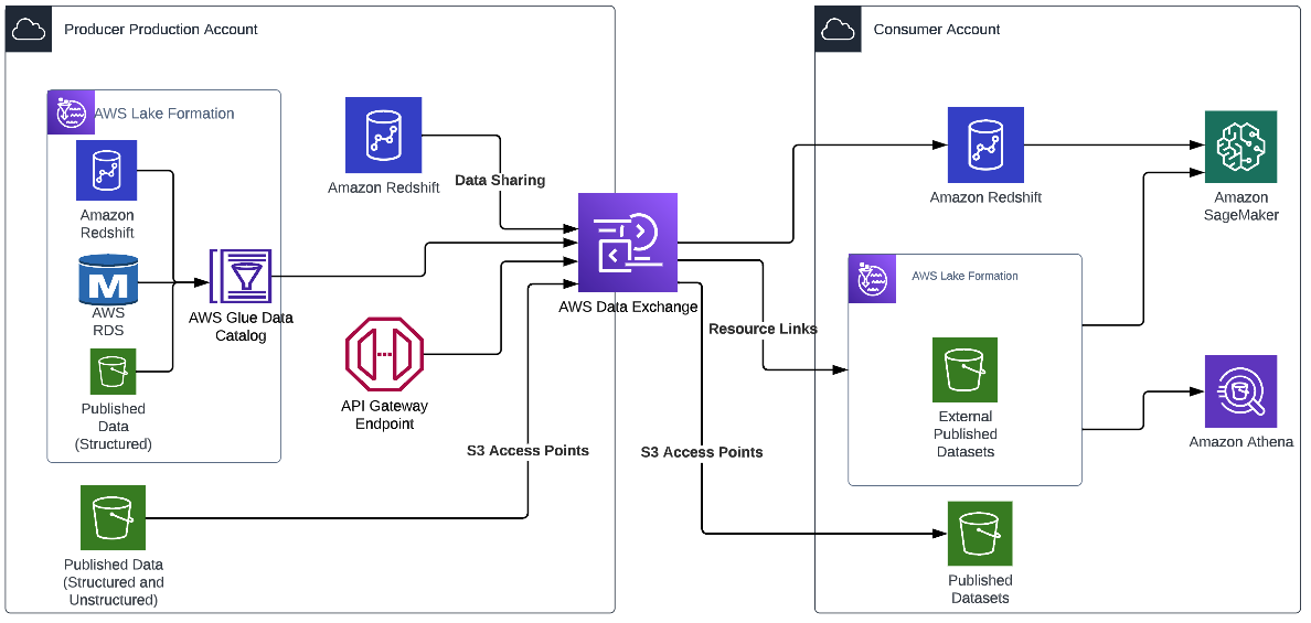
With AWS Data Exchange, once the dataset to share (or sell) is configured, AWS Data Exchange automatically manages entitlements (and billing) between the producer and the consumer. The producer doesn’t have to manage policies, set up new access points, or create new Amazon Redshift data shares for each consumer, and access is automatically revoked if the subscription ends. This can significantly reduce the operational overhead in sharing data.
Pattern 2: Using AWS Lake Formation for centralized access management
You can use this pattern in cases where both the producer and consumer are on the AWS Services with an AWS account that is enabled to use AWS Lake Formation. This pattern provides a no-code approach to data sharing. The following diagram illustrates an example architecture.
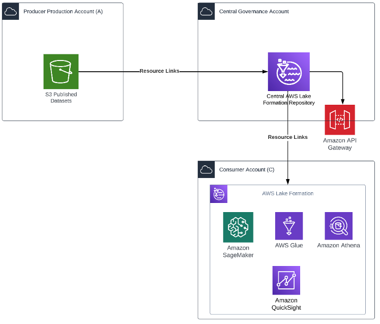
In this pattern, the central governance account has Lake Formation configured for managing access across the producer’s org accounts. Resource links from the production account Amazon Simple Storage Service (Amazon S3) bucket are created in Lake Formation. The producer grants Lake Formation permissions on an AWS Glue Data Catalog resource to an external account, or directly to an AWS Identity and Access Management (IAM) principal in another account. Lake Formation uses AWS Resource Access Manager (AWS RAM) to share the resource. If the grantee account is in the same organization as the grantor account, the shared resource is available immediately to the grantee. If the grantee account is not in the same organization, AWS RAM sends an invitation to the grantee account to accept or reject the resource grant. To make the shared resource available, the consumer administrator in the grantee account must use the AWS RAM console or AWS Command Line Interface (AWS CLI) to accept the invitation.
Authorized principals can share resources explicitly with an IAM principal in an external account. This feature is useful when the producer wants to have control over who in the external account can access the resources. The permissions the IAM principal receives are a union of direct grants and the account-level grants that are cascaded down to the principals. The data lake administrator of the recipient account can view the direct cross-account grants, but can’t revoke permissions.
Pattern 3: Using AWS Lake Formation from the producer external sharing account
The producer may have stringent security requirements where no external consumer should access their production account or their centralized governance account. They may also not have Lake Formation enabled on their production platform. In such cases, as shown in the following diagram, the producer production account (Account A) is dedicated to its internal organization users. The producer creates another account, the producer external sharing account (Account B), which is dedicated for external sharing. This gives the producer more latitude to create specific policies for specific organizations.
The following architecture diagram shows an overview of the pattern.
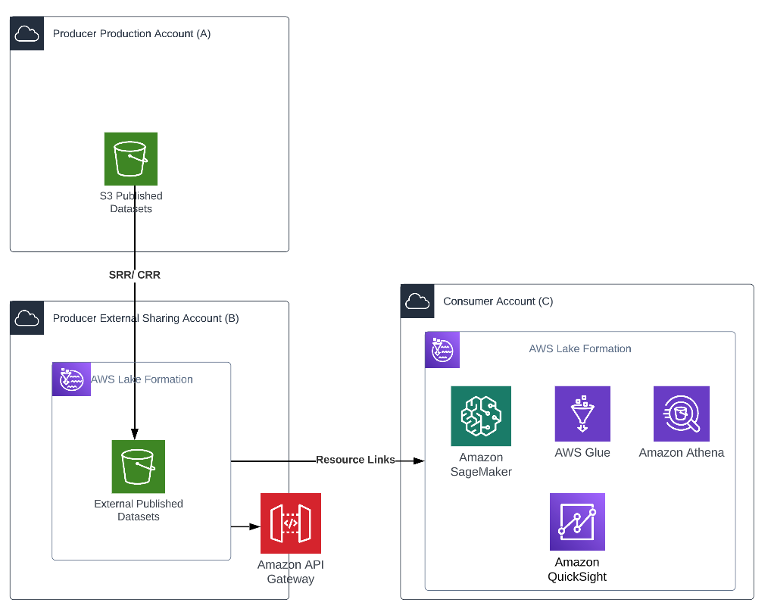
The producer implements a process to create an asynchronous copy of data in Account B. The bucket can be configured for Same Region Replication (SRR) or Cross Region Replication (CRR) for objects that need to be shared. This facilitates automated refresh of data to the external account to the “External Published Datasets” S3 bucket without having to write any code.
Creating a copy of the data allows the producer to add another degree of separation between the external consumer and its production data. It also helps meet any compliance or data sovereignty requirements.
Lake Formation is set up on Account B, and the administrator creates resources links for the “External Published Datasets” S3 bucket in its account to grant access. The administrator follows the same process to grant access as described earlier.
Pattern 4: Using Amazon Redshift data sharing
This pattern is ideally suited for a producer who has most of their published data products on Amazon Redshift. This pattern also requires the producer’s external sharing account (Account B) and the consumer account (Account C) to have an encrypted Amazon Redshift cluster or Amazon Redshift Serverless endpoint that meets the prerequisites for Amazon Redshift data sharing.
The following architecture diagram shows an overview of the pattern.
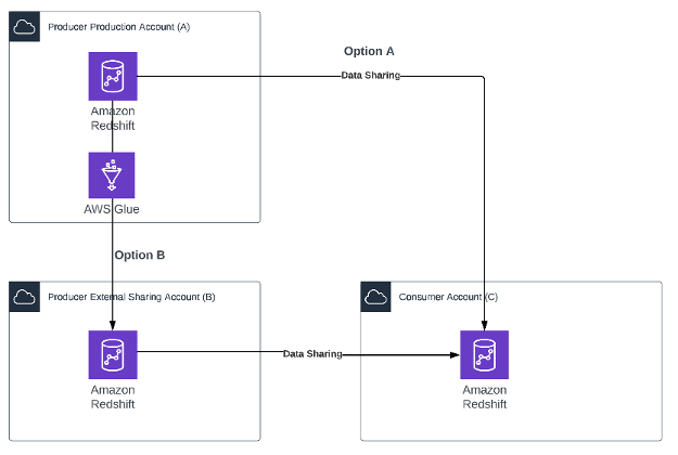
Two options are possible depending on the producer’s compliance constraints:
- Option A – The producer enables data sharing directly on the production Amazon Redshift cluster.
- Option B – The producer may have constraints with respect to sharing the production cluster. The producer creates a simple AWS Glue job that copies data from the Amazon Redshift cluster in the production Account A to the Amazon Redshift cluster in the external Account B. This AWS Glue job can be scheduled to refresh data as needed by the consumer. When the data is available in Account B, the producer can create multiple views and multiple data shares as needed.
In both options, the producer maintains complete control over what data is being shared, and the consumer admin maintains full control over who can access the data within their organization.
After both the producer and consumer admins approve the data sharing request, the consumer user can access this data as if it were part of their own account without have to write any additional code.
Pattern 5: Sharing data securely and privately using APIs
You can adopt this pattern when the external partner doesn’t have a presence on AWS. You can also use this pattern when published data products are spread across various services like Amazon S3, Amazon Redshift, Amazon DynamoDB, and Amazon OpenSearch Service but the producer would like to maintain a single data sharing interface.
Here’s an example use case: Company A would like to share some of its log data in near-real time with its partner Company B, who uses this data to generate predictive insights for Company A. Company A stores this data in Amazon Redshift. The company wants to share this transactional information with its partner after masking the personally identifiable information (PII) in a cost-effective and secure way to generate insights. Company B doesn’t use the AWS Services.
Company A establishes a microbatch process using an AWS Lambda function or AWS Glue that queries Amazon Redshift to get incremental log data, applies the rules to redact the PII, and loads this data to the “Published Datasets” S3 bucket. This instantiates an SRR/CRR process that refreshes this data in the “External Sharing” S3 bucket.
The following diagram shows how the consumer can then use an API-based approach to access this data.
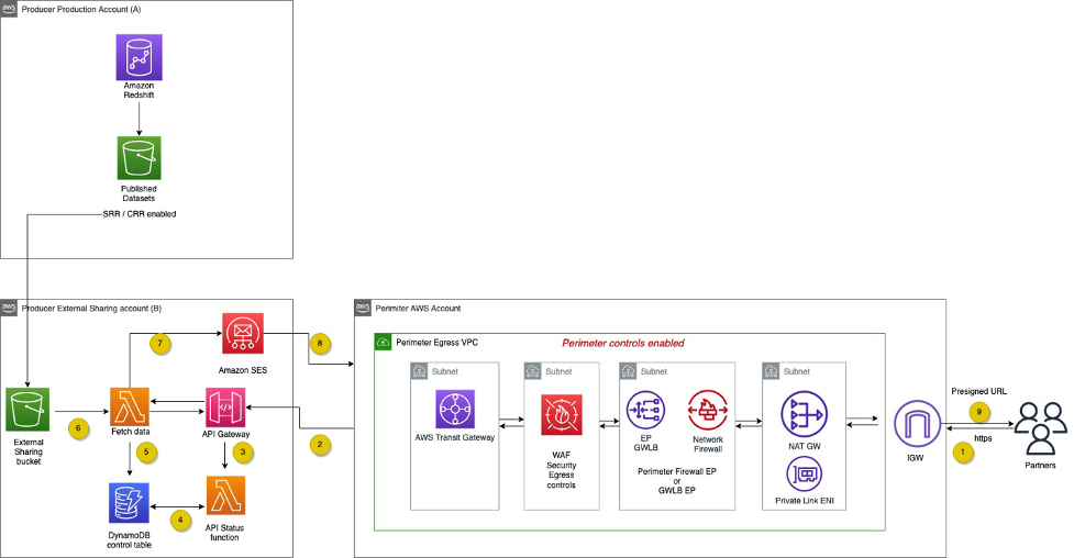
The workflow contains the following steps:
- An HTTPS API request is sent from the API consumer to the API proxy layer.
- The HTTPS API request is forwarded from the API proxy to Amazon API Gateway in the external sharing AWS account.
- Amazon API Gateway calls the request receiver Lambda function.
- The request receiver function writes the status to a DynamoDB control table.
- A second Lambda function, the poller, checks the status of the results in the DynamoDB table.
- The poller function fetches results from Amazon S3.
- The poller function sends a presigned URL to download the file from the S3 bucket to the requestor via Amazon Simple Email Service (Amazon SES).
- The requestor downloads the file using the URL.
- The network perimeter AWS account only allows egress internet connection.
- The API proxy layer enforces both the egress security controls and perimeter firewall before the traffic leaves the producer’s network perimeter.
- The AWS Transit Gateway security egress VPC routing table only allows connectivity from the required producer’s subnet, while preventing internet access.
Pattern 6: Using Amazon S3 access points
Data scientists may need to work collaboratively on image, videos, and text documents. Legal and audit groups may want to share reports and statements with the auditing agencies. This pattern discusses an approach to sharing such documents. The pattern assumes that the external partners are also on AWS. Amazon S3 access points allow the producer to share access with their consumer by setting up cross-account access without having to edit bucket policies.
Access points are named network endpoints that are attached to buckets that you can use to perform S3 object operations, such as GetObject and PutObject. Each access point has distinct permissions and network controls that Amazon S3 applies for any request that is made through that access point. Each access point enforces a customized access point policy that works in conjunction with the bucket policy attached to the underlying bucket.
The following architecture diagram shows an overview of the pattern.
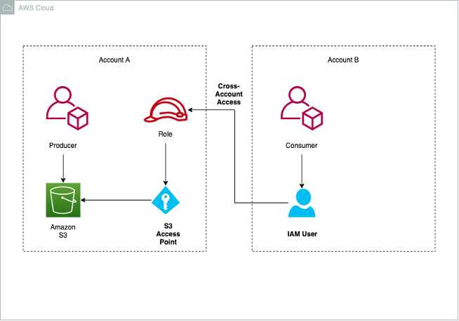
The producer creates an S3 bucket and enables the use of access points. As part of the configuration, the producer specifies the consumer account, IAM role, and privileges for the consumer IAM role.
The consumer users with the IAM role in the consumer account can access the S3 bucket via the internet or restricted to an Amazon VPC via VPC endpoints and AWS PrivateLink.
Conclusion
Each organization has its unique set of constraints and requirements that it needs to fulfill to set up an efficient data sharing solution. In this post, we demonstrated various options and best practices available to organizations. The data platform owner and security team should work together to assess what works best for your specific situation. Your AWS account team is also available to help.
Related resources
For more information on related topics, refer to the following:
- Data perimeters on AWS
- AWS Data Exchange
- Securely share your data across AWS accounts using AWS Lake Formation
- Sharing data across clusters in Amazon Redshift
- Setting up cross-account Amazon S3 access with S3 Access Points
About the Authors
 Venkata Sistla is a Cloud Architect – Data & Analytics at AWS. He specializes in building data processing capabilities and helping customers remove constraints that prevent them from leveraging their data to develop business insights.
 Santosh Chiplunkar is a Principal Resident Architect at AWS. He has over 20 years of experience helping customers solve their data challenges. He helps customers develop their data and analytics strategy and provides them with guidance on how to make it a reality.
Data lakes are a popular choice for today’s organizations to store their data around their business activities. As a best practice of a data lake design, data should be immutable once stored. But regulations such as the General Data Protection Regulation (GDPR) have created obligations for data operators who must be able to erase or update personal data from their data lake when requested.
A data lake built on AWS uses Amazon Simple Storage Service (Amazon S3) as its primary storage environment. When a customer asks to erase or update private data, the data lake operator needs to find the required objects in Amazon S3 that contain the required data and take steps to erase or update that data. This activity can be a complex process for the following reasons:
- Data lakes may contain many S3 objects (each may contain multiple rows), and often it’s difficult to find the object containing the exact data that needs to be erased or personally identifiable information (PII) to be updated as per the request
- By nature, S3 objects are immutable and therefore applying direct row-based transactions like DELETE or UPDATE isn’t possible
To handle these situations, a transactional feature on S3 objects is required, and frameworks such as Apache Hudi or Apache Iceberg provide you the transactional feature for upserts in Amazon S3.
AWS contributed the Apache Iceberg integration with the AWS Glue Data Catalog, which enables you to use open-source data computation engines like Apache Spark with Iceberg on AWS Glue. In 2022, Amazon Athena announced support of Iceberg, enabling transaction queries on S3 objects.
In this post, we show you how to stream real-time data to an Iceberg table in Amazon S3 using AWS Glue streaming and perform transactions using Amazon Athena for deletes and updates. We use a serverless mechanism for this implementation, which requires minimum operational overhead to manage and fine-tune various configuration parameters, and enables you to extend your use case to ACID operations beyond the GDPR.
Solution overview
We used the Amazon Kinesis Data Generator (KDG) to produce synthetic streaming data in Amazon Kinesis Data Streams and then processed the streaming input data using AWS Glue streaming to store the data in Amazon S3 in Iceberg table format. As part of the customer’s request, we ran delete and update statements using Athena with Iceberg support.
The following diagram illustrates the solution architecture.
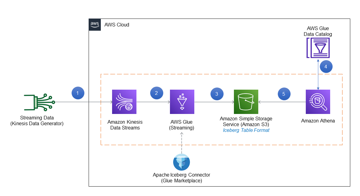
The solution workflow consists of the following steps:
- Streaming data is generated in JSON format using the KDG template and inserted into Kinesis Data Streams.
- An AWS Glue streaming job is connected to Kinesis Data Streams to process the data using the Iceberg connector.
- The streaming job output is stored in Amazon S3 in Iceberg table format.
- Athena uses the AWS Glue Data Catalog to store and retrieve table metadata for the Amazon S3 data in Iceberg format.
- Athena interacts with the Data Catalog tables in Iceberg format for transactional queries required for GDPR.
The codebase required for this post is available in the GitHub repository.
Prerequisites
Before starting the implementation, make sure the following prerequisites are met:
- You have an AWS account
- The Region used for this post is
us-east-1 - You have access to the AWS CloudFormation template from GitHub to set up the basic services and AWS Identity and Access Management (IAM) role
Deploy resources using AWS CloudFormation
Complete the following steps to deploy your solution resources:
- After you sign in to your AWS account, launch the CloudFormation template by choosing Launch Stack:

- For Stack name, enter a name.
- For Username, enter the user name for the KDG.
- For Password, enter the password for the KDG (this must be at least six alphanumeric characters, and contain at least one number).
- For IAMGlueStreamingJobRoleName, enter a name for the IAM role used for the AWS Glue streaming job.
- Choose Next and create your stack.

This CloudFormation template configures the following resources in your account:
- An S3 bucket named
streamingicebergdemo-XX(note that the XX part is a random unique number to make the S3 bucket name unique) - An IAM policy and role
- The KDG URL used for creating synthetic data
- After you complete the setup, go to the Outputs tab of the CloudFormation stack to get the S3 bucket name, AWS Glue job execution role (as per your input), and KDG URL.

- Before proceeding with the demo, create a folder named
custdataunder the created S3 bucket.

Create a Kinesis data stream
We use Kinesis Data Streams to create a serverless streaming data service that is built to handle millions of events with low latency. The following steps guide you on how to create the data stream in the us-east-1 Region:
- Log in to the AWS Management Console.
- Navigate to Kinesis console (make sure the Region is
us-east-1). - Select Kinesis Data Streams and choose Create data stream.

- For Data stream name, enter
demo-data-stream. - For this post, we select On-demand as the Kinesis data stream capacity mode.
On-demand mode works to eliminate the need for provisioning and managing the capacity for streaming data. However, you can implement this solution with Kinesis Data Streams in provisioned mode as well.
- Choose Create data stream.

- Wait for successful creation of
demo-data-streamand for it to be inActivestatus.

Set up the Kinesis Data Generator
To create a sample streaming dataset, we use the KDG URL generated on the CloudFormation stack Outputs tab and log in with the credentials used in the parameters for the CloudFormation template. For this post, we use the following template to generate sample data in the demo-data-stream Kinesis data stream.
- Log in to the KDG URL with the user name and password you supplied during stack creation.
- Change the Region to
us-east-1. - Select the Kinesis data stream
demo-data-stream. - For Records per second, choose Constant and enter
100(it can be another number, depending on the rate of record creation). - On the Template 1 tab, enter the KDG data generation template:
- Choose Test template to test the sample records.
- When the testing is correct, choose Send data.
This will start sending 100 records per second in the Kinesis data stream. (To stop sending data, choose Stop Sending Data to Kinesis.)
Integrate Iceberg with AWS Glue
To add the Apache Iceberg Connector for AWS Glue, complete the following steps. The connector is free to use and supports AWS Glue 1.0, 2.0, and 3.0.
- On the AWS Glue console, choose AWS Glue Studio in the navigation pane.
- In the navigation pane, navigate to AWS Marketplace.
- Search for and choose Apache Iceberg Connector for AWS Glue.

- Choose Accept Terms and Continue to Subscribe.

- Choose Continue to Configuration.
- For Fulfillment option, choose your AWS Glue version.
- For Software version, choose the latest software version.
- Choose Continue to Launch.

- Under Usage Instructions, choose the link to activate the connector.

- Enter a name for the connection, then choose Create connection and activate the connector.

- Verify the new connector on the AWS Glue Studio Connectors.

Create the AWS Glue Data Catalog database
The AWS Glue Data Catalog contains references to data that is used as sources and targets of your extract, transform, and load (ETL) jobs in AWS Glue. To create your data warehouse or data lake, you must catalog this data. The AWS Glue Data Catalog is an index to the location and schema of your data. You use the information in the Data Catalog to create and monitor your ETL jobs.
For this post, we create a Data Catalog database named icebergdemodb containing the metadata information of a table named customer, which will be queried through Athena.
- On the AWS Glue console, choose Databases in the navigation pane.
- Choose Add database.
- For Database name, enter
icebergdemodb.
This creates an AWS Glue database for metadata storage.
Create a Data Catalog table in Iceberg format
In this step, we create a Data Catalog table in Iceberg table format.
- On the Athena console, create an Athena workgroup named
demoworkgroupfor SQL queries. - Choose Athena engine version 3 for Query engine version.
For more information about Athena versions, refer to Changing Athena engine versions.

- Enter the S3 bucket location for Query result configuration under Additional configurations.

- Open the Athena query editor and choose
demoworkgroup. - Choose the database
icebergdemodb. - Enter and run the following DDL to create a table pointing to the Data Catalog database
icerbergdemodb. Note that theTBLPROPERTIESsection mentionsICEBERGas the table type andLOCATIONpoints to the S3 folder (custdata) URI created in earlier steps. This DDL command is available on the GitHub repo.

After you run the command successfully, you can see the table customer in the Data Catalog.

Create an AWS Glue streaming job
In this section, we create the AWS Glue streaming job, which fetches the record from the Kinesis data stream using the Spark script editor.
- On the AWS Glue console, choose Jobs (new) in the navigation pane.

- For Create job¸ select Spark script editor.
- For Options¸ select Create a new script with boilerplate code.
- Choose Create.

- Enter the code available in the GitHub repo in the editor.
The sample code keeps appending data in the target location by fetching records from the Kinesis data stream.
- Choose the Job details tab in the query editor.
- For Name, enter
Demo\_Job. - For IAM role¸ choose
demojobrole. - For Type, choose Spark Streaming.
- For Glue Version, choose Glue 3.0.
- For Language, choose Python 3.
- For Worker type, choose G 0.25X.
- Select Automatically scale the number of workers.
- For Maximum number of workers, enter
5.

- Under Advanced properties, select Use Glue Data Catalog as the Hive metastore.
- For Connections, choose the connector you created.
- For Job parameters, enter the following key pairs (provide your S3 bucket and account ID):
| Key | Value |
--iceberg\_job\_catalog\_warehouse | s3://streamingicebergdemo-XX/custdata/ |
--output\_path | s3://streamingicebergdemo-XX |
--kinesis\_arn | arn:aws:kinesis:us-east-1:<AWS Account ID>:stream/demo-data-stream |
--user-jars-first | True |

- Choose Run to start the AWS Glue streaming job.
- To monitor the job, choose Monitoring in the navigation pane.
- Select
Demo\_Joband choose View run details to check the job run details and Amazon CloudWatch logs.

Run GDPR use cases on Athena
In this section, we demonstrate a few use cases that are relevant to GDPR alignment with the user data that’s stored in Iceberg format in the Amazon S3-based data lake as implemented in the previous steps. For this, let’s consider that the following requests are being initiated in the workflow to comply with the regulations:
- Delete the records for the input
customerid(for example,59289) - Update
phonenumberfor thecustomerid(for example,51936)
The IDs used in this example are samples only because they were created through the KDG template used earlier, which creates sample data. You can search for IDs in your implementation by querying through the Athena query editor. The steps remain the same.
Delete data by customer ID
Complete the following steps to fulfill the first use case:
- On the Athena console, and make sure
icebergdemodbis chosen as the database. - Open the query editor.
- Enter the following query using a customer ID and choose Run:
This query gives the count of records for the input customerid before delete.

- Enter the following query with the same customer ID and choose Run:
This query deletes the data for the input customerid as per the workflow generated.

- Test if there is data with the customer ID using a count query.
The count should be 0.

Update data by customer ID
Complete the following steps to test the second use case:
- On the Athena console, make sure
icebergdemodbis chosen as the database. - Open the query editor.
- Enter the following query with a customer ID and choose Run.
This query gives the value for phonenumber before update.

- Run the following query to update the required columns:
This query updates the data to a dummy value.

- Run the SELECT query to check the update.
You can see the data is updated correctly.

Vacuum table
A good practice is to run the VACUUM command periodically on the table because operations like INSERT, UPDATE, DELETE, and MERGE will take place on the Iceberg table. See the following code:

Considerations
The following are a few considerations to keep in mind for this implementation:
- Review the considerations and limitations for Athena support for Iceberg table format. For example, Athena only creates and operates on Iceberg v2 tables. To learn more about AWS integrations, refer to Iceberg AWS integrations.
- Check the AWS Glue streaming ETL notes and restrictions for AWS Glue streaming jobs.
Clean up
Complete the following steps to clean up the resources you created for this post:
-
- Delete the custdata folder in the S3 bucket.
- Delete the CloudFormation stack.
- Delete the Kinesis data stream.
- Delete the S3 bucket storing the data.
- Delete the AWS Glue job and Iceberg connector.
- Delete the AWS Glue Data Catalog database and table.
- Delete the Athena workgroup.
- Delete the IAM roles and policies.
Conclusion
This post explained how you can use the Iceberg table format on Athena to implement GDPR use cases like data deletion and data upserts as required, when streaming data is being generated and ingested through AWS Glue streaming jobs in Amazon S3.
The operations for the Iceberg table that we demonstrated in this post aren’t all of the data operations that Iceberg supports. Refer to the Apache Iceberg documentation for details on various operations.
About the Authors
 Dhiraj Thakur is a Solutions Architect with Amazon Web Services. He works with AWS customers and partners to provide guidance on enterprise cloud adoption, migration, and strategy. He is passionate about technology and enjoys building and experimenting in the analytics and AI/ML space.
 Rajdip Chaudhuri is Solutions Architect with Amazon Web Services specializing in data and analytics. He enjoys working with AWS customers and partners on data and analytics requirements. In his spare time, he enjoys soccer.
Data lakes provide a centralized repository that consolidates your data at scale and makes it available for different kinds of analytics. AWS Glue crawlers are a popular way to scan data in a data lake, classify it, extract schema information from it, and store the metadata automatically in the AWS Glue Data Catalog. AWS Lake Formation enables you to centrally govern, secure, and share your data, and lets you scale permissions easily.
We are pleased to announce AWS Glue crawler and Lake Formation integration. You can now use Lake Formation permissions for the crawler’s access to your Lake Formation managed data lakes, whether those are in your account or in other accounts. Before this release, you had to set up AWS Glue crawler IAM role with Amazon Simple Storage Service (Amazon S3) permissions to crawl data source on Amazon S3. And also establish Amazon S3 bucket policies on the source bucket for the crawler role to access S3 data source. Now you can use AWS Lake Formation permission defined on data lake for crawling the data and you no longer need to configure dedicated Amazon S3 permissions for crawlers. AWS Lake Formation manages crawler IAM role access to various Amazon S3 buckets and/or its prefix using data locations permissions to simplify security management. Further you can apply the same security model for crawlers in addition to AWS Glue jobs, Amazon Athena for centralized governance.
When you configure an AWS Glue crawler to use Lake Formation, by default, the crawler uses Lake Formation in the same account to obtain data access credentials. However, you can also configure the crawler to use Lake Formation of a different account by providing an account ID during creation. The cross-account capability allows you to perform permissions management from a central governance account. Customers prefer the central governance experience over writing bucket policies separately in each bucket-owning account. To build a data mesh architecture, you can author permissions in a single Lake Formation governance to manage access to data locations and crawlers spanning multiple accounts in your data lake. You can refer to How to configure a crawler to use Lake Formation credentials for more information.
In this post, we walk through a single in-account architecture that shows how to enable Lake Formation permissions on the data lake, configure an AWS Glue crawler with Lake Formation permission to scan and populate schema from an S3 data lake into the AWS Glue Data Catalog, and then use an analytical engine like Amazon Athena to query the data.
Solution overview
The AWS Glue crawler and Lake Formation integration supports in-account crawling as well as cross-account crawling. You can configure a crawler to use Lake Formation permissions to access an S3 data store or a Data Catalog table with an underlying S3 location within the same AWS account or another AWS account. You can configure an existing Data Catalog table as a crawler’s target if the crawler and the Data Catalog table reside in the same account. The following figure shows the in-account crawling architecture.

Prerequisites
Complete the following prerequisite steps:
- Sign in to the Lake Formation console as admin.
- If this is the first time accessing the Lake Formation console, add yourself as the data lake administrator.

- In the navigation pane, under Data catalog, choose Settings.
- Deselect Use only IAM access control for new databases.
- Deselect Use only IAM access control for new tables in new databases.
- Keep Version 3 as the current cross-account version.
- Choose Save.
Set up your solution resources
We set up the solution resources using AWS CloudFormation. Complete the following steps:
- Log in to the AWS Management Console as IAM administrator.
- Choose Launch Stack to deploy a CloudFormation template:
- For LFBusinessAnalystUserName, keep as the default
LFBusinessAnalyst. - Create your stack.
- When the stack is complete, on the AWS CloudFormation console, navigate to the Resources tab of the stack.
- Note down value of
Databasename,DataLakeBucket, andGlueCrawlerName. - Choose the
LFBusinessAnalystUserCredentialsvalue to navigate to the AWS Secrets Manager console.

- In the Secret value section, choose Retrieve secret value.
- Note down the secret value for the password for IAM user
LFBusinessAnalyst.
Validate resources
In your account, validate the following resources created by template:
- AWS Glue database – The Databasename value noted from the CloudFormation template.
- S3 bucket for the data lake with sample data – The
DataLakeBucketvaluevalue noted from the CloudFormation template. - AWS Glue crawler and IAM role with required permission – The
GlueCrawlerNamevalue noted from the CloudFormation template.
The template registers the S3 bucket with Lake Formation as the data location. On Lake Formation console left navigation choose Data lake locations under Register and ingest.

The template also grants data location permission on the S3 bucket to the crawler role. On Lake Formation console left navigation choose Data locations under Permissions.

Lastly, the template grants database permission to the crawler role. On Lake Formation console left navigation choose Data lake permissions under Permissions.

Edit and run the AWS Glue crawler
To configure and run the AWS Glue crawler, complete the following steps:
- On the AWS Glue console, choose Crawlers in the navigation pane.
- Locate the crawler
lfcrawler-<your-account-id>and edit it. - Under Lake Formation configuration, select Use Lake Formation credentials for crawling S3 data source.
- Choose Next.

- Review and update the crawler settings.
Note that the crawler IAM role uses Lake Formation permission to access the data and doesn’t have any S3 policies.

- Run the crawler and verify that the crawler run is complete.

- In the AWS Glue database
lfcrawlerdb<your-account-id>, verify that the table is created and the schema matches with what you have in the S3 bucket.

The crawler was able to crawl the S3 data source and successfully populate the schema using Lake Formation permissions.
Grant access to the data analyst using Lake Formation
Now the data lake admin can delegate permissions on the database and table to the LFBusinessAnalyst user via the Lake Formation console.
Grant the LFBusinessAnalyst IAM user access to the database with Describe permissions.
- On the Lake Formation console, under Permissions in the navigation pane, choose Data lake permission .
- Choose Grant
- Under Principals, select IAM users and roles.
- Choose the IAM users
LFBusinessAnalyst - Under LF-Tags or catalog resources, choose
lfcrawlerdb<your-accountid>for Databases. - Select Describe for Database permissions.
- Choose Grant to apply the permissions.

Grant the LFBusinessAnalyst IAM user Select and Describe access to the table.
- On the Lake Formation console, under Permissions in the navigation pane, choose Data lake permission.
- Choose Grant.
- Under Principals, select IAM users and roles.
- Choose the IAM users
LFBusinessAnalyst. - Under LF-Tags or catalog resources, choose
lfcrawlerdb<your-accountid>for Databases andlf\_datalake\_<your-accountid>\_<region>for Tables - Choose Select, Describe for Table permissions.
- Choose Grant to apply the permissions.

Verify the tables using Athena
To verify the tables using Athena, complete the following steps:
- Log in as
LFBusinessAnalystusing the password noted earlier through the CloudFormation stack. - On the Athena console, choose
lfconsumer-primary-workgroupas the Athena workgroup. - Run the query to validate access as shown in the following screenshot.

We have successfully crawled Amazon S3 data store using the crawler with Lake Formation permission and populated the metadata in AWS Glue Data Catalog. We have granted Lake Formation permission on database and table to consumer user and validated user access to the data using Athena.
Clean up
To avoid unwanted charges to your AWS account, you can delete the AWS resources:
- Sign in to the CloudFormation console as the IAM admin used for creating the CloudFormation stack.
- Delete the stack you created.
Summary
In this post, we showed how to use the new AWS Glue crawler integration with Lake Formation. Data lake admins can now share crawled tables with data analysts using Lake Formation, allowing analysts to use analytical services such as Athena. You can centrally manage all permissions in Lake Formation, making it easier to administer and protect data lakes.
Special thanks to everyone who contributed to this crawler feature launch: Anshuman Sharma, Jessica Cheng, Aditya K, Sandya Krishnanand
If you have questions or suggestions, submit them in the comments section.
About the authors
Sandeep Adwankar is a Senior Technical Product Manager at AWS. Based in the California Bay Area, he works with customers around the globe to translate business and technical requirements into products that enable customers to improve how they manage, secure, and access data.
Srividya Parthasarathy is a Senior Big Data Architect on the AWS Lake Formation team. She enjoys building data mesh solutions and sharing them with the community.
Amazon QuickSight Enterprise edition can integrate with your existing Microsoft Active Directory (AD), providing federated access using Security Assertion Markup Language (SAML) to dashboards. Using existing identities from Active Directory eliminates the need to create and manage separate user identities in AWS Identity Access Management (IAM). Federated users assume an IAM role when access is requested through an identity provider (IdP) such as Active Directory Federation Service (AD FS) based on AD group membership. Although, you can connect AD to QuickSight using AWS Directory Service, this blog focuses on federated logon to QuickSight Dashboards.
With identity federation, your users get one-click access to Amazon QuickSight applications using their existing identity credentials. You also have the security benefit of identity authentication by your IdP. You can control which users have access to QuickSight using your existing IdP. Refer to Using identity federation and single sign-on (SSO) with Amazon QuickSight for more information.
In this post, we demonstrate how you can use a corporate email address as an authentication option for signing in to QuickSight. This post assumes you have an existing Microsoft Active Directory Federation Services (ADFS) configured in your environment.
Solution overview
While connecting to QuickSight from an IdP, your users initiate the sign-in process from the IdP portal. After the users are authenticated, they are automatically signed in to QuickSight. After QuickSight checks that they are authorized, your users can access QuickSight.
The following diagram shows an authentication flow between QuickSight and a third-party IdP. In this example, the administrator has set up a sign-in page to access QuickSight. When a user signs in, the sign-in page posts a request to a federation service that complies with SAML 2.0. The end-user initiates authentication from the sign-in page of the IdP. For more information about the authentication flow, see Initiating sign-on from the identity provider (IdP).

The solution consists of the following high-level steps:
- Create an identity provider.
- Create IAM policies.
- Create IAM roles.
- Configure AD groups and users.
- Create a relying party trust.
- Configure claim rules.
- Configure QuickSight single sign-on (SSO).
- Configure the relay state URL for QuickStart.
Prerequisites
The following are the prerequisites to build the solution explained in this post:
- An existing or newly deployed AD FS environment.
- An AD user with permissions to manage AD FS and AD group membership.
- An IAM user with permissions to create IAM policies and roles, and administer QuickSight.
- The metadata document from your IdP. To download it, refer to Federation Metadata Explorer.
Create an identity provider
To add your IdP, complete the following steps:
- On the IAM console, choose Identity providers in the navigation pane.
- Choose Add provider.
- For Provider type¸ select SAML.
- For Provider name, enter a name (for example,
QuickSight\_Federation). - For Metadata document, upload the metadata document you downloaded as a prerequisite.
- Choose Add provider.
- Copy the ARN of this provider to use in a later step.

Create IAM policies
In this step, you create IAM policies that allow users to access QuickSight only after federating their identities. To provide access to QuickSight and also the ability to create QuickSight admins, authors (standard users), and readers, use the following policy examples.
The following code is the author policy:
The following code is the reader policy:
The following code is the admin policy:
Create IAM roles
You can configure email addresses for your users to use when provisioning through your IdP to QuickSight. To do this, add the sts:TagSession action to the trust relationship for the IAM role that you use with AssumeRoleWithSAML. Make sure the IAM role names start with ADFS-.
- On the IAM console, choose Roles in the navigation pane.
- Choose Create new role.
- For Trusted entity type, select SAML 2.0 federation.
- Choose the SAML IdP you created earlier.
- Select Allow programmatic and AWS Management Console access.
- Choose Next.

- Choose the admin policy you created, then choose Next.
- For Name, enter
ADFS-ACCOUNTID-QSAdmin. - Choose Create.
- On the Trust relationships tab, edit the trust relationships as follows so you can pass principal tags when users assume the role (provide your account ID and IdP):
- Repeat this process for the role
ADFS-ACCOUNTID-QSAuthorand attach the author IAM policy. - Repeat this process for the role
ADFS-ACCOUNTID-QSReaderand attach the reader IAM policy.
Configure AD groups and users
Now you need to create AD groups that determine the permissions to sign in to AWS. Create an AD security group for each of the three roles you created earlier. Note that the group name should follow same format as your IAM role names.
One approach for creating the AD groups that uniquely identify the IAM role mapping is by selecting a common group naming convention. For example, your AD groups would start with an identifier, for example AWS-, which will distinguish your AWS groups from others within the organization. Next, include the 12-digit AWS account number. Finally, add the matching role name within the AWS account. You should do this for each role and corresponding AWS account you wish to support with federated access. The following screenshot shows an example of the naming convention we use in this post.

Later in this post, we create a rule to pick up AD groups starting with AWS-, the rule will remove AWS-ACCOUNTID- from AD groups name to match the respective IAM role, which is why we use this naming convention here.
Users in Active Directory can subsequently be added to the groups, providing the ability to assume access to the corresponding roles in AWS. You can add AD users to the respective groups based on your business permissions model. Note that each user must have an email address configured in Active Directory.
Create a relying party trust
To add a relying party trust, complete the following steps:
- Open the AD FS Management Console.
- Choose (right-click) Relying Party Trusts, then choose Add Relying Party Trust.

- Choose Claims aware, then choose Start.
- Select Import data about the relying party published online or on a local network.
- For Federation metadata address, enter
https://signin.aws.amazon.com/static/saml-metadata.xml. - Choose Next.

- Enter a descriptive display name, for example Amazon QuickSight Federation, then choose Next.
- Choose your access control policy (for this post, Permit everyone), then choose Next.

- In the Ready to Add Trust section, choose Next.

- Leave the defaults, then choose Close.
Configure claim rules
In this section, you create claim rules that identify accounts, set LDAP attributes, get the AD groups, and match them to the roles created earlier. Complete the following steps to create the claim rules for NameId, RoleSessionName, Get AD Groups, Roles, and (optionally) Session Duration:
- Select the relying party trust you just created, then choose Edit Claim Issuance Policy.
- Add a rule called
NameIdwith the following parameters:- For Claim rule template, choose Transform an Incoming Claim.
- For Claim rule name, enter NameId
- For Incoming claim type, choose Windows account name.
- For Outgoing claim type, choose Name ID.
- For Outgoing name ID format, choose Persistent Identifier.
- Select Pass through all claim values.
- Choose Finish.

- Add a rule called
RoleSessionNamewith the following parameters:- For Claim rule template, choose Send LDAP Attributes as Claims.
- For Claim rule name, enter
RoleSessionName. - For Attribute store, choose Active Directory.
- For LDAP Attribute, choose E-Mail-Addresses.
- For Outgoing claim type, enter
https://aws.amazon.com/SAML/Attributes/RoleSessionName. - Add another E-Mail-Addresses LDAP attribute and for Outgoing claim type, enter
https://aws.amazon.com/SAML/Attributes/PrincipalTag:Email. - Choose OK.

- Add a rule called
Get AD Groupswith the following parameters:- For Claim rule template, choose Send Claims Using a Custom Rule.
- For Claim rule name, enter Get AD Groups
- For Custom Rule, enter the following code:
- Choose OK.

- Add a rule called
Roleswith the following parameters:- For Claim rule template, choose Send Claims Using a Custom Rule.
- For Claim rule name, enter Roles
- For Custom Rule, enter the following code (provide your account ID and IdP):
- Choose Finish.

Optionally, you can create a rule called Session Duration. This configuration determines how long a session is open and active before users are required to reauthenticate. The value is in seconds. For this post, we configure the rule for 8 hours.
- Add a rule called
Session Durationwith the following parameters:- For Claim rule template, choose Send Claims Using a Custom Rule.
- For Claim rule name, enter
Session Duration. - For Custom Rule, enter the following code:
- Choose Finish.

You should be able to see these five claim rules, as shown in the following screenshot.

- Choose OK.
- Run the following commands in PowerShell on your AD FS server:
- Stop and start the AD FS service from PowerShell:
Configure E-mail Syncing
With QuickSight Enterprise edition integrated with an IdP, you can restrict new users from using personal email addresses. This means users can only log in to QuickSight with their on-premises configured email addresses. This approach allows users to bypass manually entering an email address. It also ensures that users can’t use an email address that might differ from the email address configured in Active Directory.
QuickSight uses the preconfigured email addresses passed through the IdP when provisioning new users to your account. For example, you can make it so that only corporate-assigned email addresses are used when users are provisioned to your QuickSight account through your IdP. When you configure email syncing for federated users in QuickSight, users who log in to your QuickSight account for the first time have preassigned email addresses. These are used to register their accounts.
To configure E-mail syncing for federated users in QuickSight, complete the following steps:
- Log in to your QuickSight dashboard with a QuickSight administrator account.
- Choose the profile icon.

- On the drop-down menu, choose on Manage QuickSight.
- In the navigation pane, choose Single sign-on (SSO).
- For Email Syncing for Federated Users, select ON, then choose Enable in the pop-up window.
- Choose Save.

Configure the relay state URL for QuickStart
To configure the relay state URL, complete the following steps (revise the input information as needed to match your environment’s configuration):
- Use the ADFS RelayState Generator to generate your URL.
- For IDP URL String, enter
https://ADFSServerEndpoint/adfs/ls/idpinitiatedsignon.aspx. - For Relying Party Identifier, enter
urn:amazon:webservicesorhttps://signin.aws.amazon.com/saml. - For Relay State/Target App, enter your authenticated users to access. In this case, it’s
https://quicksight.aws.amazon.com. - Choose Generate URL.

- Copy the URL and load it in your browser.
You should be presented with a login to your IdP landing page.

Make sure the user logging in has an email address attribute configured in Active Directory. A successful login should redirect you to the QuickSight dashboard after authentication. If you’re not redirected to the QuickSight dashboard page, make sure you ran the commands listed earlier after you configured your claim rules.
Summary
In this post, we demonstrated how to configure federated identities to a QuickSight dashboard and ensure that users can only sign in with preconfigured email address in your existing Active Directory.
We’d love to hear from you. Let us know what you think in the comments section.
About the Author
 Adeleke Coker is a Global Solutions Architect with AWS. He helps customers globally accelerate workload deployments and migrations at scale to AWS. In his spare time, he enjoys learning, reading, gaming and watching sport events.
This is a guest post co-written with Raghu Boppanna from Vanguard.
At Vanguard, the Enterprise Advice line of business improves investor outcomes through digital access to superior, personalized, and affordable financial advice. They made it possible, in part, by driving economies of scale across the globe for investors with a highly resilient and efficient technical platform. Vanguard opted for a multi-Region architecture for this workload to help protect against impairments of Regional services. For high availability purposes, there is a need to make the data used by the workload available not just in the primary Region, but also in the secondary Region with minimal replication lag. In the event of a service impairment in the primary Region, the solution should be able to fail over to the secondary Region with as little data loss as possible and the ability to resume data ingestion.
Vanguard Cloud Technology Office and AWS partnered to build an infrastructure solution on AWS that met their resilience requirements. The multi-Region solution enables a robust fail-over mechanism, with built-in observability and recovery. The solution also supports streaming data from multiple sources to different Kinesis data streams. The solution is currently being rolled out to the different lines of business teams to improve the resilience posture of their workloads.
The use case discussed here requires Change Data Capture (CDC) to stream data from a remote data source (mainframe DB2) to Amazon Kinesis Data Streams, because the business capability depends on this data. Kinesis Data Streams is a fully managed, massively scalable, durable, and low-cost streaming service that can continuously capture and stream large amounts of data from multiple sources, and makes the data available for consumption within milliseconds. The service is built to be highly resilient and uses multiple Availability Zones to process and store data.
The solution discussed in this post explains how AWS and Vanguard innovated to build a resilient architecture to meet their high availability goals.
Solution overview
The solution uses AWS Lambda to replicate data from Kinesis data streams in the primary Region to a secondary Region. In the event of any service impairment impacting the CDC pipeline, the failover process promotes the secondary Region to primary for the producers and consumers. We use Amazon DynamoDB global tables for replication checkpoints that allows to resume data streaming from the checkpoint and also maintains a primary Region configuration flag that prevents an infinite replication loop of the same data back and forth.
The solution also provides the flexibility for Kinesis Data Streams consumers to use the primary or any secondary Region within the same AWS account.
The following diagram illustrates the reference architecture.

Let’s look at each component in detail:
- CDC processor (producer) – In this reference architecture, the producer is deployed on Amazon Elastic Compute Cloud (Amazon EC2) in both the primary and secondary Regions, and is active in the primary Region and on standby mode in the secondary Region. It captures CDC data from the external data source (like a DB2 database as shown in the architecture above), and streams to Kinesis Data Streams in the primary Region. Vanguard uses a 3rd party tool Qlik Replicate as their CDC Processor. It produces a well-formed payload including the DB2 commit timestamp to the Kinesis data stream, in addition to the actual row data from the remote data source. (
example-stream-1in this example). The following code is a sample payload containing only the primary key of the record that changed and the commit timestamp (for simplicity, the rest of the table row data is not shown below):{ "eventSource": "aws:kinesis", "kinesis": { "ApproximateArrivalTimestamp": "Mon July 18 20:00:00 UTC 2022", "SequenceNumber": "49544985256907370027570885864065577703022652638596431874", "PartitionKey": "12349999", "KinesisSchemaVersion": "1.0", "Data": "eyJLZXkiOiAxMjM0OTk5OSwiQ29tbWl0VGltZXN0YW1wIjogIjIwMjItMDctMThUMjA6MDA6MDAifQ==" }, "eventId": "shardId-000000000000:49629136582982516722891309362785181370337771525377097730", "invokeIdentityArn": "arn:aws:iam::6243876582:role/kds-crr-LambdaRole-1GZWP67437SD", "eventName": "aws:kinesis:record", "eventVersion": "1.0", "eventSourceARN": "arn:aws:kinesis:us-east-1:6243876582:stream/kds-stream-1/consumer/kds-crr:6243876582", "awsRegion": "us-east-1"}The Base64 decoded value of
Datais as follows. The actual Kinesis record would contain the entire row data of the table row that changed, in addition to the primary key and the commit timestamp.{"Key": 12349999,"CommitTimestamp": "2022-07-18T20:00:00"}The
CommitTimestampin theDatafield is used in the replication checkpoint and is critical to accurately track how much of the stream data has been replicated to the secondary Region. The checkpoint can then be used to facilitate a CDC processor (producer) failover and accurately resume producing data from the replication checkpoint timestamp onwards.The alternative to using a remote data source
CommitTimestamp(if unavailable) is to use theApproximateArrivalTimestamp(which is the timestamp when the record is actually written to the data stream). - Cross-Region replication Lambda function – The function is deployed to both primary and secondary Regions. It’s set up with an event source mapping to the data stream containing CDC data. The same function can be used to replicate data of multiple streams. It’s invoked with a batch of records from Kinesis Data Streams and replicates the batch to a target replication Region (which is provided via the Lambda configuration environment). For cost considerations, if the CDC data is actively produced into the primary Region only, the reserved concurrency of the function in the secondary Region can be set to zero, and modified during regional failover. The function has AWS Identity and Access Management (IAM) role permissions to do the following:
- Read and write to the DynamoDB global tables used in this solution, within the same account.
- Read and write to Kinesis Data Streams in both Regions within the same account.
- Publish custom metrics to Amazon CloudWatch in both Regions within the same account.
- Replication checkpoint – The replication checkpoint uses the DynamoDB global table in both the primary and secondary Regions. It’s used by the cross-Region replication Lambda function to persist the commit timestamp of the last replication record as the replication checkpoint for every stream that is configured for replication. For this post, we create and use a global table called
kdsReplicationCheckpoint. - Active Region config – The active Region uses the DynamoDB global table in both primary and secondary Regions. It uses the native cross-Region replication capability of the global table to replicate the configuration. It’s pre-populated with data about which is the primary Region for a stream, to prevent replication back to the primary Region by the Lambda function in the standby Region. This configuration may not be required if the Lambda function in the standby Region has a reserved concurrency set to zero, but can serve as a safety check to avoid infinite replication loop of the data. For this post, we create a global table called
kdsActiveRegionConfigand put an item with the following data:{ "stream-name": "example-stream-1", "active-region" : "us-east-1"} - Kinesis Data Streams – The stream to which the CDC processor produces the data. For this post, we use a stream called
example-stream-1in both the Regions, with the same shard configuration and access policies.
Sequence of steps in cross-Region replication
Let’s briefly look at how the architecture is exercised using the following sequence diagram.

The sequence consists of the following steps:
- The CDC processor (in
us-east-1) reads the CDC data from the remote data source. - The CDC processor (in
us-east-1) streams the CDC data to Kinesis Data Streams (inus-east-1). - The cross-Region replication Lambda function (in us-east-1) consumes the data from the data stream (in
us-east-1). The enhanced fan-out pattern is recommended for dedicated and increased throughput for cross-Region replication. - The replicator Lambda function (in
us-east-1) validates its current Region with the active Region configuration for the stream being consumed, with the help of thekdsActiveRegionConfigDynamoDB global tableThe following sample code (in Java) can help illustrate the condition being evaluated:// Fetch the current AWS Region from the Lambda function’s environmentString currentAWSRegion = System.getenv(“AWS\_REGION”);// Read the stream name from the first Kinesis Record once for the entire batch being processed. This is done because we are reusing the same Lambda function for replicating multiple streams.String currentStreamNameConsumed = kinesisRecord.getEventSourceARN().split(“:”)[5].split(“/”)[1];// Build the DynamoDB query condition using the stream nameMap<String, Condition> keyConditions = singletonMap(“streamName”, Condition.builder().comparisonOperator(EQ).attributeValueList(AttributeValue.builder().s(currentStreamNameConsumed).build()).build());// Query the DynamoDB Global TableQueryResponse queryResponse = ddbClient.query(QueryRequest.builder().tableName("kdsActiveRegionConfig").keyConditions(keyConditions).attributesToGet(“ActiveRegion”).build()); - The function evaluates the response from DynamoDB with the following code:
// Evaluate the responseif (queryResponse.hasItems()) { AttributeValue activeRegionForStream = queryResponse.items().get(0).get(“ActiveRegion”); return currentAWSRegion.equalsIgnoreCase(activeRegionForStream.s());} - Depending on the response, the function takes the following actions:
- If the response is
true, the replicator function produces the records to Kinesis Data Streams inus-east-2in a sequential manner.- If there is a failure, the sequence number of the record is tracked and the iteration is broken. The function returns the list of failed sequence numbers. By returning the failed sequence number, the solution uses the feature of Lambda checkpointing to be able to resume processing of a batch of records with partial failures. This is useful when handling any service impairments, where the function tries to replicate the data across Regions to ensure stream parity and no data loss.
- If there are no failures, an empty list is returned, which indicates the batch was successful.
- If the response is
false, the replicator function returns without performing any replication. To reduce the cost of the Lambda invocations, you can set the reserved concurrency of the function in the DR Region (us-east-2) to zero. This will prevent the function from being invoked. When you failover, you can update this value to an appropriate number based on the CDC throughput and set the reserved concurrency of the function inus-east-1to zero to prevent it from executing unnecessarily.
- If the response is
- After all the records are produced to Kinesis Data Streams in
us-east-2, the replicator function checkpoints to thekdsReplicationCheckpointDynamoDB global table (inus-east-1) with the following data:{ "streamName": "example-stream-1", "lastReplicatedTimestamp": "2022-07-18T20:00:00" } - The function returns after successfully processing the batch of records.
Performance considerations
The performance expectations of the solution should be understood with respect to the following factors:
- Region selection – The replication latency is directly proportional to the distance being traveled by the data, so understand your Region selection
- Velocity – The incoming velocity of the data or the volume of data being replicated
- Payload size – The size of the payload being replicated
Monitor the Cross-Region replication
It’s recommended to track and observe the replication as it happens. You can tailor the Lambda function to publish custom metrics to CloudWatch with the following metrics at the end of every invocation. Publishing these metrics to both the primary and secondary Regions helps protect yourself from impairments affecting observability in the primary Region.
- Throughput – The current Lambda invocation batch size
- ReplicationLagSeconds – The difference between the current timestamp (after processing all the records) and the
ApproximateArrivalTimestampof the last record that was replicated
The following example CloudWatch metric graph shows the average replication lag was 2 seconds with a throughput of 100 records replicated from us-east-1 to us-east-2.

Common failover strategy
During any impairments impacting the CDC pipeline in the primary Region, business continuity or disaster recovery needs may dictate a pipeline failover to the secondary (standby) Region. This means a couple of things need to be done as part of this failover process:
- If possible, stop all the CDC tasks in the CDC processor tool in
us-east-1. - The CDC processor must be failed over to the secondary Region, so that it can read the CDC data from the remote data source while operating out of the standby Region.
- The
kdsActiveRegionConfigDynamoDB global table needs to be updated. For instance, for the streamexample-stream-1used in our example, the active Region is changed tous-east-2:
{"stream-name": "example-stream-1","active-Region" : "us-east-2"}- All the stream checkpoints need to be read from the
kdsReplicationCheckpointDynamoDB global table (inus-east-2), and the timestamps from each of the checkpoints are used to start the CDC tasks in the producer tool inus-east-2Region. This minimizes the chances of data loss and accurately resumes streaming the CDC data from the remote data source from the checkpoint timestamp onwards. - If using reserved concurrency to control Lambda invocations, set the value to zero in the primary Region(
us-east-1) and to a suitable non-zero value in the secondary Region(us-east-2).
Vanguard’s multi-step failover strategy
Some of the third-party tools that Vanguard uses have a two-step CDC process of streaming data from a remote data source to a destination. Vanguard’s tool of choice for their CDC processor follows this two-step approach:
- The first step involves setting up a log stream task that reads the data from the remote data source and persists in a staging location.
- The second step involves setting up individual consumer tasks that read data from the staging location—which could be on Amazon Elastic File System (Amazon EFS) or Amazon FSx, for example—and stream it to the destination. The flexibility here is that each of these consumer tasks can be triggered to stream from different commit timestamps. The log stream task usually starts reading data from the minimum of all the commit timestamps used by the consumer tasks.
Let’s look at an example to explain the scenario:
- Consumer task A is streaming data from a commit timestamp 2022-07-19T20:00:00 onwards to
example-stream-1. - Consumer task B is streaming data from a commit timestamp 2022-07-19T21:00:00 onwards to
example-stream-2. - In this situation, the log stream should read data from the remote data source from the minimum of the timestamps used by the consumer tasks, which is 2022-07-19T20:00:00.
The following sequence diagram demonstrates the exact steps to run during a failover to us-east-2 (the standby Region).

The steps are as follows:
- The failover process is triggered in the standby Region (
us-east-2in this example) when required. Note that the trigger can be automated using comprehensive health checks of the pipeline in the primary Region. - The failover process updates the kdsActiveRegionConfig DynamoDB global table with the new value for the Region as
us-east-2for all the stream names. - The next step is to fetch all the stream checkpoints from the
kdsReplicationCheckpointDynamoDB global table (inus-east-2). - After the checkpoint information is read, the failover process finds the minimum of all the
lastReplicatedTimestamp. - The log stream task in the CDC processor tool is started in
us-east-2with the timestamp found in Step 4. It begins reading CDC data from the remote data source from this timestamp onwards and persists them in the staging location on AWS. - The next step is to start all the consumer tasks to read data from the staging location and stream to the destination data stream. This is where each consumer task is supplied with the appropriate timestamp from the
kdsReplicationCheckpointtable according to thestreamNameto which the task streams the data.
After all the consumer tasks are started, data is produced to the Kinesis data streams in us-east-2. From there on, the process of cross-Region replication is the same as described earlier – the replication Lambda function in us-east-2 starts replicating data to the data stream in us-east-1.
The consumer applications reading data from the streams are expected to be idempotent to be able to handle duplicates. Duplicates can be introduced in the stream due to many reasons, some of which are called out below.
- The Producer or the CDC Processor introduces duplicates into the stream while replaying the CDC data during a failover
- DynamoDB Global Table uses asynchronous replication of data across Regions and if the
kdsReplicationCheckpointtable data has a replication lag, the failover process may potentially use an older checkpoint timestamp to replay the CDC data.
Also, consumer applications should checkpoint the CommitTimestamp of the last record that was consumed. This is to facilitate better monitoring and recovery.
Path to maturity: Automated recovery
The ideal state is to fully automate the failover process, reducing time to recover and meeting the resilience Service Level Objective (SLO). However, in most organizations, the decision to fail over, fail back, and trigger the failover requires manual intervention in assessing the situation and deciding the outcome. Creating scripted automation to perform the failover that can be run by a human is a good place to start.
Vanguard has automated all of the steps of failover, but still have humans make the decision on when to invoke it. You can customize the solution to meet your needs and depending on the CDC processor tool you use in your environment.
Conclusion
In this post, we described how Vanguard innovated and built a solution for replicating data across Regions in Kinesis Data Streams to make the data highly available. We also demonstrated a robust checkpoint strategy to facilitate a Regional failover of the replication process when needed. The solution also illustrated how to use DynamoDB global tables for tracking the replication checkpoints and configuration. With this architecture, Vanguard was able to deploy workloads depending on the CDC data to multiple Regions to meet business needs of high availability in the face of service impairments impacting CDC pipelines in the primary Region.
If you have any feedback please leave a comment in the Comments section below.
About the authors
 Raghu Boppanna works as an Enterprise Architect at Vanguard’s Chief Technology Office. Raghu specializes in Data Analytics, Data Migration/Replication including CDC Pipelines, Disaster Recovery and Databases. He has earned several AWS Certifications including AWS Certified Security – Specialty & AWS Certified Data Analytics – Specialty.
 Parameswaran V Vaidyanathan is a Senior Cloud Resilience Architect with Amazon Web Services. He helps large enterprises achieve the business goals by architecting and building scalable and resilient solutions on the AWS Cloud.
 Richa Kaul is a Senior Leader in Customer Solutions serving Financial Services customers. She is based out of New York. She has extensive experience in large scale cloud transformation, employee excellence, and next generation digital solutions. She and her team focus on optimizing value of cloud by building performant, resilient and agile solutions. Richa enjoys multi sports like triathlons, music, and learning about new technologies.
 Mithil Prasad is a Principal Customer Solutions Manager with Amazon Web Services. In his role, Mithil works with Customers to drive cloud value realization, provide thought leadership to help businesses achieve speed, agility, and innovation.
Federated users of Amazon OpenSearch Service often need access to OpenSearch Dashboards with roles based on their user profiles. OpenSearch Service fine-grained access control maps authenticated users to OpenSearch Search roles and then evaluates permissions to determine how to handle the user’s actions. However, when an enterprise-wide identity provider (IdP) manages the users, the mapping of users to OpenSearch Service roles often needs to happen dynamically based on IdP user attributes. One option to map users is to use OpenSearch Service SAML integration and pass user group information to OpenSearch Service. Another option is Amazon Cognito role-based access control, which supports rule-based or token-based mappings. But neither approach supports arbitrary role mapping logic. For example, when you need to interpret multivalued user attributes to identify a target role.
This post shows how you can implement custom role mappings with an Amazon Cognito pre-token generation AWS Lambda trigger. For our example, we use a multivalued attribute provided over OpenID Connect (OIDC) to Amazon Cognito. We show how you are in full control of the mapping logic and process of such a multivalued attribute for AWS Identity and Access Management (IAM) role lookups. Our approach is generic for OIDC-compatible IdPs. To make this post self-contained, we use the Okta IdP as an example to walk through the setup.
Overview of solution
The provided solution intercepts the OICD-based login process to OpenSearch Dashboards with a pre-token generation Lambda function. The login to OpenSearch Dashboards with a third-party IdP and Amazon Cognito as an intermediary consists of several steps:
- First, the initial user request to OpenSearch Dashboard is redirected to Amazon Cognito.
- Amazon Cognito redirects the request to the IdP for authentication.
- After the user authenticates, the IdP sends the identity token (ID token) back to Amazon Cognito.
- Amazon Cognito invokes a Lambda function that modifies the obtained token. We use an Amazon DynamoDB table to perform role mapping lookups. The modified token now contains the IAM role mapping information.
- Amazon Cognito uses this role mapping information to map the user to the specified IAM role and provides the role credentials.
- OpenSearch Service maps the IAM role credentials to OpenSearch roles and applies fine-grained permission checks.
The following architecture outlines the login flow from a user’s perspective.

On the backend, OpenSearch Dashboards integrates with an Amazon Cognito user pool and an Amazon Cognito identity pool during the authentication flow. The steps are as follows:
- Authenticate and get tokens.
- Look up the token attribute and IAM role mapping and overwrite the Amazon Cognito attribute.
- Exchange tokens for AWS credentials used by OpenSearch dashboards.
The following architecture shows this backend perspective to the authentication process.

In the remainder of this post, we walk through the configurations necessary for an authentication flow in which a Lambda function implements custom role mapping logic. We provide sample Lambda code for the mapping of multivalued OIDC attributes to IAM roles based on a DynamoDB lookup table with the following structure.
| OIDC Attribute Value | IAM Role |
["attribute\_a","attribute\_b"] | arn:aws:iam::<aws-account-id>:role/<role-name-01> |
["attribute\_a","attribute\_x"] | arn:aws:iam::<aws-account-id>:role/<role-name-02> |
The high-level steps of the solution presented in this post are as follows:
- Configure Amazon Cognito authentication for OpenSearch Dashboards.
- Add IAM roles for mappings to OpenSearch Service roles.
- Configure the Okta IdP.
- Add a third-party OIDC IdP to the Amazon Cognito user pool.
- Map IAM roles to OpenSearch Service roles.
- Create the DynamoDB attribute-role mapping table.
- Deploy and configure the pre-token generation Lambda function.
- Configure the pre-token generation Lambda trigger.
- Test the login to OpenSearch Dashboards.
Prerequisites
For this walkthrough, you should have the following prerequisites:
- An AWS account with an OpenSearch Service domain.
- A third-party IdP that supports OpenID Connect and adds a multivalued attribute in the authorization token. For this post, we use
attributes\_arrayas this attribute’s name and Okta as an IdP provider. You can create an Okta Developer Edition free account to test the setup.
Configure Amazon Cognito authentication for OpenSearch Dashboards
The modification of authentication tokens requires you to configure the OpenSearch Service domain to use Amazon Cognito for authentication. For instructions, refer to Configuring Amazon Cognito authentication for OpenSearch Dashboards.
The Lambda function implements custom role mappings by setting the cognito:preferred\_role claim (for more information, refer to Role-based access control). For the correct interpretation of this claim, set the Amazon Cognito identity pool to Choose role from token. The Amazon Cognito identity pool then uses the value of the cognito:preferred\_role claim to select the correct IAM role. The following screenshot shows the required settings in the Amazon Cognito identity pool that is created during the configuration of Amazon Cognito authentication for OpenSearch Service.

Add IAM roles for mappings to OpenSearch roles
IAM roles used for mappings to OpenSearch roles require a trust policy so that authenticated users can assume them. The trust policy needs to reference the Amazon Cognito identity pool created during the configuration of Amazon Cognito authentication for OpenSearch Service. Create at least one IAM role with a custom trust policy. For instructions, refer to Creating a role using custom trust policies. The IAM role doesn’t require the attachment of a permission policy. For a sample trust policy, refer to Role-based access control.
Configure the Okta IdP
In this section, we describe the configuration steps to include a multivalued attribute\_array attribute in the token provided by Okta. For more information, refer to Customize tokens returned from Okta with custom claims. We use the Okta UI to perform the configurations. Okta also provides an API that you can use to script and automate the setup.
The first step is adding the attributes\_array attribute to the Okta user profile.
- Use Okta’s Profile Editor under Directory, Profile Editor.
- Select User (default) and then choose Add Attribute.
- Add an attribute with a display name and variable name
attributes\_arrayof type string array.
The following screenshot shows the Okta default user profile after the custom attribute has been added.

- Next, add
attributes\_arrayattribute values to users using Okta’s user management interface under Directory, People. - Select a user and choose Profile.
- Choose Edit and enter attribute values.
The following screenshot shows an example of attributes\_array attribute values within a user profile.

The next step is adding the attributes\_array attribute to the ID token that is generated during the authentication process.
- On the Okta console, choose Security, API and select the
defaultauthorization server. - Choose Claims and choose Add Claim to add the
attributes\_arrayattribute as part of the ID token. - As the scope, enter
openidand as the attribute value, enteruser.attributes\_array.
This references the previously created attribute in a user’s profile.

- Next, create an application for the federation with Amazon Cognito. For instructions, refer to How do I set up Okta as an OpenID Connect identity provider in an Amazon Cognito user pool.
The last step assigns the Okta application to Okta users.
- Navigate to Directory, People, select a user, and choose Assign Applications.
- Select the application you created in the previous step.
Add a third-party OIDC IdP to the Amazon Cognito user pool
We are implementing the role mapping based on the information provided in a multivalued OIDC attribute. The authentication token needs to include this attribute. If you followed the previously described Okta configuration, the attribute is automatically added to the ID token of a user. If you used another IdP, you might have to request the attribute explicitly. For this, add the attribute name to the Authorized scopes list of the IdP in Amazon Cognito.
For instructions on how to set up the federation between a third-party IdP and an Amazon Cognito user pool and how to request additional attributes, refer to Adding OIDC identity providers to a user pool. For a detailed walkthrough for Okta, refer to How do I set up Okta as an OpenID Connect identity provider in an Amazon Cognito user pool.
After requesting the token via OIDC, you need to map the attribute to an Amazon Cognito user pool attribute. For instructions, refer to Specifying identity provider attribute mappings for your user pool. The following screenshot shows the resulting configuration on the Amazon Cognito console.
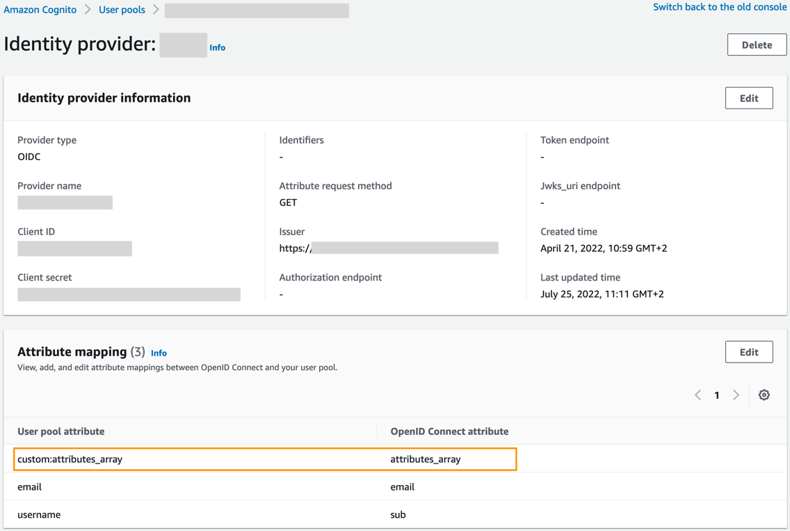
Map IAM roles to OpenSearch Service roles
Upon login, OpenSearch Service maps users to an OpenSearch Service role based on the IAM role ARN set in the cognito:preferred\_role claim by the pre-token generation Lambda trigger. This requires a role mapping in OpenSearch Service. To add such role mappings to IAM backend roles, refer to Mapping roles to users. The following screenshot shows a role mapping on the OpenSearch Dashboards console.

Create the attribute-role mapping table
For this solution, we use DynamoDB to store mappings of users to IAM roles. For instructions, refer to Create a table and define a partition key named Key of type String. You need the table name in the subsequent step to configure the Lambda function.
The next step is writing the mapping information into the table. A mapping entry consists of the following attributes:
- Key – A string that contains attribute values in comma-separated alphabetical order
- RoleArn – A string with the IAM role ARN to which the attribute value combination should be mapped
For details on how to add data to a DynamoDB table, refer to Write data to a table using the console or AWS CLI.
For example, if the previously configured OIDC attribute attributes\_array contains three values, attribute\_a, attribute\_b, and attribute\_c, the entry in the mapping table looks like table line 1 in the following screenshot.

Deploy and configure the pre-token generation Lambda function
A Lambda function implements the custom role mapping logic. The Lambda function receives an Amazon Cognito event as input and extracts attribute information out of it. It uses the attribute information for a lookup in a DynamoDB table and retrieves the value for cognito:preferred\_role. Follow the steps in Getting started with Lambda to create a Node.js Lambda function and insert the following source code:
The Lambda function expects three environment variables. Refer to Using AWS Lambda environment variables for instructions to add the following entries:
- TABLE\_NAME – The name of the previously created DynamoDB table. This table is used for the lookups.
- UNAUTHORIZED\_ROLE – The ARN of the IAM role that is used when no mapping is found in the lookup table.
- USER\_POOL\_ATTRIBUTE – The Amazon Cognito user pool attribute used for the IAM role lookup. In our example, this attribute is named
custom:attributes\_array.
The following screenshot shows the final configuration.

The Lambda function needs permissions to access the DynamoDB lookup table. Set permissions as follows: attach the following policy to the Lambda execution role (for instructions, refer to Lambda execution role) and provide the Region, AWS account number, and DynamoDB table name:
The configuration of the Lambda function is now complete.
Configure the pre-token generation Lambda trigger
As final step, add a pre-token generation trigger to the Amazon Cognito user pool and reference the newly created Lambda function. For details, refer to Customizing user pool workflows with Lambda triggers. The following screenshot shows the configuration.

This step completes the setup; Amazon Cognito now maps users to OpenSearch Service roles based on the values provided in an OIDC attribute.
Test the login to OpenSearch Dashboards
The following diagram shows an exemplary login flow and the corresponding screenshots for an Okta user user1 with a user profile attribute attribute\_array and value: ["attribute\_a", "attribute\_b", "attribute\_c"].

Clean up
To avoid incurring future charges, delete the OpenSearch Service domain, Amazon Cognito user pool and identity pool, Lambda function, and DynamoDB table created as part of this post.
Conclusion
In this post, we demonstrated how to set up a custom mapping to OpenSearch Service roles using values provided via an OIDC attribute. We dynamically set the cognito:preferred\_role claim using an Amazon Cognito pre-token generation Lambda trigger and a DynamoDB table for lookup. The solution is capable of handling dynamic multivalued user attributes, but you can extend it with further application logic that goes beyond a simple lookup. The steps in this post are a proof of concept. If you plan to develop this into a productive solution, we recommend implementing Okta and AWS security best practices.
The post highlights just one use case of how you can use Amazon Cognito support for Lambda triggers to implement custom authentication needs. If you’re interested in further details, refer to How to Use Cognito Pre-Token Generation trigger to Customize Claims In ID Tokens.
About the Authors
 Stefan Appel is a Senior Solutions Architect at AWS. For 10+ years, he supports enterprise customers adopt cloud technologies. Before joining AWS, Stefan held positions in software architecture, product management, and IT operations departments. He began his career in research on event-based systems. In his spare time, he enjoys hiking and has walked the length of New Zealand following Te Araroa.
 Modood Alvi is Senior Solutions Architect at Amazon Web Services (AWS). Modood is passionate about digital transformation and is committed helping large enterprise customers across the globe accelerate their adoption of and migration to the cloud. Modood brings more than a decade of experience in software development, having held various technical roles within companies like SAP and Porsche Digital. Modood earned his Diploma in Computer Science from the University of Stuttgart.
This post is co-written with Olivia Michele and Dariswan Janweri P. at Ruparupa.
Ruparupa was built by PT. Omni Digitama Internusa with the vision to cultivate synergy and create a seamless digital ecosystem within Kawan Lama Group that touches and enhances the lives of many.
Ruparupa is the first digital platform built by Kawan Lama Group to give the best shopping experience for household, furniture, and lifestyle needs. Ruparupa’s goal is to help you live a better life, shown by the meaning of the word ruparupa, which means “everything.” We believe that everyone deserves the best, and home is where everything starts.
In this post, we show how Ruparupa implemented an incrementally updated data lake to get insights into their business using Amazon Simple Storage Service (Amazon S3), AWS Glue, Apache Hudi, and Amazon QuickSight. We also discuss the benefits Ruparupa gained after the implementation.
The data lake implemented by Ruparupa uses Amazon S3 as the storage platform, AWS Database Migration Service (AWS DMS) as the ingestion tool, AWS Glue as the ETL (extract, transform, and load) tool, and QuickSight for analytic dashboards.
Amazon S3 is an object storage service with very high scalability, durability, and security, which makes it an ideal storage layer for a data lake. AWS DMS is a database migration tool that supports many relational database management services, and also supports Amazon S3.
An AWS Glue ETL job, using the Apache Hudi connector, updates the S3 data lake hourly with incremental data. The AWS Glue job can transform the raw data in Amazon S3 to Parquet format, which is optimized for analytic queries. The AWS Glue Data Catalog stores the metadata, and Amazon Athena (a serverless query engine) is used to query data in Amazon S3.
AWS Secrets Manager is an AWS service that can be used to store sensitive data, enabling users to keep data such as database credentials out of source code. In this implementation, Secrets Manager is used to store the configuration of the Apache Hudi job for various tables.
Data analytic challenges
As an ecommerce company, Ruparupa produces a lot of data from their ecommerce website, their inventory systems, and distribution and finance applications. The data can be structured data from existing systems, and can also be unstructured or semi-structured data from their customer interactions. This data contains insights that, if unlocked, can help management make decisions to help increase sales and optimize cost.
Before implementing a data lake on AWS, Ruparupa had no infrastructure capable of processing the volume and variety of data formats in a short time. Data had to be manually processed by data analysts, and data mining took a long time. Because of the fast growth of data, it took 1–1.5 hours just to ingest data, which was hundreds of thousands of rows.
The manual process caused inconsistent data cleansing. After the data had been cleansed, some processes were often missing, and all the data had to go through another process of data cleansing.
This long processing time reduced the analytic team’s productivity. The analytic team could only produce weekly and monthly reports. This delay in report frequency impacted delivering important insights to management, and they couldn’t move fast enough to anticipate changes in their business.
The method used to create analytic dashboards was manual and could only produce a few routine reports. The audience of these few reports was limited—a maximum of 20 people from management. Other business units in Kawan Lama Group only consumed weekly reports that were prepared manually. Even the weekly reports couldn’t cover all important metrics, because some metrics were only available in monthly reports.
Initial solution for a real-time dashboard
The following diagram illustrates the initial solution Ruparupa implemented.

Ruparupa started a data initiative within the organization to create a single source of truth within the company. Previously, business users could only get the sales data from the day before, and they didn’t have any visibility to current sales activities in their stores and websites.
To gain trust from business users, we wanted to provide the most updated data in an interactive QuickSight dashboard. We used an AWS DMS replication task to stream real-time change data capture (CDC) updates to an Amazon Aurora MySQL-Compatible Edition database, and built a QuickSight dashboard to replace the static presentation deck.
This pilot dashboard was accepted extremely well by the users, who now had visibility to their current data. However, the data source for the dashboard still resided in an Aurora MySQL database and only covered a single data domain.
The initial design had some additional challenges:
- Diverse data source – The data source in an ecommerce platform consists of structured, semi-structured, and unstructured data, which requires flexible data storage. The initial data warehouse design in Ruparupa only stored transactional data, and data from other systems including user interaction data wasn’t consolidated yet.
- Cost and scalability – Ruparupa wanted to build a future-proof data platform solution that could scale up to terabytes of data in the most cost-effective way.
The initial design also had some benefits:
- Data updates – Data inside the initial data warehouse was delayed by 1 day. This was an improvement over the weekly report, but still not fast enough to make quicker decisions.
This solution only served as a temporary solution; we needed a more complete analytics solution that could serve more complex and larger data sources, faster, and cost-effectively.
Real-time data lake solution
To fulfill their requirements, Ruparupa introduced a mutable data lake, as shown in the following diagram.

Let’s look at each main component in more detail.
AWS DMS CDC process
To get the real-time data from the source, we streamed the database CDC log using AWS DMS (component 1 in the architecture diagram). The CDC records consist of all inserts, updates, and deletes from the source database. This raw data is stored in the raw layer of the S3 data lake.
An S3 lifecycle policy is used to manage data retention, where the older data is moved to Amazon S3 Glacier.
AWS Glue ETL job
The second S3 data lake layer is the transformed layer, where the data is transformed to an optimized format that is ready for user query. The files are transformed to Parquet columnar format with snappy compression and table partitioning to optimize SQL queries from Athena.
In order to create a mutable data lake that can merge changes from the data source, we introduced an Apache Hudi data lake framework. With Apache Hudi, we can perform upserts and deletes on the transformed layer to keep the data consistent in a reliable manner. With a Hudi data lake, Ruparupa can create a single source of truth for all our data sources quickly and easily. The Hudi framework takes care of the underlying metadata of the updates, making it simple to implement across hundreds of tables in the data lake. We only need to configure the writer output to create a copy-on-write table depending on the access requirements. For the writer, we use an AWS Glue job writer combined with an AWS Glue Hudi connector frrom AWS Marketplace. The additional library from the connector helps AWS Glue understand how to write to Hudi.
An AWS Glue ETL job is used to get the changes from the raw layer and merge the changes in the transformed layer (component 2 in the architecture diagram). With AWS Glue, we are able to create a PySpark job to get the data, and we use the AWS Glue Connector for Apache Hudi to simplify the Hudi library import to the AWS Glue job. With AWS Glue, all the changes from AWS DMS can be merged easily to the Hudi data lake. The jobs are scheduled every hour using a built-in scheduler in AWS Glue.
Secrets Manager is used to store all the related parameters that are required to run the job. Instead of making one transformation job for each table, Ruparupa creates a single generic job that can transform multiple tables by using several parameters. The parameters that give details about the table structure are stored in Secrets Manager and can be retrieved using the name of the table as key. With these custom parameters, Ruparupa doesn’t need to create a job for every table—we can utilize a single job that can ingest the data for all different tables by passing the name of the table to the job.
All the metadata of the tables is stored in the AWS Glue Data Catalog, including the Hudi tables. This catalog is used by the AWS Glue ETL job, Athena query engine, and QuickSight dashboard.
Athena queries
Users can then query the latest data for their report using Athena (component 3 in the architecture diagram). Athena is serverless, so there is no infrastructure to provision or maintain. We can immediately use SQL to query the data lake to create a report or ingest the data to the dashboard.
QuickSight dashboard
Business users can use a QuickSight dashboard to query the data lake (component 4 in the architecture diagram). The existing dashboard is modified to get data from Athena, replacing the previous database. New dashboards were also created to fulfill continuously evolving needs for insights from multiple business units.
QuickSight is also used to notify certain parties when a value is reaching a certain threshold. An email alert is sent to an external notification and messaging platform so it can reach the end-user.
Business results
The data lake implementation in Ruparupa took around 3 months, with an additional month for data validation, before it was considered ready for production. With this solution, management can get the latest information view of their current state up to the last 1 hour. Previously, they could only generate weekly reports—now insights are available 168 times faster.
The QuickSight dashboard, which can be updated automatically, shortens the time required by the analytic team. The QuickSight dashboard now has more content—not only is transactional data reported, but also other metrics like new SKU, operation escalation for free services to customers, and monitoring SLA. Since April 2021 when Ruparupa started their QuickSight pilot, the number of dashboards has increased to around 70 based on requests from business users.
Ruparupa has hired new personnel to join the data analytic team to explore new possibilities and new use cases. The analytic team has grown from just one person to seven to handle new analytic use cases:
- Merchandising
- Operations
- Store manager performance measurement
- Insights of trending SKUs
Kawan Lama Group also has offline stores besides the ecommerce platform managed by Ruparupa. With the new dashboard, it’s easier to compare transaction data from online and offline stores because they now use the same platform.
The new dashboards also can be consumed by a broader audience, including other business units in Kawan Lama Group. The total users consuming the dashboard increased from just 20 users from management to around 180 users (9 times increase).
Since the implementation, other business units in Kawan Lama Group have increased their trust in the S3 data lake platform implemented by Ruparupa, because the data is more up to date and they can drill down to the SKU level to validate that the data is correct. Other business units can now act faster after an event like a marketing campaign. This data lake implementation has helped increase sales revenue in various business units in Kawan Lama Group.
Conclusion
Implementing a real-time data lake using Amazon S3, Apache Hudi, AWS Glue, Athena, and QuickSight gave Ruparupa the following benefits:
- Yielded faster insights (hourly compared to weekly)
- Unlocked new insights
- Enabled more people in more business units to consume the dashboard
- Helped business units in Kawan Lama Group act faster and increase sales revenue
If you’re interested in gaining similar benefits, check out Build a Data Lake Foundation with AWS Glue and Amazon S3.
You can also learn how to get started with QuickSight in the Getting Started guide.
Last but not least, you can learn about running Apache Hudi on AWS Glue in Writing to Apache Hudi tables using AWS Glue Custom Connector.
About the Authors
 Olivia Michele is a Data Scientist Lead at Ruparupa, where she has worked in a variety of data roles over the past 5 years, including building and integrating Ruparupa data systems with AWS to improve user experience with data and reporting tools. She is passionate about turning raw information into valuable actionable insights and delivering value to the company.
 Dariswan Janweri P. is a Data Engineer at Ruparupa. He considers challenges or problems as interesting riddles and finds satisfaction in solving them, and even more satisfaction by being able to help his colleagues and friends, “two birds one stone.” He is excited to be a major player in Indonesia’s technology transformation.
 Adrianus Budiardjo Kurnadi is a Senior Solutions Architect at Amazon Web Services Indonesia. He has a strong passion for databases and machine learning, and works closely with the Indonesian machine learning community to introduce them to various AWS Machine Learning services. In his spare time, he enjoys singing in a choir, reading, and playing with his two children.
 Nico Anandito is an Analytics Specialist Solutions Architect at Amazon Web Services Indonesia. He has years of experience working in data integration, data warehouses, and big data implementation in multiple industries. He is certified in AWS data analytics and holds a master’s degree in the data management field of computer science.
Data warehouses play a vital role in healthcare decision-making and serve as a repository of historical data. A healthcare data warehouse can be a single source of truth for clinical quality control systems. Data warehouses are mostly built using the dimensional model approach, which has consistently met business needs.
Loading complex multi-point datasets into a dimensional model, identifying issues, and validating data integrity of the aggregated and merged data points are the biggest challenges that clinical quality management systems face. Additionally, scalability of the dimensional model is complex and poses a high risk of data integrity issues.
The data vault approach solves most of the problems associated with dimensional models, but it brings other challenges in clinical quality control applications and regulatory reports. Because data is closer to the source and stored in raw format, it has to be transformed before it can be used for reporting and other application purposes. This is one of the biggest hurdles with the data vault approach.
In this post, we discuss some of the main challenges enterprise data warehouses face when working with dimensional models and data vaults. We dive deep into a hybrid approach that aims to circumvent the issues posed by these two and also provide recommendations to take advantage of this approach for healthcare data warehouses using Amazon Redshift.
What is a dimensional data model?
Dimensional modeling is a strategy for storing data in a data warehouse using dimensions and facts. It optimizes the database for faster data retrieval. Dimensional models have a distinct structure and organize data to provide reports that increase performance.
In a dimensional model, a transaction record is divided either into facts (often numerical), additive transactional data, or dimensions (referential information that gives context to the facts). This categorization of data into facts and dimensions, as well as the entity-relationship framework of the dimensional model, presents complex business processes in a way that is easy for analysts to understand.
A dimensional model in data warehousing is designed for reading, summarizing, and analyzing numerical information such as patient vital stats, lab reading values, counts, and so on. Regardless of the division or use case it is related to, dimensional data models can be used to store data obtained from tracking various processes like patient encounters, provider practice metrics, aftercare surveys, and more.
The majority of healthcare clinical quality data warehouses are built on top of dimensional modeling techniques. The benefit of using dimensional data modeling is that, when data is stored in a data warehouse, it’s easier to persist and extract it.
Although it’s a competent data structure technique, there are challenges in scalability, source tracking, and troubleshooting with the dimensional modeling approach. Tracking and validating the source of aggregated and compute data points is important in clinical quality regulatory reporting systems. Any mistake in regulatory reports may result in a large penalty from regulatory and compliance agencies. These challenges exist because the data points are labeled using meaningless numeric surrogate keys, and any minor error can impair prediction accuracy, and consequently affect the quality of judgments. The ways to countervail these challenges are by refactoring and bridging the dimensions. But that adds data noise over time and reduces accuracy.
Let’s look at an example of a typical dimensional data warehouse architecture in healthcare, as shown in the following logical model.

The following diagram illustrates a sample dimensional model entity-relationship diagram.

This data model contains dimensions and fact tables. You can use the following query to retrieve basic provider and patient relationship data from the dimensional model:
Challenges of dimensional modeling
Dimensional modeling requires data preprocessing before generating a star schema, which involves a large amount of data processing. Any change to the dimension definition results in a lengthy and time-consuming reprocessing of the dimension data, which often results in data redundancy.
Another issue is that, when relying merely on dimensional modeling, analysts can’t assure the consistency and accuracy of data sources. Especially in healthcare, where lineage, compliance, history, and traceability are of prime importance because of the regulations in place.
A data vault seeks to provide an enterprise data warehouse while solving the shortcomings of dimensional modeling approaches. It is a data modeling methodology designed for large-scale data warehouse platforms.
What is a data vault?
The data vault approach is a method and architectural framework for providing a business with data analytics services to support business intelligence, data warehousing, analytics, and data science needs. The data vault is built around business keys (hubs) defined by the company; the keys obtained from the sources are not the same.
Amazon Redshift RA3 instances and Amazon Redshift Serverless are perfect choices for a data vault. And when combined with Amazon Redshift Spectrum, a data vault can deliver more value.
There are three layers to the data vault:
- Staging
- Data vault
- Business vault
Staging involves the creation of a replica of the original data, which is primarily used to aid the process of transporting data from various sources to the data warehouse. There are no restrictions on this layer, and it is typically not persistent. It is 1:1 with the source systems, generally in the same format as that of the sources.
The data vault is based on business keys (hubs), which are defined by the business. All in-scope data is loaded, and auditability is maintained. At the heart of all data warehousing is integration, and this layer contains integrated data from multiple sources built around the enterprise-wide business keys. Although data lakes resemble data vaults, a data vault provides more features of a data warehouse. However, it combines the functionalities of both.
The business vault stores the outcome of business rules, including deduplication, conforming results, and even computations. When results are calculated for two or more data marts, this helps eliminate redundant computation and associated inconsistencies.
Because business vaults still don’t satisfy reporting needs, enterprises create a data mart after the business vault to satisfy dashboarding needs.
Data marts are ephemeral views that can be implemented directly on top of the business and raw vaults. This makes it easy to adapt over time and eliminates the danger of inconsistent results. If views don’t give the required level of performance, the results can be stored in a table. This is the presentation layer and is designed to be requirements-driven and scope-specific subsets of the warehouse data. Although dimensional modeling is commonly used to deliver this layer, marts can also be flat files, .xml files, or in other forms.
The following diagram shows the typical data vault model used in clinical quality repositories.

When the dimensional model as shown earlier is converted into a data vault using the same structure, it can be represented as follows.
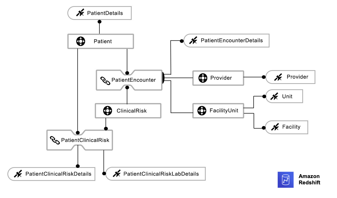
Advantages of a data vault
Although any data warehouse should be built within the context of an overarching company strategy, data vaults permit incremental delivery. You can start small and gradually add more sources over time, just like Kimball’s dimensional design technique.
With a data vault, you don’t have to redesign the structure when adding new sources, unlike dimensional modeling. Business rules can be easily changed because raw and business-generated data is kept independent of each other in a data vault.
A data vault isolates technical data reorganization from business rules, thereby facilitating the separation of these potentially tricky processes. Similarly, data cleaning can be maintained separately from data import.
A data vault accommodates changes over time. Unlike a pure dimensional design, a data vault separates raw and business-generated data and accepts changes from both sources.
Data vaults make it easy to maintain data lineage because it includes metadata identifying the source systems. In contrast to dimensional design, where data is cleansed before loading, data vault updates are always gradual, and results are never lost, providing an automatic audit trail.
When raw data is stored in a data vault, historical attributes that weren’t initially available can be added to the presentation area. Data marts can be implemented as views by adding a new column to an existing view.
In data vault 2.0, hash keys eliminate data load dependencies, which allows near-real-time data loading, as well as concurrent data loads of terabytes to petabytes. The process of mastering both entity-relationship modeling and dimensional design takes time and practice, but the process of automating a data vault is easier.
Challenges of a data vault
A data vault is not a one-size-fits-all solution for data warehouses, and it does have a few limitations.
To begin with, when directly feeding the data vault model into a report on one subject area, you need to combine multiple types of data. Due to the incapability of reporting technologies to perform such data processing, this integration can reduce report performance and increase the risk of errors. However, data vault models could improve report performance by incorporating dimensional models or adding additional reporting layers. And for data models that can be directly reported, a dimensional model can be developed.
Additionally, if the data is static or if it comes from a single source, it reduces the efficacy of data vaults. They often negate many benefits of data vaults, and require more business logic, which can be avoided.
The storage requirement for a data vault is also significantly higher. Three separate tables for the same subject area can effectively increase the number of tables by three, and when they are inserts only. If the data is basic, you can achieve the benefits listed here with a simpler dimensional model rather than deploying a data vault.
The following sample query retrieves provider and patient data from a data vault using the sample model we discussed in this section:
The query involves many joins, which increases the depth and time for the query run, as illustrated in the following chart.

This following table shows that the SQL depth and runtime is proportional, where depth is the number of joins. If the number of joins increase, then the runtime also increases and therefore the cost.
| SQL Depth | Runtime in Seconds | Cost per Query in Seconds |
| 14 | 80 | 40,000 |
| 12 | 60 | 30,000 |
| 5 | 30 | 15,000 |
| 3 | 25 | 12,500 |
The hybrid model addresses major issues raised by the data vault and dimensional model approaches that we’ve discussed in this post, while also allowing improvements in data collection, including IoT data streaming.
What is a hybrid model?
The hybrid model combines the data vault and a portion of the star schema to provide the advantages of both the data vault and dimensional model, and is mainly intended for logical enterprise data warehouses.
The hybrid approach is designed from the bottom up to be gradual and modular, and it can be used for big data, structured, and unstructured datasets. The primary data contains the business rules and enterprise-level data standards norms, as well as additional metadata needed to transform, validate, and enrich data for dimensional approaches. In this model, data processes from left to right provide data vault advantages, and data processes from right to left provide dimensional model advantages. Here, the data vault satellite tables serve as both satellite tables and dimensional tables.
After combining the dimensional and the data vault models, the hybrid model can be viewed as follows.

The following is an example entity-relation diagram of the hybrid model, which consists of a fact table from the dimensional model and all other entities from the data vault. The satellite entity from the data vault plays the dual role. When it’s connected to a data vault, it acts as a sat table, and when connected to a fact table, it acts as a dimension table. To serve this dual purpose, sat tables have two keys: a foreign key to connect with the data vault, and a primary key to connect with the fact table.
The following diagram illustrates the physical hybrid data model.

The following diagram illustrates a typical hybrid data warehouse architecture.

The following query retrieves provider and patient data from the hybrid model:
The number of joins is reduced from five to three by using the hybrid model.
Advantages of using the hybrid model
With this model, structural information is segregated from descriptive information to promote flexibility and avoid re-engineering in the event of a change. It maintains data integrity, allowing organizations to avoid hefty fines when data integrity is compromised.
The hybrid paradigm enables non-data professionals to interact with raw data by allowing users to update or create metadata and data enrichment rules. The hybrid approach simplifies the process of gathering and evaluating datasets for business applications. It enables concurrent data loading and eliminates the need for a corporate vault.
The hybrid model also benefits from the fact that there is no dependency between objects in the data storage. With hybrid data warehousing, scalability is multiplied.
You can build the hybrid model on AWS and take advantage of the benefits of Amazon Redshift, which is a fully managed, scalable cloud data warehouse that accelerates your time to insights with fast, simple, and secure analytics at scale. Amazon Redshift continuously adds features that make it faster, more elastic, and easier to use:
- Amazon Redshift data sharing enhances the hybrid model by eliminating the need for copying data across departments. It also simplifies the work of keeping the single source of truth, saving memory and limiting redundancy. It enables instant, granular, and fast data access across Amazon Redshift clusters without the need to copy or move it. Data sharing provides live access to data so that users always see the most up-to-date and consistent information as it’s updated in the data warehouse.
- Redshift Spectrum enables you to query open format data directly in the Amazon Simple Storage Service (Amazon S3) data lake without having to load the data or duplicate your infrastructure, and it integrates well with the data lake.
- With Amazon Redshift concurrency scaling, you can get consistently fast performance for thousands of concurrent queries and users. It instantly adds capacity to support additional users and removes it when the load subsides, with nothing to manage at your end.
- To realize the benefits of using a hybrid model on AWS, you can get started today without needing to provision and manage data warehouse clusters using Redshift Serverless. All the related services that Amazon Redshift integrates with (such as Amazon Kinesis, AWS Lambda, Amazon QuickSight, Amazon SageMaker, Amazon EMR, AWS Lake Formation, and AWS Glue) are available to work with Redshift Serverless.
Conclusion
With the hybrid model, data can be transformed and loaded into a target data model efficiently and transparently. With this approach, data partners can research data networks more efficiently and promote comparative effectiveness. And with the several newly introduced features of Amazon Redshift, a lot of heavy lifting is done by AWS to handle your workload demands, and you only pay for what you use.
You can get started with the following steps:
- Create an Amazon Redshift RA3 instance for your primary clinical data repository and data marts.
- Build a data vault schema for the raw vault and create materialized views for the business vault.
- Enable Amazon Redshift data shares to share data between the producer cluster and consumer cluster.
- Load the structed and unstructured data into the producer cluster data vault for business use.
About the Authors
 Bindhu Chinnadurai is a Senior Partner Solutions Architect in AWS based out of London, United Kingdom. She has spent 18+ years working in everything for large scale enterprise environments. Currently she engages with AWS partner to help customers migrate their workloads to AWS with focus on scalability, resiliency, performance and sustainability. Her expertise is DevSecOps.
 Sarathi Balakrishnan was the Global Partner Solutions Architect, specializing in Data, Analytics and AI/ML at AWS. He worked closely with AWS partner globally to build solutions and platforms on AWS to accelerate customers’ business outcomes with state-of-the-art cloud technologies and achieve more in their cloud explorations. He helped with solution architecture, technical guidance, and best practices to build cloud-native solutions. He joined AWS with over 20 years of large enterprise experience in agriculture, insurance, health care and life science, marketing and advertisement industries to develop and implement data and AI strategies.
This post was co-written with Django Bouchez, Solution Engineer at Toucan.
Business intelligence (BI) with dashboards, reports, and analytics remains one of the most popular use cases for data and analytics. It provides business analysts and managers with a visualization of the business’s past and current state, helping leaders make strategic decisions that dictate the future. However, customers continue to ask for better ways to tell stories with their data, and therefore increase the adoption rate of their BI tools.
Most BI tools on the market provide an exhaustive set of customization options to build data visualizations. It might appear as a good idea, but ultimately burdens business analysts that need to navigate through endless possibilities before building a report. Analysts are not graphic designers, and a poorly designed data visualization can hide the insight it’s intended to convey, or even mislead the viewer. To realize more value from your data, you should focus on building data visualizations that tell stories, and are easily understandable by your audience. This is where guided analytics helps. Instead of presenting unlimited options for customization, it intentionally limits choice by enforcing design best practices. The simplicity of a guided experience enables business analysts to spend more time generating actual insight rather than worrying about how to present them.
This post illustrates the concept of guided analytics and shows you how you can build a data storytelling application with Amazon Redshift Serverless and Toucan, an AWS Partner. Toucan natively integrates with Redshift Serverless, which enables you to deploy a scalable data stack in minutes without the need to manage any infrastructure component.
Amazon Redshift is a fully managed cloud data warehouse service that enables you to analyze large amounts of structured and semi-structured data. Amazon Redshift can scale from a few gigabytes to a petabyte-scale data warehouse, and AWS recently announced the global availability of Redshift Serverless, making it one of the best options for storing data and running ad hoc analytics in a scalable and cost-efficient way.
With Redshift Serverless, you can get insights on your data by running standalone SQL queries or by using data visualizations tools such as Amazon QuickSight, Toucan, or other third-party options without having to manage your data warehouse infrastructure.
Toucan is a cloud-based guided analytics platform built with one goal in mind: reduce the complexity of bringing data insights to business users. For this purpose, Toucan provides a no-code and comprehensive user experience at every stage of the data storytelling application, which includes data connection, building the visualization, and distribution on any device.
If you’re in a hurry and want to see what you can do with this integration, check out Shark attacks visualization with AWS & Toucan, where Redshift Serverless and Toucan help in understanding the evolution of shark attacks in the world.
Overview of solution
There are many BI tools in the market, each providing an ever-increasing set of capabilities and customization options to differentiate from the competition. Paradoxically, this doesn’t seem to increase the adoption rate of BI tools in enterprises. With more complex tools, data owners spend time building fancy visuals, and tend to add as much information as possible in their dashboards instead of providing a clear and simple message to business users.
In this post, we illustrate the concept of guided analytics by putting ourselves in the shoes of a data engineer that needs to communicate stories to business users with data visualizations. This fictional data engineer has to create dashboards to understand how shark attacks evolved in the last 120 years. After loading the shark attacks dataset in Redshift Serverless, we guide you in using Toucan to build stories that provide a better understanding of shark attacks through time. With Toucan, you can natively connect to datasets in Redshift Serverless, transform the data with a no-code interface, build storytelling visuals, and publish them for business users. The shark attacks visualization example illustrates what you can achieve by following instructions in this post.
Additionally, we have recorded a video tutorial that explains how to connect Toucan with Redshift Serverless and start building charts.
Solution architecture
The following diagram depicts the architecture of our solution.
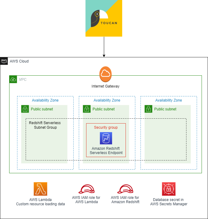
We use an AWS CloudFormation stack to deploy all the resources you need in your AWS account:
- Networking components – This includes a VPC, three public subnets, an internet gateway, and a security group to host the Redshift Serverless endpoint. In this post, we use public subnets to facilitate data access from external sources such as Toucan instances. In this case, the data in Redshift Serverless is still protected by the security group that restricts incoming traffic, and by the database credentials. For a production workload, it is recommended to keep traffic in the Amazon network. For that, you can set the Redshift Serverless endpoints in private subnets, and deploy Toucan in your AWS account through the AWS Marketplace.
- Redshift Serverless components – This includes a Redshift Serverless namespace and workgroup. The Redshift Serverless workspace is publicly accessible to facilitate the connection from Toucan instances. The database name and the administrator user name are defined as parameters when deploying the CloudFormation stack, and the administrator password is created in AWS Secrets Manager. In this post, we use database credentials to connect to Redshift Serverless, but Toucan also supports connection with AWS credentials and AWS Identity and Access Management (IAM) profiles.
- Custom resources – The CloudFormation stack includes a custom resource, which is an AWS Lambda function that loads shark attacks data automatically in your Redshift Serverless database when the CloudFormation stack is created.
- IAM roles and permissions – Finally, the CloudFormation stack includes all IAM roles associated with services previously mentioned to interact with other AWS resources in your account.
In the following sections, we provide all the instructions to connect Toucan with your data in Redshift Serverless, and guide you to build your data storytelling application.
Sample dataset
In this post, we use a custom dataset that lists all known shark attacks in the world, starting from 1900. You don’t have to import the data yourself; we use the Amazon Redshift COPY command to load the data when deploying the CloudFormation stack. The COPY command is one the fastest and most scalable methods to load data into Amazon Redshift. For more information, refer to Using a COPY command to load data.
The dataset contains 4,900 records with the following columns:
- Date
- Year
- Decade
- Century
- Type
- Zone\_Type
- Zone
- Country
- Activity
- Sex
- Age
- Fatal
- Time
- Species
- href (a PDF link with the description of the context)
- Case\_Number
Prerequisites
For this solution, you should have the following prerequisites:
- An AWS account. If you don’t have one already, see the instructions in Sign Up for AWS.
- An IAM user or role with permissions on AWS resources used in this solution.
- A Toucan free trial to build the data storytelling application.
Set up the AWS resources
You can launch the CloudFormation stack in any Region where Redshift Serverless is available.
- Choose Launch Stack to start creating the required AWS resources for this post:
- Specify the database name in Redshift Serverless (default is
dev). - Specify the administrator user name (default is
admin).
You don’t have to specify the database administrator password because it’s created in Secrets Manager by the CloudFormation stack. The secret’s name is AWS-Toucan-Redshift-Password. We use the secret value in subsequent steps.
Test the deployment
The CloudFormation stack takes a few minutes to deploy. When it’s complete, you can confirm the resources were created. To access your data, you need to get the Redshift Serverless database credentials.
- On the Outputs tab for the CloudFormation stack, note the name of the Secrets Manager secret.

- On the Secrets Manager console, navigate to the Amazon Redshift database secret and choose Retrieve secret value to get the database administrator user name and password.
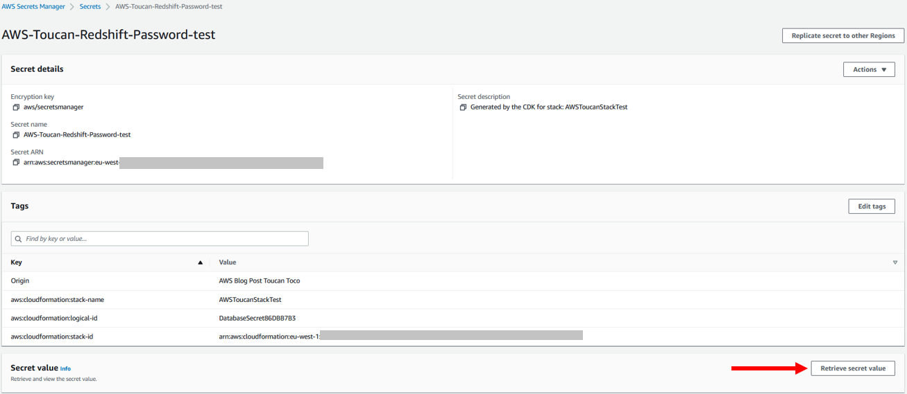
- To make sure your Redshift Serverless database is available and contains the shark attacks dataset, open the Redshift Serverless workgroup on the Amazon Redshift console and choose Query data to access the query editor.
- Also note the Redshift Serverless endpoint, which you need to connect with Toucan.

- In the Amazon Redshift query editor, run the following SQL query to view the shark attacks data:
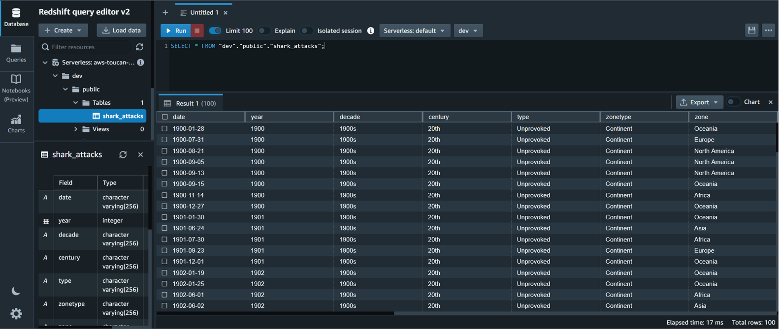
Note that you need to change the name of the database in the SQL query if you change the default value when launching the CloudFormation stack.
You have configured Redshift Serverless in your AWS account and uploaded the shark attacks dataset. Now it’s time to use this data by building a storytelling application.
Launch your Toucan free trial
The first step is to access Toucan platform through the Toucan free trial.
Fill the form and complete the signup steps. You then arrive in the Storytelling Studio, in Staging mode. Feel free to explore what has been already created.
Connect Redshift Serverless with Toucan
To connect Redshift Serverless and Toucan, complete the following steps:
- Choose Datastore at the bottom of the Toucan Storytelling Studio.
- Choose Connectors.
Toucan is natively integrated with Redshift Serverless with AnyConnect.
- Search for the Amazon Redshift connector, and complete the form with the following information:
- Name – The name of the connector in Toucan.
- Host – Your Redshift Serverless endpoint.
- Port – The listening port of your Amazon Redshift database (5439).
- Default Database – The name of the database to connect to (dev by default, unless edited in the CloudFormation stack parameters).
- Authentication Method – The authentication mechanism to connect to Redshift Serverless. In this case, we use database credentials.
- User – The user name to use for authentication with Redshift Serverless (admin by default, unless edited in the CloudFormation stack parameters).
- Password – The password to use for authentication with Redshift Serverless (you should retrieve it from Secrets Manager; the secret’s name is
AWS-Toucan-Redshift-Password).
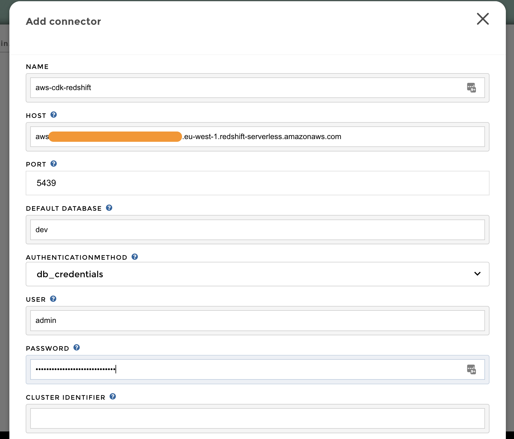
Create a live query
You are now connected to Redshift Serverless. Complete the following steps to create a query:
- On the home page, choose Add tile to create a new visualization.

- Choose the Live Connections tab, then choose the Amazon Redshift connector you created in the previous step.
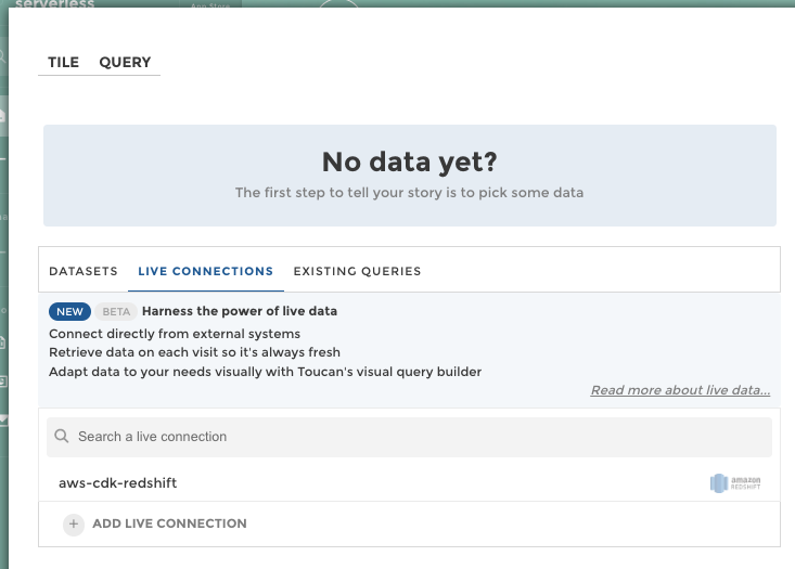
The Toucan trial guides you in building your first live query, in which you can transform your data without writing code using the Toucan YouPrep module.
For instance, as shown in the following screenshot, you can use this no-code interface to compute the sum of fatal shark attacks by activities, get the top five, and calculate the percentage of the total.
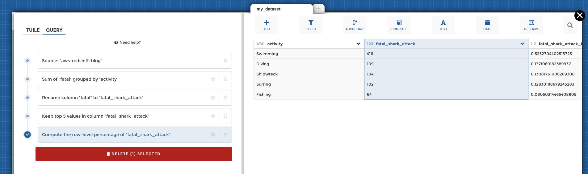
Build your first chart
When your data is ready, choose the Tile tab and complete the form that helps you build charts.
For example, you can configure a leaderboard of the five most dangerous activities, and add a highlight for activities with more than 100 attacks.
Choose Save Changes to save your work and go back to the home page.

Publish and share your work
Until this stage, you have been working in working in Staging mode. To make your work available to everyone, you need to publish it into Production.
On the bottom right of the home page, choose the eye icon to preview your work by putting yourself in the shoes of your future end-users. You can then choose Publish to make your work available to all.
Toucan also offers multiple embedding options to make your charts easier for end-users to access, such as mobile and tablet.
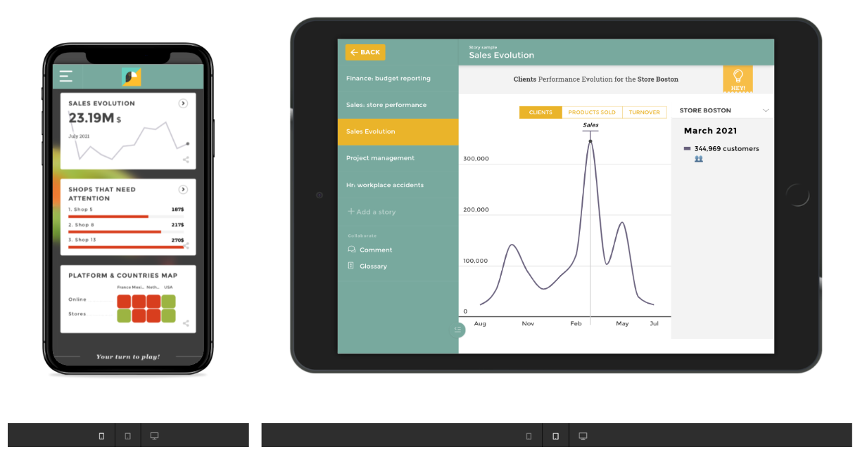
Following these steps, you connected to Redshift Serverless, transformed the data with the Toucan no-code interface, and built data visualizations for business end-users. The Toucan trial guides you in every stage of this process to help you get started.
Redshift Serverless and Toucan guided analytics provide an efficient approach to increase the adoption rate of BI tools by decreasing infrastructure work for data engineers, and by simplifying dashboard understanding for business end-users. This post only covered a small part of what Redshift Serverless and Toucan offer, so feel free to explore other functionalities in the Amazon Redshift Serverless documentation and Toucan documentation.
Clean up
Some of the resources deployed in this post through the CloudFormation template incur costs as long as they’re in use. Be sure to remove the resources and clean up your work when you’re finished in order to avoid unnecessary cost.
On the CloudFormation console, choose Delete stack to remove all resources.
Conclusion
This post showed you how to set up an end-to-end architecture for guided analytics with Redshift Serverless and Toucan.
This solution benefits from the scalability of Redshift Serverless, which enables you to store, transform, and expose data in a cost-efficient way, and without any infrastructure to manage. Redshift Serverless natively integrates with Toucan, a guided analytics tool designed to be used by everyone, on any device.
Guided analytics focuses on communicating stories through data reports. By setting intentional constraints on customization options, Toucan makes it easy for data owners to build meaningful dashboards with a clear and concise message for end-users. It works for both your internal and external customers, on an unlimited number of use cases.
Try it now with our CloudFormation template and a free Toucan trial!
About the Authors
 Louis Hourcade is a Data Scientist in the AWS Professional Services team. He works with AWS customer across various industries to accelerate their business outcomes with innovative technologies. In his spare time he enjoys running, climbing big rocks, and surfing (not so big) waves.
 Benjamin Menuet is a Data Architect with AWS Professional Services. He helps customers develop big data and analytics solutions to accelerate their business outcomes. Outside of work, Benjamin is a trail runner and has finished some mythic races like the UTMB.
 Xavier Naunay is a Data Architect with AWS Professional Services. He is part of the AWS ProServe team, helping enterprise customers solve complex problems using AWS services. In his free time, he is either traveling or learning about technology and other cultures.
 Django Bouchez is a Solution Engineer at Toucan. He works alongside the Sales team to provide support on technical and functional validation and proof, and is also helping R&D demo new features with Cloud Partners like AWS. Outside of work, Django is a homebrewer and practices scuba diving and sport climbing.
This is a guest post by Nan Zhu, Tech Lead Manager, SafeGraph, and Dave Thibault, Sr. Solutions Architect – AWS
SafeGraph is a geospatial data company that curates over 41 million global points of interest (POIs) with detailed attributes, such as brand affiliation, advanced category tagging, and open hours, as well as how people interact with those places. We use Apache Spark as our main data processing engine and have over 1,000 Spark applications running over massive amounts of data every day. These Spark applications implement our business logic ranging from data transformation, machine learning (ML) model inference, to operational tasks.
SafeGraph found itself with a less-than-optimal Spark environment with their incumbent Spark vendor. Their costs were climbing. Their jobs would suffer frequent retries from Spot Instance termination. Developers spent too much time troubleshooting and changing job configurations and not enough time shipping business value code. SafeGraph needed to control costs, improve developer iteration speed, and improve job reliability. Ultimately, SafeGraph chose Amazon EMR on Amazon EKS to meet their needs and realized 50% savings relative to their previous Spark managed service vendor.
If building Spark applications for our product is like cutting a tree, having a sharp saw becomes crucial. The Spark platform is the saw. The following figure highlights the engineering workflow when working with Spark, and the Spark platform should support and optimize each action in the workflow. The engineers usually start with writing and building the Spark application code, then submit the application to the computing infrastructure, and finally close the loop by debugging the Spark applications. Additionally, platform and infrastructure teams need to continually operate and optimize the three steps in the engineering workflow.
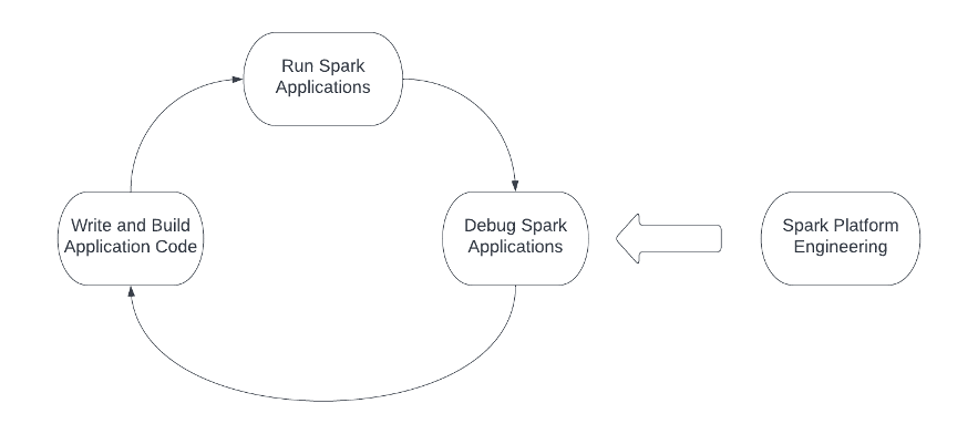
There are various challenges involved in each action when building a Spark platform:
- Reliable dependency management – A complicated Spark application usually brings many dependencies. To run a Spark application, we need to identify all dependencies, resolve any conflicts, pack dependent libraries reliably, and ship them to the Spark cluster. Dependency management is one of the biggest challenges for engineers, especially when they work with PySpark applications.
- Reliable computing infrastructure – The reliability of the computing infrastructure hosting Spark applications is the foundation of the whole Spark platform. Unstable resource provisioning will not only cause negative impact over engineering efficiency, but it will also increase infrastructure costs due to reruns of the Spark applications.
- Convenient debugging tools for Spark applications – The debugging tooling plays a key role for engineers to iterate fast on Spark applications. Performant access to the Spark History Server (SHS) is a must for developer iteration speed. Conversely, poor SHS performance slows developers and increases the cost of goods sold for software companies.
- Manageable Spark infrastructure – A successful Spark platform engineering involves multiple aspects, such as Spark distribution version management, computing resource SKU management and optimization, and more. It largely depends on whether the Spark service vendors provide the right foundation for platform teams to use. The wrong abstraction over distribution version and computing resources, for example, could significantly reduce the ROI of platform engineering.
At SafeGraph, we experienced all of the aforementioned challenges. To resolve them, we explored the marketplace and found that building a new Spark platform on top of EMR on EKS was the solution to our roadblocks. In this post, we share our journey of building our latest Spark platform and how EMR on EKS serves as a robust and efficient foundation for it.
Reliable Python dependency management
One of the biggest challenges for our users to write and build Spark application code is the struggle of managing dependencies reliably, especially for PySpark applications. Most of our ML-related Spark applications are built with PySpark. With our previous Spark service vendor, the only supported way to manage Python dependencies was via a wheel file. Despite its popularity, wheel-based dependency management is fragile. The following figure shows two types of reliability issues faced with wheel-based dependency management:
- Unpinned direct dependency – If the .whl file doesn’t pinpoint the version of a certain direct dependency, Pandas in this example, it will always pull the latest version from upstream, which may potentially contain a breaking change and take down our Spark applications.
- Unpinned transitive dependency – The second type of reliability issue is more out of our control. Even though we pinned the direct dependency version when building the .whl file, the direct dependency itself could miss pinpointing the transitive dependencies’ versions (MLFlow in this example). The direct dependency in this case always pulls the latest versions of these transitive dependencies that potentially contain breaking changes and may take down our pipelines.

The other issue we encountered was the unnecessary installation of all Python packages referred by the wheel files for every Spark application initialization. With our previous setup, we needed to run the installation script to install wheel files for every Spark application upon starting even if there is no dependency change. This installation prolongs the Spark application start time from 3–4 minutes to at least 7–8 minutes. The slowdown is frustrating especially when our engineers are actively iterating over changes.
Moving to EMR on EKS enables us to use pex (Python EXecutable) to manage Python dependencies. A .pex file packs all dependencies (including direct and transitive) of a PySpark application in an executable Python environment in the spirit of virtual environments.
The following figure shows the file structure after converting the wheel file illustrated earlier to a .pex file. Compared to the wheel-based workflow, we don’t have transitive dependency pulling or auto-latest version fetching anymore. All versions of dependencies are fixed as x.y.z, a.b.c, and so on when building the .pex file. Given a .pex file, all dependencies are fixed so that we don’t suffer from the slowness or fragility issues in a wheel-based dependency management anymore. The cost of building a .pex file is a one-off cost, too.

Reliable and efficient resource provisioning
Resource provisioning is the process for the Spark platform to get computing resources for Spark applications, and is the foundation for the whole Spark platform. When building a Spark platform in the cloud, using Spot Instances for cost optimization makes resource provisioning even more challenging. Spot Instances are spare compute capacity available to you at a savings of up to 90% off compared to On-Demand prices. However, when the demand for certain instance types grows suddenly, Spot Instance termination can happen to prioritize meeting those demands. Because of these terminations, we saw several challenges in our earlier version of Spark platform:
- Unreliable Spark applications – When the Spot Instance termination happened, the runtime of Spark applications got prolonged significantly due to the retried compute stages.
- Compromised developer experience – The unstable supply of Spot Instances caused frustration among engineers and slowed our development iterations because of the unpredictable performance and low success rate of Spark applications.
- Expensive infrastructure bill – Our cloud infrastructure bill increased significantly due to the retry of jobs. We had to buy more expensive Amazon Elastic Compute Cloud (Amazon EC2) instances with higher capacity and run in multiple Availability Zones to mitigate issues but in turn paid for the high cost of cross-Availability Zone traffic.
Spark Service Providers (SSPs) like EMR on EKS or other third-party software products serve as the intermediate between users and Spot Instance pools, and play a key role to ensure the sufficient supply of Spot Instances. As shown in the following figure, users launch Spark jobs with job orchestrators, notebooks, or services via SSPs. The SSP implements their internal functionality to access the unused instances in the Spot Instance pool in cloud services like AWS. One of the best practices of using Spot Instances is to diversify instance types (for more information, see Cost Optimization using EC2 Spot Instances). Specifically, there are two key features for a SSP to achieve instance diversification:
- The SSP should be able to access all types of instances in the Spot Instance pool in AWS
- The SSP should provide functionality for users to use as many instance types as possible when launching Spark applications
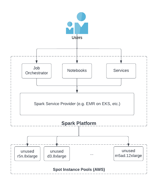
Our last SSP doesn’t provide the expected solution to these two points. They only support a limited set of Spot Instance types and by default, allow only a single Spot Instance type to be selected when launching Spark jobs. As a result, each Spark application only runs with a small capacity of Spot Instances and is vulnerable to Spot Instance terminations.
EMR on EKS uses Amazon Elastic Kubernetes Service (Amazon EKS) for accessing Spot Instances in AWS. Amazon EKS supports all available EC2 instance types, bringing a much higher capacity pool to us. We use the features of Amazon EKS managed node groups and node selectors and taints to assign each Spark application to a node group that is made of multiple instance types. After moving to EMR on EKS, we observed the following benefits:
- Spot Instance termination was less frequent and our Spark applications’ runtime became shorter and stayed stable.
- Engineers were able to iterate faster as they saw improvement in the predictability of application behaviors.
- The infrastructure costs dropped significantly because we no longer needed costly workarounds and, simultaneously, we had a sophisticated selection of instances in each node group of Amazon EKS. We were able to save approximately 50% of computing costs without the workarounds like running in multiple Availability Zones and simultaneously provide the expected level of reliability.
Smooth debugging experience
An infrastructure that supports engineers conveniently debugging the Spark application is critical to close the loop of our engineering workflow. Apache Spark uses event logs to record the activities of a Spark application, such as task start and finish. These events are formatted in JSON and are used by SHS to rerender the UI of Spark applications. Engineers can access SHS to debug task failure reasons or performance issues.
The major challenge for engineers in SafeGraph was the scalability issue in SHS. As shown in the left part of the following figure, our previous SSP forced all engineers to share the same SHS instance. As a result, SHS was under intense resource pressure due to many engineers accessing at the same time for debugging their applications, or if a Spark application had a large event log to be rendered. Prior to moving to EMR on EKS, we frequently experienced either slowness of SHS or SHS crashed completely.
As shown in the following figure, for every request to view Spark history UI, EMR on EKS starts an independent SHS instance container in an AWS-managed environment. The benefit of this architecture is two-fold:
- Different users and Spark applications won’t compete for SHS resources anymore. Therefore, we never experience slowness or crashes of SHS.
- All SHS containers are managed by AWS; users don’t need pay additional financial or operational costs to enjoy the scalable architecture.

Manageable Spark platform
As shown in the engineering workflow, building a Spark platform is not a one-off effort, and platform teams need to manage the Spark platform and keep optimizing each step in the engineer development workflow. The role of the SSP should provide the right facilities to ease operational burden as much as possible. Although there are many types of operational tasks, we focus on two of them in this post: computing resource SKU management and Spark distro version management.
Computing resource SKU management refers to the design and process for a Spark platform to allow users to choose different sizes of computing instances. Such a design and process would largely rely on the relevant functionality implemented from SSPs.
The following figure shows the SKU management with our previous SSP.

The following figure shows SKU management with EMR on EKS.

With our previous SSP, job configuration only allowed explicitly specifying a single Spot Instance type, and if that type ran out of Spot capacity, the job switched to On-Demand or fell into reliability issues. This left platform engineers with the choice of changing the settings across the fleet of Spark jobs or risking unwanted surprises for their budget and cost of goods sold.
EMR on EKS makes it much easier for the platform team to manage computing SKUs. In SafeGraph, we embedded a Spark service client between users and EMR on EKS. The Spark service client exposes only different tiers of resources to users (such as small, medium, and large). Each tier is mapped to a certain node group configured in Amazon EKS. This design brings the following benefits:
- In the case of prices and capacity changes, it’s easy for us to update configurations in node groups and keep it abstracted from users. Users don’t change anything, or even feel it, and continue to enjoy the stable resource provisioning while we keep costs and operational overhead as low as possible.
- When choosing the right resources for the Spark application, end-users don’t need to do any guess work because it’s easy to choose with simplified configuration.
Improved Spark distro release management is the other benefit we gain from EMR on EKS. Prior to using EMR on EKS, we suffered from the non-transparent release of Spark distro in our SSP. Every 1–2 months, there is a new patched version of Spark distro released to users. These versions are all exposed to users via their UI. This resulted in engineers choosing various versions of distro, some of which hadn’t been tested with our internal tools. It significantly increased the breaking rate of our pipelines, internal systems, and the support burden of platform teams. We expect that the risk from releases of Spark distros should be minimum and transparent to users with an EMR on EKS architecture.
EMR on EKS follows the best practices with a stable base Docker image containing a fixed version of Spark distro. For any change of Spark distro, we have to explicitly rebuild and roll out the Docker image. With EMR on EKS, we can keep a new version of Spark distro hidden from users before testing it with our internal toolings and systems and make a formal release.
Conclusion
In this post, we shared our journey building a Spark platform on top of EMR on EKS. EMR on EKS as the SSP serves as a strong foundation of our Spark platform. With EMR on EKS, we were able to resolve challenges ranging from dependency management, resource provisioning, and debugging experience, and also significantly reduce our computing cost by 50% due to higher availability of Spot Instance types and sizes.
We hope this post could share some insights to the community when choosing the right SSP for your business. Learn more about EMR on EKS, including benefits, features, and how to get started.
About the Authors
 Nan Zhu is the Tech Lead Manager of the platform team in SafeGraph. He leads the team to build a broad range of infrastructure and internal toolings to improve the reliability, efficiency and productivity of the SafeGraph engineering process, e.g. internal Spark ecosystem, metrics store and CI/CD for large mono repos, etc. He is also involved in multiple open source projects like Apache Spark, Apache Iceberg, Gluten, etc.
 Dave Thibault is a Sr. Solutions Architect serving AWS’s independent software vendor (ISV) customers. He’s passionate about building with serverless technologies, machine learning, and accelerating his AWS customers’ business success. Prior to joining AWS, Dave spent 17 years in life sciences companies doing IT and informatics for research, development, and clinical manufacturing groups. He also enjoys snowboarding, plein air oil painting, and spending time with his family.
Amazon Redshift is the most widely used data warehouse in the cloud, best suited for analyzing exabytes of data and running complex analytical queries. Amazon QuickSight is a fast business analytics service to build visualizations, perform ad hoc analysis, and quickly get business insights from your data. QuickSight provides easy integration with Amazon Redshift, providing native access to all your data and enabling organizations to scale their business analytics capabilities to hundreds of thousands of users. QuickSight delivers fast and responsive query performance by using a robust in-memory engine (SPICE).
As a QuickSight administrator, you can use AWS CloudFormation templates to migrate assets between distinct environments from development, to test, to production. AWS CloudFormation helps you model and set up your AWS resources so you can spend less time managing those resources and more time focusing on your applications that run in AWS. You no longer need to create data sources or analyses manually. You create a template that describes all the AWS resources that you want, and AWS CloudFormation takes care of provisioning and configuring those resources for you. In addition, with versioning, you have your previous assets, which provides the flexibility to roll back deployments if the need arises. For more details, refer to Amazon QuickSight resource type reference.
In this post, we show how to automate the deployment of a QuickSight analysis connecting to an Amazon Redshift data warehouse with a CloudFormation template.
Solution overview
Our solution consists of the following steps:
- Create a QuickSight analysis using an Amazon Redshift data source.
- Create a QuickSight template for your analysis.
- Create a CloudFormation template for your analysis using the AWS Command Line Interface (AWS CLI).
- Use the generated CloudFormation template to deploy a QuickSight analysis to a target environment.
The following diagram shows the architecture of how you can have multiple AWS accounts, each with its own QuickSight environment connected to its own Amazon Redshift data source. In this post, we outline the steps involved in migrating QuickSight assets in the dev account to the prod account. For this post, we use Amazon Redshift as the data source and create a QuickSight visualization using the Amazon Redshift sample TICKIT database.

The following diagram illustrates flow of the high-level steps.

Prerequisites
Before setting up the CloudFormation stacks, you must have an AWS account and an AWS Identity and Access Management (IAM) user with sufficient permissions to interact with the AWS Management Console and the services listed in the architecture.
The migration requires the following prerequisites:
- A QuickSight enterprise account in the source and target accounts. For instructions, see Setting up for Amazon QuickSight.
- A connection between QuickSight and the Amazon Redshift instance. For instructions, refer to Authorizing connections from Amazon QuickSight to Amazon Redshift clusters.
- An Amazon Redshift cluster with sample data loaded. For instructions, see Using a sample dataset.
- You can use AWS Cloud9 or AWS CloudShell from the console to run AWS CLI commands.
Create a QuickSight analysis in your dev environment
In this section, we walk through the steps to set up your QuickSight analysis using an Amazon Redshift data source.
Create an Amazon Redshift data source
To connect to your Amazon Redshift data warehouse, you need to create a data source in QuickSight. As shown in the following screenshot, you have two options:
- Auto-discovered
- Manual connect

QuickSight auto-discovers Amazon Redshift clusters that are associated with your AWS account. These resources must be located in the same Region as your QuickSight account.
For more details, refer to Authorizing connections from Amazon QuickSight to Amazon Redshift clusters.
You can also manually connect and create a data source.

Create an Amazon Redshift dataset
The next step is to create a QuickSight dataset, which identifies the specific data in a data source you want to use.
For this post, we use the TICKIT database created in an Amazon Redshift data warehouse, which consists of seven tables: two fact tables and five dimensions, as shown in the following figure.

This sample database application helps analysts track sales activity for the fictional TICKIT website, where users buy and sell tickets online for sporting events, shows, and concerts.
- On the Datasets page, choose New dataset.
- Choose the data source you created in the previous step.
- Choose Use custom SQL.
- Enter the custom SQL as shown in the following screenshot.
 |  |
The following screenshot shows our completed data source.

Create a QuickSight analysis
The next step is to create an analysis that utilizes this dataset. In QuickSight, you analyze and visualize your data in analyses. When you’re finished, you can publish your analysis as a dashboard to share with others in your organization.
- On the All analyses tab of the QuickSight start page, choose New analysis.

The Datasets page opens.
- Choose a dataset, then choose Use in analysis.

- Create a visual. For more information about creating visuals, see Adding visuals to Amazon QuickSight analyses.

Create a QuickSight template from your analysis
A QuickSight template is a named object in your AWS account that contains the definition of your analysis and references to the datasets used. You can create a template using the QuickSight API by providing the details of the source analysis via a parameter file. You can use templates to easily create a new analysis.
You can use AWS Cloud9 from the console to run AWS CLI commands.

The following AWS CLI command demonstrates how to create a QuickSight template based on the sales analysis you created (provide your AWS account ID for your dev account):
The parameter.json file contains the following details (provide your source QuickSight user ARN, analysis ARN, and dataset ARN):
You can use the AWS CLI describe-user, describe\_analysis, and describe\_dataset commands to get the required ARNs.
To upload the updated parameter.json file to AWS Cloud9, choose File from the tool bar and choose Upload local file.

The QuickSight template is created in the background. QuickSight templates aren’t visible within the QuickSight UI; they’re a developer-managed or admin-managed asset that is only accessible via the AWS CLI or APIs.
To check the status of the template, run the describe-template command:
The following code shows command output:

Copy the template ARN; we need it later to create a template in the production account.
The QuickSight template permissions in the dev account need to be updated to give access to the prod account. Run the following command to update the QuickSight template. This provides the describe privilege to the target account to extract details of the template from the source account:
The file TemplatePermission.json contains the following details (provide your target AWS account ID):
To upload the updated TemplatePermission.json file to AWS Cloud9, choose the File menu from the tool bar and choose Upload local file.
Create a CloudFormation template
In this section, we create a CloudFormation template containing our QuickSight assets. In this example, we use a YAML formatted template saved on our local machine. We update the following different sections of the template:
- AWS::QuickSight::DataSource
- AWS::QuickSight::DataSet
- AWS::QuickSight::Template
- AWS::QuickSight::Analysis
Some of the information required to complete the CloudFormation template can be gathered from the source QuickSight account via the describe AWS CLI commands, and some information needs to be updated for the target account.
Create an Amazon Redshift data source in AWS CloudFormation
In this step, we add the AWS::QuickSight::DataSource section of the CloudFormation template.
Gather the following information on the Amazon Redshift cluster in the target AWS account (production environment):
- VPC connection ARN
- Host
- Port
- Database
- User
- Password
- Cluster ID
You have the option to create a custom DataSourceID. This ID is unique per Region for each AWS account.
Add the following information to the template:
Create an Amazon Redshift dataset in AWS CloudFormation
In this step, we add the AWS::QuickSight::DataSet section in the CloudFormation template to match the dataset definition from the source account.
Gather the dataset details and run the list-data-sets command to get all datasets from the source account (provide your source dev account ID):
The following code is the output:

Run the describe-data-set command, specifying the dataset ID from the previous command’s response:
The following code shows partial output:

Based on the dataset description, add the AWS::Quicksight::DataSet resource in the CloudFormation template, as shown in the following code. Note that you can also create a custom DataSetID. This ID is unique per Region for each AWS account.
You can specify ImportMode to choose between Direct\_Query or Spice.
Create a QuickSight template in AWS CloudFormation
In this step, we add the AWS::QuickSight::Template section in the CloudFormation template, representing the analysis template.
Use the source template ARN you created earlier and add the AWS::Quicksight::Template resource in the CloudFormation template:
Create a QuickSight analysis
In this last step, we add the AWS::QuickSight::Analysis section in the CloudFormation template. The analysis is linked to the template created in the target account.
Add the AWS::Quicksight::Analysis resource in the CloudFormation template as shown in the following code:
Deploy the CloudFormation template in the production account
To create a new CloudFormation stack that uses the preceding template via the AWS CloudFormation console, complete the following steps:
- On the AWS CloudFormation console, choose Create Stack.
- On the drop-down menu, choose with new resources (standard).
- For Prepare template, select Template is ready.
- For Specify template, choose Upload a template file.
- Save the provided CloudFormation template in a .yaml file and upload it.
- Choose Next.
- Enter a name for the stack. For this post, we use
QS-RS-CF-Stack. - Choose Next.
- Choose Next again.
- Choose Create Stack.

The status of the stack changes to CREATE\_IN\_PROGRESS, then to CREATE\_COMPLETE.

Verify the QuickSight objects in the following table have been created in the production environment.
| QuickSight Object Type | Object Name (Dev) | Object Name ( Prod) |
| Data Source | RS-Sales-DW | RS-Sales-DW |
| Dataset | Sales | Sales |
| Template | QS-RS-Sales-Temp | QS-RS-SalesAnalysis-Temp |
| Analysis | Sales Analysis | Sales-Analysis |
The following example shows that Sales Analysis was created in the target account.

Conclusion
This post demonstrated an approach to migrate a QuickSight analysis with an Amazon Redshift data source from one QuickSight account to another with a CloudFormation template.
For more information about automating dashboard deployment, customizing access to the QuickSight console, configuring for team collaboration, and implementing multi-tenancy and client user segregation, check out the videos Virtual Admin Workshop: Working with Amazon QuickSight APIs and Admin Level-Up Virtual Workshop, V2 on YouTube.
About the author
Sandeep Bajwa is a Sr. Analytics Specialist based out of Northern Virginia, specialized in the design and implementation of analytics and data lake solutions.
Amazon EMR Serverless is a serverless option in Amazon EMR that makes it simple to run applications using open-source analytics frameworks such as Apache Spark and Hive without configuring, managing, or scaling clusters.
At AWS re:Invent 2022, we announced support for running serverless Spark and Hive workloads with AWS Graviton2 (Arm64) on Amazon EMR Serverless. AWS Graviton2 processors are custom-built by AWS using 64-bit Arm Neoverse cores, delivering a significant leap in price-performance for your cloud workloads.
This post discusses the performance improvements observed while running Apache Spark jobs using AWS Graviton2 on EMR Serverless. We found that Graviton2 on EMR Serverless achieved 10% performance improvement for Spark workloads based on runtime. AWS Graviton2 is offered at a 20% lower cost than the x86 architecture option (see the Amazon EMR pricing page for details), resulting in a 27% overall better price-performance for workloads.
Spark performance test results
The following charts compare the benchmark runtime with and without Graviton2 for a EMR Serverless Spark application (note that the charts are not drawn to scale). We observed up to 10% improvement in total runtime and 8% improvement in geometric mean for the queries compared to x86.


The following table summarizes our results.
| Metric | Graviton2 | x86 | %Gain |
| Total Execution Time (in seconds) | 2,670 | 2,959 | 10% |
| Geometric Mean (in seconds) | 22.06 | 24.07 | 8% |
Testing configuration
To evaluate the performance improvements, we use benchmark tests derived from TPC-DS 3 TB scale performance benchmarks. The benchmark consists of 104 queries, and each query is submitted sequentially to an EMR Serverless application. EMR Serverless has automatic and fine-grained scaling enabled by default. Spark provides Dynamic Resource Allocation (DRA) to dynamically adjust the application resources based on the workload, and EMR Serverless uses the signals from DRA to elastically scale workers as needed. For our tests, we chose a predefined pre-initialized capacity that allows the application to scale to default limits. Each application has 1 driver and 100 workers configured as pre-initialized capacity, allowing it to scale to a maximum of 8000 vCPU/60000 GB capacity. When launching the applications, as default we use x86\_64 to get baseline numbers and Arm64 for AWS Graviton2, and the application had VPC networking enabled.
The following table summarizes the Spark application configuration.
| Number of Drivers | Driver Size | Number of Executors | Executor Size | Ephemeral Storage | Amazon EMR release label |
| 1 | 4 vCPUs, 16 GB Memory | 100 | 4 vCPUs, 16 GB Memory | 200 G | 6.9 |
Performance test results and cost comparison
Let’s do a cost comparison of the benchmark tests. Because we used 1 driver [4 vCPUs, 16 GB memory] and 100 executors [4 vCPUs, 16 GB memory] for each run, the total capacity used is 4*101=192 vCPUs, 16*101=1616 GB memory, 200*100=20000 GB storage. The following table summarizes the cost.
| Test | Total time (Seconds) | vCPUs | Memory (GB) | Ephemeral (Storage GB) | Cost |
| x86\_64 | 2,958.82 | 404 | 1616 | 18000 | $26.73 |
| Graviton2 | 2,670.38 | 404 | 1616 | 18000 | $19.59 |
The calculations are as follows:
- Total vCPU cost = (number of vCPU * per vCPU rate * job runtime in hour)
- Total GB = (Total GB of memory configured * per GB-hours rate * job runtime in hour)
- Storage = 20 GB of ephemeral storage is available for all workers by default—you pay only for any additional storage that you configure per worker
Cost breakdown
Let’s look at the cost breakdown for x86:
- Job runtime – 49.3 minutes = 0.82 hours
- Total vCPU cost – 404 vCPUs x 0.82 hours job runtime x 0.052624 USD per vCPU = 17.4333 USD
- Total GB cost – 1,616 memory-GBs x 0.82 hours job runtime x 0.0057785 USD per memory GB = 7.6572 USD
- Storage cost – 18,000 storage-GBs x 0.82 hours job runtime x 0.000111 USD per storage GB = 1.6386 USD
- Additional storage – 20,000 GB – 20 GB free tier * 100 workers = 18,000 additional storage GB
- EMR Serverless total cost (x86): 17.4333 USD + 7.6572 USD + 1.6386 USD = 26.7291 USD
Let’s compare to the cost breakdown for Graviton 2:
- Job runtime – 44.5 minutes = 0.74 hours
- Total vCPU cost – 404 vCPUs x 0.74 hours job runtime x 0.042094 USD per vCPU = 12.5844 USD
- Total GB cost – 1,616 memory-GBs x 0.74 hours job runtime x 0.004628 USD per memory GB = 5.5343 USD
- Storage cost – 18,000 storage-GBs x 0.74 hours job runtime x 0.000111 USD per storage GB = 1.4785 USD
- Additional storage – 20,000 GB – 20 GB free tier * 100 workers = 18,000 additional storage GB
- EMR Serverless total cost (Graviton2): 12.5844 USD + 5.5343 USD + 1.4785 USD = 19.5972 USD
The tests indicate that for the benchmark run, AWS Graviton2 lead to an overall cost savings of 27%.
Individual query improvements and observations
The following chart shows the relative speedup of individual queries with Graviton2 compared to x86.

We see some regression in a few shorter queries, which had little impact on the overall benchmark runtime. We observed better performance gains for long running queries, for example:
- q67 average 86 seconds for x86, 74 seconds for Graviton2 with 24% runtime performance gain
- q23a and q23b gained 14% and 16%, respectively
- q32 regressed by 7%; the difference between average runtime is <500 milliseconds (11.09 seconds for Graviton2 vs. 10.39 seconds for x86)
To quantify performance, we use benchmark SQL derived from TPC-DS 3 TB scale performance benchmarks.
If you’re evaluating migrating your workloads to Graviton2 architecture on EMR Serverless, we recommend testing the Spark workloads based on your real-world use cases. The outcome might vary based on the pre-initialized capacity and number of workers chosen. If you want to run workloads across multiple processor architectures, (for example, test the performance on x86 and Arm vCPUs) follow the walkthrough in the GitHub repo to get started with some concrete ideas.
Conclusion
As demonstrated in this post, Graviton2 on EMR Serverless applications consistently yielded better performance for Spark workloads. Graviton2 is available in all Regions where EMR Serverless is available. To see a list of Regions where EMR Serverless is available, see the EMR Serverless FAQs. To learn more, visit the Amazon EMR Serverless User Guide and sample codes with Apache Spark and Apache Hive.
If you’re wondering how much performance gain you can achieve with your use case, try out the steps outlined in this post and replace with your queries.
To launch your first Spark or Hive application using a Graviton2-based architecture on EMR Serverless, see Getting started with Amazon EMR Serverless.
About the authors
 Karthik Prabhakar is a Senior Big Data Solutions Architect for Amazon EMR at AWS. He is an experienced analytics engineer working with AWS customers to provide best practices and technical advice in order to assist their success in their data journey.
 Nithish Kumar Murcherla is a Senior Systems Development Engineer on the Amazon EMR Serverless team. He is passionate about distributed computing, containers, and everything and anything about the data.
Amazon EMR Serverless allows you to run open-source big data frameworks such as Apache Spark and Apache Hive without managing clusters and servers. With EMR Serverless, you can run analytics workloads at any scale with automatic scaling that resizes resources in seconds to meet changing data volumes and processing requirements. EMR Serverless automatically scales resources up and down to provide just the right amount of capacity for your application.
We are excited to announce that EMR Serverless now offers worker configurations of 8 vCPUs with up to 60 GB memory and 16 vCPUs with up to 120 GB memory, allowing you to run more compute and memory-intensive workloads on EMR Serverless. An EMR Serverless application internally uses workers to execute workloads. and you can configure different worker configurations based on your workload requirements. Previously, the largest worker configuration available on EMR Serverless was 4 vCPUs with up to 30 GB memory. This capability is especially beneficial for the following common scenarios:
- Shuffle-heavy workloads
- Memory-intensive workloads
Let’s look at each of these use cases and the benefits of having larger worker sizes.
Benefits of using large workers for shuffle-intensive workloads
In Spark and Hive, shuffle occurs when data needs to be redistributed across the cluster during a computation. When your application performs wide transformations or reduce operations such as join, groupBy, sortBy, or repartition, Spark and Hive triggers a shuffle. Also, every Spark stage and Tez vertex is bounded by a shuffle operation. Taking Spark as an example, by default, there are 200 partitions for every Spark job defined by spark.sql.shuffle.partitions. However, Spark will compute the number of tasks on the fly based on the data size and the operation being performed. When a wide transformation is performed on top of a large dataset, there could be GBs or even TBs of data that need to be fetched by all the tasks.
Shuffles are typically expensive in terms of both time and resources, and can lead to performance bottlenecks. Therefore, optimizing shuffles can have a significant impact on the performance and cost of a Spark job. With large workers, more data can be allocated to each executor’s memory, which minimizes the data shuffled across executors. This in turn leads to increased shuffle read performance because more data will be fetched locally from the same worker and less data will be fetched remotely from other workers.
Experiments
To demonstrate the benefits of using large workers for shuffle-intensive queries, let’s use q78 from TPC-DS, which is a shuffle-heavy Spark query that shuffles 167 GB of data over 12 Spark stages. Let’s perform two iterations of the same query with different configurations.
The configurations for Test 1 are as follows:
- Size of executor requested while creating EMR Serverless application = 4 vCPUs, 8 GB memory, 200 GB disk
- Spark job config:
spark.executor.cores= 4spark.executor.memory= 8spark.executor.instances= 48- Parallelism = 192 (
spark.executor.instances*spark.executor.cores)
The configurations for Test 2 are as follows:
- Size of executor requested while creating EMR Serverless application = 8 vCPUs, 16 GB memory, 200 GB disk
- Spark job config:
spark.executor.cores= 8spark.executor.memory= 16spark.executor.instances= 24- Parallelism = 192 (
spark.executor.instances*spark.executor.cores)
Let’s also disable dynamic allocation by setting spark.dynamicAllocation.enabled to false for both tests to avoid any potential noise due to variable executor launch times and keep the resource utilization consistent for both tests. We use Spark Measure, which is an open-source tool that simplifies the collection and analysis of Spark performance metrics. Because we’re using a fixed number of executors, the total number of vCPUs and memory requested are the same for both the tests. The following table summarizes the observations from the metrics collected with Spark Measure.
| . | Total Time Taken for Query in milliseconds | shuffleLocalBlocksFetched | shuffleRemoteBlocksFetched | shuffleLocalBytesRead | shuffleRemoteBytesRead | shuffleFetchWaitTime | shuffleWriteTime |
| Test 1 | 153244 | 114175 | 5291825 | 3.5 GB | 163.1 GB | 1.9 hr | 4.7 min |
| Test 2 | 108136 | 225448 | 5185552 | 6.9 GB | 159.7 GB | 3.2 min | 5.2 min |
As seen from the table, there is a significant difference in performance due to shuffle improvements. Test 2, with half the number of executors that are twice as large as Test 1, ran 29.44% faster, with 1.97 times more shuffle data fetched locally compared to Test 1 for the same query, same parallelism, and same aggregate vCPU and memory resources. Therefore, you can benefit from improved performance without compromising on cost or job parallelism with the help of large executors. We have observed similar performance benefits for other shuffle-intensive TPC-DS queries such as q23a and q23b.
Recommendations
To determine if the large workers will benefit your shuffle-intensive Spark applications, consider the following:
- Check the Stages tab from the Spark History Server UI of your EMR Serverless application. For example, from the following screenshot of Spark History Server, we can determine that this Spark job wrote and read 167 GB of shuffle data aggregated across 12 stages, looking at the Shuffle Read and Shuffle Write columns. If your jobs shuffle over 50 GB of data, you may potentially benefit from using larger workers with 8 or 16 vCPUs or
spark.executor.cores.

- Check the SQL / DataFrame tab from the Spark History Server UI of your EMR Serverless application (only for Dataframe and Dataset APIs). When you choose the Spark action performed, such as collect, take, showString, or save, you will see an aggregated DAG for all stages separated by the exchanges. Every exchange in the DAG corresponds to a shuffle operation, and it will contain the local and remote bytes and blocks shuffled, as seen in the following screenshot. If the local shuffle blocks or bytes fetched is much less compared to the remote blocks or bytes fetched, you can rerun your application with larger workers (with 8 or 16 vCPUs or spark.executor.cores) and review these exchange metrics in a DAG to see if there is any improvement.
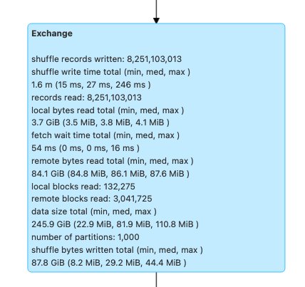
- Use the Spark Measure tool with your Spark query to obtain the shuffle metrics in the Spark driver’s
stdoutlogs, as shown in the following log for a Spark job. Review the time taken for shuffle reads (shuffleFetchWaitTime) and shuffle writes (shuffleWriteTime), and the ratio of the local bytes fetched to the remote bytes fetched. If the shuffle operation takes more than 2 minutes, rerun your application with larger workers (with 8 or 16 vCPUs orspark.executor.cores) with Spark Measure to track the improvement in shuffle performance and the overall job runtime.
Benefits of using large workers for memory-intensive workloads
Certain types of workloads are memory-intensive and may benefit from more memory configured per worker. In this section, we discuss common scenarios where large workers could be beneficial for running memory-intensive workloads.
Data skew
Data skews commonly occur in several types of datasets. Some common examples are fraud detection, population analysis, and income distribution. For example, when you want to detect anomalies in your data, it’s expected that only less than 1% of the data is abnormal. If you want to perform some aggregation on top of normal vs. abnormal records, 99% of the data will be processed by a single worker, which may lead to that worker running out of memory. Data skews may be observed for memory-intensive transformations like groupBy, orderBy, join, window functions, collect\_list, collect\_set, and so on. Join types such as BroadcastNestedLoopJoin and Cartesan product are also inherently memory-intensive and susceptible to data skews. Similarly, if your input data is Gzip compressed, a single Gzip file can’t be read by more than one task because the Gzip compression type is unsplittable. When there are a few very large Gzip files in the input, your job may run out of memory because a single task may have to read a huge Gzip file that doesn’t fit in the executor memory.
Failures due to data skew can be mitigated by applying strategies such as salting. However, this often requires extensive changes to the code, which may not be feasible for a production workload that failed due to an unprecedented data skew caused by a sudden surge in incoming data volume. For a simpler workaround, you may just want to increase the worker memory. Using larger workers with more spark.executor.memory allows you to handle data skew without making any changes to your application code.
Caching
In order to improve performance, Spark allows you to cache the data frames, datasets, and RDDs in memory. This enables you to reuse a data frame multiple times in your application without having to recompute it. By default, up to 50% of your executor’s JVM is used to cache the data frames based on the property spark.memory.storageFraction. For example, if your spark.executor.memory is set to 30 GB, then 15 GB is used for cache storage that is immune to eviction.
The default storage level of cache operation is DISK\_AND\_MEMORY. If the size of the data frame you are trying to cache doesn’t fit in the executor’s memory, a portion of the cache spills to disk. If there isn’t enough space to write the cached data in disk, the blocks are evicted and you don’t get the benefits of caching. Using larger workers allows you to cache more data in memory, boosting job performance by retrieving cached blocks from memory rather than the underlying storage.
Experiments
For example, the following PySpark job leads to a skew, with one executor processing 99.95% of the data with memory-intensive aggregates like collect\_list. The job also caches a very large data frame (2.2 TB). Let’s run two iterations of the same job on EMR Serverless with the following vCPU and memory configurations.
Let’s run Test 3 with the previously largest possible worker configurations:
- Size of executor set while creating EMR Serverless application = 4 vCPUs, 30 GB memory, 200 GB disk
- Spark job config:
spark.executor.cores= 4spark.executor.memory= 27 G
Let’s run Test 4 with the newly released large worker configurations:
- Size of executor set in while creating EMR Serverless application = 8 vCPUs, 60 GB memory, 200 GB disk
- Spark job config:
spark.executor.cores= 8spark.executor.memory= 54 G
Test 3 failed with FetchFailedException, which resulted due to the executor memory not being sufficient for the job.

Also, from the Spark UI of Test 3, we see that the reserved storage memory of the executors was fully utilized for caching the data frames.
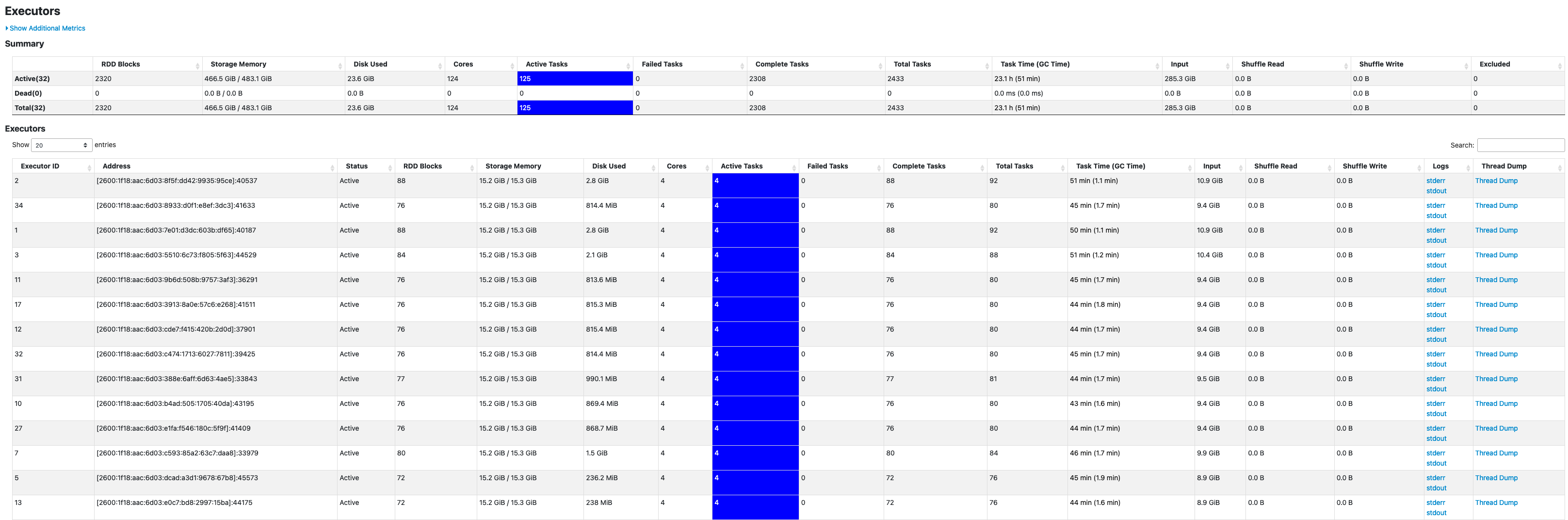
The remaining blocks to cache were spilled to disk, as seen in the executor’s stderr logs:
Around 33% of the persisted data frame was cached on disk, as seen on the Storage tab of the Spark UI.

Test 4 with larger executors and vCores ran successfully without throwing any memory-related errors. Also, only about 2.2% of the data frame was cached to disk. Therefore, cached blocks of a data frame will be retrieved from memory rather than from disk, offering better performance.

Recommendations
To determine if the large workers will benefit your memory-intensive Spark applications, consider the following:
- Determine if your Spark application has any data skews by looking at the Spark UI. The following screenshot of the Spark UI shows an example data skew scenario where one task processes most of the data (145.2 GB), looking at the Shuffle Read size. If one or fewer tasks process significantly more data than other tasks, rerun your application with larger workers with 60–120 G of memory (
spark.executor.memoryset anywhere from 54–109 GB factoring in 10% ofspark.executor.memoryOverhead).

- Check the Storage tab of the Spark History Server to review the ratio of data cached in memory to disk from the Size in memory and Size in disk columns. If more than 10% of your data is cached to disk, rerun your application with larger workers to increase the amount of data cached in memory.
- Another way to preemptively determine if your job needs more memory is by monitoring Peak JVM Memory on the Spark UI Executors tab. If the peak JVM memory used is close to the executor or driver memory, you can create an application with a larger worker and configure a higher value for
spark.executor.memoryorspark.driver.memory. For example, in the following screenshot, the maximum value of peak JVM memory usage is 26 GB andspark.executor.memoryis set to 27 G. In this case, it may be beneficial to use larger workers with 60 GB memory andspark.executor.memoryset to 54 G.

Considerations
Although large vCPUs help increase the locality of the shuffle blocks, there are other factors involved such as disk throughput, disk IOPS (input/output operations per second), and network bandwidth. In some cases, more small workers with more disks could offer higher disk IOPS, throughput, and network bandwidth overall compared to fewer large workers. We encourage you to benchmark your workloads against suitable vCPU configurations to choose the best configuration for your workload.
For shuffle-heavy jobs, it’s recommended to use large disks. You can attach up to 200 GB disk to each worker when you create your application. Using large vCPUs (spark.executor.cores) per executor may increase the disk utilization on each worker. If your application fails with “No space left on device” due to the inability to fit shuffle data in the disk, use more smaller workers with 200 GB disk.
Conclusion
In this post, you learned about the benefits of using large executors for your EMR Serverless jobs. For more information about different worker configurations, refer to Worker configurations. Large worker configurations are available in all Regions where EMR Serverless is available.
About the Author
 Veena Vasudevan is a Senior Partner Solutions Architect and an Amazon EMR specialist at AWS focusing on big data and analytics. She helps customers and partners build highly optimized, scalable, and secure solutions; modernize their architectures; and migrate their big data workloads to AWS.
This is a guest post co-written with Frank Contrepois from Strategic Blue.
For over 10 years, Strategic Blue has helped organizations unlock the most value from the cloud by enabling their customers to purchase non-standard commitments. By taking a commodity trading approach to purchasing from AWS, Strategic Blue helps customers purchase commitments for varying lengths of time, such as a 9-month Reserved Instance or an 18-month Savings Plan. Over the years, they’ve been able to help customers save millions by maximizing commitments.
In this post, we share how Strategic Blue uses Amazon QuickSight and AWS Cost and Usage Reports to help their customers save costs.
The challenge
Buying and selling AWS differently means that the cost and usage data available to Strategic Blue on the AWS Management Console only matches what they purchased—not what their customers purchased. In order to accurately bill their customers, Strategic Blue has built a billing system that takes AWS Cost and Usage Reports (CUR) as input and outputs a pro forma CUR that matches what their customers would expect to see. Although the CUR remains a critical source of data, it can have hundreds of columns and millions of rows, making it very difficult for Strategic Blue’s customers to visualize and understand.
Initially, in order to give their customers a way to visualize and understand their spend, Strategic Blue started building a dashboard from scratch using QuickSight, AWS Glue, and Amazon Athena. The idea was to build a dashboard accessible to all of Strategic Blue’s customers (as soon as they were onboarded) that enabled them to see their true cost and usage. QuickSight provides modern interactive dashboards that enable fast time-to-insights and have features that allow for the easy embedding of dashboards into web applications linked to a customer’s single sign-on (SSO) solution. Combined with row-level-security, a dashboard can be pre-filtered to show an individual user’s cost and usage information for only the accounts they are responsible for.
However, figuring out how to accurately show cost and usage insights from the CUR from scratch was a challenge. The amount of work required to decode the raw content of the CUR to build something that matches what you would see in AWS Cost Explorer quickly became overwhelming.
The solution
To help you visualize the treasure trove of data available in a CUR file, AWS created the Cloud Intelligence Dashboards solution. The Cloud Intelligence Dashboards provide a full stack of capabilities, deployed via AWS CloudFormation or other methods, that include six different QuickSight dashboards geared towards helping you optimize your spend on AWS.
Strategic Blue deployed the CUDOS Dashboard (one of the six dashboards available as of this writing) to solve their business case for providing their customers with accurate, comprehensive insights into their cost and usage.
“The Cloud Intelligence Dashboards provided all of the accurate CUR calculations and maintenance we need. This saves us many hours of reverse engineering to keep pace with AWS innovation and changes as their product and billing mechanisms mature.”
– Frank Contrepois, Head of FinOps at Strategic Blue.
The following screenshot shows an example of the dashboard.

Embedding and scaling to all customers
Strategic Blue uses the embedding and row-level security features of QuickSight to scale the dashboards to every customer the moment they are onboarded. By integrating their SSO Amazon Cognito with QuickSight, Strategic Blue is able to provide customers instant access to an instance of CUDOS through a portal as soon as they are onboarded to Strategic Blue’s platform. The row-level security setup managed by administrators within Strategic Blue makes sure that their customers only ever see their own cost and usage data. This helps Strategic Blue offer the protection and security customers expect.
To see the Strategic Blue portal with embedded CUDOS in action, watch the following demo video, or to unlock your savings potential in the cloud, sign up with Strategic Blue now.
Now that CUDOS is embedded into Strategic Blue’s portal, they are able to offer additional value free of charge to their customers. Strategic Blue’s portal uses the customer’s CUDOS dashboard to find opportunities to save and optimize. After the engagement, Strategic Blue will continue to analyze the impact of their customer’s cost optimization measures, reporting back to them what they’ve saved and what additional opportunities there are to further optimize.
Strategic Blue is already seeing an impact. Since enabling an embedded version of CUDOS for every customer and for internal teams, Strategic Blue is seeing a 27% increase in positive feedback for regular meetings, 31% fewer support tickets related to questions about cost, and a move from tactical to strategic FinOps conversations.
The future
Strategic Blue plans to evaluate and embed the rest of the Cloud Intelligence Dashboards, such as the KPI Dashboard to help customers track goals and metrics around cost optimization, and the Trusted Advisor Organizational Dashboard, which helps customers stay on top of underutilized resources as well as operational information such as security and fault tolerance postures. With the foundation in place and QuickSight’s ease of use, Strategic Blue will continue working closely with customers to customize and refine the dashboards to meet specific customer needs, improving and expanding their offerings.
Conclusion
In this post, we covered how Strategic Blue used Cloud Intelligence Dashboards built on QuickSight to help customers get accurate insights into their cloud cost and usage. Strategic Blue’s customers can access stunning and interactive dashboards that can be customized with ease and without the need for technical skills. The comprehensive embedding capabilities, granular row-level-security, and SSO integrations of QuickSight ensure that Strategic Blue is able to provide customers secure and seamless access to their Cloud Intelligence Dashboards.
It’s easy to install Cloud Intelligence Dashboards in your account. Visit Cloud Intelligence Dashboards for details on how to deploy the dashboards today, and let us know how it goes.
About the Authors
 Frank Contrepois is the Head of FinOps at Strategic Blue. Frank and his team support a wide range of customers to implement Cloud FinOps including small-and medium-sized organizations, private equity (PE) funds and investors, enterprises and global cloud resellers striking significant deals. He is an AWS APN Ambassador and has several AWS and GCP pro-level certifications. Outside of work, he is a husband, father of two wonderful boys, and co-host of the “What’s new with in Cloud FinOps” podcast.
 Aaron Edell is Head of GTM for Customer Cloud Intelligence for Amazon Web Services. He is responsible for building and scaling businesses around Cloud Financial Management, FinOps, and the Well-Architected Cost Optimization pillar. He focuses his GTM efforts on the Cloud Intelligence Dashboards and remains obsessed with helping all customers get better visibility and access to their cost and usage data.
Organizations have chosen to build data lakes on top of Amazon Simple Storage Service (Amazon S3) for many years. A data lake is the most popular choice for organizations to store all their organizational data generated by different teams, across business domains, from all different formats, and even over history. According to a study, the average company is seeing the volume of their data growing at a rate that exceeds 50% per year, usually managing an average of 33 unique data sources for analysis.
Teams often try to replicate thousands of jobs from relational databases with the same extract, transform, and load (ETL) pattern. There is lot of effort in maintaining the job states and scheduling these individual jobs. This approach helps the teams add tables with few changes and also maintains the job status with minimum effort. This can lead to a huge improvement in the development timeline and tracking the jobs with ease.
In this post, we show you how to easily replicate all your relational data stores into a transactional data lake in an automated fashion with a single ETL job using Apache Iceberg and AWS Glue.
Solution architecture
Data lakes are usually organized using separate S3 buckets for three layers of data: the raw layer containing data in its original form, the stage layer containing intermediate processed data optimized for consumption, and the analytics layer containing aggregated data for specific use cases. In the raw layer, tables usually are organized based on their data sources, whereas tables in the stage layer are organized based on the business domains they belong to.
This post provides an AWS CloudFormation template that deploys an AWS Glue job that reads an Amazon S3 path for one data source of the data lake raw layer, and ingests the data into Apache Iceberg tables on the stage layer using AWS Glue support for data lake frameworks. The job expects tables in the raw layer to be structured in the way AWS Database Migration Service (AWS DMS) ingests them: schema, then table, then data files.
This solution uses AWS Systems Manager Parameter Store for table configuration. You should modify this parameter specifying the tables you want to process and how, including information such as primary key, partitions, and the business domain associated. The job uses this information to automatically create a database (if it doesn’t already exist) for every business domain, create the Iceberg tables, and perform the data loading.
Finally, we can use Amazon Athena to query the data in the Iceberg tables.
The following diagram illustrates this architecture.

This implementation has the following considerations:
- All tables from the data source must have a primary key to be replicated using this solution. The primary key can be a single column or a composite key with more than one column.
- If the data lake contains tables that don’t need upserts or don’t have a primary key, you can exclude them from the parameter configuration and implement traditional ETL processes to ingest them into the data lake. That’s outside of the scope of this post.
- If there are additional data sources that need to be ingested, you can deploy multiple CloudFormation stacks, one to handle each data source.
- The AWS Glue job is designed to process data in two phases: the initial load that runs after AWS DMS finishes the full load task, and the incremental load that runs on a schedule that applies change data capture (CDC) files captured by AWS DMS. Incremental processing is performed using an AWS Glue job bookmark.
There are nine steps to complete this tutorial:
- Set up a source endpoint for AWS DMS.
- Deploy the solution using AWS CloudFormation.
- Review the AWS DMS replication task.
- Optionally, add permissions for encryption and decryption or AWS Lake Formation.
- Review the table configuration on Parameter Store.
- Perform initial data loading.
- Perform incremental data loading.
- Monitor table ingestion.
- Schedule incremental batch data loading.
Prerequisites
Before starting this tutorial, you should already be familiar with Iceberg. If you’re not, you can get started by replicating a single table following the instructions in Implement a CDC-based UPSERT in a data lake using Apache Iceberg and AWS Glue. Additionally, set up the following:
- Two S3 buckets for data lake layers: raw and stage. You can reuse existing ones.
- An S3 bucket for AWS Glue scripts, temporary data, and logs.
- An existing relational database instance with tables with data. If you don’t have one, you can deploy a PostgreSQL instance on Amazon Relational Database Service (Amazon RDS). For instructions, refer to Create and Connect to a PostgreSQL Database with Amazon RDS. To populate the data, you can follow instructions to use a simple NFL database on the AWS Samples GitHub.
- An AWS DMS replication instance, if you don’t have one running. For instructions, refer to How do I create an AWS DMS replication instance.
- An AWS Identity and Access Management (IAM) role for AWS DMS to write data into Amazon S3. The role must have permissions to write into the bucket designated for the raw layer of the data lake. For instructions to set up these permissions, refer to Prerequisites for using Amazon S3 as a target.
Set up a source endpoint for AWS DMS
Before we create our AWS DMS task, we need to set up a source endpoint to connect to the source database:
- On the AWS DMS console, choose Endpoints in the navigation pane.
- Choose Create endpoint.
- If your database is running on Amazon RDS, choose Select RDS DB instance, then choose the instance from the list. Otherwise, choose the source engine and provide the connection information either through AWS Secrets Manager or manually.
- For Endpoint identifier, enter a name for the endpoint; for example, source-postgresql.
- Choose Create endpoint.
Deploy the solution using AWS CloudFormation
Create a CloudFormation stack using the provided template. Complete the following steps:
- Choose Launch Stack:
- Choose Next.
- Provide a stack name, such as
transactionaldl-postgresql. - Enter the required parameters:
- DMSS3EndpointIAMRoleARN – The IAM role ARN for AWS DMS to write data into Amazon S3.
- ReplicationInstanceArn – The AWS DMS replication instance ARN.
- S3BucketStage – The name of the existing bucket used for the stage layer of the data lake.
- S3BucketGlue – The name of the existing S3 bucket for storing AWS Glue scripts.
- S3BucketRaw – The name of the existing bucket used for the raw layer of the data lake.
- SourceEndpointArn – The AWS DMS endpoint ARN that you created earlier.
- SourceName – The arbitrary identifier of the data source to replicate (for example,
postgres). This is used to define the S3 path of the data lake (raw layer) where data will be stored.
- Do not modify the following parameters:
- SourceS3BucketBlog – The bucket name where the provided AWS Glue script is stored.
- SourceS3BucketPrefix – The bucket prefix name where the provided AWS Glue script is stored.
- Choose Next twice.
- Select I acknowledge that AWS CloudFormation might create IAM resources with custom names.
- Choose Create stack.
After approximately 5 minutes, the CloudFormation stack is deployed.
Review the AWS DMS replication task
The AWS CloudFormation deployment created an AWS DMS target endpoint for you. Because of two specific endpoint settings, the data will be ingested as we need it on Amazon S3.
- On the AWS DMS console, choose Endpoints in the navigation pane.
- Search for and choose the endpoint that begins with
dmsIcebergs3endpoint. - Review the endpoint settings:
DataFormatis specified asparquet.TimestampColumnNamewill add the columnlast\_update\_timewith the date of creation of the records on Amazon S3.

The deployment also creates an AWS DMS replication task that begins with dmsicebergtask.
- Choose Replication tasks in the navigation pane and search for the task.
You will see that the Task Type is marked as Full load, ongoing replication. AWS DMS will perform an initial full load of existing data, and then create incremental files with changes performed to the source database.
On the Mapping Rules tab, there are two types of rules:
- A selection rule with the name of the source schema and tables that will be ingested from the source database. By default, it uses the sample database provided in the prerequisites,
dms\_sample, and all tables with the keyword %. - Two transformation rules that include in the target files on Amazon S3 the schema name and table name as columns. This is used by our AWS Glue job to know to which tables the files in the data lake correspond.
To learn more about how to customize this for your own data sources, refer to Selection rules and actions.

Let’s change some configurations to finish our task preparation.
- On the Actions menu, choose Modify.
- In the Task Settings section, under Stop task after full load completes, choose Stop after applying cached changes.
This way, we can control the initial load and incremental file generation as two different steps. We use this two-step approach to run the AWS Glue job once per each step.
- Under Task logs, choose Turn on CloudWatch logs.
- Choose Save.
- Wait about 1 minute for the database migration task status to show as Ready.
Add permissions for encryption and decryption or Lake Formation
Optionally, you can add permissions for encryption and decryption or Lake Formation.
Add encryption and decryption permissions
If your S3 buckets used for the raw and stage layers are encrypted using AWS Key Management Service (AWS KMS) customer managed keys, you need to add permissions to allow the AWS Glue job to access the data:
- For AWS KMS with IAM policies, refer to Allow a user to encrypt and decrypt with specific KMS keys to understand how to change the IAM policy
GlueJobPolicywith proper permissions - For AWS KMS with key policies, refer to Allow key users to use the KMS key to understand how to modify the KMS policy to allow the IAM role
GlueJobRoleto use it
Add Lake Formation permissions
If you’re managing permissions using Lake Formation, you need to allow your AWS Glue job to create your domain’s databases and tables through the IAM role GlueJobRole.
- Grant permissions to create databases (for instructions, refer to Creating a Database).
- Grant SUPER permissions to the
defaultdatabase. - Grant data location permissions.
- If you create databases manually, grant permissions on all databases to create tables. Refer to Granting table permissions using the Lake Formation console and the named resource method or Granting Data Catalog permissions using the LF-TBAC method according to your use case.
After you complete the later step of performing the initial data load, make sure to also add permissions for consumers to query the tables. The job role will become the owner of all the tables created, and the data lake admin can then perform grants to additional users.
Review table configuration in Parameter Store
The AWS Glue job that performs the data ingestion into Iceberg tables uses the table specification provided in Parameter Store. Complete the following steps to review the parameter store that was configured automatically for you. If needed, modify according to your own needs.
- On the Parameter Store console, choose My parameters in the navigation pane.
The CloudFormation stack created two parameters:
iceberg-configfor job configurationsiceberg-tablesfor table configuration
- Choose the parameter iceberg-tables.
The JSON structure contains information that AWS Glue uses to read data and write the Iceberg tables on the target domain:
- One object per table – The name of the object is created using the schema name, a period, and the table name; for example,
schema.table. - primaryKey – This should be specified for every source table. You can provide a single column or a comma-separated list of columns (without spaces).
- partitionCols – This optionally partitions columns for target tables. If you don’t want to create partitioned tables, provide an empty string. Otherwise, provide a single column or a comma-separated list of columns to be used (without spaces).
- If you want to use your own data source, use the following JSON code and replace the text in CAPS from the template provided. If you’re using the sample data source provided, keep the default settings:
{ "SCHEMA\_NAME.TABLE\_NAME\_1": { "primaryKey": "ONLY\_PRIMARY\_KEY", "domain": "TARGET\_DOMAIN", "partitionCols": "" }, "SCHEMA\_NAME.TABLE\_NAME\_2": { "primaryKey": "FIRST\_PRIMARY\_KEY,SECOND\_PRIMARY\_KEY", "domain": "TARGET\_DOMAIN", "partitionCols": "PARTITION\_COLUMN\_ONE,PARTITION\_COLUMN\_TWO" }}- Choose Save changes.
Perform initial data loading
Now that the required configuration is finished, we ingest the initial data. This step includes three parts: ingesting the data from the source relational database into the raw layer of the data lake, creating the Iceberg tables on the stage layer of the data lake, and verifying results using Athena.
Ingest data into the raw layer of the data lake
To ingest data from the relational data source (PostgreSQL if you are using the sample provided) to our transactional data lake using Iceberg, complete the following steps:
- On the AWS DMS console, choose Database migration tasks in the navigation pane.
- Select the replication task you created and on the Actions menu, choose Restart/Resume.
- Wait about 5 minutes for the replication task to complete. You can monitor the tables ingested on the Statistics tab of the replication task.

After some minutes, the task finishes with the message Full load complete.
- On the Amazon S3 console, choose the bucket you defined as the raw layer.
Under the S3 prefix defined on AWS DMS (for example, postgres), you should see a hierarchy of folders with the following structure:
- Schema
- Table name
LOAD00000001.parquetLOAD0000000N.parquet
- Table name

If your S3 bucket is empty, review Troubleshooting migration tasks in AWS Database Migration Service before running the AWS Glue job.
Create and ingest data into Iceberg tables
Before running the job, let’s navigate the script of the AWS Glue job provided as part of the CloudFormation stack to understand its behavior.
- On the AWS Glue Studio console, choose Jobs in the navigation pane.
- Search for the job that starts with
IcebergJob-and a suffix of your CloudFormation stack name (for example,IcebergJob-transactionaldl-postgresql). - Choose the job.

The job script gets the configuration it needs from Parameter Store. The function getConfigFromSSM() returns job-related configurations such as source and target buckets from where the data needs to be read and written. The variable ssmparam\_table\_values contain table-related information like the data domain, table name, partition columns, and primary key of the tables that needs to be ingested. See the following Python code:
# Main applicationargs = getResolvedOptions(sys.argv, ['JOB\_NAME', 'stackName'])SSM\_PARAMETER\_NAME = f"{args['stackName']}-iceberg-config"SSM\_TABLE\_PARAMETER\_NAME = f"{args['stackName']}-iceberg-tables"# Parameters for jobrawS3BucketName, rawBucketPrefix, stageS3BucketName, warehouse\_path = getConfigFromSSM(SSM\_PARAMETER\_NAME)ssm\_param\_table\_values = json.loads(ssmClient.get\_parameter(Name = SSM\_TABLE\_PARAMETER\_NAME)['Parameter']['Value'])dropColumnList = ['db','table\_name', 'schema\_name','Op', 'last\_update\_time', 'max\_op\_date']The script uses an arbitrary catalog name for Iceberg that is defined as my\_catalog. This is implemented on the AWS Glue Data Catalog using Spark configurations, so a SQL operation pointing to my\_catalog will be applied on the Data Catalog. See the following code:
catalog\_name = 'my\_catalog'errored\_table\_list = []# Iceberg configurationspark = SparkSession.builder \ .config('spark.sql.warehouse.dir', warehouse\_path) \ .config(f'spark.sql.catalog.{catalog\_name}', 'org.apache.iceberg.spark.SparkCatalog') \ .config(f'spark.sql.catalog.{catalog\_name}.warehouse', warehouse\_path) \ .config(f'spark.sql.catalog.{catalog\_name}.catalog-impl', 'org.apache.iceberg.aws.glue.GlueCatalog') \ .config(f'spark.sql.catalog.{catalog\_name}.io-impl', 'org.apache.iceberg.aws.s3.S3FileIO') \ .config('spark.sql.extensions', 'org.apache.iceberg.spark.extensions.IcebergSparkSessionExtensions') \ .getOrCreate()The script iterates over the tables defined in Parameter Store and performs the logic for detecting if the table exists and if the incoming data is an initial load or an upsert:
# Iteration over tables stored on Parameter Storefor key in ssm\_param\_table\_values: # Get table data isTableExists = False schemaName, tableName = key.split('.') logger.info(f'Processing table : {tableName}')The initialLoadRecordsSparkSQL() function loads initial data when no operation column is present in the S3 files. AWS DMS adds this column only to Parquet data files produced by the continuous replication (CDC). The data loading is performed using the INSERT INTO command with SparkSQL. See the following code:
sqltemp = Template(""" INSERT INTO $catalog\_name.$dbName.$tableName ($insertTableColumnList) SELECT $insertTableColumnList FROM insertTable $partitionStrSQL""")SQLQUERY = sqltemp.substitute( catalog\_name = catalog\_name, dbName = dbName, tableName = tableName, insertTableColumnList = insertTableColumnList[ : -1], partitionStrSQL = partitionStrSQL)logger.info(f'****SQL QUERY IS : {SQLQUERY}')spark.sql(SQLQUERY)Now we run the AWS Glue job to ingest the initial data into the Iceberg tables. The CloudFormation stack adds the --datalake-formats parameter, adding the required Iceberg libraries to the job.
- Choose Run job.
- Choose Job Runs to monitor the status. Wait until the status is Run Succeeded.
Verify the data loaded
To confirm that the job processed the data as expected, complete the following steps:
- On the Athena console, choose Query Editor in the navigation pane.
- Verify
AwsDataCatalogis selected as the data source. - Under Database, choose the data domain that you want to explore, based on the configuration you defined in the parameter store. If using the sample database provided, use
sports.
Under Tables and views, we can see the list of tables that were created by the AWS Glue job.
- Choose the options menu (three dots) next to the first table name, then choose Preview Data.
You can see the data loaded into Iceberg tables. 
Perform incremental data loading
Now we start capturing changes from our relational database and applying them to the transactional data lake. This step is also divided in three parts: capturing the changes, applying them to the Iceberg tables, and verifying the results.
Capture changes from the relational database
Due to the configuration we specified, the replication task stopped after running the full load phase. Now we restart the task to add incremental files with changes into the raw layer of the data lake.
- On the AWS DMS console, select the task we created and ran before.
- On the Actions menu, choose Resume.
- Choose Start task to start capturing changes.
- To trigger new file creation on the data lake, perform inserts, updates, or deletes on the tables of your source database using your preferred database administration tool. If using the sample database provided, you could run the following SQL commands:
UPDATE dms\_sample.nfl\_stadium\_data\_updSET seatin\_capacity=93703WHERE team = 'Los Angeles Rams' and sport\_location\_id = '31';update dms\_sample.mlb\_data set bats = 'R'where mlb\_id=506560 and bats='L';update dms\_sample.sporting\_event set start\_date = current\_date where id=11 and sold\_out=0;- On the AWS DMS task details page, choose the Table statistics tab to see the changes captured.

- Open the raw layer of the data lake to find a new file holding the incremental changes inside every table’s prefix, for example under the
sporting\_eventprefix.
The record with changes for the sporting\_event table looks like the following screenshot.

Notice the Op column in the beginning identified with an update (U). Also, the second date/time value is the control column added by AWS DMS with the time the change was captured.

Apply changes on the Iceberg tables using AWS Glue
Now we run the AWS Glue job again, and it will automatically process only the new incremental files since the job bookmark is enabled. Let’s review how it works.
The dedupCDCRecords() function performs deduplication of data because multiple changes to a single record ID could be captured within the same data file on Amazon S3. Deduplication is performed based on the last\_update\_time column added by AWS DMS that indicates the timestamp of when the change was captured. See the following Python code:
def dedupCDCRecords(inputDf, keylist): IDWindowDF = Window.partitionBy(*keylist).orderBy(inputDf.last\_update\_time).rangeBetween(-sys.maxsize, sys.maxsize) inputDFWithTS = inputDf.withColumn('max\_op\_date', max(inputDf.last\_update\_time).over(IDWindowDF)) NewInsertsDF = inputDFWithTS.filter('last\_update\_time=max\_op\_date').filter("op='I'") UpdateDeleteDf = inputDFWithTS.filter('last\_update\_time=max\_op\_date').filter("op IN ('U','D')") finalInputDF = NewInsertsDF.unionAll(UpdateDeleteDf) return finalInputDFOn line 99, the upsertRecordsSparkSQL() function performs the upsert in a similar fashion to the initial load, but this time with a SQL MERGE command.
Review the applied changes
Open the Athena console and run a query that selects the changed records on the source database. If using the provided sample database, use one the following SQL queries:
SELECT * FROM "sports"."nfl\_stadiu\_data\_upd"WHERE team = 'Los Angeles Rams' and sport\_location\_id = 31LIMIT 1;
Monitor table ingestion
The AWS Glue job script is coded with simple Python exception handling to catch errors during processing a specific table. The job bookmark is saved after each table finishes processing successfully, to avoid reprocessing tables if the job run is retried for the tables with errors.
The AWS Command Line Interface (AWS CLI) provides a get-job-bookmark command for AWS Glue that provides insight into the status of the bookmark for each table processed.
- On the AWS Glue Studio console, choose the ETL job.
- Choose the Job Runs tab and copy the job run ID.
- Run the following command on a terminal authenticated for the AWS CLI, replacing
<GLUE\_JOB\_RUN\_ID>on line 1 with the value you copied. If your CloudFormation stack is not namedtransactionaldl-postgresql, provide the name of your job on line 2 of the script:
jobrun=<GLUE\_JOB\_RUN\_ID>jobname=IcebergJob-transactionaldl-postgresqlaws glue get-job-bookmark --job-name jobname --run-id $jobrunIn this solution, when a table processing causes an exception, the AWS Glue job will not fail according to this logic. Instead, the table will be added into an array that is printed after the job is complete. In such scenario, the job will be marked as failed after it tries to process the rest of the tables detected on the raw data source. This way, tables without errors don’t have to wait until the user identifies and solves the problem on the conflicting tables. The user can quickly detect job runs that had issues using the AWS Glue job run status, and identify which specific tables are causing the problem using the CloudWatch logs for the job run.
- The job script implements this feature with the following Python code:
# Performed for every table try: # Table processing logic except Exception as e: logger.info(f'There is an issue with table: {tableName}') logger.info(f'The exception is : {e}') errored\_table\_list.append(tableName) continue job.commit()if (len(errored\_table\_list)): logger.info('Total number of errored tables are ',len(errored\_table\_list)) logger.info('Tables that failed during processing are ', *errored\_table\_list, sep=', ') raise Exception(f'***** Some tables failed to process.')The following screenshot shows how the CloudWatch logs look for tables that cause errors on processing.

Aligned with the AWS Well-Architected Framework Data Analytics Lens practices, you can adapt more sophisticated control mechanisms to identify and notify stakeholders when errors appear on the data pipelines. For example, you can use an Amazon DynamoDB control table to store all tables and job runs with errors, or using Amazon Simple Notification Service (Amazon SNS) to send alerts to operators when certain criteria is met.
Schedule incremental batch data loading
The CloudFormation stack deploys an Amazon EventBridge rule (disabled by default) that can trigger the AWS Glue job to run on a schedule. To provide your own schedule and enable the rule, complete the following steps:
- On the EventBridge console, choose Rules in the navigation pane.
- Search for the rule prefixed with the name of your CloudFormation stack followed by
JobTrigger(for example,transactionaldl-postgresql-JobTrigger-randomvalue). - Choose the rule.
- Under Event Schedule, choose Edit.
The default schedule is configured to trigger every hour.
- Provide the schedule you want to run the job.
- Additionally, you can use an EventBridge cron expression by selecting A fine-grained schedule.

- When you finish setting up the cron expression, choose Next three times, and finally choose Update Rule to save changes.
The rule is created disabled by default to allow you to run the initial data load first.
- Activate the rule by choosing Enable.
You can use the Monitoring tab to view rule invocations, or directly on the AWS Glue Job Run details.
Conclusion
After deploying this solution, you have automated the ingestion of your tables on a single relational data source. Organizations using a data lake as their central data platform usually need to handle multiple, sometimes even tens of data sources. Also, more and more use cases require organizations to implement transactional capabilities to the data lake. You can use this solution to accelerate the adoption of such capabilities across all your relational data sources to enable new business use cases, automating the implementation process to derive more value from your data.
About the Authors
 Luis Gerardo Baeza is a Big Data Architect in the Amazon Web Services (AWS) Data Lab. He has 12 years of experience helping organizations in the healthcare, financial and education sectors to adopt enterprise architecture programs, cloud computing, and data analytics capabilities. Luis currently helps organizations across Latin America to accelerate strategic data initiatives.
 SaiKiran Reddy Aenugu is a Data Architect in the Amazon Web Services (AWS) Data Lab. He has 10 years of experience implementing data loading, transformation, and visualization processes. SaiKiran currently helps organizations in North America to adopt modern data architectures such as data lakes and data mesh. He has experience in the retail, airline, and finance sectors.
 Narendra Merla is a Data Architect in the Amazon Web Services (AWS) Data Lab. He has 12 years of experience in designing and productionalizing both real-time and batch-oriented data pipelines and building data lakes on both cloud and on-premises environments. Narendra currently helps organizations in North America to build and design robust data architectures, and has experience in the telecom and finance sectors.
Amazon EMR provides a managed Apache Hadoop framework that makes it straightforward, fast, and cost-effective to run Apache HBase. Apache HBase is a massively scalable, distributed big data store in the Apache Hadoop ecosystem. It is an open-source, non-relational, versioned database that runs on top of the Apache Hadoop Distributed File System (HDFS). It’s built for random, strictly consistent, real-time access for tables with billions of rows and millions of columns. Monitoring HBase clusters is critical in order to identify stability and performance bottlenecks and proactively preempt them. In this post, we discuss how you can use Amazon Managed Service for Prometheus and Amazon Managed Grafana to monitor, alert, and visualize HBase metrics.
HBase has built-in support for exporting metrics via the Hadoop metrics subsystem to files or Ganglia or via JMX. You can either use AWS Distro for OpenTelemetry or Prometheus JMX exporters to collect metrics exposed by HBase. In this post, we show how to use Prometheus exporters. These exporters behave like small webservers that convert internal application metrics to Prometheus format and serve it at /metrics path. A Prometheus server running on an Amazon Elastic Compute Cloud (Amazon EC2) instance collects these metrics and remote writes to an Amazon Managed Service for Prometheus workspace. We then use Amazon Managed Grafana to create dashboards and view these metrics using an Amazon Managed Service for Prometheus workspace as its data source.
This solution can be extended to other big data platforms such as Apache Spark and Apache Presto that also use JMX to expose their metrics.
Solution overview
The following diagram illustrates our solution architecture.

This post uses an AWS CloudFormation template to perform below actions:
- Install an open-source Prometheus server on an EC2 instance.
- Create appropriate AWS Identity and Access Management (IAM) roles and security group for the EC2 instance running the Prometheus server.
- Create an EMR cluster with an HBase on Amazon S3 configuration.
- Install JMX exporters on all EMR nodes.
- Create additional security groups for the EMR master and worker nodes to connect with the Prometheus server running on the EC2 instance.
- Create a workspace in Amazon Managed Service for Prometheus.
Prerequisites
To implement this solution, make sure you have the following prerequisites:
- An AWS account that provides access to AWS services.
- AWS IAM Identity Center (successor to AWS Single Sign-On) enabled in your account and an IAM Identity Center user to use with Amazon Managed Grafana. For instructions, refer to Enable IAM Identity Center.
- A key pair to SSH into the EMR master node. For instructions, refer to Create a key pair using Amazon EC2.
- Amazon EMR default roles (
EMR\_DefaultRoleandEMR\_EC2\_DefaultRole). Refer to Configure IAM service roles for Amazon EMR permissions to AWS services and resources for instructions or run the following API from the terminal or AWS Cloud9 to create the default roles:
Deploy the CloudFormation template
Deploy the CloudFormation template in the us-east-1 Region:

It will take 15–20 minutes for the template to complete. The template requires the following fields:
- Stack Name – Enter a name for the stack
- VPC – Choose an existing VPC
- Subnet – Choose an existing subnet
- EMRClusterName – Use
EMRHBase - HBaseRootDir – Provide a new HBase root directory (for example,
s3://hbase-root-dir/). - MasterInstanceType – Use m5x.large
- CoreInstanceType – Use m5x.large
- CoreInstanceCount – Enter 2
- SSHIPRange – Use
<your ip address>/32(you can go to https://checkip.amazonaws.com/ to check your IP address) - EMRKeyName – Choose a key pair for the EMR cluster
- EMRRleaseLabel – Use
emr-6.9.0 - InstanceType – Use the EC2 instance type for installing the Prometheus server

Enable remote writes on the Prometheus server
The Prometheus server is running on an EC2 instance. You can find the instance hostname in the CloudFormation stack’s Outputs tab for key PrometheusServerPublicDNSName.
- SSH into the EC2 instance using the key pair:
- Copy the value for Endpoint – remote write URL from the Amazon Managed Service for Prometheus workspace console.

- Edit
remote\_write urlin/etc/prometheus/conf/prometheus.yml:
It should look like the following code:

- Now we need to restart the Prometheus server to pick up the changes:
Enable Amazon Managed Grafana to read from an Amazon Managed Service for Prometheus workspace
We need to add the Amazon Managed Prometheus workspace as a data source in Amazon Managed Grafana. You can skip directly to step 3 if you already have an existing Amazon Managed Grafana workspace and want to use it for HBase metrics.
- First, let’s create a workspace on Amazon Managed Grafana. You can follow the appendix to create a workspace using the Amazon Managed Grafana console or run the following API from your terminal (provide your role ARN):
- On the Amazon Managed Grafana console, choose Configure users and select a user you want to allow to log in to Grafana dashboards.
Make sure your IAM Identity Center user type is admin. We need this to create dashboards. You can assign the viewer role to all the other users.


- Log in to the Amazon Managed Grafana workspace URL using your admin credentials.
- Choose AWS Data Sources in the navigation pane.

- For Service, choose Amazon Managed Service for Prometheus.

- For Regions, choose US East (N. Virginia).
Create an HBase dashboard
Grafana labs has an open-source dashboard that you can use. For example, you can follow the guidance from the following HBase dashboard. Start creating your dashboard and chose the import option. Provide the URL of the dashboard or enter 12722 and choose Load. Make sure your Prometheus workspace is selected on the next page. You should see HBase metrics showing up on the dashboard.

Key HBase metrics to monitor
HBase has a wide range of metrics for HMaster and RegionServer. The following are a few important metrics to keep in mind.
| HMASTER | Metric Name | Metric Description |
| . | hadoop\_HBase\_numregionservers | Number of live region servers |
| . | hadoop\_HBase\_numdeadregionservers | Number of dead region servers |
| . | hadoop\_HBase\_ritcount | Number of regions in transition |
| . | hadoop\_HBase\_ritcountoverthreshold | Number of regions that have been in transition longer than a threshold time (default: 60 seconds) |
| . | hadoop\_HBase\_ritduration\_99th\_percentile | Maximum time taken by 99% of the regions to remain in transition state |
| REGIONSERVER | Metric Name | Metric Description |
| . | hadoop\_HBase\_regioncount | Number of regions hosted by the region server |
| . | hadoop\_HBase\_storefilecount | Number of store files currently managed by the region server |
| . | hadoop\_HBase\_storefilesize | Aggregate size of the store files |
| . | hadoop\_HBase\_hlogfilecount | Number of write-ahead logs not yet archived |
| . | hadoop\_HBase\_hlogfilesize | Size of all write-ahead log files |
| . | hadoop\_HBase\_totalrequestcount | Total number of requests received |
| . | hadoop\_HBase\_readrequestcount | Number of read requests received |
| . | hadoop\_HBase\_writerequestcount | Number of write requests received |
| . | hadoop\_HBase\_numopenconnections | Number of open connections at the RPC layer |
| . | hadoop\_HBase\_numactivehandler | Number of RPC handlers actively servicing requests |
| Memstore | . | . |
| . | hadoop\_HBase\_memstoresize | Total memstore memory size of the region server |
| . | hadoop\_HBase\_flushqueuelength | Current depth of the memstore flush queue (if increasing, we are falling behind with clearing memstores out to Amazon S3) |
| . | hadoop\_HBase\_flushtime\_99th\_percentile | 99th percentile latency for flush operation |
| . | hadoop\_HBase\_updatesblockedtime | Number of milliseconds updates have been blocked so the memstore can be flushed |
| Block Cache | . | . |
| . | hadoop\_HBase\_blockcachesize | Block cache size |
| . | hadoop\_HBase\_blockcachefreesize | Block cache free size |
| . | hadoop\_HBase\_blockcachehitcount | Number of block cache hits |
| . | hadoop\_HBase\_blockcachemisscount | Number of block cache misses |
| . | hadoop\_HBase\_blockcacheexpresshitpercent | Percentage of the time that requests with the cache turned on hit the cache |
| . | hadoop\_HBase\_blockcachecounthitpercent | Percentage of block cache hits |
| . | hadoop\_HBase\_blockcacheevictioncount | Number of block cache evictions in the region server |
| . | hadoop\_HBase\_l2cachehitratio | Local disk-based bucket cache hit ratio |
| . | hadoop\_HBase\_l2cachemissratio | Bucket cache miss ratio |
| Compaction | . | . |
| . | hadoop\_HBase\_majorcompactiontime\_99th\_percentile | Time in milliseconds taken for major compaction |
| . | hadoop\_HBase\_compactiontime\_99th\_percentile | Time in milliseconds taken for minor compaction |
| . | hadoop\_HBase\_compactionqueuelength | Current depth of the compaction request queue (if increasing, we are falling behind with storefile compaction) |
| . | flush queue length | Number of flush operations waiting to be processed in the region server (a higher number indicates flush operations are slow) |
| IPC Queues | . | . |
| . | hadoop\_HBase\_queuesize | Total data size of all RPC calls in the RPC queues in the region server |
| . | hadoop\_HBase\_numcallsingeneralqueue | Number of RPC calls in the general processing queue in the region server |
| . | hadoop\_HBase\_processcalltime\_99th\_percentile | 99th percentile latency for RPC calls to be processed in the region server |
| . | hadoop\_HBase\_queuecalltime\_99th\_percentile | 99th percentile latency for RPC calls to stay in the RPC queue in the region server |
| JVM and GC | . | . |
| . | hadoop\_HBase\_memheapusedm | Heap used |
| . | hadoop\_HBase\_memheapmaxm | Total heap |
| . | hadoop\_HBase\_pausetimewithgc\_99th\_percentile | Pause time in milliseconds |
| . | hadoop\_HBase\_gccount | Garbage collection count |
| . | hadoop\_HBase\_gctimemillis | Time spent in garbage collection, in milliseconds |
| Latencies | . | . |
| . | HBase.regionserver.<op>\_<measure> | Operation latencies, where <op> is Append, Delete, Mutate, Get, Replay, or Increment, and <measure> is min, max, mean, median, 75th\_percentile, 95th\_percentile, or 99th\_percentile |
| . | HBase.regionserver.slow<op>Count | Number of operations we thought were slow, where <op> is one of the preceding list |
| Bulk Load | . | . |
| . | Bulkload\_99th\_percentile | hadoop\_HBase\_bulkload\_99th\_percentile |
| I/O | . | . |
| . | FsWriteTime\_99th\_percentile | hadoop\_HBase\_fswritetime\_99th\_percentile |
| . | FsReadTime\_99th\_percentile | hadoop\_HBase\_fsreadtime\_99th\_percentile |
| Exceptions | . | . |
| . | exceptions.RegionTooBusyException | . |
| . | exceptions.callQueueTooBig | . |
| . | exceptions.NotServingRegionException | . |
Considerations and limitations
Note the following when using this solution:
- You can set up alerts on Amazon Managed Service for Prometheus and visualize them in Amazon Managed Grafana.
- This architecture can be easily extended to include other open-source frameworks such as Apache Spark, Apache Presto, and Apache Hive.
- Refer to the pricing details for Amazon Managed Service for Prometheus and Amazon Managed Grafana.
- These scripts are for guidance purposes only and aren’t ready for production deployments. Make sure to perform thorough testing.
Clean up
To avoid ongoing charges, delete the CloudFormation stack and workspaces created in Amazon Managed Grafana and Amazon Managed Service for Prometheus.
Conclusion
In this post, you learned how to monitor EMR HBase clusters and set up dashboards to visualize key metrics. This solution can serve as a unified monitoring platform for multiple EMR clusters and other applications. For more information on EMR HBase, see Release Guide and HBase Migration whitepaper.
Appendix
Complete the following steps to create a workspace on Amazon Managed Grafana:
- Log in to the Amazon Managed Grafana console and choose Create workspace.

- For Authentication access, select AWS IAM Identity Center.
If you don’t have IAM Identity Center enabled, refer to Enable IAM Identity Center.
- Optionally, to view Prometheus alerts in your Grafana workspace, select Turn Grafana alerting on.

- On the next page, select Amazon Managed Service for Prometheus as the data source.

- After the workspace is created, assign users to access Amazon Managed Grafana.
- For a first-time setup, assign admin privileges to the user.
You can add other users with only viewer access.
Make sure you are able to log in to the Grafana workspace URL using your IAM Identity Center user credentials.
About the Author
 Anubhav Awasthi is a Sr. Big Data Specialist Solutions Architect at AWS. He works with customers to provide architectural guidance for running analytics solutions on Amazon EMR, Amazon Athena, AWS Glue, and AWS Lake Formation.
This is a guest post by Suresh Dakshina and Damodharan Sampathkumar from Chargeback Gurus.
Chargeback Gurus, a global financial technology company helps businesses fight, prevent, and win chargebacks. To date, we have helped businesses worldwide recover over $2 billion in lost revenue. As trusted advisors to card networks and Fortune 500 companies, we are known for our expertise in the areas of transaction risk management, chargeback mitigation, fraud prevention, and dispute intelligence. Our Veda and Ari product lines are an industry breakthrough helping merchants identify the risk in online transactions and take insightful actions to protect revenue.
Chargebacks are costing merchants up to 40% of their overall revenue if left unchecked. In addition, as per a Javelin study, fraud and chargeback management are consuming 13-20% of a merchant’s operational budget. As a result, it is of utmost importance for merchants to gain access to transaction intelligence that can help them minimize these costs. The vast majority of these chargebacks are preventable, which is why our advanced dispute intelligence platform – Veda, along with our ability to predict chargebacks accurately using Ari have helped us go a long way in effectively preventing and recovering chargebacks for the merchants.
When seeking the right balance of flexibility, confidentiality, big data, cost, and customization capabilities, Amazon QuickSight stood out as the clear winner. In this post, we go over what we needed in a business intelligence (BI) tool, and why QuickSight was the right choice for us.
Helping customers solve problems with data
Our customers face numerous challenges on a daily basis, including the need to adapt to changing payment methods and products, navigate complex payments ecosystems, and address resource shortages. They also frequently encounter difficulties in identifying the root causes of their chargebacks and fraud. As a result, they are constantly confronted with challenges to protect their revenue. It is our mission to utilize data intelligence to address their biggest pain point and make a significant impact on their bottom line.
Our industry-first Advanced Dispute Intelligence platform, Veda, provides merchants with a wealth of data analytics, which would help them minimize revenue leakages. Empowered with this data, our merchants can spot inefficiencies in their operations and proactively fix issues to prevent chargebacks and fraud. Veda’s dashboard can be customized to display the information that’s most relevant to each merchant, allowing them to get to the root causes of their underlying challenges with a high level of accuracy.
The following sample screenshot highlights Veda’s ability to accurately forecast chargeback performance and trends using AWS QuickSight.
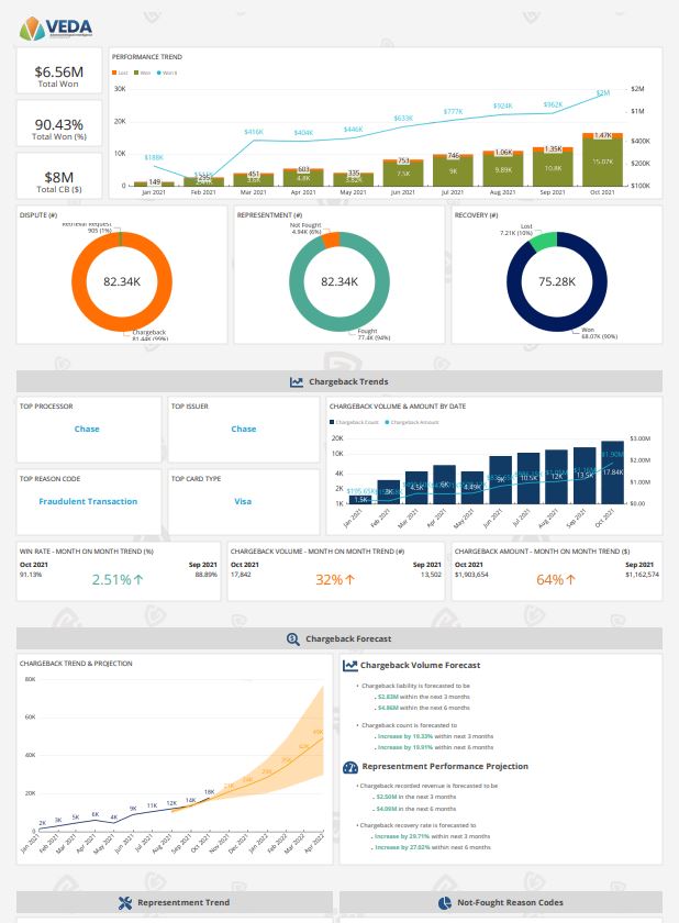
To power Veda, we were looking for a balance of flexibility and customization. We needed a BI tool that would meet our data analytics needs, and also provide us with the agility to make periodic changes to align with business requirements. The main reasons we chose QuickSight were:
- Fast setup – Speed and agility can make all the difference when it comes to gathering insights that can impact revenue lost from chargebacks.
- Comprehensive out-of-the-box functionality – Having a tool that has all the business intelligence and embedded analytics capabilities that we needed from the start was very important.
- SPICE engine – SPICE (Super-fast, Parallel, In-memory Calculation Engine) is the robust in-memory engine that QuickSight uses. As it’s engineered to rapidly perform advanced calculations and serve data, it was a big selling point for us.
QuickSight’s out-of-the-box features and functionality were the perfect fit, enabling us to get started with providing insights to our customers right away.
User-friendliness is a key differentiator
Our Gurus provide deep analytics and data-driven recommendations to help businesses identify the problems and inefficiencies that are leading to chargebacks. With this guidance, companies can permanently improve their business processes and increase customer retention. Though we have the expertise and acumen to assist with all aspects of chargeback mitigation, management, and forecasting, we needed that same level of expertise and acumen when it came to translating ideas to products in the BI space.
QuickSight has met all our needs to provide dashboards and reports, with insightful visualizations that help our customers run their businesses more efficiently. Better still, it has done so through an intuitive, user-friendly interface that enables people from all technical backgrounds to use it with very little time spent on training. Having a minimal training timeframe is a key factor when it comes to onboarding new clients.
Partners in customer obsession
One of the things that has been a delightful surprise in our experience with QuickSight is how invested the development team is in collecting our feedback and using it to help inform plans for future releases. We have agreed to be beta testers, and so we receive proactive updates on progress from the project team, providing us with informative visibility on upcoming changes. Being understanding of evolving customer and data needs, and being receptive to feedback has made this a fantastic partnership. We look forward to continuing to work with QuickSight to expand our BI capabilities, empowering our customers with the data they need to be efficient and successful.
To learn more about how QuickSight can help your business with dashboards, reports, and more, visit Amazon QuickSight.
To learn more about how Chargeback Gurus can help you solve your chargeback and fraud challenges, visit www.chargebackgurus.com or email win@chargebackgurus.com.
About the authors
 Suresh Dakshina is the Co-founder & President at Chargeback Gurus. A pioneer in data analytics and industry-specific risk management, he is a certified e-commerce fraud prevention specialist and Certified Payments Professional. He understands first-hand the challenges that business owners face, especially when it comes to chargebacks and fraud. He is a veteran speaker, and works closely with Card Networks like Visa and American Express on chargeback process optimization and compelling evidence policies. He loves spending time with his family and his Labradoodle, Joy, when not working.
 Damodharan Sampathkumar is the Chief Product Officer & GM-India at Chargeback Gurus. He is responsible for product strategy, platform development, and leading innovation for the next generation in payments technology with a specific focus on Chargebacks and Risk mitigation at Chargeback Gurus. He specializes in cloud-native, mission-critical, real-time payment systems, group-up technology platform setup, and operations. He has successfully championed multiple new-age digital payment platforms across North America, Europe, India, and the Middle East for Central Banks, Acquirer processors, and Fintech innovators. He is an avid cyclist and regular endurance rider who loves to ride during his time off to bring the right balance between work and life.
This is a guest post by Miguel Chin, Data Engineering Manager at OLX Group and David Greenshtein, Specialist Solutions Architect for Analytics, AWS.
OLX Group is one of the world’s fastest-growing networks of online marketplaces, operating in over 30 countries around the world. We help people buy and sell cars, find housing, get jobs, buy and sell household goods, and much more.
We live in a data-producing world, and as companies want to become data driven, there is the need to analyze more and more data. These analyses are often done using data warehouses. However, a common data warehouse issue with ever-growing volumes of data is storage limitations and the degrading performance that comes with it. This scenario is very familiar to us in OLX Group. Our data warehouse is built using Amazon Redshift and is used by multiple internal teams to power their products and data-driven business decisions. As such, it’s crucial to maintain a cluster with high availability and performance while also being storage cost-efficient.
In this post, we share how we modernized our Amazon Redshift data warehouse by migrating to RA3 nodes and how it enabled us to achieve our business expectations. Hopefully you can learn from our experience in case you are considering doing the same.
Status quo before migration
Here at OLX Group, Amazon Redshift has been our choice for data warehouse for over 5 years. We started with a small Amazon Redshift cluster of 7 DC2.8xlarge nodes, and as its popularity and adoption increased inside the OLX Group data community, this cluster naturally grew.
Before migrating to RA3, we were using a 16 DC2.8xlarge nodes cluster with a highly tuned workload management (WLM), and performance wasn’t an issue at all. However, we kept facing challenges with storage demand due to having more users, more data sources, and more prepared data. Almost every day we would get an alert that our disk space was close to 100%, which was about 40 TB worth of data.
Our usual method to solve storage problems used to be to simply increase the number of nodes. Overall, we reached a cluster size of 18 nodes. However, this solution wasn’t cost-efficient enough because we were adding compute capacity to the cluster even though computation power was underutilized. We saw this as a temporary solution, and we mainly did it to buy some time to explore other cost-effective alternatives, such as RA3 nodes.
Amazon Redshift RA3 nodes along with Redshift Managed Storage (RMS) provided separation of storage and compute, enabling us to scale storage and compute separately to better meet our business requirements.
Our data warehouse had the following configuration before the migration:
- 18 x DC2.8xlarge nodes
- 250 monthly active users, consistently increasing
- 10,000 queries per hour, 30 queries in parallel
- 40 TB of data, consistently increasing
- 100% disk space utilization
This cluster’s performance was generally good, ETL (extract, transform, and load) and interactive queries barely had any queue time, and 80% of them would finish in under 5 minutes.
Evaluating the performance of Amazon Redshift clusters with RA3 nodes
In this section, we discuss how we conducted a performance evaluation of RA3 nodes with an Amazon Redshift cluster.
Test environment
In order to be confident with the performance of the RA3 nodes, we decided to stress test them in a controlled environment before making the decision to migrate. To assess the nodes and find an optimal RA3 cluster configuration, we collaborated with AllCloud, the AWS premier consulting partner. The following figures illustrate the approach we took to evaluate the performance of RA3.
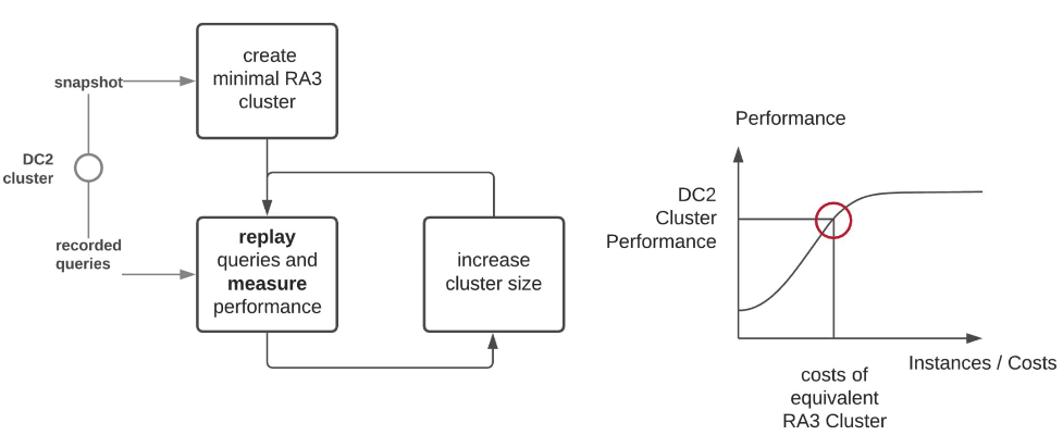
This strategy aims to replicate a realistic workload in different RA3 cluster configurations and compare them with our DC2 configuration. To do this, we required the following:
- A reference cluster snapshot – This ensures that we can replay any tests starting from the same state.
- A set of queries from the production cluster – This set can be reconstructed from the Amazon Redshift logs (
STL\_QUERYTEXT) and enriched by metadata (STL\_QUERY). It should be noted that we only took into consideration SELECT and FETCH query types (to simplify this first stage of performance tests). The following chart shows what the profile of our test set looked like.

- A replay tool to orchestrate all the query operations – AllCloud developed a Python application for us for this purpose.
For more details about approach we used, including using the Amazon Redshift Simple Replay utility, refer to Compare different node types for your workload using Amazon Redshift.
Next, we picked which cluster configurations we wanted to test, which RA3 type, and how many nodes. For the specifications of each node type, refer to Amazon Redshift pricing.
First, we decided to test the same DC2 cluster we had in production as a way to validate our test environment, followed by RA3 clusters using RA3.4xlarge nodes with various numbers of nodes. We used RA3.4xlarge because it gives us more flexibility to fine-tune how many nodes we need compared to the RA3.16xlarge instance (1 x RA3.16xlarge node is equivalent to 4 x RA3.4xlarge nodes in terms of CPU and memory). With this in mind, we tested the following cluster configurations and used the replay tool to take measurements of the performance of each cluster.
| 18 x DC2 (Reference) | 18 x RA3 (Before Classic Resize) | 18 x RA3 | 6 x RA3 | ||
| Queries | Number | 1560 | 1560 | 1560 | 1560 |
| Timeouts | – | 25 | 66 | 127 | |
| Duration/s | Mean | 1.214 | 1.037 | 1.167 | 1.921 |
| Std. | 2.268 | 2.026 | 2.525 | 3.488 | |
| Min. | 0.003 | 0.000 | 0.002 | 0.002 | |
| Q 25% | 0.005 | 0.004 | 0.004 | 0.004 | |
| Q 50% | 0.344 | 0.163 | 0.118 | 0.183 | |
| Q 75% | 1.040 | 0.746 | 1.076 | 2.566 | |
| Max. | 25.411 | 15.492 | 19.770 | 19.132 |
These results show how the DC2 cluster compares with other RA3 configurations. For 50% of the faster queries (quantile 50%) they ran faster than on DC2. Regarding the number of RA3 nodes, six nodes were clearly slower, particularly noticeable on quantile 75% of query durations.
We used the following steps to deploy different clusters:
- Use 18 x DC2.8xlarge, restored from the original snapshot (18 x DC2.8xlarge).
- Take measurements 18 x DC2.
- Use 18 x RA3.4xlarge, restored from the original snapshot (18 x DC2.8xlarge).
- Take measurements 18 x RA3 (before classic resize).
- Use 6 x RA3.4xlarge, classic resize from 18 x RA3.4xlarge.
- Take snapshot from 6 x RA3.4xlarge.
- Take measurements 6 x RA3.
- Use 6 x RA3.4xlarge, restored from 6 x RA3.4xlarge snapshot.
- Use 18 x RA3.4xlarge, elastic resize from 6 x RA3.4xlarge.
- Take measurements 18x RA3.
Although these are promising results, there were some limitations in the test environment setup. We were concerned that we weren’t stressing the clusters enough, queries were only running in sequence using a single client, and the fact that we were using only SELECT and FETCH query types moved us away from a realistic workload. Therefore, we proceeded to the second stage of our tests.
Concurrency stress test
To stress the clusters, we changed our replay tool to run multiple queries in parallel. Queries extracted from the log files were queued with the same frequency as they were originally run in the reference cluster. Up to 50 clients take queries from the queue and send them to Amazon Redshift. The timing of all queries is recorded for comparison with the reference cluster.

The cluster performance is evaluated by measuring the temporal course of the query concurrency. If a cluster is equally performant as the reference cluster, the concurrency will closely follow the concurrency of the reference cluster. Queries pushed to the query queue are immediately picked up by a client and sent to the cluster. If the cluster isn’t capable of handling the queries as fast as the reference cluster, the number of running concurrent queries will increase when compared to the reference cluster. We also decided to keep concurrency scaling disabled during this test because we wanted to focus on node types instead of cluster features.
The following table shows the concurrent queries running on a DC2 and RA3 (both 18 nodes) with two different query test sets (3:00 AM and 1:00 PM). These were selected so we could test both our day and overnight workloads. 3:00 AM is when we have a peak of automated ETL jobs running, and 1:00 PM is when we have high user activity.
The median of running concurrent queries on the RA3 cluster is much higher than the DC2 one. This led us to conclude that a cluster of 18 RA3.4xlarge might not be enough to handle this workload reliably.
| Concurrency | 18 x DC2.8xlarge | 18 x RA3.4xlarge | ||
| Starting | 3:00 AM | 1:00 PM | 3:00 AM | 1:00 PM |
| Mean | 5 | 7 | 10 | 5 |
| STD | 11 | 13 | 7 | 4 |
| 25% | 1 | 1 | 5 | 2 |
| 50% | 2 | 2 | 8 | 4 |
| 75% | 4 | 4 | 13 | 7 |
| Max | 50 | 50 | 50 | 27 |
RA3.16xlarge
Initially, we chose the RA3.4xlarge node type for more granular control in fine-tuning the number of nodes. However, we overlooked one important detail: the same instance type is used for worker and leader nodes. A leader node needs to manage all the parallel processing happening in the cluster, and a single RA3.4xlarge wasn’t enough to do so.
With this in mind, we tested two more cluster configurations: 6 x RA3.16xlarge and 8 x RA3.16xlarge, and once again measured concurrency. This time the results were much better; RA3.16xlarge was able to keep up with the reference concurrency, and the sweet spot seemed to be between 6–8 nodes.
| Concurrency | 18 x DC2.8xlarge | 18 x RA3.4xlarge | 6 x RA3.16xlarge | 8 x RA3.16xlarge | ||
| Starting | 3:00 AM | 1:00 PM | 3:00 AM | 1:00 PM | 3:00 AM | 3:00 AM |
| Mean | 5 | 7 | 10 | 5 | 3 | 1 |
| STD | 11 | 13 | 7 | 4 | 4 | 1 |
| 25% | 1 | 1 | 5 | 2 | 2 | 0 |
| 50% | 2 | 2 | 8 | 4 | 3 | 1 |
| 75% | 4 | 4 | 13 | 7 | 4 | 2 |
| Max | 50 | 50 | 50 | 27 | 38 | 9 |
Things were looking better and our target configuration was now a 7 x RA3.16xlarge cluster. We were now confident enough to proceed with the migration.
The migration
Regardless of how excited we were to proceed, we still wanted to do a calculated migration. It’s best practice to have a playbook for migrations—a step-by-step guide on what needs to be done and also a contingency plan that includes a rollback plan. For simplicity reasons, we list here only the relevant steps in case you are looking for inspiration.
Migration plan
The migration plan included the following key steps:
- Remove the DNS from the current cluster, in our case in Amazon Route 53. No users should be able to query after this.
- Check if any sessions are still running a query, and decide to wait or stop it. This strongly indicates these users are using the direct cluster URL to connect.
- To check running sessions, use
SELECT * FROM STV\_SESSIONS. - To check stopped sessions, use
SELECT PG\_TERMINATE\_BACKEND(xxxxx);.
- To check running sessions, use
- Create a snapshot of the DC2 cluster.
- Pause the DC2 cluster.
- Create an RA3 cluster from the snapshot with the following configuration:
- Node type – RA3.16xlarge
- Number of nodes – 7
- Database name – Same as the DC2
- Associated IAM roles – Same as the DC2
- VPC – Same as the DC2
- VPC security groups – Same as the DC2
- Parameter groups – Same as the DC2
- Wait for
SELECT COUNT(1) FROM STV\_UNDERREPPED\_BLOCKSto return 0. This is related to the hydration process of the cluster. - Point the DNS to the RA3 cluster.
- Users can now query the cluster again.
Contingency plan
In case the performance of hourly and daily ETL is not acceptable, the contingency plan is triggered:
- Add one more node to deal with the unexpected workload.
- Increase the limit of concurrency scaling hours.
- Reassess the parameter group.
Following this plan, we migrated from DC2 to RA3 nodes in roughly 3.5 hours, from stopping the old cluster to booting the new one and letting our processes fully synchronize. We then proceeded to monitor performance for a couple of hours. Storage capacity was looking great and everything was running smoothly, but we were curious to see how the overnight processes would perform.

The next morning, we woke up to what we dreaded: a slow cluster. We triggered our contingency plan and in the following few days we ended up implementing all three actions we had in the contingency plan.
Adding one extra node itself didn’t provide much help, however users did experience good performance during the hours concurrency scaling was on. The concurrency scaling feature allows Amazon Redshift to temporarily increase cluster capacity whenever the workload requires it. We configured it to allow a maximum of 4 hours per day—1 hour for free and 3 hours paid. We chose this particular value because price-wise it is equivalent to adding one more node (taking us to nine nodes) with the added advantage of only using and paying for it when the workload requires it.
The last action we took was related to the parameter group, in particular, the WLM. As initially stated, we had a manually fine-tuned WLM, but it proved to be inefficient for this new RA3 cluster. Therefore, we decided to try auto WLM with the following configuration.
| Manual WLM before introducing auto WLM | Queue 1 | Data Team ETL queue (daily and hourly), admin, monitoring, data quality queries |
| Queue 2 | Users queue (for both their ETL and ad hoc queries) | |
| Auto WLM | Queue 1: Priority highest | Daily Data Team ETL queue |
| Queue 2: Priority high | Admin queries | |
| Queue 3: Priority normal | User queries and hourly Data Team ETL | |
| Queue 4: Priority low | Monitoring, data quality queries |
Manual WLM requires you to manually allocate a percentage of resources and define a number of slots per queue. Although this gives you resource segregation, it also means resources are constantly allocated and can go to waste if they’re not used. Auto WLM dynamically sets these variables depending on each queue’s priority and workload. This means that a query in the highest priority queue will get all the resources allocated to it, while lower priority queues will need to wait for available resources. With this in mind, we split our ETL depending on its priority: daily ETL to highest, hourly ETL to normal (to give a fair chance for user queries to compete for resources), and monitoring and data quality to low.
After applying concurrency scaling and auto WLM, we achieved stable performance for a whole week, and considered the migration a success.
Status quo after migration
Almost a year has passed since we migrated to RA3 nodes, and we couldn’t be more satisfied. Thanks to Redshift Managed Storage (RMS), our disk space issues are a thing of the past, and performance has been generally great compared to our previous DC2 cluster. We are now at 300 monthly active users. Cluster costs did increase due to the new node type and concurrency scaling, but we now feel prepared for the future and don’t expect any cluster resizing anytime soon.
Looking back, we wanted to have a carefully planned and prepared migration, and we were able to learn more about RA3 with our test environment. However, our experience also shows that test environments aren’t always bulletproof, and some details may be overlooked. In the end, these are our main takeaways from the migration to RA3 nodes:
- Pick the right node type according to your workload. An RA3.16xlarge cluster provides more powerful leader and worker nodes.
- Use concurrency scaling to provision more resources when the workload demands it. Adding a new node is not always the most cost-efficient solution.
- Manual WLM requires a lot of adjustments; using auto WLM allows for a better and fairer distribution of cluster resources.
Conclusion
In this post, we covered how OLX Group modernized our Amazon Redshift data warehouse by migrating to RA3 nodes. We detailed how we tested before migration, the migration itself, and the outcome. We are now starting to explore the possibilities provided by the RA3 nodes. In particular, the data sharing capabilities together with Redshift Serverless open the door for exciting architecture setups that we are looking forward to.
If you are going through the same storage issues we used to face with your Amazon Redshift cluster, we highly recommend migrating to RA3 nodes. Its RMS feature decouples the scalability of compute and storage power, providing a more cost-efficient solution.
Thanks for reading this post and hopefully you found it useful. If you’re going through the same scenario and have any questions, feel free to reach out.
About the author
 Miguel Chin is a Data Engineering Manager at OLX Group, one of the world’s fastest-growing networks of trading platforms. He is responsible for managing a domain-oriented team of data engineers that helps shape the company’s data ecosystem by evangelizing cutting-edge data concepts like data mesh.
 David Greenshtein is a Specialist Solutions Architect for Analytics at AWS with a passion for ETL and automation. He works with AWS customers to design and build analytics solutions enabling business to make data-driven decisions. In his free time, he likes jogging and riding bikes with his son.
This post was co-written with Amit Shah, Principal Consultant at Atos.
Customers across industries seek meaningful insights from the data captured in their Customer Relationship Management (CRM) systems. To achieve this, they combine their CRM data with a wealth of information already available in their data warehouse, enterprise systems, or other software as a service (SaaS) applications. One widely used approach is getting the CRM data into your data warehouse and keeping it up to date through frequent data synchronization.
Integrating third-party SaaS applications is often complicated and requires significant effort and development. Developers need to understand the application APIs, write implementation and test code, and maintain the code for future API changes. Amazon AppFlow, which is a low-code/no-code AWS service, addresses this challenge.
Amazon AppFlow is a fully managed integration service that enables you to securely transfer data between SaaS applications, like Salesforce, SAP, Zendesk, Slack, and ServiceNow, and AWS services like Amazon Simple Storage Service (Amazon S3) and Amazon Redshift in just a few clicks. With Amazon AppFlow, you can run data flows at enterprise scale at the frequency you choose—on a schedule, in response to a business event, or on demand.
In this post, we focus on synchronizing your data from Salesforce to Snowflake (on AWS) without writing code. This post walks you through the steps to set up a data flow to address full and incremental data load using an example use case.
Solution overview
Our use case involves the synchronization of the Account object from Salesforce into Snowflake. In this architecture, you use Amazon AppFlow to filter and transfer the data to your Snowflake data warehouse.
You can configure Amazon AppFlow to run your data ingestion in three different ways:
- On-demand – You can manually run the flow through the AWS Management Console, API, or SDK call.
- Event-driven – Amazon AppFlow can subscribe and listen to change data capture (CDC) events from the source SaaS application.
- Scheduled – Amazon AppFlow can run schedule-triggered flows based on a pre-defined schedule rule. With scheduled flows, you can choose either full or incremental data transfer:
- With full transfer, Amazon AppFlow transfers a snapshot of all records at the time of the flow run from the source to the destination.
- With incremental transfer, Amazon AppFlow transfers only the records that have been added or changed since the last successful flow run. To determine the incremental delta of your data, AppFlow requires you to specify a source timestamp field to instruct how Amazon AppFlow identifies new or updated records.
We use the on-demand trigger for the initial load of data from Salesforce to Snowflake, because it helps you pull all the records, irrespective of their creation. To then synchronize data periodically with Snowflake, after we run the on-demand trigger, we configure a scheduled trigger with incremental transfer. With this approach, Amazon AppFlow pulls the records based on a chosen timestamp field from the Salesforce Account object periodically, based on the time interval specified in the flow.
The Account\_Staging table is created in Snowflake to act as a temporary storage that can be used to identify the data change events. Then the permanent table (Account) is updated from the staging table by running a SQL stored procedure that contains the incremental update logic. The following figure depicts the various components of the architecture and the data flow from the source to the target.

The data flow contains the following steps:
- First, the flow is run with on-demand and full transfer mode to load the full data into Snowflake.
- The Amazon AppFlow Salesforce connector pulls the data from Salesforce and stores it in the Account Data S3 bucket in CSV format.
- The Amazon AppFlow Snowflake connector loads the data into the
Account\_Stagingtable. - A scheduled task, running at regular intervals in Snowflake, triggers a stored procedure.
- The stored procedure starts an atomic transaction that loads the data into the Account table and then deletes the data from the
Account\_Stagingtable. - After the initial data is loaded, you update the flow to capture incremental updates from Salesforce. The flow trigger configuration is changed to scheduled, to capture data changes in Salesforce. This enables Snowflake to get all updates, deletes, and inserts in Salesforce at configured intervals.
- The flow uses the configured
LastModifiedDatefield to determine incremental changes. - Steps 3, 4, and 5 are run again to load the incremental updates into the Snowflake Accounts table.
Prerequisites
To get started, you need the following prerequisites:
- A Salesforce user account with sufficient privileges to install connected apps. Amazon AppFlow uses a connected app to communicate with Salesforce APIs. If you don’t have a Salesforce account, you can sign up for a developer account.
- A Snowflake account with sufficient permissions to create and configure the integration, external stage, table, stored procedures, and tasks.
- An AWS account with access to AWS Identity and Access Management (IAM), Amazon AppFlow, and Amazon S3.
Set up Snowflake configuration and Amazon S3 data
Complete the following steps to configure Snowflake and set up your data in Amazon S3:
- Create two S3 buckets in your AWS account: one for holding the data coming from Salesforce, and another for holding error records.
A best practice when creating your S3 bucket is to make sure you block public access to the bucket to ensure your data is not accessible by unauthorized users.
- Create an IAM policy named snowflake-access that allows listing the bucket contents and reading S3 objects inside the bucket.
Follow the instructions for steps 1 and 2 in Configuring a Snowflake Storage Integration to Access Amazon S3 to create an IAM policy and role. Replace the placeholders with your S3 bucket names.
- Log in to your Snowflake account and create a new warehouse called
SALESFORCEand database calledSALESTEST. - Specify the format in which data will be available in Amazon S3 for Snowflake to load (for this post, CSV):
- Amazon AppFlow uses the Snowflake COPY command to move data using an S3 bucket. To configure this integration, follow steps 3–6 in Configuring a Snowflake Storage Integration to Access Amazon S3.
These steps create a storage integration with your S3 bucket, update IAM roles with Snowflake account and user details, and creates an external stage.
This completes the setup in Snowflake. In the next section, you create the required objects in Snowflake.
Create schemas and procedures in Snowflake
In your Snowflake account, complete the following steps to create the tables, stored procedures, and tasks for implementing the use case:
- In your Snowflake account, open a worksheet and run the following DDL scripts to create the
AccountandAccount\_stagingtables:
- Create a stored procedure in Snowflake to load data from
stagingto theAccounttable:
This stored procedure determines whether the data contains new records that need to be inserted or existing records that need to be updated or deleted. After a successful run, the stored procedure clears any data from your staging table.
- Create a task in Snowflake to trigger the stored procedure. Make sure that the time interval for this task is more than the time interval configured in Amazon AppFlow for pulling the incremental changes from Salesforce. The time interval should be sufficient for data to be processed.
- Provide the required permissions to run the task and resume the task:
- As soon as task is created it will be suspended state so needs to resume it manually first time
- If the role which is assigned to us doesn’t have proper access to resume/execute task needs to grant execute task privilege to that role
This completes the Snowflake part of configuration and setup.
Create a Salesforce connection
First, let’s create a Salesforce connection that can be used by AppFlow to authenticate and pull records from your Salesforce instance. On the AWS console, make sure you are in the same Region where your Snowflake instance is running.
- On the Amazon AppFlow console, choose Connections in the navigation pane.
- From the list of connectors, select Salesforce.
- Choose Create connection.
- For Connection name, enter a name of your choice (for example,
Salesforce-blog). - Leave the rest of the fields as default and choose Continue.
- You’re redirected to a sign-in page, where you need to log in to your Salesforce instance.
- After you allow Amazon AppFlow access to your Salesforce account, your connection is successfully created.
 |  |
Create a Snowflake connection
Complete the following steps to create your Snowflake connection:
- On the Connections menu, choose Snowflake.
- Choose Create connection.
- Provide information for the Warehouse, Stage name, and Bucket details fields.
- Enter your credential details.

- For Region, choose the same Region where Snowflake is running.
- For Connection name, name your connection
Snowflake-blog. - Leave the rest of the fields as default and choose Connect.

Create a flow in Amazon AppFlow
Now you create a flow in Amazon AppFlow to load the data from Salesforce to Snowflake. Complete the following steps:
- On the Amazon AppFlow console, choose Flows in the navigation pane.
- Choose Create flow.
- On the Specify flow details page, enter a name for the flow (for example,
AccountData-SalesforceToSnowflake). - Optionally, provide a description for the flow and tags.
- Choose Next.

- On the Configure flow page, for Source name¸ choose Salesforce.
- Choose the Salesforce connection we created in the previous step (
Salesforce-blog). - For Choose Salesforce object, choose Account.
- For Destination name, choose Snowflake.
- Choose the newly created Snowflake connection.
- For Choose Snowflake object, choose the staging table you created earlier (
SALESTEST.PUBLIC. ACCOUNT\_STAGING).

- In the Error handling section, provide your error S3 bucket.
- For Choose how to trigger the flow¸ select Run on demand.
- Choose Next.

- Select Manually map fields to map the fields between your source and destination.
- Choose the fields
Account Number,Account Name,Account Type,Annual Revenue,Active,Deleted, andLast Modified Date.

- Map each source field to its corresponding destination field.
- Under Additional settings, leave the Import deleted records unchecked (default setting).

- In the Validations section, add validations for the data you’re pulling from Salesforce.
Because the schema for the Account\_Staging table in Snowflake database has a NOT NULL constraint for the fields Account\_Number and Active, records containing a null value for these fields should be ignored.
- Choose Add Validation to configure validations for these fields.
- Choose Next.

- Leave everything else as default, proceed to the final page, and choose Create Flow.
- After the flow is created, choose Run flow.

When the flow run completes successfully, it will bring all records into your Snowflake staging table.

Verify data in Snowflake
The data will be loaded into the Account\_staging table. To verify that data is loaded in Snowflake, complete the following steps:
- Validate the number of records by querying the
ACCOUNT\_STAGINGtable in Snowflake. - Wait for your Snowflake task to run based on the configured schedule.
- Verify that all the data is transferred to the
ACCOUNTtable and theACCOUNT\_STAGINGtable is truncated.
Configure an incremental data load from Salesforce
Now let’s configure an incremental data load from Salesforce:
- On the Amazon AppFlow console, select your flow, and choose Edit.
- Go to the Edit configuration step and change to Run flow on schedule.
- Set the flow to run every 5 minutes, and provide a start date of Today, with a start time in the future.
- Choose Incremental transfer and choose the
LastModifiedDatefield. - Choose Next.
- In the Additional settings section, select Import deleted records.
This ensures that deleted records from the source are also ingested.
- Choose Save and then choose Activate flow.
Now your flow is configured to capture all incremental changes.
Test the solution
Log in to your Salesforce account, and edit any record in the Account object.
Within 5 minutes or less, a scheduled flow will pick up your change and write the changed record into your Snowflake staging table and trigger the synchronization process.

You can see the details of the run, including number of records transferred, on the Run History tab of your flow.

Clean up
Clean up the resources in your AWS account by completing the following steps:
- On the Amazon AppFlow console, choose Flows in the navigation pane.
- From the list of flows, select the flow
AccountData-SalesforceToSnowflakeanddelete it. - Enter delete to delete the flow.
- Choose Connections in the navigation pane.
- Choose Salesforce from the list of connectors, select
Salesforce-blog, and delete it. - Enter delete to delete the connector.
- On the Connections page, choose Snowflake from the list of connectors, select
Snowflake-blog, and delete it. - Enter delete to delete the connector.
- On the IAM console, choose Roles in the navigation page, then select the role you created for Snowflake and delete it.
- Choose Policies in the navigation pane, select the policy you created for Snowflake, and delete it.
- On the Amazon S3 console, search for the data bucket you created, choose Empty to delete the objects, then delete the bucket.
- Search for the error bucket you created, choose Empty to delete the objects, then delete the bucket.
- Clean up resources in your Snowflake account:
- Delete the task
TASK\_ACCOUNT\_LOAD:
- Delete the stored procedure
sp\_account\_load:
- Delete the tables
ACCOUNT\_STAGINGandACCOUNT:
Conclusion
In this post, we walked you through how to integrate and synchronize your data from Salesforce to Snowflake using Amazon AppFlow. This demonstrates how you can set up your ETL jobs without having to learn new programming languages by using Amazon AppFlow and your familiar SQL language. This is a proof of concept, but you can try to handle edge cases like failure of Snowflake tasks or understand how incremental transfer works by making multiple changes to a Salesforce record within the scheduled time interval.
For more information on Amazon AppFlow, visit Amazon AppFlow.
About the authors
 Ramesh Ranganathan is a Senior Partner Solution Architect at AWS. He works with AWS customers and partners to provide guidance on enterprise cloud adoption, application modernization and cloud native development. He is passionate about technology and enjoys experimenting with AWS Serverless services.
 Kamen Sharlandjiev is an Analytics Specialist Solutions Architect and Amazon AppFlow expert. He’s on a mission to make life easier for customers who are facing complex data integration challenges. His secret weapon? Fully managed, low-code AWS services that can get the job done with minimal effort and no coding.
 Amit Shah is a cloud based modern data architecture expert and currently leading AWS Data Analytics practice in Atos. Based in Pune in India, he has 20+ years of experience in data strategy, architecture, design and development. He is on a mission to help organization become data-driven.
Amazon Redshift is a fully managed, petabyte-scale data warehouse service in the cloud. Amazon Redshift enables you to run complex SQL analytics at scale and performance on terabytes to petabytes of structured and unstructured data, and make the insights widely available through popular business intelligence (BI) and analytics tools.
It’s common to ingest multiple data sources into Amazon Redshift to perform analytics. Often, each data source will have its own processes of creating and maintaining data, which can lead to data quality challenges within and across sources.
One challenge you may face when performing analytics is the presence of imperfect duplicate records within the source data. Answering questions as simple as “How many unique customers do we have?” can be very challenging when the data you have available is like the following table.
| Name | Address | Date of Birth |
| Cody Johnson | 8 Jeffery Brace, St. Lisatown | 1/3/1956 |
| Cody Jonson | 8 Jeffery Brace, St. Lisatown | 1/3/1956 |
Although humans can identify that Cody Johnson and Cody Jonson are most likely the same person, it can be difficult to distinguish this using analytics tools. This identification of duplicate records also becomes nearly impossible when working on large datasets across multiple sources.
This post presents one possible approach to addressing this challenge in an Amazon Redshift data warehouse. We import an open-source fuzzy matching Python library to Amazon Redshift, create a simple fuzzy matching user-defined function (UDF), and then create a procedure that weights multiple columns in a table to find matches based on user input. This approach allows you to use the created procedure to approximately identify your unique customers, improving the accuracy of your analytics.
This approach doesn’t solve for data quality issues in source systems, and doesn’t remove the need to have a wholistic data quality strategy. For addressing data quality challenges in Amazon Simple Storage Service (Amazon S3) data lakes and data pipelines, AWS has announced AWS Glue Data Quality (preview). You can also use AWS Glue DataBrew, a visual data preparation tool that makes it easy for data analysts and data scientists to clean and normalize data to prepare it for analytics.
Prerequisites
To complete the steps in this post, you need the following:
- An AWS account.
- An Amazon Redshift cluster or Amazon Redshift Serverless endpoint.
- An S3 bucket.
- The open-source Python package TheFuzz—from this link, you need all files in the folder
thefuzzzipped and uploaded to the S3 bucket. - An AWS Identity and Access Management (IAM) role that provides read access to the created S3 bucket. This role will need to be set as the default role on the Amazon Redshift cluster or endpoint for the following steps to work.
The following AWS CloudFormation stack will deploy a new Redshift Serverless endpoint and an S3 bucket for use in this post.
All SQL commands shown in this post are available in the following notebook, which can be imported into the Amazon Redshift Query Editor V2.
Overview of the dataset being used
The dataset we use is mimicking a source that holds customer information. This source has a manual process of inserting and updating customer data, and this has led to multiple instances of non-unique customers being represented with duplicate records.
The following examples show some of the data quality issues in the dataset being used.
In this first example, all three customers are the same person but have slight differences in the spelling of their names.
| id | name | age | address\_line1 | city | postcode | state |
| 1 | Cody Johnson | 80 | 8 Jeffrey Brace | St. Lisatown | 2636 | South Australia |
| 101 | Cody Jonson | 80 | 8 Jeffrey Brace | St. Lisatown | 2636 | South Australia |
| 121 | Kody Johnson | 80 | 8 Jeffrey Brace | St. Lisatown | 2636 | South Australia |
In this next example, the two customers are the same person with slightly different addresses.
| id | name | age | address\_line1 | city | postcode | state |
| 7 | Angela Watson | 59 | 3/752 Bernard Follow | Janiceberg | 2995 | Australian Capital Territory |
| 107 | Angela Watson | 59 | 752 Bernard Follow | Janiceberg | 2995 | Australian Capital Territory |
In this example, the two customers are different people with the same address. This simulates multiple different customers living at the same address who should still be recognized as different people.
| id | name | age | address\_line1 | city | postcode | state |
| 6 | Michael Hunt | 69 | 8 Santana Rest | St. Jessicamouth | 2964 | Queensland |
| 106 | Sarah Hunt | 69 | 8 Santana Rest | St. Jessicamouth | 2964 | Queensland |
Load the dataset
First, create a new table in your Redshift Serverless endpoint and copy the test data into it by doing the following:
- Open the Query Editor V2 and log in using the admin user name and details defined when the endpoint was created.
- Run the following CREATE TABLE statement:

- Run the following COPY command to copy data into the newly created table:
- Confirm the COPY succeeded and there are 110 records in the table by running the following query:
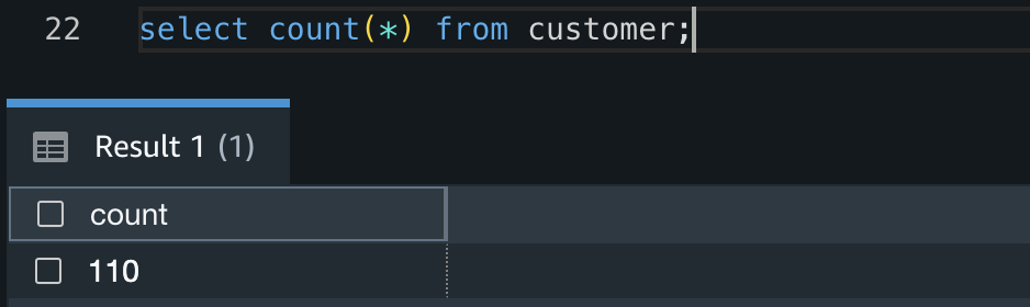
Fuzzy matching
Fuzzy string matching, more formally known as approximate string matching, is the technique of finding strings that match a pattern approximately rather than exactly. Commonly (and in this solution), the Levenshtein distance is used to measure the distance between two strings, and therefore their similarity. The smaller the Levenshtein distance between two strings, the more similar they are.
In this solution, we exploit this property of the Levenshtein distance to estimate if two customers are the same person based on multiple attributes of the customer, and it can be expanded to suit many different use cases.
This solution uses TheFuzz, an open-source Python library that implements the Levenshtein distance in a few different ways. We use the partial\_ratio function to compare two strings and provide a result between 1–100. If one of the strings matches perfectly with a portion of the other, the partial\_ratio function will return 100.
Weighted fuzzy matching
By adding a scaling factor to each of our column fuzzy matches, we can create a weighted fuzzy match for a record. This is especially useful in two scenarios:
- We have more confidence in some columns of our data than others, and therefore want to prioritize their similarity results.
- One column is much longer than the others. A single character difference in a long string will have much less impact on the Levenshtein distance than a single character difference in a short string. Therefore, we want to prioritize long string matches over short string matches.
The solution in this post applies weighted fuzzy matching based on user input defined in another table.
Create a table for weight information
This reference table holds two columns; the table name and the column mapping with weights. The column mapping is held in a SUPER datatype, which allows JSON semistructured data to be inserted and queried directly in Amazon Redshift. For examples on how to query semistructured data in Amazon Redshift, refer to Querying semistructured data.
In this example, we apply the largest weight to the column address\_line1 (0.5) and the smallest weight to the city and postcode columns (0.1).
Using the Query Editor V2, create a new table in your Redshift Serverless endpoint and insert a record by doing the following:
- Run the following CREATE TABLE statement:
- Run the following INSERT statement:
- Confirm the mapping data has inserted into the table correctly by running the following query:

- To check all weights for the
customertable add up to 1 (100%), run the following query: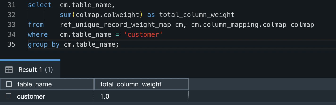
User-defined functions
With Amazon Redshift, you can create custom scalar user-defined functions (UDFs) using a Python program. A Python UDF incorporates a Python program that runs when the function is called and returns a single value. In addition to using the standard Python functionality, you can import your own custom Python modules, such as the module described earlier (TheFuzz).
In this solution, we create a Python UDF to take two input values and compare their similarity.
Import external Python libraries to Amazon Redshift
Run the following code snippet to import the TheFuzz module into Amazon Redshift as a new library. This makes the library available within Python UDFs in the Redshift Serverless endpoint. Make sure to provide the name of the S3 bucket you created earlier.
Create a Python user-defined function
Run the following code snippet to create a new Python UDF called unique\_record. This UDF will do the following:
- Take two input values that can be of any data type as long as they are the same data type (such as two integers or two varchars).
- Import the newly created
thefuzzPython library. - Return an integer value comparing the partial ratio between the two input values.
You can test the function by running the following code snippet:
The result shows that these two strings are have a similarity value of 91%.
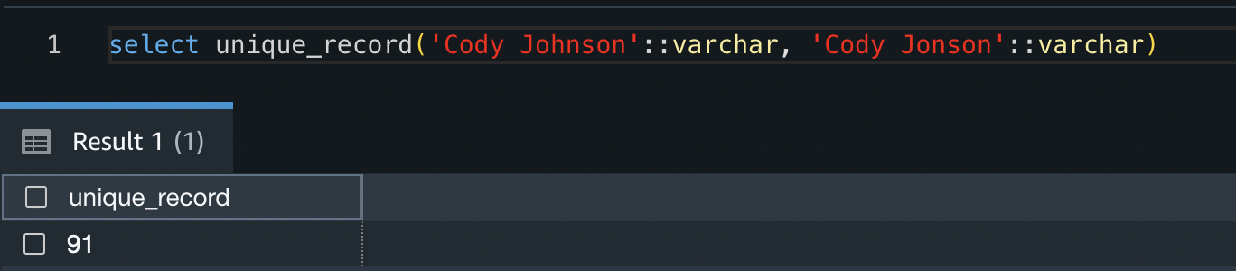
Now that the Python UDF has been created, you can test the response of different input values.
Alternatively, you can follow the amazon-redshift-udfs GitHub repo to install the f\_fuzzy\_string\_match Python UDF.
Stored procedures
Stored procedures are commonly used to encapsulate logic for data transformation, data validation, and business-specific logic. By combining multiple SQL steps into a stored procedure, you can reduce round trips between your applications and the database.
In this solution, we create a stored procedure that applies weighting to multiple columns. Because this logic is common and repeatable regardless of the source table or data, it allows us to create the stored procedure once and use it for multiple purposes.
Create a stored procedure
Run the following code snippet to create a new Amazon Redshift stored procedure called find\_unique\_id. This procedure will do the following:
- Take one input value. This value is the table you would like to create a golden record for (in our case, the
customertable). - Declare a set of variables to be used throughout the procedure.
- Check to see if weight data is in the staging table created in previous steps.
- Build a query string for comparing each column and applying weights using the weight data inserted in previous steps.
- For each record in the input table that doesn’t have a unique record ID (URID) yet, it will do the following:
- Create a temporary table to stage results. This temporary table will have all potential URIDs from the input table.
- Allocate a similarity value to each URID. This value specifies how similar this URID is to the record in question, weighted with the inputs defined.
- Choose the closest matched URID, but only if there is a >90% match.
- If there is no URID match, create a new URID.
- Update the source table with the new URID and move to the next record.
This procedure will only ever look for new URIDs for records that don’t already have one allocated. Therefore, rerunning the URID procedure multiple times will have no impact on the results.
Now that the stored procedure has been created, create the unique record IDs for the customer table by running the following in the Query Editor V2. This will update the urid column of the customer table.
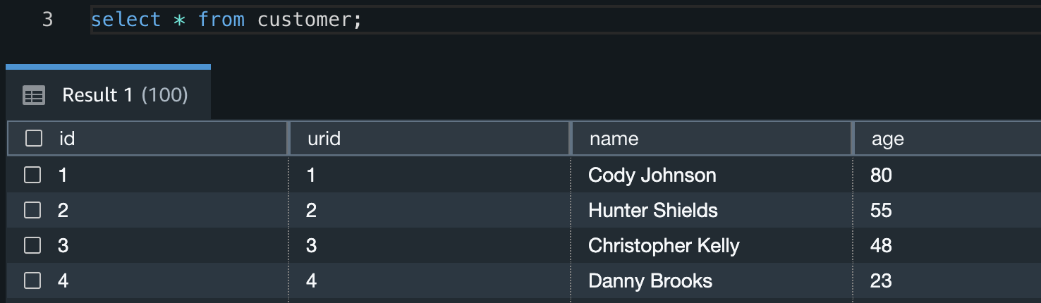
When the procedure has completed its run, you can identify what duplicate customers were given unique IDs by running the following query:

From this you can see that IDs 1, 101, and 121 have all been given the same URID, as have IDs 7 and 107.
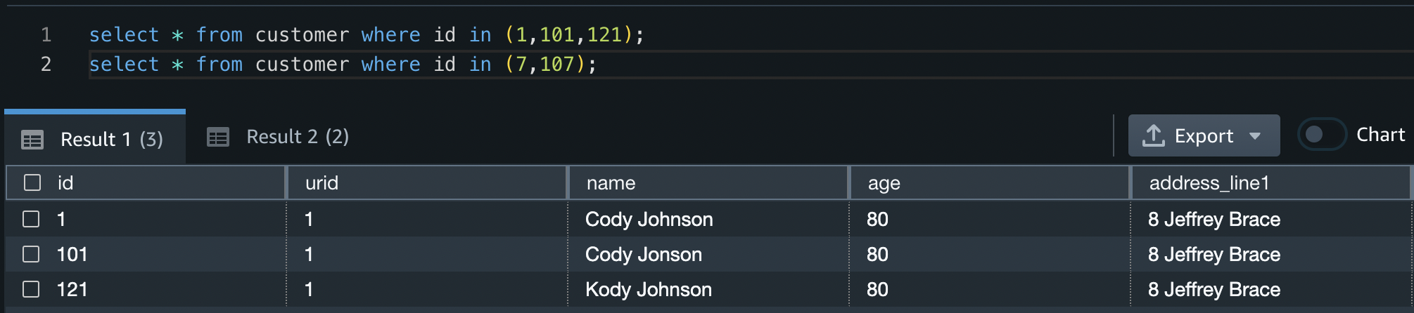
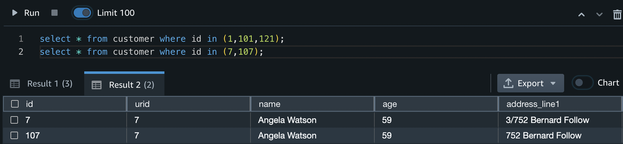
The procedure has also correctly identified that IDs 6 and 106 are different customers, and they therefore don’t have the same URID.

Clean up
To avoid incurring future reoccurring charges, delete all files in the S3 bucket you created. After you delete the files, go to the AWS CloudFormation console and delete the stack deployed in this post. This will delete all created resources.
Conclusion
In this post, we showed one approach to identifying imperfect duplicate records by applying a fuzzy matching algorithm in Amazon Redshift. This solution allows you to identify data quality issues and apply more accurate analytics to your dataset residing in Amazon Redshift.
We showed how you can use open-source Python libraries to create Python UDFs, and how to create a generic stored procedure to identify imperfect matches. This solution is extendable to provide any functionality required, including adding as a regular process in your ELT (extract, load, and transform) workloads.
Test the created procedure on your datasets to investigate the presence of any imperfect duplicates, and use the knowledge learned throughout this post to create stored procedures and UDFs to implement further functionality.
If you’re new to Amazon Redshift, refer to Getting started with Amazon Redshift for more information and tutorials on Amazon Redshift. You can also refer to the video Get started with Amazon Redshift Serverless for information on starting with Redshift Serverless.
About the Author

Sean Beath is an Analytics Solutions Architect at Amazon Web Services. He has experience in the full delivery lifecycle of data platform modernisation using AWS services and works with customers to help drive analytics value on AWS.
This is a guest post by Siva Manickam and Prahalathan M from Vyaire Medical Inc.
Vyaire Medical Inc. is a global company, headquartered in suburban Chicago, focused exclusively on supporting breathing through every stage of life. Established from legacy brands with a 65-year history of pioneering breathing technology, the company’s portfolio of integrated solutions is designed to enable, enhance, and extend lives.

At Vyaire, our team of 4,000 pledges to advance innovation and evolve what’s possible to ensure every breath is taken to its fullest. Vyaire’s products are available in more than 100 countries and are recognized, trusted, and preferred by specialists throughout the respiratory community worldwide. Vyaire has 65-year history of clinical experience and leadership with over 27,000 unique products and 370,000 customers worldwide.
Vyaire Medical’s applications landscape has multiple ERPs, such as SAP ECC, JD Edwards, Microsoft Dynamics AX, SAP Business One, Pointman, and Made2Manage. Vyaire uses Salesforce as our CRM platform and the ServiceMax CRM add-on for managing field service capabilities. Vyaire developed a custom data integration platform, iDataHub, powered by AWS services such as AWS Glue, AWS Lambda, and Amazon API Gateway.
In this post, we share how we extracted data from SAP ERP using AWS Glue and the SAP SDK.
Business and technical challenges
Vyaire is working on deploying the field service management solution ServiceMax (SMAX, a natively built on SFDC ecosystem), offering features and services that help Vyaire’s Field Services team improve asset uptime with optimized in-person and remote service, boost technician productivity with the latest mobile tools, and deliver metrics for confident decision-making.
A major challenge with ServiceMax implementation is building a data pipeline between ERP and the ServiceMax application, precisely integrating pricing, orders, and primary data (product, customer) from SAP ERP to ServiceMax using Vyaire’s custom-built integration platform iDataHub.
Solution overview
Vyaire’s iDataHub powered by AWS Glue has been effectively used for data movement between SAP ERP and ServiceMax.
AWS Glue a serverless data integration service that makes it easy to discover, prepare, and combine data for analytics, machine learning (ML), and application development. It’s used in Vyaire’s Enterprise iDatahub Platform for facilitating data movement across different systems, however the focus for this post is to discuss the integration between SAP ERP and Salesforce SMAX.
The following diagram illustrates the integration architecture between Vyaire’s Salesforce ServiceMax and SAP ERP system.

In the following sections, we walk through setting up a connection to SAP ERP using AWS Glue and the SAP SDK through remote function calls. The high-level steps are as follows:
- Clone the PyRFC module from GitHub.
- Set up the SAP SDK on an Amazon Elastic Compute Cloud (Amazon EC2) machine.
- Create the PyRFC wheel file.
- Merge SAP SDK files into the PyRFC wheel file.
- Test the connection with SAP using the wheel file.
Prerequisites
For this walkthrough, you should have the following:
- An AWS account.
- The Linux version of NW RFC SDK from a SAP licensed source. For more information, refer to Download and Installation of NW RFC SDK.
- The AWS Command Line Interface (AWS CLI) configured. For instructions, refer to Configuration basics.
Clone the PyRFC module from GitHub
For instructions for creating and connecting to an Amazon Linux 2 AMI EC2 instance, refer to Tutorial: Get started with Amazon EC2 Linux instances.
The reason we choose Amazon Linux EC2 is to compile the SDK and PyRFC in a Linux environment, which is compatible with AWS Glue.
At the time of writing this post, AWS Glue’s latest supported Python version is 3.7. Ensure that the Amazon EC2 Linux Python version and AWS Glue Python version are the same. In the following instructions, we install Python 3.7 in Amazon EC2; we can follow the same instructions to install future versions of Python.
- In the bash terminal of the EC2 instance, run the following command:
- Log in to the Linux terminal, install git, and clone the PyRFC module using the following commands:

Set up the SAP SDK on an Amazon EC2 machine
To set up the SAP SDK, complete the following steps:
- Download the
nwrfcsdk.zipfile from a licensed SAP source to your local machine. - In a new terminal, run the following command on the EC2 instance to copy the
nwrfcsdk.zipfile from your local machine to theaws\_to\_sapfolder.
 Unzip the
 nwrfcsdk.zipfile in the current EC2 working directory and verify the contents:
unzip nwrfcsdk.zip

- Configure the SAP SDK environment variable
SAPNWRFC\_HOMEand verify the contents:

Create the PyRFC wheel file
Complete the following steps to create your wheel file:
- On the EC2 instance, install Python modules cython and wheel for generating wheel files using the following command:
- Navigate to the PyRFC directory you created and run the following command to generate the wheel file:

Verify that the pyrfc-2.5.0-cp37-cp37m-linux\_x86\_64.whl wheel file is created as in the following screenshot in the PyRFC/dist folder. Note that you may see a different wheel file name based on the latest PyRFC version on GitHub.


Merge SAP SDK files into the PyRFC wheel file
To merge the SAP SDK files, complete the following steps:
- Unzip the wheel file you created:

- Copy the contents of lib (the SAP SDK files) to the pyrfc folder:

Now you can update the rpath of the SAP SDK binaries using the PatchELF utility, a simple utility for modifying existing ELF executables and libraries.
- Install the supporting dependencies (gcc, gcc-c++, python3-devel) for the Linux utility function PatchELF:
Download and install PatchELF:
- Run patchelf:
- Update the wheel file with the modified pyrfc and dist-info folders:

- Copy the wheel file
pyrfc-2.5.0-cp37-cp37m-linux\_x86\_64.whlfrom Amazon EC2 to Amazon Simple Storage Service (Amazon S3):


Test the connection with SAP using the wheel file
The following is a working sample code to test the connectivity between the SAP system and AWS Glue using the wheel file.
- On the AWS Glue Studio console, choose Jobs in the navigation pane.
- Select Spark script editor and choose Create.

- Overwrite the boilerplate code with the following code on the Script tab:
- On the Job details tab, fill in mandatory fields.
- In the Advanced properties section, provide the S3 URI of the wheel file in the Job parameters section as a key value pair:
- Key –
--additional-python-modules - Value –
s3://<bucket\_name>/ec2-dump/pyrfc-2.5.0-cp37-cp37m-linux\_x86\_64.whl(provide your S3 bucket name)
- Key –

- Save the job and choose Run.
Verify SAP connectivity
Complete the following steps to verify SAP connectivity:
- When the job run is complete, navigate to the Runs tab on the Jobs page and choose Output logs in the logs section.
- Choose the job\_id and open the detailed logs.
- Observe the message
SAP Connection successful – connection object: <connection object>, which confirms a successful connection with the SAP system. - Observe the message Successfully extracted data from SAP using custom RFC – Printing the top 5 rows, which confirms successful access of data from the SAP system.

Conclusion
AWS Glue facilitated the data extraction, transformation, and loading process from different ERPs into Salesforce SMAX to improve Vyaire’s products and its related information visibility to service technicians and tech support users.
In this post, you learned how you can use AWS Glue to connect to SAP ERP utilizing SAP SDK remote functions. To learn more about AWS Glue, check out AWS Glue Documentation.
About the Authors
 Siva Manickam is the Director of Enterprise Architecture, Integrations, Digital Research & Development at Vyaire Medical Inc. In this role, Mr. Manickam is responsible for the company’s corporate functions (Enterprise Architecture, Enterprise Integrations, Data Engineering) and produce function (Digital Innovation Research and Development).
 Prahalathan M is the Data Integration Architect at Vyaire Medical Inc. In this role, he is responsible for end-to-end enterprise solutions design, architecture, and modernization of integrations and data platforms using AWS cloud-native services.
Deenbandhu Prasad is a Senior Analytics Specialist at AWS, specializing in big data services. He is passionate about helping customers build modern data architecture on the AWS Cloud. He has helped customers of all sizes implement data management, data warehouse, and data lake solutions.
In the data analytics space, organizations often deal with many tables in different databases and file formats to hold data for different business functions. Business needs often drive table structure, such as schema evolution (the addition of new columns, removal of existing columns, update of column names, and so on) for some of these tables in one business function that requires other business functions to replicate the same. This post focuses on such schema changes in file-based tables and shows how to automatically replicate the schema evolution of structured data from table formats in databases to the tables stored as files in cost-effective way.
AWS Glue is a serverless data integration service that makes it easy to discover, prepare, and combine data for analytics, machine learning (ML), and application development. In this post, we show how to use Apache Hudi, a self-managing database layer on file-based data lakes, in AWS Glue to automatically represent data in relational form and manage their schema evolution at scale using Amazon Simple Storage Service (Amazon S3), AWS Database Migration Service (AWS DMS), AWS Lambda, AWS Glue, Amazon DynamoDB, Amazon Aurora, and Amazon Athena to automatically identify schema evolution and apply it to manage data load at petabyte scale.
Apache Hudi supports ACID transactions and CRUD operations on a data lake. This lays the foundation of a data lake architecture by enabling transaction support and schema evolution and management, decoupling storage from compute, and ensuring support for accessibility through business intelligence (BI) tools. In this post, we implement an architecture to build a transactional data lake built on the aforementioned Hudi features.
Solution overview
This post assumes a scenario where multiple tables are present in a source database, and we want to replicate any schema changes in any of those tables in Apache Hudi tables in the data lake. It uses the native support for Apache Hudi on AWS Glue for Apache Spark.
In this post, the schema evolution of source tables in the Aurora database is captured via the AWS DMS incremental load or change data capture (CDC) mechanism, and the same schema evolution is replicated in Apache Hudi tables stored in Amazon S3. Apache Hudi tables are discovered by the AWS Glue Data Catalog and queried by Athena. An AWS Glue job, supported by an orchestration pipeline using Lambda and a DynamoDB table, takes care of the automated replication of schema evolution in the Apache Hudi tables.
We use Aurora as a sample data source, but any data source that supports Create, Read, Update, and Delete (CRUD) operations can replace Aurora in your use case.
The following diagram illustrates our solution architecture.

The flow of the solution is as follows:
- Aurora, as a sample data source, contains a RDBMS table with multiple rows, and AWS DMS does the full load of that data to an S3 bucket (which we call the raw bucket). We expect that you may have multiple source tables, but for demonstration purposes, we only use one source table in this post.
- We trigger a Lambda function with the source table name as an event so that the corresponding parameters of the source table are read from DynamoDB. To schedule this operation for specific time intervals, we schedule Amazon EventBridge to trigger the Lambda with the table name as a parameter.
- There are many tables in the source database, and we want to run one AWS Glue job for each source table for simplicity in operations. Because we use each AWS Glue job to update each Apache Hudi table, this post uses a DynamoDB table to hold the configuration parameters used by each AWS Glue job for each Apache Hudi table. The DynamoDB table contains each Apache Hudi table name, corresponding AWS Glue job name, AWS Glue job status, load status (full or delta), partition key, record key, and schema to pass to the corresponding table’s AWS Glue Job. The values in the DynamoDB table are static values.
- To trigger each AWS Glue job (10 G.1X DPUs) in parallel to run an Apache Hudi specific code to insert data in the corresponding Hudi tables, Lambda passes each Apache Hudi table specific parameters read from DynamoDB to each AWS Glue job. The source data comes from tables in the Aurora source database via AWS DMS with full load and incremental load or CDC.
Create resources with AWS CloudFormation
We provide an AWS CloudFormation template to create the following resources:
- Lambda and DynamoDB as the data load management orchestrators
- S3 buckets for the raw, refined zone, and assets for holding code for schema evolution
- An AWS Glue job to update the Hudi tables and perform schema evolution, both forward- and backward-compatible
The Aurora table and AWS DMS replication instance is not provisioned via this stack. For instructions to set up Aurora, refer to Creating an Amazon Aurora DB cluster.
Launch the following stack and provide your stack name.
eu-west-1 | |
Schema evolution
To access your Aurora database, refer to How do I connect to my Amazon RDS for MySQL instance by using MySQL Workbench. Then complete the following steps:
- Create a table named object following the queries in the Aurora database and change its schema so that we can see the schema evolution is reflected at the data lake level:
After you create the stacks, some manual steps are needed to prepare the solution end to end.
- Create an AWS DMS instance, AWS DMS endpoints, and AWS DMS task with the following configurations:
- Add dataFormat as Parquet in the target endpoint.
- Point the target endpoint of AWS DMS to the raw bucket, which is formatted as
raw-bucket-<account\_number>-<region\_name>, and the folder name should be POC.
- Start the AWS DMS task.
- Create a test event in the
HudiLambdaLambda function with the content of the event JSON asPOC.dband save it. - Run the Lambda function.
In this post, the schema evolution is reflected through Hudi Hive sync in AWS Glue. You don’t alter queries separately in the data lake.
Now we complete the following steps to change the schema at the source. Trigger the Lambda function after each step to generate a file in the POC/db/object folder within the raw bucket. AWS DMS almost instantly picks up the schema changes and reports to the raw bucket.
- Add a column called
test\_columnto the source tableobjectin your Aurora database:
- Rename the column
new\_field\_1tonew\_field\_2in the source table object:
The column new\_field\_1 is expected to stay in the Hudi table but without any new values being populated to it anymore.
- Delete the column
new\_field\_2from the source table object:
Similar to the previous operation, the column new\_field\_2 is expected to stay in the Hudi table but without any new values being populated to it anymore.
If you already have AWS Lake Formation data permissions set up in your account, you may encounter permission issues. In that case, grant full permission (Super) to the default database (before triggering the Lambda function) and all tables in the POC.db database (after the load is complete).
Review the results
When the aforementioned run happens after schema changes, the following results are generated in the refined bucket. We can view the Apache Hudi tables with its contents in Athena. To set up Athena, refer to Getting started.
The table and the database are available in the AWS Glue Data Catalog and ready for browsing the schema.
Before the schema change, the Athena results look like the following screenshot.

After you add the column test\_column and insert a value in the test\_column field in the object table in the Aurora database, the new column (test\_column) is reflected in its corresponding Apache Hudi table in the data lake.
The following screenshot shows the results in Athena.

After you rename the column new\_field\_1 to new\_field\_2 and insert a value in the new\_field\_2 field in the object table, the renamed column (new\_field\_2) is reflected in its corresponding Apache Hudi table in the data lake, and new\_field\_1 remains in the schema, having no new value populated to the column.
The following screenshot shows the results in Athena.

After you delete the column new\_field\_2 in the object table and insert or update any values under any columns in the object table, the deleted column (new\_field\_2) remains in the corresponding Apache Hudi table schema, having no new value populated to the column.
The following screenshot shows the results in Athena.

Clean up
When you’re done with this solution, delete the sample data in the raw and refined S3 buckets and delete the buckets.
Also, delete the CloudFormation stack to remove all the service resources used in this solution.
Conclusion
This post showed how to implement schema evolution with an open-source solution using Apache Hudi in an AWS environment with an orchestration pipeline.
You can explore the different configurations of AWS Glue to change the AWS Glue job structures and implement it for your data analytics and other use cases.
About the Authors
 Subhro Bose is a Senior Data Architect in Emergent Technologies and Intelligence Platform in Amazon. He loves solving science problems with emergent technologies such as AI/ML, big data, quantum, and more to help businesses across different industry verticals succeed within their innovation journey. In his spare time, he enjoys playing table tennis, learn theories of environmental economics and explore the best muffins across the city.
 Ketan Karalkar is a Big Data Solutions Consultant at AWS. He has nearly 2 decades of experience helping customers design and build data analytics, and database solutions. He believes in using technology as an enabler to solve real life business problems.
 Eva Fang is a Data Scientist within Professional Services in AWS. She is passionate about using the technology to provide value to customers and achieve business outcomes. She is based in London, in her spare time, she likes to watch movies and musicals.
In the post Introducing the AWS ProServe Hadoop Migration Delivery Kit TCO tool, we introduced the AWS ProServe Hadoop Migration Delivery Kit (HMDK) TCO tool and the benefits of migrating on-premises Hadoop workloads to Amazon EMR. In this post, we dive deep into the tool, walking through all steps from log ingestion, transformation, visualization, and architecture design to calculate TCO.
Solution overview
Let’s briefly visit the HMDK TCO tool’s key features. The tool provides a YARN log collector to connect Hadoop Resource Manager to collect YARN logs. A Python-based Hadoop workload analyzer, called the YARN log analyzer, scrutinizes Hadoop applications. Amazon QuickSight dashboards showcase the results from the analyzer. The same results also accelerate the design of future EMR instances. Additionally, a TCO calculator generates the TCO estimation of an optimized EMR cluster for facilitating the migration.
Now let’s look at how the tool works. The following diagram illustrates the end-to-end workflow.

In the next sections, we walk through the five main steps of the tool:
- Collect YARN job history logs.
- Transform the job history logs from JSON to CSV.
- Analyze the job history logs.
- Design an EMR cluster for migration.
- Calculate the TCO.
Prerequisites
Before getting started, make sure to complete the following prerequisites:
- Clone the hadoop-migration-assessment-tco repository.
- Install Python 3 on your local machine.
- Have an AWS account with permission on AWS Lambda, QuickSight (Enterprise edition), and AWS CloudFormation.
Collect YARN job history logs
First, you run a YARN log collector, start-collector.sh, on your local machine. This step collects Hadoop YARN logs and places the logs on your local machine. The script connects your local machine with the Hadoop primary node and communicates with Resource Manager. Then it retrieves the job history information (YARN logs from application managers) by calling the YARN ResourceManager application API.
Prior to running the YARN log collector, you need to configure and establish the connection (HTTP: 8088 or HTTPS: 8090; the latter is recommended) to verify the accessibility of YARN ResourceManager and enabled YARN Timeline Server (Timeline Server v1 or later are supported). You may need to define the YARN logs’ collection interval and retention policy. To ensure that you collect consecutive YARN logs, you can use a cron job to schedule the log collector in a proper time interval. For example, for a Hadoop cluster with 2,000 daily applications and the setting yarn.resourcemanager.max-completed-applications set to 1,000, theoretically, you have to run the log collector at least twice to get all the YARN logs. In addition, we recommend collecting at least 7 days of YARN logs for analyzing holistic workloads.
For more details on how to configure and schedule the log collector, refer to the yarn-log-collector GitHub repo.
Transform the YARN job history logs from JSON to CSV
After obtaining YARN logs, you run a YARN log organizer, yarn-log-organizer.py, which is a parser to transform JSON-based logs to CSV files. These output CSV files are the inputs for the YARN log analyzer. The parser also has other capabilities, including sorting events by time, removing dedicates, and merging multiple logs.
For more information on how to use the YARN log organizer, refer to the yarn-log-organizer GitHub repo.
Analyze the YARN job history logs
Next, you launch the YARN log analyzer to analyze the YARN logs in CSV format.
With QuickSight, you can visualize YARN log data and conduct analysis against the datasets generated by pre-built dashboard templates and a widget. The widget automatically creates QuickSight dashboards in the target AWS account, which configured in a CloudFormation template.
The following diagram illustrates the HMDK TCO architecture.

The YARN log analyzer provides four key functionalities:
- Upload transformed YARN job history logs in CSV format (for example,
cluster\_yarn\_logs\_*.csv) to Amazon Simple Storage Service (Amazon S3) buckets. These CSV files are the outputs from the YARN log organizer. - Create a manifest JSON file (for example,
yarn-log-manifest.json) for QuickSight and upload it to the S3 bucket: - Deploy QuickSight dashboards using a CloudFormation template, which is in YAML format. After deploying, choose the refresh icon until you see the stack’s status as
CREATE\_COMPLETE. This step creates datasets on QuickSight dashboards in your AWS target account.

- On the QuickSight dashboard, you can find insights of the analyzed Hadoop workloads from various charts. These insights help you design future EMR instances for migration acceleration, as demonstrated in the next step.

Design an EMR cluster for migration
The results of the YARN log analyzer help you understand the actual Hadoop workloads on the existing system. This step accelerates designing future EMR instances for migration by using an Excel template. The template contains a checklist for conducting workload analysis and capacity planning:
- Are the applications running on the cluster being used appropriately with their current capacity?
- Is the cluster under load at a certain time or not? If so, when is the time?
- What types of applications and engines (such as MR, TEZ, or Spark) are running on the cluster, and what is the resource usage for each type?
- Are different jobs’ run cycles (real-time, batch, ad hoc) running in one cluster?
- Are any jobs running in regular batches, and if so, what are these schedule intervals? (For example, every 10 minutes, 1 hour, 1 day.) Do you have jobs that use a lot of resources during a long time period?
- Do any jobs need performance improvement?
- Are any specific organizations or individuals monopolizing the cluster?
- Are any mixed development and operation jobs operating in one cluster?
After you complete the checklist, you’ll have a better understanding of how to design the future architecture. For optimizing EMR cluster cost effectiveness, the following table provides general guidelines of choosing the proper type of EMR cluster and Amazon Elastic Compute Cloud (Amazon EC2) family.

To choose the proper cluster type and instance family, you need to perform several rounds of analysis against YARN logs based on various criteria. Let’s look at some key metrics.
Timeline
You can find workload patterns based on the number of Hadoop applications run in a time window. For example, the daily or hourly charts “Count of Records by Startedtime” provide the following insights:
- In daily time series charts, you compare the number of application runs between working days and holidays, and among calendar days. If the numbers are similar, it means the daily utilizations of the cluster are comparable. On the other hand, if the deviation is large, the proportion of ad hoc jobs is significant. You also can figure out the possible weekly or monthly jobs on particular days. In the situation, you can easily see specific days in a week or a month with high workload concentration.
- In hourly time series charts, you further understand how applications are run in hourly windows. You can find peak and off-peak hours in a day.
Users
The YARN logs contain the user ID of each application. This information helps you understand who submits an application to a queue. Based on the statistics of individual and aggregated application runs per queue and per user, you can determine the existing workload distribution by user. Usually, users at the same team have shared queues. Sometime, multiple teams have shared queues. When designing queues for users, you now have insights to help you design and distribute application workloads that are more balanced across queues than they previously were.
Application types
You can segment workloads based on various application types (such as Hive, Spark, Presto, or HBase) and run engines (such as MR, Spark, or Tez). For the compute-heavy workloads such as MapReduce or Hive-on-MR jobs, use CPU-optimized instances. For memory-intensive workloads such as Hive-on-TEZ, Presto, and Spark jobs, use memory-optimized instances.
ElapsedTime
You can categorize applications by runtime. The embedded CloudFormation template automatically creates an elapsedGroup field in a QuickSight dashboard. This enables a key feature to allow you to observe long-running jobs in one of four charts on QuickSight dashboards. Therefore, you can design tailored future architectures for these large jobs.
The corresponding QuickSight dashboards include four charts. You can drill down each chart, which is associated to one group.
| Group Number | Runtime/Elapsed Time of a Job |
| 1 | Less than 10 minutes |
| 2 | Between 10 minutes and 30 minutes |
| 3 | between 30 minutes and 1 hour |
| 4 | Greater than 1 hour |
In the chart of Group 4, you can concentrate on scrutinizing large jobs based on various metrics, including user, queue, application type, timeline, resource usage, and so on. Based on this consideration, you may have dedicated queues on a cluster or a dedicated EMR cluster for large jobs. Meanwhile, you may submit small jobs to shared queues.
Resources
Based on resource (CPU, memory) consumption patterns, you choose the right size and family of EC2 instances for performance and cost effectiveness. For compute-intensive applications, we recommend instances of CPU-optimized families. For memory-intensive applications, the memory-optimized instance families are recommended.
In addition, based on the nature of the application workloads and resource utilization over the time, you may choose a persistent or transient EMR cluster, Amazon EMR on EKS, or Amazon EMR Serverless.
After analyzing YARN logs by various metrics, you’re ready to design future EMR architectures. The following table lists examples of proposed EMR clusters. You can find more details in the optimized-tco-calculator GitHub repo.

Calculate TCO
Finally, on your local machine, run tco-input-generator.py to aggregate YARN job history logs on an hourly basis prior to using an Excel template to calculate the optimized TCO. This step is crucial because the results simulate the Hadoop workloads in future EMR instances.
The prerequisite of TCO simulation is to run tco-input-generator.py, which generates hourly aggregated logs. Next, you open an Excel template file to enable macros and provide your inputs in green cells for calculating the TCO. Regarding the input data, you enter the actual data size without replication, and the hardware specifications (vCore, mem) of the Hadoop primary node and data nodes. You also need to select and upload previously generated hourly aggregated logs. After you set the TCO simulation variables, such as Region, EC2 type, Amazon EMR high availability, engine effect, Amazon EC2 and Amazon EBS discount (EDP), Amazon S3 volume discount, local currency rate, and EMR EC2 task/core pricing ratio and price/hour, the TCO simulator automatically calculates the optimum cost of future EMR instances on Amazon EC2. The following screenshots show an example of HMDK TCO results.

For additional information and instructions of HMDK TCO calculations, refer to the optimized-tco-calculator GitHub repo.
Clean up
After you complete all the steps and finish testing, complete the following steps to delete resources to avoid incurring costs:
- On the AWS CloudFormation console, choose the stack you created.
- Choose Delete.
- Choose Delete stack.
- Refresh the page until you see the status
DELETE\_COMPLETE. - On the Amazon S3 console, delete S3 bucket you created.
Conclusion
The AWS ProServe HMDK TCO tool significantly reduces migration planning efforts, which are the time-consuming and challenging tasks of assessing your Hadoop workloads. With the HMDK TCO tool, the assessment usually takes 2–3 weeks. You can also determine the calculated TCO of future EMR architectures. With the HMDK TCO tool, you are able to quickly understand your workloads and resource usage patterns. With the insights generated by the tool, you are equipped to design optimal future EMR architectures. In many use cases, a 1-year TCO of the optimized refactored architecture provides significant cost savings (64–80% reduction) on compute and storage, compared to lift-and-shift Hadoop migrations.
To learn more about accelerating your Hadoop migrations to Amazon EMR and the HMDK CTO tool, refer to the Hadoop Migration Delivery Kit TCO GitHub repo, or reach out to AWS-HMDK@amazon.com.
About the authors
 Sungyoul Park is a Senior Practice Manager at AWS ProServe. He helps customers innovate their business with AWS Analytics, IoT, and AI/ML services. He has a specialty in big data services and technologies and an interest in building customer business outcomes together.
 Jiseong Kim is a Senior Data Architect at AWS ProServe. He mainly works with enterprise customers to help data lake migration and modernization, and provides guidance and technical assistance on big data projects such as Hadoop, Spark, data warehousing, real-time data processing, and large-scale machine learning. He also understands how to apply technologies to solve big data problems and build a well-designed data architecture.
 George Zhao is a Senior Data Architect at AWS ProServe. He is an experienced analytics leader working with AWS customers to deliver modern data solutions. He is also a ProServe Amazon EMR domain specialist who enables ProServe consultants on best practices and delivery kits for Hadoop to Amazon EMR migrations. His area of interests are data lakes and cloud modern data architecture delivery.
 Kalen Zhang was the Global Segment Tech Lead of Partner Data and Analytics at AWS. As a trusted advisor of data and analytics, she curated strategic initiatives for data transformation, led data and analytics workload migration and modernization programs, and accelerated customer migration journeys with partners at scale. She specializes in distributed systems, enterprise data management, advanced analytics, and large-scale strategic initiatives.
When migrating Hadoop workloads to Amazon EMR, it’s often difficult to identify the optimal cluster configuration without analyzing existing workloads by hand. To solve this, we’re introducing the Hadoop migration assessment Total Cost of Ownership (TCO) tool. You now have a Hadoop migration assessment TCO tool within the AWS ProServe Hadoop Migration Delivery Kit (HMDK). The self-serve HMDK TCO tool accelerates the design of new cost-effective Amazon EMR clusters by analyzing the existing Hadoop workload and calculating the total cost of the ownership (TCO) running on the future Amazon EMR system. The Amazon EMR TCO report with the new Amazon EMR design can demonstrate the Amazon EMR migration with detailed cost saving and business benefits.
In this post, we introduce a use case and the functions and components of the tool. We also share case studies to show you the benefits of using the tool. Finally, we show you the technical information to use the tool.
Use case overview
Migrating Hadoop workloads to Amazon EMR accelerates big data analytics modernization, increases productivity, and reduces operational cost. Refactoring coupled compute and storage to a decoupling architecture is a modern data solution. It enables compute such as EMR instances and storage such as Amazon Simple Storage Service (Amazon S3) data lakes to scale. For various Hadoop jobs, customers have bespoke deployment options of fully managed Amazon EMR, Amazon EMR on Amazon EKS, and EMR Serverless. The optimized future EMR cluster yields the same results and values with much lower TCO compared to the source Hadoop cluster. But we need a TCO report to showcase the cost saving details, as shown in the following figure.

Typically, the commencement of a Hadoop migration needs Hadoop experts to spend weeks or even months to assess current Hadoop cluster workloads towards a plan for subsequent migration. This could delay the project from being accepted without a good TCO report.
To accelerate Hadoop migrations and mitigate the workload assessment efforts by SMEs, AWS ProServe created the Hadoop migration assessment TCO tool within the AWS ProServe Hadoop Migration Delivery Kit.
Introduction to the HMDK TCO tool
As a Hadoop migration accelerator, the HMDK TCO tool has three components:
- YARN log collector – Retrieves the existing workload logs from YARN Resource Manager
- YARN log analyzer – Provides a deep time-based insight on different aspects of the jobs
- TCO calculator – Generates a 3-year or 1-year TCO calculated automatically
The self-serve HMDK TCO tool is available for download on GitHub.
Using the tool consists of three steps:
- First, the YARN Log collector communicates with the current Hadoop system to retrieve YARN logs.
- With the collected YARN logs, the next step is to use the YARN log analyzer and set up the log analyzer stack using AWS CloudFormation. The results of the log analyzer reveal Hadoop workload insights with various views and metrics of the Hadoop applications shown in Amazon QuickSight dashboards, which leads to the design of a future EMR cluster.
- Lastly, the TCO calculator generates the TCO report by simulating hourly resource usage of a future EMR cluster. To accelerate Hadoop migration assessment, the TCO report provides crucial information and values for your business stakeholders to make a buy-in decision.
The following diagram illustrates this architecture.
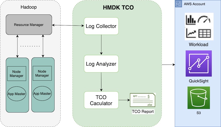
The Hadoop workload insights enable you to design a well-architected EMR cluster to achieve performance and cost-effectiveness in an agile way. For conducting well-architected designs, you need to deliberate between various system specifications of an EMR cluster and multiple cost considerations.
The system specifications are as follows:
- Number of EMR clusters – Amazon EMR enables you to run multiple elastic clusters in the AWS Cloud to serve the same purpose of a shared static Hadoop cluster on premises
- Types of EMR cluster (persistent or transient) – Design your system to keep minimum persistent clusters to save cost
- Instance types and configuration (memory, vCore, and so on) – Choose the right instance for your job
- Resource allocation for applications and cluster utilization – Based on the on-premises workload analysis, design effective resource allocation and efficient resource utilization in future EMR clusters
The cost considerations are as follows:
- Latest price list (from thousands of available EC2 instances available) – The HMDK TCO tool makes the price calculation with Amazon Elastic Compute Cloud (Amazon EC2) instance types, configurations, and their prices.
- Amazon S3 storage cost (standard, Glacier, and so on) – Data replication is no longer required for reliability. You can use tired storage in Amazon S3 for cost savings.
YARN log collector
The HMDK TCO tool enables a simple way to capture Hadoop YARN logs, which include the Hadoop job runs statistics and the corresponding resource usages. The following screenshot is an example of a YARN log.
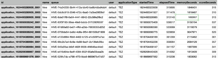
The tool supports HTTPS protocol to communicate with YARN Resource Manager. The tool transports the JSON YARN logs as the inputs to a Python parser, which converts the YARN logs from JSON to CSV format. The new CSV formatted logs are the standard input files for the YARN log analyzer.
For more information, see the GitHub repo.
YARN log analyzer and optimized design use cases
With the log, we can follow up the steps in the TCO yarn-log-analysis README file to use AWS CloudFormation to set up QuickSight resources.
The HMDK TCO log analyzer generates a QuickSight dashboard on various metrics:
- Job timeline – How many jobs are running at one time
- Job user – Breakdown of users and queues
- Application type and engine type – Breakdown by application types (Spark, Hive, Presto) and run engine type (MapReduce, Spark, Tez)
- Elapsed time – The time span of completing an application
- Resources – Memory and CPU
The following screenshot shows an example dashboard.
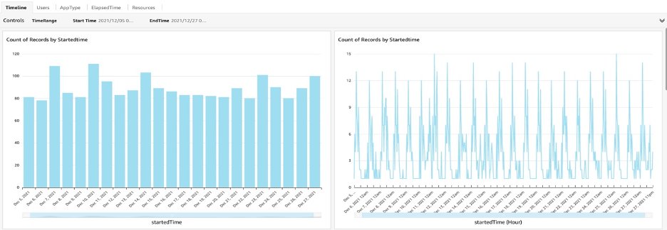
The QuickSight dashboards exhibit insights based on consecutive YARN logs collected in a long-enough period of time (for example, a 2-week window). The insights from the logs reveal the application types, users, queues, running cadence, time spans, and resource usages. The data also helps you discover daily batch jobs or ad hoc jobs, long-running jobs, and resource consumption. These insights help you design the right clusters, such as transient clusters or baseline permanent clusters, and choose the right EC2 instance for memory- or compute-intensive jobs. With the log analyzer results, the TCO tool automatically calculates the TCO of a future EMR cluster.
Let’s see some real customer use cases in the following sections.
Case 1: Use transient and persistent clusters wisely
For this use case, a customer in the financial sector has an 11-node Hadoop cluster.
The QuickSight timeline dashboard shows the peak time job runs because of the daily batch job. This guides us to design two clusters for fulfilling the existing workloads. When we keep a persistent cluster at a minimal size, we can have the transient EMR cluster to handle the batch style job around the peak time.
Therefore, we designed the clusters to have a persistent cluster with 2 data nodes, while transient nodes can scale from 0–10 between the hours of 1:00 AM and 4:00 AM.
The following figure illustrates this design.

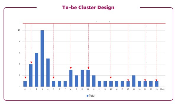
This balanced design using transient and persistent clusters resulted in a cost savings of about 80% compared to a lift-and-shift design.
Case 2: Identify Hadoop queue usage and long-running jobs to design multiple clusters and optimized runs
For our next use case, a company runs 196 nodes using Hadoop 3.1 with jobs like Hive, Spark, and Kafka. The Hadoop default queue and four other queues were used to group various workloads. As illustrated in the following figure, some very long-running jobs are seen in the shared cluster, resulting in queued jobs that have resource competition and unbalanced resource allocation.


The QuickSight user dashboard guides us through the queue usage, the elapsed time dashboard guides us through the long-running jobs, and the resource dashboard guides us through the memory and vCore usage for the jobs.
Therefore, we design a solution to transfer queue jobs to run in separated clusters, and the default queue jobs are split to run in different clusters. By identifying the long-running jobs and understanding the resource needs, we could design a cluster to run such jobs more efficiently.
This design allows the job to run faster and the clusters to be used more efficiently with a cost savings benefit.
Cluster design
The HMDK TCO tool provides a cluster design template like the following example.

Here we have two clusters, one transient and one persistent, to handle the Spark and Tez jobs accordingly. The starting and ending hour for each cluster can be determined from the log analysis. With this cluster design, we can get the hourly workload resource usage forecast. Then the TCO calculator gets all the information needed to generate costs based on the TCO simulation variables you choose.
TCO calculator
The HMDK TCO calculator is a component guiding the EMR cluster design by using the EMR design template. Then it generates the hourly aggregated resource usage forecast using a Python program. The component provides guidelines and an Excel template to input system and cost specification parameters. The component has the logic with a built-in Amazon EMR price list. The 1-year and 3-year TCO cost can be automatically generated by the macro-enabled Excel TCO template.
The following figure shows the details of our HMDK TCO simulation.
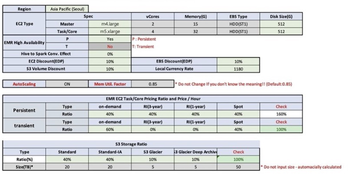
The following figures show the TCO report.

TCO tool engagement outcomes
In this section, we share some of the engagement outcomes from customers after using the TCO tool for 1–2 weeks. Additionally, with the TCO tool, we can refactor on-premises Hadoop clusters to EMR clusters utilizing Amazon S3 as a data lake. The modern data solution of migrating to Amazon EMR provides unlimited scalability with operational efficiency and cost savings.
The following table illustrates four case studies of some engagements using the tool.
| Case# | Case Description | Engagement Outcome |
| 1 | Pressured by the Hadoop License, they migrated to AWS using Amazon EMR and used Spark for replacing Hive. They designed the new EMR clusters using a balanced design of transient and persistent clusters. | They can get job insights through the tool and design the new EMR clusters to fulfill the existing workloads, and expect to achieve 80% cost savings and six times performance enhancement. |
| 2 | Their goal was to migrate a Hadoop cluster with over 1,000 nodes from HDFS to Amazon S3 and Hive to Spark, and redesign the cluster using a balanced design of transient and persistent clusters. | They can get job insights and redesign the cluster with a 1-year TCO of the optimized redesign architecture expected to have 64% cost savings. |
| 3 | Their goal was to migrate to Hadoop 3.1. They transferred the Hadoop queue-based job, which shared the same cluster, to two transient clusters and five persistent clusters with optimized resource usage for each job run, and handled long-running jobs faster. | They can get Amazon EMR TCO results quickly in 2 weeks. Customers get insights on their workloads and long-running jobs and get the job done faster and cheaper. |
| 4 | Their goal was to migrate from Hive 1 to Spark and design an auto scaling EMR cluster. | They can get Amazon EMR TCO results in 1 week. They’re expecting to see 75% cost savings on the redesigned EMR clusters and 10 times on performance improvement. |
Conclusion
This post introduced use cases, functions, and components of the HMDK TCO tool. Through the case studies discussed in this post, you learned about real examples of the tool usage and its benefits. The HMDK TCO tool is designed for automating source Hadoop cluster workload assessment with calculated TCO calculation, and it can be done in 2–3 weeks instead of months.
More and more customers are adopting the HMDK TCO tool to accelerate their migration to Amazon EMR.
To dive deep into the HMDK TCO tool, refer to the next post in this series, How AWS ProServe Hadoop TCO tool accelerate Hadoop workload migrations to Amazon EMR.
About the authors
Sungyoul Park is a Senior Practice Manager at AWS ProServe. He helps customers innovate their business with AWS Analytics, IoT, and AI/ML services. He has a specialty in big data services and technologies and an interest in building customer business outcomes together.
Jiseong Kim is a Senior Data Architect at AWS ProServe. He mainly works with enterprise customers to help data lake migration and modernization, and provides guidance and technical assistance on big data projects such as Hadoop, Spark, data warehousing, real-time data processing, and large-scale machine learning. He also understands how to apply technologies to solve big data problems and build a well-designed data architecture.
George Zhao is a Senior Data Architect at AWS ProServe. He is an experienced analytics leader working with AWS customers to deliver modern data solutions. He is also a ProServe Amazon EMR domain specialist who enables ProServe consultants on best practices and delivery kits for Hadoop to Amazon EMR migrations. His area of interests are data lakes and cloud modern data architecture delivery.
Kalen Zhang was the Global Segment Tech Lead of Partner Data and Analytics at AWS. As a trusted advisor of data and analytics, she curated strategic initiatives for data transformation, led data and analytics workload migration and modernization programs, and accelerated customer migration journeys with partners at scale. She specializes in distributed systems, enterprise data management, advanced analytics, and large-scale strategic initiatives.
Amazon Managed Workflows for Apache Airflow (Amazon MWAA) is a managed orchestration service for Apache Airflow that makes it simple to set up and operate end-to-end data pipelines in the cloud at scale. A data pipeline is a set of tasks and processes used to automate the movement and transformation of data between different systems. The Apache Airflow open-source community provides over 1,000 pre-built operators (plugins that simplify connections to services) for Apache Airflow to build data pipelines. The Amazon provider package for Apache Airflow comes with integrations for over 31 AWS services, such as Amazon Simple Storage Service (Amazon S3), Amazon Redshift, Amazon EMR, AWS Glue, Amazon SageMaker, and more.
The most common use case for Airflow is ETL (extract, transform, and load). Nearly all Airflow users implement ETL pipelines ranging from simple to complex. Operationalizing machine learning (ML) is another growing use case, where data has to be transformed and normalized before it can be loaded into an ML model. In both use cases, the data pipeline is preparing the data for consumption by ingesting data from different sources and transforming it through a series of steps.
Observability across the different processes within the data pipeline is a key component to monitor the success or failure of the pipeline. Although scheduling the runs of tasks within the data pipeline is controlled by Airflow, the run of the task itself (transforming, normalizing, and aggregating data) is done by different services based on the use case. Having an end-to-end view of the data flow is a challenge due to multiple touch points in the data pipeline.
In this post, we provide an overview of logging enhancements when working with Amazon MWAA, which is one of the pillars of observability. We then discuss a solution to further enhance end-to-end observability by modifying the task definitions that make up the data pipeline. For this post, we focus on task definitions for two services: AWS Glue and Amazon EMR, however the same method can be applied across different services.
Challenge
Many customers’ data pipelines start simple, orchestrating a few tasks, and over time grow to be more complex, consisting of a large number of tasks and dependencies between them. As the complexity increases, it becomes increasingly hard to operate and debug in case of failure, which creates a need for a single pane of glass to provide end-to-end data pipeline orchestration and health management. For data pipeline orchestration, the Apache Airflow UI is a user-friendly tool that provides detailed views into your data pipeline. When it comes to pipeline health management, each service that your tasks are interacting with could be storing or publishing logs to different locations, such as an S3 bucket or Amazon CloudWatch logs. As the number of integration touch points increases, stitching the distributed logs generated by different services in various locations can be challenging.
One solution provided by Amazon MWAA to consolidate the Airflow and task logs within the directed acyclic graph (DAG) is to forward the logs to CloudWatch log groups. A separate log group is created for each enabled Airflow logging option (For example, DAGProcessing, Scheduler, Task, WebServer, and Worker). These logs can be queried across log groups using CloudWatch Logs Insights.
A common approach in distributed tracing is to use a correlation ID to stitch and query distributed logs. A correlation ID is a unique identifier that is passed through a request flow for tracking a sequence of activities throughout the lifetime of the workflow. When each service in the workflow needs to log information, it can include this correlation ID, thereby ensuring you can track a full request from start to finish.
The Airflow engine passes a few variables by default that are accessible to all templates. run\_id is one such variable, which is a unique identifier for a DAG run. The run\_id can be used as the correlation ID to query against different log groups within CloudWatch to capture all the logs for a particular DAG run.
However, be aware that services that your tasks are interacting with will use a separate log group and won’t log the run\_id as part of their output. This will prevent you from getting an end-to-end view across the DAG run.
For example, if your data pipeline consists of an AWS Glue task running a Spark job as part of the pipeline, then the Airflow task logs will be available in one CloudWatch log group and the AWS Glue job logs will be in a different CloudWatch log group. However, the Spark job that is run as part of the AWS Glue job doesn’t have access to the correlation ID and can’t be tied back to a particular DAG run. So even if you use the correlation ID to query the different CloudWatch log groups, you won’t get any information about the run of the Spark job.
Solution overview
As you now know, run\_id is a variable that is a unique identifier for a DAG run. The run\_id is present as part of the Airflow task logs. To use the run\_id effectively and increase the observability across the DAG run, we use run\_id as the correlation ID and pass it to different tasks with the DAG. The correlation ID is then be consumed by the scripts used within the tasks.
The following diagram illustrates the solution architecture.

The data pipeline that we focus on consists of the following components:
- An S3 bucket that contains the source data
- An AWS Glue crawler that creates the table metadata in the Data Catalog from the source data
- An AWS Glue job that transforms the raw data into a processed data format while performing file format conversions
- An EMR job that generates reporting datasets
For details on the architecture and complete steps on how to run the DAG refer, to Amazon MWAA for Analytics Workshop.
In the next sections, we explore the following topics:
- The DAG file, in order to understand how to define and then pass the correlation ID in the AWS Glue and EMR tasks
- The code needed in the Python scripts to output information based on the correlation ID
Refer to the GitHub repo for the detailed DAG definition and Spark scripts. To run the scripts, refer to the Amazon MWAA analytics workshop.
DAG definitions
In this section, we look at snippets of the additions needed to the DAG file. We also discuss how to pass the correlation ID to the AWS Glue and EMR jobs. Refer to the GitHub repo for the complete DAG code.
The DAG file begins by defining the variables:
# Variables
Next, let’s look at how to pass the correlation ID to the AWS Glue job using the AWS Glue operator. Operators are the building blocks of Airflow DAGs. They contain the logic of how data is processed in the data pipeline. Each task in a DAG is defined by instantiating an operator.
Airflow provides operators for different tasks. For this post, we use the AWS Glue operator.
The AWS Glue task definition contains the following:
- The Python Spark job script (raw\_to\_tranform.py) to run the job
- The DAG name, task ID, and correlation ID, which are passed as arguments
- The AWS Glue service role assigned, which has permissions to run the crawler and the jobs
See the following code:
# Glue Task definition
Next, we pass the correlation ID to the EMR job using the EMR operator. This includes the following steps:
- Define the configuration of an EMR cluster.
- Create the EMR cluster.
- Define the steps to be run by the EMR job.
- Run the EMR job:
- We use the Python Spark job script aggregations.py.
- We pass the DAG name, task ID, and correlation ID as arguments to the steps for the EMR task.
Let’s start with defining the configuration for the EMR cluster. The correlation\_id is passed in the name of the cluster to easily identify the cluster corresponding to a DAG run. The logs generated by EMR jobs are published to a S3 bucket; the correlation\_id is part of the LogUri as well. See the following code:
# Define the EMR cluster configuration
Now let’s define the task to create the EMR cluster based on the configuration:
# Create the EMR cluster
cluster\_creator = EmrCreateJobFlowOperator( task\_id= emr\_task\_id, job\_flow\_overrides=JOB\_FLOW\_OVERRIDES, aws\_conn\_id=’aws\_default’, emr\_conn\_id=’emr\_default’, dag=dag)Next, let’s define the steps needed to run as part of the EMR job. The input and output data processed by the EMR job is stored in an S3 bucket passed as arguments. Dag\_name, task\_id, and correlation\_id are also passed in as arguments. The task\_id used can be the name of your choice; here we use add\_steps:
# EMR steps to be executed by EMR cluster
Next, let’s add a task to run the steps on the EMR cluster. The job\_flow\_id is the ID of the JobFlow, which is passed down from the EMR create task described earlier using Airflow XComs. See the following code:
#Run the EMR job
This completes the steps needed to pass the correlation ID within the DAG task definition.
In the next section, we use this ID within the script run to log details.
Job script definitions
In this section, we review the changes required to log information based on the correlation\_id. Let’s start with the AWS Glue job script (for the complete code, refer to the following file in GitHub):
# Script changes to file ‘raw\_to\_transform’
Next, we focus on the EMR job script (for the complete code, refer to the file in GitHub):
# Script changes to file ‘nyc\_aggregations’
This completes the steps for passing the correlation ID to the script run.
After we complete the DAG definitions and script additions, we can run the DAG. Logs for a particular DAG run can be queried using the correlation ID. The correlation ID for a DAG run can be found via the Airflow UI. An example of a correlation ID is manual\_\_2022-07-12T00:22:36.111190+00:00. With this unique string, we can run queries on the relevant CloudWatch log groups using CloudWatch Logs Insights. The result of the query includes the logging provided by the AWS Glue and EMR scripts, along with other logs associated with the correlation ID.
Example query for DAG level logs : manual\_\_2022-07-12T00:22:36.111190+00:00
We can also obtain task-level logs by using the format <dag\_name.task\_id correlation\_id>:
Example query : data\_pipeline.glue\_task manual\_\_2022-07-12T00:22:36.111190+00:00
Clean up
If you created the setup to run and test the scripts using the Amazon MWAA analytics workshop, perform the cleanup steps to avoid incurring charges.
Conclusion
In this post, we showed how to send Amazon MWAA logs to CloudWatch log groups. We then discussed how to tie in logs from different tasks within a DAG using the unique correlation ID. The correlation ID can be outputted with as much or as little information needed by your job to provide more details across your entire DAG run. You can then use CloudWatch Logs Insights to query the logs.
With this solution, you can use Amazon MWAA as a single pane of glass for data pipeline orchestration and CloudWatch logs for data pipeline health management. The unique identifier improves the end-to-end observability for a DAG run and helps reduce the time needed for troubleshooting.
To learn more and get hands-on experience, start with the Amazon MWAA analytics workshop and then use the scripts in the GitHub repo to gain more observability of your DAG run.
About the Author
 Payal Singh is a Partner Solutions Architect at Amazon Web Services, focused on the Serverless platform. She is responsible for helping partner and customers modernize and migrate their applications to AWS.
For data lake customers who need to discover petabytes of data, AWS Glue crawlers are a popular way to discover and catalog data in the background. This allows users to search and find relevant data from multiple data sources. Many customers also have data in managed operational databases such as MongoDB Atlas and need to combine it with data from Amazon Simple Storage Service (Amazon S3) data lakes to derive insights. AWS Glue crawlers now support MongoDB Atlas, making it simpler for you to understand MongoDB collections’ evolution and extract meaningful insights.
AWS Glue is a serverless data integration service that makes it simple to discover, prepare, move, and integrate data from multiple sources for analytics, machine learning (ML), and application development.
MongoDB Atlas is a developer data service from AWS technology partner MongoDB, Inc. The service combines transactional processing, relevance-based search, real-time analytics, and mobile-to-cloud data synchronization in an integrated architecture.
With today’s launch, you can create and schedule an AWS Glue crawler to crawl MongoDB Atlas. In the crawler setup, you can select MongoDB as a data source. You can then create an AWS Glue connection with MongoDB Atlas and provide the MongoDB Atlas cluster name and credentials. We walk you through this process in this post.
Solution overview
The following architecture illustrates how you can scan a MongoDB Atlas database and collections using AWS Glue.

With each run of the crawler, the crawler inspects specified collections and catalogs information, such as updates or deletes to MongoDB Atlas collections, views, and materialized views in the AWS Glue Data Catalog. In AWS Glue Studio, you can then use the AWS Glue Data Catalog as a source to pull data from MongoDB Atlas and populate an Amazon S3 target. Finally, this job can run and read data from MongoDB Atlas and write the results to Amazon S3, opening up possibilities to integrate with AWS services such as Amazon SageMaker, Amazon QuickSight, and more.
In the following sections, we describe how to create an AWS Glue crawler with MongoDB Atlas as a data source. We then create an AWS Glue connection and provide the MongoDB Atlas cluster information and credentials. Then we specify the MongoDB Atlas database and collections to crawl.
Prerequisites
To follow along with this post, you must have access to MongoDB Atlas and the AWS Management Console. We also assume you have access to a VPC with subnets preconfigured via Amazon Virtual Private Cloud (Amazon VPC). The crawler that we configure later in the post runs in the VPC and connects to MongoDB Atlas via an AWS PrivateLink endpoint.
Set up MongoDB Atlas
To configure MongoDB Atlas, complete the following steps:
- Configure a MongoDB cluster on AWS. For instructions, refer to How to Set Up a MongoDB Cluster.
- Configure PrivateLink by following the steps described in Connecting Applications Securely to a MongoDB Atlas Data Plane with AWS PrivateLink.
This allows us to simplify our networking architecture and make sure the traffic stays on the AWS network.
Next, we obtain the MongoDB cluster connection string from the Connect UI on the MongoDB Atlas console.
- On the MongoDB Atlas console, choose Connect, Private Endpoint, and Connection Method.
- Copy the SRV connection string.

We use this SRV connection string in the subsequent steps.
The following screenshot shows that we have loaded a sample collection in MongoDB Atlas, which we crawl over in the next steps. Note that the records in this collection include several arrays as well as nested data.

Set up the MongoDB Atlas connection with AWS Glue
Before we can configure the AWS Glue crawler, we need to create the MongoDB Atlas connection in AWS Glue.
- On the AWS Glue Studio console, choose Connectors in the navigation pane.
- Choose Create connection.

- When filling out the connection details, use the SRV connection string we obtained earlier in MongoDB Atlas.
- In the Network options section, the VPC and subnets must correspond to the PrivateLink settings you configured earlier.

Create a MongoDB crawler
After we create the connection, we can create an AWS Glue crawler.
- On the AWS Glue console, choose Crawlers in the navigation pane.
- Choose Create crawler.

- For Name, enter a name.
- For the data source, choose the MongoDB Atlas data source we configured earlier and supply the path that corresponds to the MongoDB Atlas database and collection.

- Configure your security settings, output, and scheduling.

- On the Crawlers page, choose Run crawler.

After the crawler finishes crawling the MongoDB collections, its status shows as Completed.
Review the MongoDB AWS Glue database and table
We can navigate to the AWS Glue Data Catalog to examine the tables that were created by the crawler.

Choose the table to view the schema and other metadata.

Note that the crawler captured nested data as a STRUCT and correctly listed the ARRAY fields.
Import MongoDB Atlas data to Amazon S3
Now we use the MongoDB Atlas-based AWS Glue Data Catalog table to perform a data import without writing code. We use AWS Glue Studio to build boilerplate code quickly. Alternatively, you can build the script in script editor.
- On the AWS Glue Studio console, choose Jobs in the navigation pane.
- Choose Create job.
- Select Visual with a source and target.
- Choose the Data Catalog table as the source and Amazon S3 as the target.

- In the AWS Glue Studio UI, supply additional parameters such as the S3 bucket name and choose the database and table from the drop-down menus.

- Next, review the generated script that is built by AWS Glue Studio. We now need to add a database and collection in the script as follows:

When the ETL job is complete, the extracted data is available on Amazon S3.
- On the Amazon S3 console, choose Buckets in the navigation pane.
- Choose our bucket and folder containing the extracted files.
- Choose a file and on the Actions menu, choose Query with S3 Select to view the contents of the file.

Clean up
To avoid incurring charges for the services used in this walkthrough, complete the following steps to delete your resources:
- On the AWS Glue console, choose Crawlers in the navigation pane.
- Select your crawler and on the Action menu, choose Delete crawler.
- On the AWS Glue Studio console, choose View jobs.
- Select the job you created and on the Actions menu, choose Delete job(s).
- Return to the AWS Glue console and choose Tables in the navigation pane.
- Select your table and choose Delete.
- Choose Databases in the navigation pane.
- Select your database and choose Delete.
- On the Amazon VPC console, choose Endpoints in the navigation pane.
- Select the PrivateLink endpoint you created and on the Actions menu, choose Delete VPC endpoints.
Conclusion
In this post, we showed how to set up an AWS Glue crawler to crawl over a MongoDB Atlas collection, gathering metadata and creating table records in the AWS Glue Data Catalog. With the Data Catalog table, we created an ETL process using the AWS Glue Studio UI to extract data from the MongoDB Atlas collection to an S3 bucket without writing a single line of code.
You can try this yourself by configuring an AWS Glue crawler, creating an AWS Glue ETL job with AWS Glue Studio, and launching MongoDB Atlas from a QuickStart or from MongoDB Atlas on AWS Marketplace.
Special thanks to everyone who contributed to this crawler feature launch: Julio Montes de Oca, Mita Gavade, and Alex Prazma.
About the authors
Igor Alekseev is a Senior Partner Solution Architect at AWS in Data and Analytics domain. In his role Igor is working with strategic partners helping them build complex, AWS-optimized architectures. Prior joining AWS, as a Data/Solution Architect he implemented many projects in Big Data domain, including several data lakes in Hadoop ecosystem. As a Data Engineer he was involved in applying AI/ML to fraud detection and office automation.
Sandeep Adwankar is a Senior Technical Product Manager at AWS. Based in the California Bay Area, he works with customers around the globe to translate business and technical requirements into products that enable customers to improve how they manage, secure, and access data.
Since its launch in 2006, Amazon Simple Storage Service (Amazon S3) has experienced major growth, supporting multiple use cases such as hosting websites, creating data lakes, serving as object storage for consumer applications, storing logs, and archiving data. As the application portfolio grows, customers tend to store data from multiple application and different business functions in a single S3 bucket, which can grow the storage in S3 buckets to hundreds of TBs. The AWS Billing console provides a way to look at the total storage cost of data stored in Amazon S3, but sometimes IT organizations need to understand the breakdown of costs of a particular S3 bucket by various prefixes or objects corresponding to a particular user or application. There are various reasons to analyze the costs of S3 buckets, such as to identify the spend breakdown, do internal chargebacks, understand the cost breakdown by business unit and application, and many more. As of this writing, there is no easy way to do a cost breakdown of S3 buckets by objects and prefixes.
In this post, we discuss a solution using Amazon Athena to query AWS Cost and Usage Reports and Amazon S3 Inventory reports to analyze the cost by prefixes and objects in an S3 bucket.
Overview of solution
The following figure shows the architecture for this solution. First, we enable the AWS Cost and Usage Reports (AWS CUR) and Amazon S3 Inventory features, which save the output into two separate pre-created S3 buckets. We then use Athena to query these S3 buckets for AWS CUR data and S3 object inventory data to correlate and allocate the cost breakdown at the object or prefix level.

To implement the solution, we complete the following steps:
- Create S3 buckets for AWS CUR, S3 object inventory, and Athena results. Alternatively, you can create these respective buckets when enabling the respective individual features, but for the purpose of this post, we create all of them at the beginning.
- Enable the Cost and Usage Reports.
- Enable Amazon S3 Inventory configuration.
- Create AWS Glue Data Catalog tables for the CUR and S3 object inventory to query using Athena.
- Run queries in Athena.
Prerequisites
For this walkthrough, you should have the following prerequisites:
- An AWS account.
- AWS Identity and Access Management (IAM) permissions for the following services:
- Amazon S3 – Create and manage S3 buckets.
- AWS Billing and Cost Management – Create Cost and Usage Reports.
- Athena – Create tables and run queries. AWS Glue Data Catalog permissions are needed to create tables.
Create S3 buckets
Amazon S3 is an object storage service offering industry-leading scalability, data availability, security, and performance. Customers of all sizes and industries can store and protect any amount of data for virtually any use case, such as data lakes, cloud-native applications, and mobile apps. With cost-effective storage classes and easy-to-use management features, you can optimize costs, organize data, and configure fine-tuned access controls to meet specific business, organizational, and compliance requirements.
For this post, we use the S3 bucket s3-object-cost-allocation as the primary bucket for cost allocation. This S3 bucket is conveniently modeled to contain several prefixes and objects of different sizes for which cost allocation needs to be done based on the overall cost of the bucket. In a real-world scenario, you should use a bucket that has data for multiple teams and for which you need to allocate costs by prefix or object. Going forward, we refer to this bucket as the primary object bucket.
The following screenshot shows our S3 bucket and folders.

Now let’s create the three additional operational S3 buckets to store the datasets generated to calculate costs for the objects. You can create the following buckets or any existing buckets as needed:
cur-cost-usage-reports-<account\_number>– This bucket is used to save the Cost and Usage Reports for the account.S3-inventory-configurations-<account\_number>– This bucket is used to save the inventory configurations of our primary object bucket.athena-query-bucket-<account\_number>– This bucket is used to save the query results from Athena.
Complete the following steps to create your S3 buckets:
- On the Amazon S3 console, choose Buckets in the navigation pane.
- Choose Create bucket.
- For Bucket name, enter the name of your bucket (
cur-cost-usage-reports-<account\_number>). - For AWS Region, choose your preferred Region.
- Leave all other settings at default (or according to your organization’s standards).
- Choose Create bucket.

- Repeat these steps to create
s3-inventory-configurations-<account\_number>andathena-query-bucket-<account\_number>.
Enable the Cost and Usage Reports
The AWS Cost and Usage Reports (AWS CUR) contains the most comprehensive set of cost and usage data available. You can use Cost and Usage Reports to publish your AWS billing reports to an S3 bucket that you own. You can receive reports that break down your costs by the hour, day, or month; by product or product resource; or by tags that you define yourself.
Complete the following steps to enable Cost and Usage Reports for your account:
- On the AWS Billing console, in the navigation pane, choose Cost & Usage Reports.
- Choose Create report.
- For Report name, enter a name for your report, such as
account-cur-s3. - For Additional report details, select Include resource IDs to include the IDs of each individual resource in the report.Including resource IDs will create individual line items for each of your resources. This can increase the size of your Cost and Usage Reports files significantly, which can affect the S3 storage costs for your CUR, based on your AWS usage. We need this feature enabled for this post.
- For Data refresh settings, select whether you want the Cost and Usage Reports to refresh if AWS applies refunds, credits, or support fees to your account after finalizing your bill.When a report refreshes, a new report is uploaded to Amazon S3.
- Choose Next.
- For S3 bucket, choose Configure.
- For Configure S3 Bucket, select an existing bucket created in the previous section (
cur-cost-usage-reports-<account\_number>) and choose Next. - Review the bucket policy, select I have confirmed that this policy is correct, and choose Save. This default bucket policy provides Cost and Usage Reports access to write data to Amazon S3.
- For Report path prefix, enter
cur-data/account-cur-daily. - For Time granularity, choose Daily.
- For Report versioning, choose Overwrite existing report.
- For Enable report data integration for, select Amazon Athena.
- Choose Next.
- After you have reviewed the settings for your report, choose Review and Complete.

The Cost and Usage reports will be delivered to the S3 buckets within 24 hours.
The following sample CUR in CSV format shows different columns of the Cost and Usage Report, including bill\_invoice\_id, bill\_invoicing\_entity, bill\_payer\_account\_id, and line\_item\_product\_code, to name a few.

Enable Amazon S3 Inventory configuration
Amazon S3 Inventory is one of the tools Amazon S3 provides to help manage your storage. You can use it to audit and report on the replication and encryption status of your objects for business, compliance, and regulatory needs. Amazon S3 Inventory provides comma-separated values (CSV), Apache Optimized Row Columnar (ORC), or Apache Parquet output files that list your objects and their corresponding metadata on a daily or weekly basis for an S3 bucket or a shared prefix (objects that have names that begin with a common string).
Complete the following steps to enable Amazon S3 Inventory on the primary object bucket:
- On the Amazon S3 console, choose Buckets in the navigation pane.
- Choose the bucket for which you want to configure Amazon S3 Inventory.
This will be the existing bucket in your account that has data that needs to be analyzed. This could be your data lake or application S3 bucket. We created the buckets3-object-cost-allocationwith some sample data and folder structure. - Choose Management.
- Under Inventory configurations, choose Create inventory configuration.
- For Inventory configuration name, enter
s3-object-cost-allocation. - For Inventory scope, leave Prefix blank.
This is to ensure that all objects are covered for the report. - For Object Versions, select Current version only.
- For Report details, choose This account.
- For Destination, choose the destination bucket we created (
s3-inventory-configurations-<account\_number>). - For Frequency, choose Daily.
- For Output format, choose as Apache Parquet.
- For Status, choose Enable.
- Keep server-side encryption disabled. To use server-side encryption, choose Enable and specify the encryption key.
- For Additional fields, select the following to add to the inventory report:
- Size – The object size in bytes.
- Last modified date – The object creation date or the last modified date, whichever is the latest.
- Multipart upload – Specifies that the object was uploaded as a multipart upload. For more information, see Uploading and copying objects using multipart upload.
- Replication status – The replication status of the object. For more information, see Using the S3 console.
- Encryption status – The server-side encryption used to encrypt the object. For more information, see Protecting data using server-side encryption.
- Bucket key status – Indicates whether a bucket-level key generated by AWS KMS applies to the object.
- Storage class – The storage class used for storing the object.
- Intelligent-Tiering: Access tier – Indicates the access tier of the object if it was stored in Intelligent-Tie

- Choose Create.

It may take up to 48 hours to deliver the first report.
Create AWS Glue Data Catalog tables for CUR and Amazon S3 Inventory reports
Wait for up to 48 hours for the previous step to generate the reports. In this section, we use Athena to create and define AWS Glue Data Catalog tables for the data that has been created using Cost and Usage Reports and Amazon S3 Inventory reports.
Athena is a serverless, interactive analytics service built on open-source frameworks, supporting open-table and file formats. Athena provides a simplified, flexible way to analyze petabytes of data where it lives.
Complete the following steps to create the tables using Athena:
- Navigate to the Athena console.
- If you’re using Athena for the first time, you need to set up a query result location in Amazon S3. If you preconfigured this in Athena , you can skip this step.
- Choose View settings.

- Choose Manage.
- In the section Query result location and encryption, choose Browse S3 and choose the bucket that we created (
athena-query-bucket-<account\_number>). - Choose Save.

- Navigate back to the Athena query editor.
- Choose View settings.
- Run the following query in Athena to create a table for Cost and Usage Reports. Verify and update the section for <<LOCATION>> at the end of the query and point it to the correct S3 bucket and location. Note that the new table name should be
account\_cur.CREATE EXTERNAL TABLE `account\_cur`(`identity\_line\_item\_id` string,`identity\_time\_interval` string,`bill\_invoice\_id` string,`bill\_billing\_entity` string,`bill\_bill\_type` string,`bill\_payer\_account\_id` string,`bill\_billing\_period\_start\_date` timestamp,`bill\_billing\_period\_end\_date` timestamp,`line\_item\_usage\_account\_id` string,`line\_item\_line\_item\_type` string,`line\_item\_usage\_start\_date` timestamp,`line\_item\_usage\_end\_date` timestamp,`line\_item\_product\_code` string,`line\_item\_usage\_type` string,`line\_item\_operation` string,`line\_item\_availability\_zone` string,`line\_item\_resource\_id` string,`line\_item\_usage\_amount` double,`line\_item\_normalization\_factor` double,`line\_item\_normalized\_usage\_amount` double,`line\_item\_currency\_code` string,`line\_item\_unblended\_rate` string,`line\_item\_unblended\_cost` double,`line\_item\_blended\_rate` string,`line\_item\_blended\_cost` double,`line\_item\_line\_item\_description` string,`line\_item\_tax\_type` string,`line\_item\_legal\_entity` string,`product\_product\_name` string,`product\_availability` string,`product\_description` string,`product\_durability` string,`product\_event\_type` string,`product\_fee\_code` string,`product\_fee\_description` string,`product\_free\_query\_types` string,`product\_from\_location` string,`product\_from\_location\_type` string,`product\_from\_region\_code` string,`product\_group` string,`product\_group\_description` string,`product\_location` string,`product\_location\_type` string,`product\_message\_delivery\_frequency` string,`product\_message\_delivery\_order` string,`product\_operation` string,`product\_platopricingtype` string,`product\_product\_family` string,`product\_queue\_type` string,`product\_region` string,`product\_region\_code` string,`product\_servicecode` string,`product\_servicename` string,`product\_sku` string,`product\_storage\_class` string,`product\_storage\_media` string,`product\_to\_location` string,`product\_to\_location\_type` string,`product\_to\_region\_code` string,`product\_transfer\_type` string,`product\_usagetype` string,`product\_version` string,`product\_volume\_type` string,`pricing\_rate\_code` string,`pricing\_rate\_id` string,`pricing\_currency` string,`pricing\_public\_on\_demand\_cost` double,`pricing\_public\_on\_demand\_rate` string,`pricing\_term` string,`pricing\_unit` string,`reservation\_amortized\_upfront\_cost\_for\_usage` double,`reservation\_amortized\_upfront\_fee\_for\_billing\_period` double,`reservation\_effective\_cost` double,`reservation\_end\_time` string,`reservation\_modification\_status` string,`reservation\_normalized\_units\_per\_reservation` string,`reservation\_number\_of\_reservations` string,`reservation\_recurring\_fee\_for\_usage` double,`reservation\_start\_time` string,`reservation\_subscription\_id` string,`reservation\_total\_reserved\_normalized\_units` string,`reservation\_total\_reserved\_units` string,`reservation\_units\_per\_reservation` string,`reservation\_unused\_amortized\_upfront\_fee\_for\_billing\_period` double,`reservation\_unused\_normalized\_unit\_quantity` double,`reservation\_unused\_quantity` double,`reservation\_unused\_recurring\_fee` double,`reservation\_upfront\_value` double,`savings\_plan\_total\_commitment\_to\_date` double,`savings\_plan\_savings\_plan\_a\_r\_n` string,`savings\_plan\_savings\_plan\_rate` double,`savings\_plan\_used\_commitment` double,`savings\_plan\_savings\_plan\_effective\_cost` double,`savings\_plan\_amortized\_upfront\_commitment\_for\_billing\_period` double,`savings\_plan\_recurring\_commitment\_for\_billing\_period` double,`resource\_tags\_user\_bucket\_name` string,`resource\_tags\_user\_cost\_tracking` string)PARTITIONED BY (`year` string,`month` string)ROW FORMAT SERDE'org.apache.hadoop.hive.ql.io.parquet.serde.ParquetHiveSerDe'STORED AS INPUTFORMAT'org.apache.hadoop.mapred.TextInputFormat'OUTPUTFORMAT'org.apache.hadoop.hive.ql.io.HiveIgnoreKeyTextOutputFormat'LOCATION'<<LOCATION>>' - Run the following query in Athena to create the table for Amazon S3 Inventory. Verify and update the section for <<LOCATION>> at the end of the query and point it to the correct S3 bucket and location.
- To get the exact value of the location, navigate to the bucket where inventory configurations are stored and navigate to the folder path
Hive. Use the S3 URI to replace <<LOCATION>> in the query.
CREATE EXTERNAL TABLE s3\_object\_inventory( bucket string, key string, version\_id string, is\_latest boolean, is\_delete\_marker boolean, size bigint, last\_modified\_date bigint, storage\_class string, is\_multipart\_uploaded boolean, replication\_status string, encryption\_status string, intelligent\_tiering\_access\_tier string, bucket\_key\_status string) PARTITIONED BY ( dt string)ROW FORMAT SERDE 'org.apache.hadoop.hive.ql.io.parquet.serde.ParquetHiveSerDe' STORED AS INPUTFORMAT 'org.apache.hadoop.hive.ql.io.SymlinkTextInputFormat' OUTPUTFORMAT 'org.apache.hadoop.hive.ql.io.IgnoreKeyTextOutputFormat' LOCATION '<<LOCATION>>';
- To get the exact value of the location, navigate to the bucket where inventory configurations are stored and navigate to the folder path
- We need to refresh the partitions and add new inventory lists to the table. Use the following commands to add data to the CUR table and Amazon S3 Inventory table:
MSCK REPAIR TABLE `account\_cur`;MSCK REPAIR TABLE s3\_object\_inventory;
Run queries in Athena to allocate the cost of objects in an S3 bucket
Now we can query the data we have available to get a cost allocation breakdown at the prefix level.
We need to provide some information in the following queries:
- Update <<YYYY-MM-DD>> with the date for which you want to analyze the data
- Update <<prefix>> with the prefix values for your bucket that needs to be analyzed
- Update <<bucket\_name>> with the name of the bucket that needs to be analyzed
We use the following part of the query to calculate the size of storage being used by the target prefix that we want to calculate the cost for:
select date\_parse(dt,'%Y-%m-%d-%H-%i') dt, cast (sum(size) as double) targetPrefixBytesfrom s3\_object\_inventorywhere date\_parse(dt,'%Y-%m-%d-%H-%i') = cast('<<YYYY-MM-DD>>' as timestamp)and key like '<<prefix>>/%'group by dtNext, we calculate the total size of the bucket on that particular date:
select date\_parse(dt,'%Y-%m-%d-%H-%i') dt, cast (sum(size) as double) totalBytesfrom s3\_object\_inventorywhere date\_parse(dt,'%Y-%m-%d-%H-%i') = cast('<<YYYY-MM-DD>>' as timestamp)group by dtWe query the CUR table to get the cost of a particular bucket on a particular date:
select line\_item\_usage\_start\_date as dt, sum(line\_item\_blended\_cost) as line\_item\_blended\_costfrom "account\_cur"where line\_item\_product\_code = 'AmazonS3'and product\_servicecode = 'AmazonS3'and line\_item\_operation = 'StandardStorage'and line\_item\_resource\_id = '<<bucket\_name>>'and line\_item\_usage\_start\_date = cast('<<YYYY-MM-DD>>' as timestamp)group by line\_item\_usage\_start\_datePutting all of this together, we can calculate the cost of a particular prefix (folder or a file) on a specific date. The complete query is as follows:
withcost as (select line\_item\_usage\_start\_date as dt, sum(line\_item\_blended\_cost) as line\_item\_blended\_costfrom "account\_cur"where line\_item\_product\_code = 'AmazonS3'and product\_servicecode = 'AmazonS3'and line\_item\_operation = 'StandardStorage'and line\_item\_resource\_id = '<<bucket\_name>>'and line\_item\_usage\_start\_date = cast('<<YYYY-MM-DD>>' as timestamp)group by line\_item\_usage\_start\_date),total as (select date\_parse(dt,'%Y-%m-%d-%H-%i') dt, cast (sum(size) as double) totalBytesfrom s3\_object\_inventorywhere date\_parse(dt,'%Y-%m-%d-%H-%i') = cast('<<YYYY-MM-DD>>' as timestamp)group by dt),target as (select date\_parse(dt,'%Y-%m-%d-%H-%i') dt, cast (sum(size) as double) targetPrefixBytesfrom s3\_object\_inventorywhere date\_parse(dt,'%Y-%m-%d-%H-%i') = cast('<<YYYY-MM-DD>>' as timestamp)and key like '<<prefix>>/%'group by dt)select target.dt,(target.targetPrefixBytes/ total.totalBytes * 100) percentUsed,cost.line\_item\_blended\_cost totalCost,cost.line\_item\_blended\_cost*(target.targetPrefixBytes/ total.totalBytes) as prefixCostfrom target, total, costwhere target.dt = total.dtand target.dt = cost.dtThe following screenshot shows the results table for the sample data we used in this post. We get the following information:
- dt – Date
- percentUsed – The percentage of prefix space compared to overall bucket space
- totalCost – The total cost of the bucket
- prefixCost – The cost of the space used by the prefix

Clean up
To stop incurring costs, be sure to disable Amazon S3 Inventory and Cost and Usage Reports when you’re done.
Delete the S3 buckets created for the Amazon S3 Inventory reports and Cost and Usage Reports to avoid storage charges.
Other methods for Amazon S3 storage analysis
Amazon S3 Storage Lens can provide a single view of object storage usage and activity across your entire Amazon S3 storage. With S3 Storage Lens, you can understand, analyze, and optimize storage with over 29 usage and activity metrics and interactive dashboards to aggregate data for your entire organization, specific accounts, Regions, buckets, or prefixes. All of this data is accessible on the Amazon S3 console or as raw data in an S3 bucket.
S3 Storage Lens doesn’t provide cost analysis based on an object or prefix in a single bucket. If you want visibility of storage usage and trends across the entire storage footprint along with recommendations on cost efficiency and data protection best practices, S3 Storage Lens is the right option. But if you want a cost analysis of specific S3 buckets and looking for ways to get cost allocation of S3 objects at the object or prefix level, the solution in this post would be the best fit.
Conclusion
In this post, we detailed how to create a cost breakdown model at the object or prefix level for S3 buckets that contains data for multiple business units and applications. We used Athena to query the reports and datasets produced by the AWS CUR and Amazon S3 Inventory features that, when correlated, give us the cost allocation at the object and prefix level. This solution gives you an easy way to calculate costs for independent objects and prefixes, which can be used for internal chargebacks or just to know the per-object or per-prefix spending in a shared S3 bucket.
About the Authors
 Dagar Katyal is a Senior Solutions Architect at AWS, based in Chicago, Illinois. He works with customers and provides guidance for key strategic initiatives important for their business. Dagar has an MBA and has spent years over 15 years working with customers on projects on analytics strategy, roadmap, and using data as a key differentiator. When not working with customers, Dagar spends time with his family and doing home improvement projects.
 Saiteja Pudi is a Solutions Architect at AWS, based in Dallas, Tx. He has been with AWS for more than 3 years now, helping customers derive the true potential of AWS by being their trusted advisor. He comes from an application development background, interested in Data Science and Machine Learning.
Every day, Amazon devices process and analyze billions of transactions from global shipping, inventory, capacity, supply, sales, marketing, producers, and customer service teams. This data is used in procuring devices’ inventory to meet Amazon customers’ demands. With data volumes exhibiting a double-digit percentage growth rate year on year and the COVID pandemic disrupting global logistics in 2021, it became more critical to scale and generate near-real-time data.
This post shows you how we migrated to a serverless data lake built on AWS that consumes data automatically from multiple sources and different formats. Furthermore, it created further opportunities for our data scientists and engineers to use AI and machine learning (ML) services to continuously feed and analyze data.
Challenges and design concerns
Our legacy architecture primarily used Amazon Elastic Compute Cloud (Amazon EC2) to extract the data from various internal heterogeneous data sources and REST APIs with the combination of Amazon Simple Storage Service (Amazon S3) to load the data and Amazon Redshift for further analysis and generating the purchase orders.
We found this approach resulted in a few deficiencies and therefore drove improvements in the following areas:
- Developer velocity – Due to the lack of unification and discovery of schema, which are primary reasons for runtime failures, developers often spent time dealing with operational and maintenance issues.
- Scalability – Most of these datasets are shared across the globe. Therefore, we must meet the scaling limits while querying the data.
- Minimal infrastructure maintenance – The current process spans multiple computes depending on the data source. Therefore, reducing infrastructure maintenance is critical.
- Responsiveness to data source changes – Our current system gets data from various heterogeneous data stores and services. Any updates to those services takes months of developer cycles. The response times for these data sources are critical to our key stakeholders. Therefore, we must take a data-driven approach to select a high-performance architecture.
- Storage and redundancy – Due to the heterogeneous data stores and models, it was challenging to store the different datasets from various business stakeholder teams. Therefore, having versioning along with incremental and differential data to compare will provide a remarkable ability to generate more optimized plans
- Fugitive and accessibility – Due to the volatile nature of logistics, a few business stakeholder teams have a requirement to analyze the data on demand and generate the near-real-time optimal plan for the purchase orders. This introduces the need for both polling and pushing the data to access and analyze in near-real time.
Implementation strategy
Based on these requirements, we changed strategies and started analyzing each issue to identify the solution. Architecturally, we chose a serverless model, and the data lake architecture action line refers to all the architectural gaps and challenging features we determined were part of the improvements. From an operational standpoint, we designed a new shared responsibility model for data ingestion using AWS Glue instead of internal services (REST APIs) designed on Amazon EC2 to extract the data. We also used AWS Lambda for data processing. Then we chose Amazon Athena as our query service. To further optimize and improve the developer velocity for our data consumers, we added Amazon DynamoDB as a metadata store for different data sources landing in the data lake. These two decisions drove every design and implementation decision we made.
The following diagram illustrates the architecture

In the following sections, we look at each component in the architecture in more detail as we move through the process flow.
AWS Glue for ETL
To meet customer demand while supporting the scale of new businesses’ data sources, it was critical for us to have a high degree of agility, scalability, and responsiveness in querying various data sources.
AWS Glue is a serverless data integration service that makes it easy for analytics users to discover, prepare, move, and integrate data from multiple sources. You can use it for analytics, ML, and application development. It also includes additional productivity and DataOps tooling for authoring, running jobs, and implementing business workflows.
With AWS Glue, you can discover and connect to more than 70 diverse data sources and manage your data in a centralized data catalog. You can visually create, run, and monitor extract, transform, and load (ETL) pipelines to load data into your data lakes. Also, you can immediately search and query cataloged data using Athena, Amazon EMR, and Amazon Redshift Spectrum.
AWS Glue made it easy for us to connect to the data in various data stores, edit and clean the data as needed, and load the data into an AWS-provisioned store for a unified view. AWS Glue jobs can be scheduled or called on demand to extract data from the client’s resource and from the data lake.
Some responsibilities of these jobs are as follows:
- Extracting and converting a source entity to data entity
- Enrich the data to contain year, month, and day for better cataloging and include a snapshot ID for better querying
- Perform input validation and path generation for Amazon S3
- Associate the accredited metadata based on the source system
Querying REST APIs from internal services is one of our core challenges, and considering the minimal infrastructure, we wanted to use them in this project. AWS Glue connectors assisted us in adhering to the requirement and goal. To query data from REST APIs and other data sources, we used PySpark and JDBC modules.
AWS Glue supports a wide variety of connection types. For more details, refer to Connection Types and Options for ETL in AWS Glue.
S3 bucket as landing zone
We used an S3 bucket as the immediate landing zone of the extracted data, which is further processed and optimized.
Lambda as AWS Glue ETL Trigger
We enabled S3 event notifications on the S3 bucket to trigger Lambda, which further partitions our data. The data is partitioned on InputDataSetName, Year, Month, and Date. Any query processor running on top of this data will scan only a subset of data for better cost and performance optimization. Our data can be stored in various formats, such as CSV, JSON, and Parquet.
The raw data isn’t ideal for most of our use cases to generate the optimal plan because it often has duplicates or incorrect data types. Most importantly, the data is in multiple formats, but we quickly modified the data and observed significant query performance gains from using the Parquet format. Here, we used one of the performance tips in Top 10 performance tuning tips for Amazon Athena.
AWS Glue jobs for ETL
We wanted better data segregation and accessibility, so we chose to have a different S3 bucket to improve performance further. We used the same AWS Glue jobs to further transform and load the data into the required S3 bucket and a portion of extracted metadata into DynamoDB.
DynamoDB as metadata store
Now that we have the data, various business stakeholders further consume it. This leaves us with two questions: which source data resides on the data lake and what version. We chose DynamoDB as our metadata store, which provides the latest details to the consumers to query the data effectively. Every dataset in our system is uniquely identified by snapshot ID, which we can search from our metadata store. Clients access this data store with an API’s.
Amazon S3 as data lake
For better data quality, we extracted the enriched data into another S3 bucket with the same AWS Glue job.
AWS Glue Crawler
Crawlers are the “secret sauce” that enables us to be responsive to schema changes. Throughout the process, we chose to make each step as schema-agnostic as possible, which allows any schema changes to flow through until they reach AWS Glue. With a crawler, we could maintain the agnostic changes happening to the schema. This helped us automatically crawl the data from Amazon S3 and generate the schema and tables.
AWS Glue Data Catalog
The Data Catalog helped us maintain the catalog as an index to the data’s location, schema, and runtime metrics in Amazon S3. Information in the Data Catalog is stored as metadata tables, where each table specifies a single data store.
Athena for SQL queries
Athena is an interactive query service that makes it easy to analyze data in Amazon S3 using standard SQL. Athena is serverless, so there is no infrastructure to manage, and you pay only for the queries you run. We considered operational stability and increasing developer velocity as our key improvement factors.
We further optimized the process to query Athena so that users can plug in the values and the queries to get data out of Athena by creating the following:
- An AWS Cloud Development Kit (AWS CDK) template to create Athena infrastructure and AWS Identity and Access Management (IAM) roles to access data lake S3 buckets and the Data Catalog from any account
- A library so that client can provide an IAM role, query, data format, and output location to start an Athena query and get the status and result of the query run in the bucket of their choice.
To query Athena is a two-step process:
- StartQueryExecution – This starts the query run and gets the run ID. Users can provide the output location where the output of the query will be stored.
- GetQueryExecution – This gets the query status because the run is asynchronous. When successful, you can query the output in an S3 file or via API.
The helper method for starting the query run and getting the result would be in the library.
Data lake metadata service
This service is custom developed and interacts with DynamoDB to get the metadata (dataset name, snapshot ID, partition string, timestamp, and S3 link of the data) in the form of a REST API. When the schema is discovered, clients use Athena as their query processor to query the data.
Because all datasets have a snapshot ID are partitioned, the join query doesn’t result in a full table scan but only a partition scan on Amazon S3. We used Athena as our query processor because of its ease in not managing our query infrastructure. Later, if we feel we need something more, we can use either Redshift Spectrum or Amazon EMR.
Conclusion
Amazon Devices teams discovered significant value by moving to a data lake architecture using AWS Glue, which enabled multiple global business stakeholders to ingest data in more productive ways. This enabled the teams to generate the optimal plan to place purchase orders for devices by analyzing the different datasets in near-real time with appropriate business logic to solve the problems of the supply chain, demand, and forecast.
From an operational perspective, the investment has already started to pay off:
- It standardized our ingestion, storage, and retrieval mechanisms, saving onboarding time. Before the implementation of this system, one dataset took 1 month to onboard. Due to our new architecture, we were able to onboard 15 new datasets in less than 2 months, which improved our agility by 70%.
- It removed scaling bottlenecks, creating a homogeneous system that can quickly scale to thousands of runs.
- The solution added schema and data quality validation before accepting any inputs and rejecting them if data quality violations are discovered.
- It made it easy to retrieve datasets while supporting future simulations and back tester use cases requiring versioned inputs. This will make launching and testing models simpler.
- The solution created a common infrastructure that can be easily extended to other teams across DIAL having similar issues with data ingestion, storage, and retrieval use cases.
- Our operating costs have fallen by almost 90%.
- This data lake can be accessed efficiently by our data scientists and engineers to perform other analytics and have a predictive approach as a future opportunity to generate accurate plans for the purchase orders.
The steps in this post can help you plan to build a similar modern data strategy using AWS-managed services to ingest data from different sources, automatically create metadata catalogs, share data seamlessly between the data lake and data warehouse, and create alerts in the event of an orchestrated data workflow failure.
About the authors
 Avinash Kolluri is a Senior Solutions Architect at AWS. He works across Amazon Alexa and Devices to architect and design modern distributed solutions. His passion is to build cost-effective and highly scalable solutions on AWS. In his spare time, he enjoys cooking fusion recipes and traveling.
 Vipul Verma is a Sr.Software Engineer at Amazon.com. He has been with Amazon since 2015,solving real-world challenges through technology that directly impact and improve the life of Amazon customers. In his spare time, he enjoys hiking.
Amazon EMR provides a managed service to easily run analytics applications using open-source frameworks such as Apache Spark, Hive, Presto, Trino, HBase, and Flink. The Amazon EMR runtime for Spark and Presto includes optimizations that provide over twice the performance improvements compared to open-source Apache Spark and Presto.
With Amazon EMR release 6.7, you can now use Amazon Elastic Compute Cloud (Amazon EC2) C7g instances, which use the AWS Graviton3 processors. These instances improve price-performance of running Spark workloads on Amazon EMR by 7.93–13.35% over previous generation instances, depending on the instance size. In this post, we describe how we estimated the price-performance benefit.
Amazon EMR runtime performance with EC2 C7g instances
We ran TPC-DS 3 TB benchmark queries on Amazon EMR 6.9 using the Amazon EMR runtime for Apache Spark (compatible with Apache Spark 3.3) with C7g instances. Data was stored in Amazon Simple Storage Service (Amazon S3), and results were compared to equivalent C6g clusters from the previous generation instance family. We measured performance improvements using the total query runtime and geometric mean of the query runtime across TPC-DS 3 TB benchmark queries.
Our results showed 13.65–18.73% improvement in total query runtime performance and 16.98–20.28% improvement in geometric mean on EMR clusters with C7g compared to equivalent EMR clusters with C6g instances, depending on the instance size. In comparing costs, we observed 7.93–13.35% reduction in cost on the EMR cluster with C7g compared to the equivalent with C6g, depending on the instance size. We did not benchmark the C6g xlarge instance because it didn’t have sufficient memory to run the queries.
The following table shows the results from running the TPC-DS 3 TB benchmark queries using Amazon EMR 6.9 compared to equivalent C7g and C6g instance EMR clusters.
| Instance Size | 16 XL | 12 XL | 8 XL | 4 XL | 2 XL |
| Total size of the cluster (1 leader + 5 core nodes) | 6 | 6 | 6 | 6 | 6 |
| Total query runtime on C6g (seconds) | 2774.86205 | 2752.84429 | 3173.08086 | 5108.45489 | 8697.08117 |
| Total query runtime on C7g (seconds) | 2396.22799 | 2336.28224 | 2698.72928 | 4151.85869 | 7249.58148 |
| Total query runtime improvement with C7g | 13.65% | 15.13% | 14.95% | 18.73% | 16.64% |
| Geometric mean query runtime C6g (seconds) | 22.2113 | 21.75459 | 23.38081 | 31.97192 | 45.41656 |
| Geometric mean query runtime C7g (seconds) | 18.43905 | 17.65898 | 19.01684 | 25.48695 | 37.43737 |
| Geometric mean query runtime improvement with C7g | 16.98% | 18.83% | 18.66% | 20.28% | 17.57% |
| EC2 C6g instance price ($ per hour) | $2.1760 | $1.6320 | $1.0880 | $0.5440 | $0.2720 |
| EMR C6g instance price ($ per hour) | $0.5440 | $0.4080 | $0.2720 | $0.1360 | $0.0680 |
| (EC2 + EMR) instance price ($ per hour) | $2.7200 | $2.0400 | $1.3600 | $0.6800 | $0.3400 |
| Cost of running on C6g ($ per instance) | $2.09656 | $1.55995 | $1.19872 | $0.96493 | $0.82139 |
| EC2 C7g instance price ($ per hour) | $2.3200 | $1.7400 | $1.1600 | $0.5800 | $0.2900 |
| EMR C7g price ($ per hour per instance) | $0.5800 | $0.4350 | $0.2900 | $0.1450 | $0.0725 |
| (EC2 + EMR) C7g instance price ($ per hour) | $2.9000 | $2.1750 | $1.4500 | $0.7250 | $0.3625 |
| Cost of running on C7g ($ per instance) | $1.930290 | $1.411500 | $1.086990 | $0.836140 | $0.729990 |
| Total cost reduction with C7g including performance improvement | -7.93% | -9.52% | -9.32% | -13.35% | -11.13% |
The following graph shows per-query improvements observed on C7g 2xlarge instances compared to equivalent C6g generations.

Benchmarking methodology
The benchmark used in this post is derived from the industry-standard TPC-DS benchmark, and uses queries from the Spark SQL Performance Tests GitHub repo with the following fixes applied.
We calculated TCO by multiplying cost per hour by number of instances in the cluster and time taken to run the queries on the cluster. We used on-demand pricing in the US East (N. Virginia) Region for all instances.
Conclusion
In this post, we described how we estimated the cost-performance benefit from using Amazon EMR with C7g instances compared to using equivalent previous generation instances. Using these new instances with Amazon EMR improves cost-performance by an additional 7–13%.
About the authors
 Al MS is a product manager for Amazon EMR at Amazon Web Services.
 Kyeonghyun Ryoo is a Software Development Engineer for EMR at Amazon Web Services. He primarily works on designing and building automation tools for internal teams and customers to maximize their productivity. Outside of work, he is a retired world champion in professional gaming who still enjoy playing video games.
 Yuzhou Sun is a software development engineer for EMR at Amazon Web Services.
 Steve Koonce is an Engineering Manager for EMR at Amazon Web Services.
Data governance is the collection of policies, processes, and systems that organizations use to ensure the quality and appropriate handling of their data throughout its lifecycle for the purpose of generating business value. Data governance is increasingly top-of-mind for customers as they recognize data as one of their most important assets. Effective data governance enables better decision-making by improving data quality, reducing data management costs, and ensuring secure access to data for stakeholders. In addition, data governance is required to comply with an increasingly complex regulatory environment with data privacy (such as GDPR and CCPA) and data residency regulations (such as in the EU, Russia, and China).
For AWS customers, effective data governance improves decision-making, increases business agility, provides a competitive advantage, and reduces the risk of fines due to non-compliance with regulatory obligations. We understand the unique opportunity to provide our customers a comprehensive end-to-end data governance solution that is seamlessly integrated into our portfolio of services, and AWS Lake Formation and the AWS Glue Data Catalog are key to solving these challenges.
In this post, we are excited to summarize the features that the AWS Glue Data Catalog, AWS Glue crawler, and Lake Formation teams delivered in 2022. We have collected some of the key talks and solutions on data governance, data mesh, and modern data architecture published and presented in AWS re:Invent 2022, and a few data lake solutions built by customers and AWS Partners for easy reference. Whether you are a data platform builder, data engineer, data scientist, or any technology leader interested in data lake solutions, this post is for you.
To learn more about how customers are securing and sharing data with Lake Formation, we recommend going deeper into GoDaddy’s decentralized data mesh, Novo Nordisk’s modern data architecture, and JPMorgan’s improvements to their Federated Data Lake, a governed data mesh implementation using Lake Formation. Also, you can learn how AWS Partners integrated with Lake Formation to help customers build unique data lakes, in Starburst’s data mesh solution, Informatica’s automated data sharing solution, Ahana’s Presto integration with Lake Formation, Ascending’s custom data governance system, how PBS used machine learning on their data lakes, and how hc1 provides personalized health insights for customers.
You can review how Lake Formation is used by customers to build modern data architectures in the following re:Invent 2022 talks:
- Enabling agility with data governance on AWS
- Building data mesh architectures on AWS
- Building modern data architectures on AWS
- Achieving your modern data architecture
The Lake Formation team listened to customer feedback and made improvements in the areas of cross-account data governance, expanding the source of data lakes, enabling unified data governance of a business data catalog, making secure business-to-business data sharing possible, and expanding the coverage area for fine-grained access controls to Amazon Redshift. In the rest of this post, we are happy to share the progress we made in 2022.

Enhancing cross-account governance
Lake Formation provides the foundation for customers to share data across accounts within their organization. You can share AWS Glue Data Catalog resources to AWS Identity and Access Management (IAM) principals within an account as well as other AWS accounts using two methods. The first one is called the named-resource method, where users can select the names of databases and tables and choose the type of permissions to share. The second method uses LF-Tags, where users can create and associate LF-Tags to databases and tables and grant permission to IAM principals using LF-Tag policies and expressions.
In November 2022, Lake Formation introduced version 3 of its cross-account sharing feature. With this new version, Lake Formation users can share catalog resources using LF-Tags at the AWS Organizations level. Sharing data using LF-tags helps scale permissions and reduces the admin work for data lake builders. The cross-account sharing version 3 also allows you to share resources to specific IAM principals in other accounts, providing data owners control over who can access their data in other accounts. Lastly, we have removed the overhead of writing and maintaining Data Catalog resource policies by introducing AWS Resource Access Manager (AWS RAM) invites with LF-Tags-based policies in the cross-account sharing version 3. We encourage you to further explore cross-account sharing in Lake Formation.
Extending Lake Formation permissions to new data
Until re:Invent 2022, Lake Formation provided permissions management for IAM principals on Data Catalog resources with underlying data primarily on Amazon Simple Storage Service (Amazon S3). At re:Invent 2022, we introduced Lake Formation permissions management for Amazon Redshift data shares in preview mode. Amazon Redshift is a fully-managed, petabyte-scale data warehouse service in the AWS Cloud. The data sharing feature allows data owners to group databases, tables, and views in an Amazon Redshift cluster and share it with other Amazon Redshift clusters within or across AWS accounts. Data sharing reduces the need to keep multiple copies of the same data in different data warehouses to accelerate business decision-making across an organization. Lake Formation further enhances sharing data within Amazon Redshift data shares by providing fine-grained access control on tables and views.
For additional details on this feature, refer to AWS Lake Formation-managed Redshift datashares (preview) and How Redshift data share can be managed by Lake Formation.
Amazon EMR is a managed cluster platform to run big data applications using Apache Spark, Apache Hive, Apache HBase, Apache Flink, Apache Hudi, and Presto at scale. You can use Amazon EMR to run batch and stream processing analytics jobs on your S3 data lakes. Starting with Amazon EMR release 6.7.0, we introduced Lake Formation permissions management on a runtime IAM role used with the EMR Steps API. This feature enables you to submit Apache Spark and Apache Hive applications to an EMR cluster through the EMR Steps API that enforces table-level and column-level permissions using Lake Formation to that IAM role submitting the application. This Lake Formation integration with Amazon EMR allows you to share an EMR cluster across multiple users in an organization with different permissions by isolating your applications through a runtime IAM role. We encourage you to check this feature in the Lake Formation workshop Integration with Amazon EMR using Runtime Roles. To explore a use case, see Introducing runtime roles for Amazon EMR steps: Use IAM roles and AWS Lake Formation for access control with Amazon EMR.
Amazon SageMaker Studio is a fully integrated development environment (IDE) for machine learning (ML) that enables data scientists and developers to prepare data for building, training, tuning, and deploying models. Studio offers a native integration with Amazon EMR so that data scientists and data engineers can interactively prepare data at petabyte scale using open-source frameworks such as Apache Spark, Presto, and Hive using Studio notebooks. With the release of Lake Formation permissions management on a runtime IAM role, Studio now supports table-level and column-level access with Lake Formation. When users connect to EMR clusters from Studio notebooks, they can choose the IAM role (called the runtime IAM role) that they want to connect with. If data access is managed by Lake Formation, users can enforce table-level and column-level permissions using policies attached to the runtime role. For more details, refer to Apply fine-grained data access controls with AWS Lake Formation and Amazon EMR from Amazon SageMaker Studio.
Ingest and catalog varied data
A robust data governance model includes data from an organization’s many data sources and methods to discover and catalog those varied data assets. AWS Glue crawlers provide the ability to discover data from sources including Amazon S3, Amazon Redshift, and NoSQL databases, and populate the AWS Glue Data Catalog.
In 2022, we launched AWS Glue crawler support for Snowflake and AWS Glue crawler support for Delta Lake tables. These integrations allow AWS Glue crawlers to create and update Data Catalog tables based on these popular data sources. This makes it even easier to create extract, transform, and load (ETL) jobs with AWS Glue based on these Data Catalog tables as sources and targets.
In 2022, the AWS Glue crawlers UI was redesigned to offer a better user experience. One of the main enhancements delivered as part of this revision is the greater insights into AWS Glue crawler history. The crawler history UI provides an easy view of crawler runs, schedules, data sources, and tags. For each crawl, the crawler history offers a summary of changes in the database schema or Amazon S3 partition changes. Crawler history also provides detailed info about DPU hours and reduces the time spent analyzing and debugging crawler operations and costs. To explore the new functionalities added to the crawlers UI, refer to Set up and monitor AWS Glue crawlers using the enhanced AWS Glue UI and crawler history.
In 2022, we also extended support for crawlers based on Amazon S3 event notifications to support catalog tables. With this feature, incremental crawling can be offloaded from data pipelines to the scheduled AWS Glue crawler, reducing crawls to incremental S3 events. For more information, refer to Build incremental crawls of data lakes with existing Glue catalog tables.
More ways to share data beyond the data lake
During re:Invent 2022, we announced a preview of AWS Data Exchange for AWS Lake Formation, a new feature that enables data subscribers to find and subscribe to third-party datasets that are managed directly through Lake Formation. Until now, AWS Data Exchange subscribers could access third-party datasets by exporting providers’ files to their own S3 buckets, calling providers’ APIs through Amazon API Gateway, or querying producers’ Amazon Redshift data shares from their Amazon Redshift cluster. With the new Lake Formation integration, data providers curate AWS Data Exchange datasets using Lake Formation tags. Data subscribers are able to query and explore the databases and tables associated with those tags, just like any other AWS Glue Data Catalog resource. Organizations can apply resource-based Lake Formation permissions to share the licensed datasets within the same account or across accounts using AWS License Manager. AWS Data Exchange for Lake Formation streamlines data licensing and sharing operations by accelerating data onboarding, reducing the amount of ETL required for end-users to access third-party data, and centralizing governance and access controls for third-party data.
At re:Invent 2022, we also announced Amazon DataZone, a new data management service that makes it faster and easier for you to catalog, discover, share, and govern data stored across AWS, on-premises, and third-party sources. Amazon DataZone is a business data catalog service that supplements the technical metadata in the AWS Glue Data Catalog. Amazon DataZone is integrated with Lake Formation permissions management so that you can effectively manage and govern access to your data, and audit who is accessing what data and for what purpose. With the publisher-subscriber model of Amazon DataZone, data assets can be shared and accessed across Regions. For additional details about the service and its capabilities, refer to the Amazon DataZone FAQs and re:Invent launch.
Conclusion
Data is transforming every field and every business. However, with data growing faster than most companies can keep track of, collecting, securing, and getting value out of that data is a challenging thing to do. A modern data strategy can help you create better business outcomes with data. AWS provides the most complete set of services for the end-to-end data journey to help you unlock value from your data and turn it into insight.
At AWS, we work backward from customer requirements. From the Lake Formation team, we worked hard to deliver the features described in this post, and we invite you to check them out. With our continued focus to invent, we hope to play a key role in empowering organizations to build new data governance models that help you derive more business value at lightning speed.
You can get started with Lake Formation by exploring our hands-on workshop modules and Getting started tutorials. We look forward to hearing from you, our customers, on your data lake and data governance use cases. Please get in touch through your AWS account team and share your comments.
About the Authors
 Jason Berkowitz is a Senior Product Manager with AWS Lake Formation. He comes from a background in machine learning and data lake architectures. He helps customers become data-driven.
 Aarthi Srinivasan is a Senior Big Data Architect with AWS Lake Formation. She enjoys building data lake solutions for AWS customers and partners. When not on the keyboard, she explores the latest science and technology trends and spends time with her family.
 Leonardo Gómez is a Senior Analytics Specialist Solutions Architect at AWS. Based in Toronto, Canada, he has over a decade of experience in data management, helping customers around the globe address their business and technical needs.
At AWS re:Invent 2022, we announced the general availability of two new Amazon QuickSight visuals: small multiples and text boxes. We are excited to add another new visual to QuickSight: radar charts. With radar charts, you can compare two or more items across multiple variables in QuickSight.
In this post, we explore radar charts, its use cases, and how to configure one.
What is a radar chart?
Radar charts (also known as spider charts, polar charts, web charts, or star plots) are a way to visualize multivariate data similar to a parallel coordinates chart. They are used to plot one or more groups of values over multiple common variables. They do this by providing an axis for each variable, and these axes are arranged radially around a central point and spaced equally. The center of the chart represents the minimum value, and the edges represent the maximum value on the axis. The data from a single observation is plotted along each axis and connected to form a polygon. Multiple observations can be placed in a single chart by displaying multiple polygons.
For example, consider HR wanting to comparing the employee satisfaction score for different departments like sales, marketing, and finance against various metrics such as work/life balance, diversity, inclusiveness, growth opportunities, and wages. As shown in the following radar chart, each employee metric forms the axis with each department being represented by individual series.
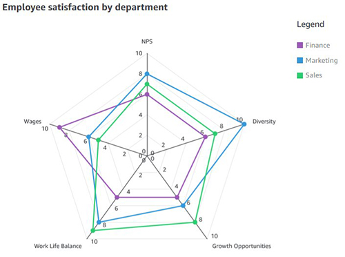
Another effective way of comparing radar charts is to compare a given department against the average or baseline value. For instance, the sales department feels less compensated compared to the baseline, but ranks high on work/life balance.

When to use radar charts
Radar charts are a great option when space is a constraint and you want to compare multiple groups in a compact space. Radar charts are best used for the following:
- Visualizing multivariate data, such as comparing cars across different stats like mileage, max speed, engine power, and driving pleasure
- Comparative analysis (comparing two or more items across a list of common variables)
- Spot outliers and commonality
Compared to parallel coordinates, radar charts are ideal when there are a few groups of items to be compared. You should also be mindful of not displaying too many variables, which can make the chart look cluttered and difficult to read.
Radar chart use cases
Radar charts have a wide variety of industry use cases, some of which are as follows:
- Sports analytics – Compare athlete performance across different performance parameters for selection criteria
- Strategy – Compare and measure different technology costs between various parameters, such as contact center, claims, massive claims, and others
- Sales – Compare performance of sales reps across different parameters like deals closed, average deal size, net new customer wins, total revenue, and deals in the pipeline
- Call centers – Compare call center staff performance against the staff average across different dimensions
- HR – Compare company scores in terms of diversity, work/life balance, benefits, and more
- User research and customer success – Compare customer satisfaction scores across different parts of the product
Different radar chart configurations
Let’s use an example of visualizing staff performance within a team, using the following sample data. The goal is to compare employee performance based on various qualities like communication, work quality, productivity, creativity, dependability, punctuality, and technical skills, ranging between a score of 0–10.
To add a radar chart to your analysis, choose the radar chart icon from the visual selector.
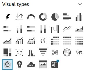
Depending on your use case and how the data is structured, you can configure radar charts in different ways.
Value as axis (UC1 and 2 tab from the dataset)
In this scenario, all qualities (communication, dependability, and so on) are defined as measures, and the employee is defined as a dimension in the dataset.

To visualize this data in a radar chart, drag all the variables to the Values field well and the Employee field to the Color field well.

Category as axis (UC1 and 2 tab from the dataset)
Another way to visualize the same data is to reverse the series and axis configuration, where each quality is displayed as a series and employees are displayed on the axis. For this, drag the Employee field to the Category field well and all the qualities to the Value field well.

Category as axis with color (UC3 tab from the dataset)
We can visualize the same use case with a different data structure, where all the qualities and employees are defined as a dimension and scores as values.
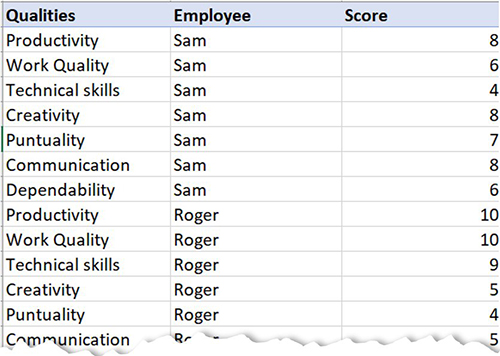
To achieve this use case, drag the field that you want to visualize as the axis to the Category field and individual series to the Color field. In our case, we chose Qualities as our axis, added Score to the Value field well, and visualized the values for each employee by adding Employee to the Color field well.

Styling radar charts
You can customize your radar charts with the following formatting options:
- Series style – You can choose to display the chart as either a line (default) or area series

- Start angle – By default, this is set to 90 degrees, but you can choose a different angle if you want to rotate the radar chart to better utilize the available real estate
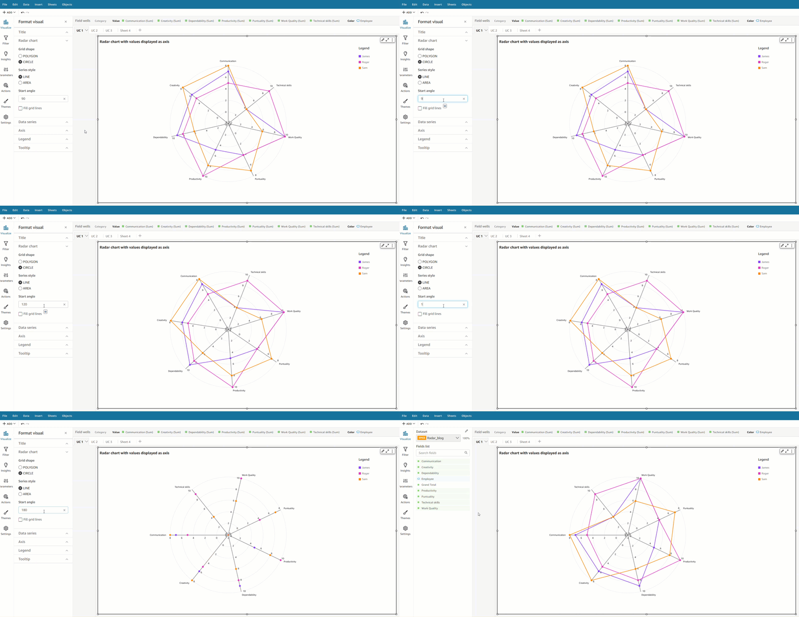
- Fill area – This option applies odd/even coloring for the plot area

- Grid shape – Choose between circle or polygon for grid shape

Summary
In this post, we looked at how radar charts can help you visualize and compare items across different variables. We also learned about the different configurations supported by radar charts and styling options to help you customize its look and feel.
We encourage you to explore radar charts and leave a comment with your feedback.
About the author
Bhupinder Chadha is a senior product manager for Amazon QuickSight focused on visualization and front end experiences. He is passionate about BI, data visualization and low-code/no-code experiences. Prior to QuickSight he was the lead product manager for Inforiver, responsible for building a enterprise BI product from ground up. Bhupinder started his career in presales, followed by a small gig in consulting and then PM for xViz, an add on visualization product.
We recently announced the general availability of Amazon OpenSearch Serverless , a new option for Amazon OpenSearch Service that makes it easy run large-scale search and analytics workloads without having to configure, manage, or scale OpenSearch clusters. With OpenSearch Serverless, you get the same interactive millisecond response times as OpenSearch Service with the simplicity of a serverless environment.
In this post, you’ll learn how to migrate your existing indices from an OpenSearch Service managed cluster domain to a serverless collection using Logstash.
With OpenSearch domains, you get dedicated, secure clusters configured and optimized for your workloads in minutes. You have full control over the configuration of compute, memory, and storage resources in clusters to optimize cost and performance for your applications. OpenSearch Serverless provides an even simpler way to run search and analytics workloads—without ever having to think about clusters. You simply create a collection and a group of indexes, and can start ingesting and querying the data.
Solution overview
Logstash is open-source software that provides ETL (extract, transform, and load) for your data. You can configure Logstash to connect to a source and a destination via input and output plugins. In between, you configure filters that can transform your data. This post walks you through the steps you need to set up Logstash to connect an OpenSearch Service domain (input) to an OpenSearch Serverless collection (output).
You set the source and destination plugins in Logstash’s config file. The config file has sections for Input, Filter, and Output. Once configured, Logstash will send a request to the OpenSearch Service domain and read the data according to the query you put in the input section. After data is read from OpenSearch Service, you can optionally send it to the next stage Filter for transformations such as adding or removing a field from the input data or updating a field with different values. In this example, you won’t use the Filter plugin. Next is the Output plugin. The open-source version of Logstash (Logstash OSS) provides a convenient way to use the bulk API to upload data to your collections. OpenSearch Serverless supports the logstash-output-opensearch output plugin, which supports AWS Identity and Access Management (IAM) credentials for data access control.
The following diagram illustrates our solution workflow.

Prerequisites
Before getting started, make sure you have completed the following prerequisites:
- Note down your OpenSearch Service domain’s ARN, user name, and password.
- Create an OpenSearch Serverless collection. If you’re new to OpenSearch Serverless, refer to Log analytics the easy way with Amazon OpenSearch Serverless for details on how to set up your collection.
Set up Logstash and the input and output plugins for OpenSearch
Complete the following steps to set up Logstash and your plugins:
- Download
logstash-oss-with-opensearch-output-plugin. (This example uses the distro for macos-x64. For other distros, refer to the artifacts.) - Extract the downloaded tarball:
- Update the
logstash-output-opensearchplugin to the latest version: - Install the
logstash-input-opensearchplugin:
Test the plugin
Let’s get into action and see how the plugin works. The following config file retrieves data from the movies index in your OpenSearch Service domain and indexes that data in your OpenSearch Serverless collection with same index name, movies.
Create a new file and add the following content, then save the file as opensearch-serverless-migration.conf. Provide the values for the OpenSearch Service domain endpoint under HOST, USERNAME, and PASSWORD in the input section, and the OpenSearch Serverless collection endpoint details under HOST along with REGION, AWS\_ACCESS\_KEY\_ID, and AWS\_SECRET\_ACCESS\_KEY in the output section.
You can specify a query in the input section of the preceding config. The match\_all query matches all data in the movies index. You can change the query if you want to select a subset of the data. You can also use the query to parallelize the data transfer by running multiple Logstash processes with configs that specify different data slices. You can also parallelize by running Logstash processes against multiple indexes if you have them.
Start Logstash
Use the following command to start Logstash:
After you run the command, Logstash will retrieve the data from the source index from your OpenSearch Service domain, and write to the destination index in your OpenSearch Serverless collection. When the data transfer is complete, Logstash shuts down. See the following code:
Verify the data in OpenSearch Serverless
You can verify that Logstash copied all your data by comparing the document count in your domain and your collection. Run the following query either from the Dev tools tab, or with curl, postman, or a similar HTTP client. The following query helps you search all documents from the movies index and returns the top documents along with the count. By default, OpenSearch will return the document count up to a maximum of 10,000. Adding the track\_total\_hits flag helps you get the exact count of documents if the document count exceeds 10,000.
Conclusion
In this post, you migrated data from your OpenSearch Service domain to your OpenSearch Serverless collection using Logstash’s OpenSearch input and output plugins.
Stay tuned for a series of posts focusing on the various options available for you to build effective log analytics and search solutions using OpenSearch Serverless. You can also refer the Getting started with Amazon OpenSearch Serverless workshop to know more about OpenSearch Serverless.
If you have feedback about this post, submit it in the comments section. If you have questions about this post, start a new thread on the Amazon OpenSearch Service forum or contact AWS Support.
About the authors
Prashant Agrawal is a Sr. Search Specialist Solutions Architect with Amazon OpenSearch Service. He works closely with customers to help them migrate their workloads to the cloud and helps existing customers fine-tune their clusters to achieve better performance and save on cost. Before joining AWS, he helped various customers use OpenSearch and Elasticsearch for their search and log analytics use cases. When not working, you can find him traveling and exploring new places. In short, he likes doing Eat → Travel → Repeat.
 Jon Handler (@\_searchgeek) is a Sr. Principal Solutions Architect at Amazon Web Services based in Palo Alto, CA. Jon works closely with the CloudSearch and Elasticsearch teams, providing help and guidance to a broad range of customers who have search workloads that they want to move to the AWS Cloud. Prior to joining AWS, Jon’s career as a software developer included four years of coding a large-scale, eCommerce search engine.
In this post, you will learn how you can use Amazon Kinesis Data Firehose to build a log ingestion pipeline to send VPC flow logs to Amazon OpenSearch Serverless. First, you create the OpenSearch Serverless collection you use to store VPC flow logs, then you create a Kinesis Data Firehose delivery pipeline that forwards the flow logs to OpenSearch Serverless. Finally, you enable delivery of VPC flow logs to your Firehose delivery stream. The following diagram illustrates the solution workflow.

OpenSearch Serverless is a new serverless option offered by Amazon OpenSearch Service. OpenSearch Serverless makes it simple to run petabyte-scale search and analytics workloads without having to configure, manage, or scale OpenSearch clusters. OpenSearch Serverless automatically provisions and scales the underlying resources to deliver fast data ingestion and query responses for even the most demanding and unpredictable workloads.
Kinesis Data Firehose is a popular service that delivers streaming data from over 20 AWS services to over 15 analytical and observability tools such as OpenSearch Serverless. Kinesis Data Firehose is great for those looking for a fast and easy way to send your VPC flow logs data to your OpenSearch Serverless collection in minutes without a single line of code and without building or managing your own data ingestion and delivery infrastructure.
VPC flow logs capture the traffic information going to and from your network interfaces in your VPC. With the launch of Kinesis Data Firehose support to OpenSearch Serverless, it makes an easy solution to analyze your VPC flow logs with just a few clicks. Kinesis Data Firehose provides a true end-to-end serverless mechanism to deliver your flow logs to OpenSearch Serverless, where you can use OpenSearch Dashboards to search through those logs, create dashboards, detect anomalies, and send alerts. VPC flow logs helps you to answer questions like:
- What percentage of your traffic is getting dropped?
- How much traffic is getting generated for specific sources and destinations?
Create your OpenSearch Serverless collection
To get started, you first create a collection. An OpenSearch Serverless collection is a logical grouping of one or more indexes that represent an analytics workload. Complete the following steps:
- On the OpenSearch Service console, choose Collections under Serverless in the navigation pane.
- Choose Create a collection.
- For Collection name, enter a name (for example,
vpc-flow-logs). - For Collection type¸ choose Time series.
- For Encryption, choose your preferred encryption setting:
- Choose Use AWS owned key to use an AWS managed key.
- Choose a different AWS KMS key to use your own AWS Key Management Service (AWS KMS) key.
- For Network access settings, choose your preferred setting:
- Choose VPC to use a VPC endpoint.
- Choose Public to use a public endpoint.
AWS recommends that you use a VPC endpoint for all production workloads. For this walkthrough, select Public.
- Choose Create.
It should take couple of minutes to create the collection.
The following graphic gives a quick demonstration of creating the OpenSearch Serverless collection via the preceding steps.

At this point, you have successfully created a collection for OpenSearch Serverless. Next, you create a delivery pipeline for Kinesis Data Firehose.
Create a Kinesis Data Firehose delivery stream
To set up a delivery stream for Kinesis Data Firehose, complete the following steps:
- On the Kinesis Data Firehose console, choose Create delivery stream.
- For Source, specify Direct PUT.
Check out Source, Destination, and Name to learn more about different sources supported by Kinesis Data Firehose.
- For Destination, choose Amazon OpenSearch Serverless.
- For Delivery stream name, enter a name (for example,
vpc-flow-logs). - Under Destination settings, in the OpenSearch Serverless collection settings, choose Browse.
- Select
vpc-flow-logs. - Choose Choose.
If your collection is still creating, wait a few minutes and try again.
- For Index, specify
vpc-flow-logs. - In the Backup settings section, select Failed data only for the Source record backup in Amazon S3.
Kinesis Data Firehose uses Amazon Simple Storage Service (Amazon S3) to back up failed data that it attempts to deliver to your chosen destination. If you want to keep all data, select All data.
- For S3 Backup Bucket, choose Browse to select an existing S3 bucket, or choose Create to create a new bucket.
- Choose Create delivery stream.
The following graphic gives a quick demonstration of creating the Kinesis Data Firehose delivery stream via the preceding steps.
At this point, you have successfully created a delivery stream for Kinesis Data Firehose, which you will use to stream data from your VPC flow logs and send it to your OpenSearch Serverless collection.

Set up the data access policy for your OpenSearch Serverless collection
Before you send any logs to OpenSearch Serverless, you need to create a data access policy within OpenSearch Serverless that allows Kinesis Data Firehose to write to the vpc-flow-logs index in your collection. Complete the following steps:
- On the Kinesis Data Firehose console, choose the Configuration tab on the details page for the vpc-flow-logs delivery stream you just created.
- In the Permissions section, note down the AWS Identity and Access Management (IAM) role.
- Navigate to the
vpc-flow-logscollection details page on the OpenSearch Serverless dashboard. - Under Data access, choose Manage data access.
- Choose Create access policy.
- In the Name and description section, specify an access policy name, add a description, and select JSON as the policy definition method.
- Add the following policy in the JSON editor. Provide the collection name and index you specified during the delivery stream creation in the policy. Provide the IAM role name that you got from the permissions page of the Firehose delivery stream, and the account ID for your AWS account.
- Choose Create.
The following graphic gives a quick demonstration of creating the data access policy via the preceding steps.

Set up VPC flow logs
In the final step of this post, you enable flow logs for your VPC with the destination as Kinesis Data Firehose, which sends the data to OpenSearch Serverless.
- Navigate to the AWS Management Console.
- Search for “VPC” and then choose Your VPCs in the search result (hover over the VPC rectangle to reveal the link).
- Choose the VPC ID link for one of your VPCs.
- On the Flow Logs tab, choose Create flow log.
- For Name, enter a name.
- Leave the Filter set to All. You can limit the traffic by selecting Accept or Reject.
- Under Destination, select Send to Kinesis Firehose in the same account.
- For Kinesis Firehose delivery stream name, choose
vpc-flow-logs. - Choose Create flow log.
The following graphic gives a quick demonstration of creating a flow log for your VPC following the preceding steps.

Examine the VPC flow logs data in your collection using OpenSearch Dashboards
You won’t be able to access your collection data until you configure data access. Data access policies allow users to access the actual data within a collection.
To create a data access policy for OpenSearch Dashboards, complete the following steps:
- Navigate to the
vpc-flow-logscollection details page on the OpenSearch Serverless dashboard. - Under Data access, choose Manage data access.
- Choose Create access policy.
- In the Name and description section, specify an access policy name, add a description, and select JSON as the policy definition method.
- Add the following policy in the JSON editor. Provide the collection name and index you specified during the delivery stream creation in the policy. Additionally, provide the IAM user and the account ID for your AWS account. You need to make sure that you have the AWS access and secret keys for the principal that you specified as an IAM user.
- Choose Create.
- Navigate to OpenSearch Serverless and choose the collection you created (
vpc-flow-logs). - Choose the OpenSearch Dashboards URL and log in with your IAM access key and secret key for the user you specified under
Principal. - Navigate to dev tools within OpenSearch Dashboards and run the following query to retrieve the VPC flow logs for your VPC:
The query returns the data as shown in the following screenshot, which contains information such as account ID, interface ID, source IP address, destination IP address, and more.

Create dashboards
After the data is flowing into OpenSearch Serverless, you can easily create dashboards to monitor the activity in your VPC. The following example dashboard shows overall traffic, accepted and rejected traffic, bytes transmitted, and some charts with the top sources and destinations.

Clean up
If you don’t want to continue using the solution, be sure to delete the resources you created:
- Return to the AWS console and in the VPCs section, disable the flow logs for your VPC.
- In the OpenSearch Serverless dashboard, delete your
vpc-flow-logscollection. - On the Kinesis Data Firehose console, delete your
vpc-flow-logsdelivery stream.
Conclusion
In this post, you created an end-to-end serverless pipeline to deliver your VPC flow logs to OpenSearch Serverless using Kinesis Data Firehose. In this example, you built a delivery pipeline for your VPC flow logs, but you can also use Kinesis Data Firehose to send logs from Amazon Kinesis Data Streams and Amazon CloudWatch, which in turn can be sent to OpenSearch Serverless collections for running analytics on those logs. With serverless solutions on AWS, you can focus on your application development rather than worrying about the ingestion pipeline and tools to visualize your logs.
Get hands-on with OpenSearch Serverless by taking the Getting Started with Amazon OpenSearch Serverless workshop and check out other pipelines for analyzing your logs.
If you have feedback about this post, share it in the comments section. If you have questions about this post, start a new thread on the Amazon OpenSearch Service forum or contact AWS Support.
About the authors
Jon Handler (@\_searchgeek) is a Principal Solutions Architect at Amazon Web Services based in Palo Alto, CA. Jon works closely with the CloudSearch and Elasticsearch teams, providing help and guidance to a broad range of customers who have search workloads that they want to move to the AWS Cloud. Prior to joining AWS, Jon’s career as a software developer included four years of coding a large-scale, eCommerce search engine.
Prashant Agrawal is a Sr. Search Specialist Solutions Architect with Amazon OpenSearch Service. He works closely with customers to help them migrate their workloads to the cloud and helps existing customers fine-tune their clusters to achieve better performance and save on cost. Before joining AWS, he helped various customers use OpenSearch and Elasticsearch for their search and log analytics use cases. When not working, you can find him traveling and exploring new places. In short, he likes doing Eat → Travel → Repeat.
In April 2022, Amazon Managed Streaming for Apache Kafka (Amazon MSK) launched an exciting new capability, Amazon MSK Serverless. Amazon MSK is a fully managed service for Apache Kafka that makes it easier for developers to build and run highly available, secure, and scalable applications based on Apache Kafka. With MSK Serverless, developers can run their applications without having to provision, configure, or optimize their Apache Kafka clusters. MSK Serverless automatically provisions and scales compute and storage resources, so developers have access to on-demand streaming capacity and storage.
Over the remainder of 2022, the team collected customer feedback and worked backward from customer requirements to add new capabilities that made MSK Serverless even better. In this post, we discuss a few of these enhancements in detail and provide an example use case.
Higher default quota for partitions in a cluster
Data in Apache Kafka is written to topics, which can be partitioned into multiple log files called partitions. When a producer application writes data to a topic, it is appended to one of these partitions. MSK Serverless launched with a maximum quota of 120 partitions per cluster. However, our customers told us that they needed more partitions per cluster for a variety of use cases, ranging from change data capture (CDC) to faster real-time data processing.
In December 2022, we increased the default quota for partitions for MSK Serverless clusters. With the increased quota, you can create up to 2,400 partitions per cluster. The 20-fold increase in the number of partitions you can have per cluster lets you create more topics per cluster and have more applications consume data in parallel. You can also implement better isolation of data with fine-grained access control. More partitions are particularly useful for CDC use cases where each table in the database has hundreds of unqiue keys, which are each mapped to a unique partition. With more partitions, you can use MSK Serverless for capturing changes in larger databases with lots of tables and hundreds of keys. Note that the 2,400 limit only applies to leader partitions. MSK Serverless creates two replicas of each partition by default at no additional cost that don’t count towards this limit.
Unlimited data retention duration
The data you produce to your topics can be retained in Apache Kafka for a configurable duration, depending on how long you need to access data using Apache Kafka consumer APIs. Typically, customers retain data for short periods of time, ranging from a few hours to a few days. Previously, MSK Serverless limited data retention to a maximum of 24 hours (1 day), which is sufficient for most popular Apache Kafka use cases. However, some use cases require customers to retain data for longer, such as retaining data for audit purposes or maintaining application recovery SLAs.
Now, with the increase in the data retention duration quota, you can retain data for as long as you need in your MSK Serverless clusters. Longer data retention is particularly useful for use cases where your consumer applications need quick access to older data. For instance, in the case of a failure, the application may need to access data from the start of the topic to reconstruct its state. Because you can now retain data in your topics for longer durations, you can restore your application’s state by accessing older data using Kafka’s consumer API, making it easier to recover from such failures. After the application recovers, you can configure your application to start consuming the data from the earliest timestamp you need to reestablish your application’s state. Note that you can only retain up to 250 GB of data per partition. As long as your partition doesn’t reach 250 GB in size, you may retain it for as long as you wish. You may create more partitions if you need more storage for a given topic.
These new quotas are available in all Regions where MSK Serverless is available. For more information, navigate to the MSK Serverless tab on the Amazon MSK pricing page and choose the Region drop-down menu.
You can also request an increase to the maximum number of partitions quota by contacting AWS Support if you need more than 2,400 partitions in a cluster. The quotas for more partitions and longer retention are applied to both existing and new clusters.
Getting started: Create a topic with 1,000 partitions and 7-day retention
In this section, we demonstrate how to create a topic in MSK Serverless, specify the number of partitions, and set its retention duration.
As a prerequisite, you must have an MSK Serverless cluster and an Apache Kafka client. Refer to Getting started using MSK Serverless clusters for step-by-step instructions.
- On your client machine, access
kafka\_2.12-2.8.1/binand run the followingexportcommand (replace the ‘my-endpoint’ with the bootstrap server string of your MSK Serverless cluster): - Run the following command to create a topic called
msk-sample-topicwith 1,000 partitions and 7-day data retention (604,800,000 milliseconds): - (Optional) Run the following command to view the details of the topic you created in step 2 above:
You will see the following result:
Clean up
To avoid incurring charges on the AWS resources created in this post, delete the MSK Serverless cluster and the Amazon Elastic Compute Cloud (Amazon EC2) instance for your client machine.
- On the Amazon MSK console, select the MSK Serverless cluster you used for this solution.
- Choose Actions, then choose Delete.
- On the Amazon EC2 console, select the instance that you created for your Apache Kafka client machine.
- Choose Instance state, then choose Terminate instance.
Conclusion
This post demonstrated how to create an MSK Serverless cluster topic with 1,000 partitions and 7-day retention. With the new quota increases, you can create up to 2,400 partitions per cluster and retain data for as long as you need. If you have comments or feedback, please feel free to leave them in the comments.
About the author
 Usama Naseem is a Senior Product Manager for Amazon MSK and focuses on MSK Serverless. Previously, he held product management roles for AWS Lambda and Amazon Fresh. He is passionate about giving customers the tools to build real-time applications in the cloud. Outside of work, he continues to be under the delusion that he will be the best squash player in the world one day.
The Amazon EMR runtime for Apache Spark is a performance-optimized runtime for Apache Spark that is 100% API compatible with open-source Apache Spark. With Amazon EMR release 6.9.0, the EMR runtime for Apache Spark supports equivalent Spark version 3.3.0.
With Amazon EMR 6.9.0, you can now run your Apache Spark 3.x applications faster and at lower cost without requiring any changes to your applications. In our performance benchmark tests, derived from TPC-DS performance tests at 3 TB scale, we found the EMR runtime for Apache Spark 3.3.0 provides a 3.5 times (using total runtime) performance improvement on average over open-source Apache Spark 3.3.0.
In this post, we analyze the results from our benchmark tests running a TPC-DS application on open-source Apache Spark and then on Amazon EMR 6.9, which comes with an optimized Spark runtime that is compatible with open-source Spark. We walk through a detailed cost analysis and finally provide step-by-step instructions to run the benchmark.
Results observed
To evaluate the performance improvements, we used an open-source Spark performance test utility that is derived from the TPC-DS performance test toolkit. We ran the tests on a seven-node (six core nodes and one primary node) c5d.9xlarge EMR cluster with the EMR runtime for Apache Spark, and a second seven-node self-managed cluster on Amazon Elastic Compute Cloud (Amazon EC2) with the equivalent open-source version of Spark. We ran both the tests with data in Amazon Simple Storage Service (Amazon S3).
Dynamic Resource Allocation (DRA) is a great feature to use for varying workloads. However, for a benchmarking exercise where we compare two platforms purely on performance, and test data volumes don’t change (3 TB in our case), we believe it’s best to avoid variability in order to run an apples-to-apples comparison. In our tests in both open-source Spark and Amazon EMR, we disabled DRA while running the benchmarking application.
The following table shows the total job runtime for all queries (in seconds) in the 3 TB query dataset between Amazon EMR version 6.9.0 and open-source Spark version 3.3.0. We observed that our TPC-DS tests had a total job runtime on Amazon EMR on Amazon EC2 that was 3.5 times faster than that using an open-source Spark cluster of the same configuration.

The per-query speedup on Amazon EMR 6.9 with and without the EMR runtime for Apache Spark is illustrated in the following chart. The horizontal axis shows each query in the 3 TB benchmark. The vertical axis shows the speedup of each query due to the EMR runtime. Notable performance gains are over 10 times faster for TPC-DS queries 24b, 72, 95, and 96.

Cost analysis
The performance improvements of the EMR runtime for Apache Spark directly translate to lower costs. We were able to realize a 67% cost savings running the benchmark application on Amazon EMR in comparison with the cost incurred to run the same application on open-source Spark on Amazon EC2 with the same cluster sizing due to reduced hours of Amazon EMR and Amazon EC2 usage. Amazon EMR pricing is for EMR applications running on EMR clusters with EC2 instances. The Amazon EMR price is added to the underlying compute and storage prices such as EC2 instance price and Amazon Elastic Block Store (Amazon EBS) cost (if attaching EBS volumes). Overall, the estimated benchmark cost in the US East (N. Virginia) Region is $27.01 per run for the open-source Spark on Amazon EC2 and $8.82 per run for Amazon EMR.
| Benchmark Job | Runtime (Hour) | Estimated Cost | Total EC2 Instance | Total vCPU | Total Memory (GiB) | Root Device (Amazon EBS) |
| Open-source Spark on Amazon EC2 (1 primary and 6 core nodes) | 2.23 | $27.01 | 7 | 252 | 504 | 20 GiB gp2 |
| Amazon EMR on Amazon EC2 (1 primary and 6 core nodes) | 0.63 | $8.82 | 7 | 252 | 504 | 20 GiB gp2 |
Cost breakdown
The following is the cost breakdown for the open-source Spark on Amazon EC2 job ($27.01):
- Total Amazon EC2 cost – (7 * $1.728 * 2.23) = (number of instances * c5d.9xlarge hourly rate * job runtime in hour) = $26.97
- Amazon EBS cost – ($0.1/730 * 20 * 7 * 2.23) = (Amazon EBS per GB-hourly rate * root EBS size * number of instances * job runtime in hour) = $0.042
The following is the cost breakdown for the Amazon EMR on Amazon EC2 job ($8.82):
- Total Amazon EMR cost – (7 * $0.27 * 0.63) = ((number of core nodes + number of primary nodes)* c5d.9xlarge Amazon EMR price * job runtime in hour) = $1.19
- Total Amazon EC2 cost – (7 * $1.728 * 0.63) = ((number of core nodes + number of primary nodes)* c5d.9xlarge instance price * job runtime in hour) = $7.62
- Amazon EBS cost – ($0.1/730 * 20 GiB * 7 * 0.63) = (Amazon EBS per GB-hourly rate * EBS size * number of instances * job runtime in hour) = $0.012
Set up OSS Spark benchmarking
In the following sections, we provide a brief outline of the steps involved in setting up the benchmarking. For detailed instructions with examples, refer to the GitHub repo.
For our OSS Spark benchmarking, we use the open-source tool Flintrock to launch our Amazon EC2-based Apache Spark cluster. Flintrock provides a quick way to launch an Apache Spark cluster on Amazon EC2 using the command line.
Prerequisites
Complete the following prerequisite steps:
- Have Python 3.7.x or above.
- Have Pip3 22.2.2 or above.
- Add the Python bin directory to your environment path. The Flintrock binary will be installed in this path.
- Run
aws configureto configure your AWS Command Line Interface (AWS CLI) shell to point to the benchmarking account. Refer to Quick configuration with aws configure for instructions. - Have a key pair with restrictive file permissions to access the OSS Spark primary node.
- Create a new S3 bucket in your test account if needed.
- Copy the TPC-DS source data as input to your S3 bucket.
- Build the benchmark application following the steps provided in Steps to build spark-benchmark-assembly application. Alternatively, you can download a pre-built spark-benchmark-assembly-3.3.0.jar if you want a Spark 3.3.0-based application.
Deploy the Spark cluster and run the benchmark job
Complete the following steps:
- Install the Flintrock tool via pip as shown in Steps to setup OSS Spark Benchmarking.
- Run the command flintrock configure, which pops up a default configuration file.
- Modify the default
config.yamlfile based on your needs. Alternatively, copy and paste the config.yaml file content to the default configure file. Then save the file to where it was. - Finally, launch the 7-node Spark cluster on Amazon EC2 via Flintrock.
This should create a Spark cluster with one primary node and six worker nodes. If you see any error messages, double-check the config file values, especially the Spark and Hadoop versions and the attributes of download-source and the AMI.
The OSS Spark cluster doesn’t come with YARN resource manager. To enable it, we need to configure the cluster.
- Download the yarn-site.xml and enable-yarn.sh files from the GitHub repo.
- Replace <private ip of primary node> with the IP address of the primary node in your Flintrock cluster.
You can retrieve the IP address from the Amazon EC2 console.
- Upload the files to all the nodes of the Spark cluster.
- Run the enable-yarn script.
- Enable Snappy support in Hadoop (the benchmark job reads Snappy compressed data).
- Download the benchmark utility application JAR file spark-benchmark-assembly-3.3.0.jar to your local machine.
- Copy this file to the cluster.
- Log in to the primary node and start YARN.
- Submit the benchmark job on the open-source Spark cluster as shown in Submit the benchmark job.
Summarize the results
Download the test result file from the output S3 bucket s3://$YOUR\_S3\_BUCKET/EC2\_TPCDS-TEST-3T-RESULT/timestamp=xxxx/summary.csv/xxx.csv. (Replace $YOUR\_S3\_BUCKET with your S3 bucket name.) You can use the Amazon S3 console and navigate to the output S3 location or use the AWS CLI.
The Spark benchmark application creates a timestamp folder and writes a summary file inside a summary.csv prefix. Your timestamp and file name will be different from the one shown in the preceding example.
The output CSV files have four columns without header names. They are:
- Query name
- Median time
- Minimum time
- Maximum time
The following screenshot shows a sample output. We have manually added column names. The way we calculate the geomean and the total job runtime is based on arithmetic means. We first take the mean of the med, min, and max values using the formula AVERAGE(B2:D2). Then we take a geometric mean of the Avg column using the formula GEOMEAN(E2:E105).

Set up Amazon EMR benchmarking
For detailed instructions, see Steps to setup EMR Benchmarking.
Prerequisites
Complete the following prerequisite steps:
- Run
aws configureto configure your AWS CLI shell to point to the benchmarking account. Refer to Quick configuration with aws configure for instructions. - Upload the benchmark application to Amazon S3.
Deploy the EMR cluster and run the benchmark job
Complete the following steps:
- Spin up Amazon EMR in your AWS CLI shell using command line as shown in Deploy EMR Cluster and run benchmark job.
- Configure Amazon EMR with one primary (c5d.9xlarge) and six core (c5d.9xlarge) nodes. Refer to create-cluster for a detailed description of AWS CLI options.
- Store the cluster ID from the response. You need this in the next step.
- Submit the benchmark job in Amazon EMR using add-steps in the AWS CLI.
Summarize the results
Summarize the results from the output bucket s3://$YOUR\_S3\_BUCKET/blog/EMRONEC2\_TPCDS-TEST-3T-RESULT in the same manner as we did for the OSS results and compare.
Clean up
To avoid incurring future charges, delete the resources you created using the instructions in the Cleanup section of the GitHub repo.
- Stop the EMR and OSS Spark clusters. You may also delete them if you don’t want to retain the content. You can delete these resources by running the script cleanup-benchmark-env.sh from a terminal in your benchmark environment.
- If you used AWS Cloud9 as your IDE for building the benchmark application JAR file using Steps to build spark-benchmark-assembly application, you may want to delete the environment as well.
Conclusion
You can run your Apache Spark workloads 3.5 times (based on total runtime) faster and at lower cost without making any changes to your applications by using Amazon EMR 6.9.0.
To keep up to date, subscribe to the Big Data Blog’s RSS feed to learn more about the EMR runtime for Apache Spark, configuration best practices, and tuning advice.
For past benchmark tests, see Run Apache Spark 3.0 workloads 1.7 times faster with Amazon EMR runtime for Apache Spark. Note that the past benchmark result of 1.7 times performance was based on geometric mean. Based on geometric mean, the performance in Amazon EMR 6.9 was two times faster.
About the authors
Sekar Srinivasan is a Sr. Specialist Solutions Architect at AWS focused on Big Data and Analytics. Sekar has over 20 years of experience working with data. He is passionate about helping customers build scalable solutions modernizing their architecture and generating insights from their data. In his spare time he likes to work on non-profit projects, especially those focused on underprivileged Children’s education.
 Prabu Ravichandran is a Senior Data Architect with Amazon Web Services, focussed on Analytics, data Lake architecture and implementation. He helps customers architect and build scalable and robust solutions using AWS services. In his free time, Prabu enjoys traveling and spending time with family.
Many customers need an ACID transaction (atomic, consistent, isolated, durable) data lake that can log change data capture (CDC) from operational data sources. There is also demand for merging real-time data into batch data. Delta Lake framework provides these two capabilities. In this post, we discuss how to handle UPSERTs (updates and inserts) of the operational data using natively integrated Delta Lake with AWS Glue, and query the Delta Lake using Amazon Athena.
We examine a hypothetical insurance organization that issues commercial policies to small- and medium-scale businesses. The insurance prices vary based on several criteria, such as where the business is located, business type, earthquake or flood coverage, and so on. This organization is planning to build a data analytical platform, and the insurance policy data is one of the inputs to this platform. Because the business is growing, hundreds and thousands of new insurance policies are being enrolled and renewed every month. Therefore, all this operational data needs to be sent to Delta Lake in near-real time so that the organization can perform various analytics, and build machine learning (ML) models to serve their customers in a more efficient and cost-effective way.
Solution overview
The data can originate from any source, but typically customers want to bring operational data to data lakes to perform data analytics. One of the solutions is to bring the relational data by using AWS Database Migration Service (AWS DMS). AWS DMS tasks can be configured to copy the full load as well as ongoing changes (CDC). The full load and CDC load can be brought into the raw and curated (Delta Lake) storage layers in the data lake. To keep it simple, in this post we opt out of the data sources and ingestion layer; the assumption is that the data is already copied to the raw bucket in the form of CSV files. An AWS Glue ETL job does the necessary transformation and copies the data to the Delta Lake layer. The Delta Lake layer ensures ACID compliance of the source data.
The following diagram illustrates the solution architecture.
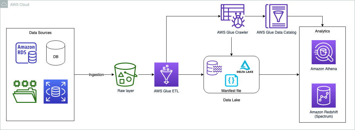
The use case we use in this post is about a commercial insurance company. We use a simple dataset that contains the following columns:
- Policy – Policy number, entered as text
- Expiry – Date that policy expires
- Location – Location type (Urban or Rural)
- State – Name of state where property is located
- Region – Geographic region where property is located
- Insured Value – Property value
- Business Type – Business use type for property, such as Farming or Retail
- Earthquake – Is earthquake coverage included (Y or N)
- Flood – Is flood coverage included (Y or N)
The dataset contains a sample of 25 insurance policies. In the case of a production dataset, it may contain millions of records.
In the following sections, we walk through the steps to perform the Delta Lake UPSERT operations. We use the AWS Management Console to perform all the steps. However, you can also automate these steps using tools like AWS CloudFormation, the AWS Cloud Development Kit (AWS CDK), Terraforms, and so on.
Prerequisites
This post is focused towards architects, engineers, developers, and data scientists who build, design, and build analytical solutions on AWS. We expect a basic understanding of the console, AWS Glue, Amazon Simple Storage Service (Amazon S3), and Athena. Additionally, the persona is able to create AWS Identity and Access Management (IAM) policies and roles, create and run AWS Glue jobs and crawlers, and is able work with the Athena query editor.
Use Athena query engine version 3 to query delta lake tables, later in the section “Query the full load using Athena”.

Set up an S3 bucket for full and CDC load data feeds
To set up your S3 bucket, complete the following steps:
- Log in to your AWS account and choose a Region nearest to you.
- On the Amazon S3 console, create a new bucket. Make sure the name is unique (for example,
delta-lake-cdc-blog-<some random number>). - Create the following folders:
- $bucket\_name/fullload – This folder is used for a one-time full load from the upstream data source
- $bucket\_name/cdcload – This folder is used for copying the upstream data changes
- $bucket\_name/delta – This folder holds the Delta Lake data files
- Copy the sample dataset and save it in a file called
full-load.csvto your local machine. - Upload the file using the Amazon S3 console into the folder
$bucket\_name/fullload.

Set up an IAM policy and role
In this section, we create an IAM policy for the S3 bucket access and a role for AWS Glue jobs to run, and also use the same role for querying the Delta Lake using Athena.
- On the IAM console, choose Polices in the navigation pane.
- Choose Create policy.
- Select JSON tab and paste the following policy code. Replace the
{bucket\_name}you created in the earlier step.
- Name the policy
delta-lake-cdc-blog-policyand select Create policy. - On the IAM console, choose Roles in the navigation pane.
- Choose Create role.
- Select AWS Glue as your trusted entity and choose Next.
- Select the policy you just created, and with two additional AWS managed policies:
delta-lake-cdc-blog-policyAWSGlueServiceRoleCloudWatchFullAccess
- Choose Next.
- Give the role a name (for example,
delta-lake-cdc-blog-role).

Set up AWS Glue jobs
In this section, we set up two AWS Glue jobs: one for full load and one for the CDC load. Let’s start with the full load job.
- On the AWS Glue console, under Data Integration and ETL in the navigation pane, choose Jobs. AWS Glue Studio opens in a new tab.
- Select Spark script editor and choose Create.

- In the script editor, replace the code with the following code snippet
- Navigate to the Job details tab.
- Provide a name for the job (for example,
Full-Load-Job). - For IAM Role¸ choose the role
delta-lake-cdc-blog-rolethat you created earlier. - For Worker type¸ choose G 2X.
- For Job bookmark, choose Disable.
- Set Number of retries to 0.
- Under Advanced properties¸ keep the default values, but provide the delta core JAR file path for Python library path and Dependent JARs path.
- Under Job parameters:
- Add the key
--s3\_bucketwith the bucket name you created earlier as the value. - Add the key
--datalake-formatsand give the valuedelta
- Add the key
- Keep the remaining default values and choose Save.

Now let’s create the CDC load job.
- Create a second job called
CDC-Load-Job. - Follow the steps on the Job details tab as with the previous job.
- Alternatively, you may choose “Clone job” option from the Full-Load-Job, this will carry all the job details from the full load job.
- In the script editor, enter the following code snippet for the CDC logic:
import sysfrom awsglue.utils import getResolvedOptionsfrom awsglue.context import GlueContextfrom pyspark.sql.session import SparkSessionfrom pyspark.sql.functions import colfrom pyspark.sql.functions import expr## For Delta lakefrom delta.tables import DeltaTable## @params: [JOB\_NAME]args = getResolvedOptions(sys.argv, ['JOB\_NAME','s3\_bucket'])# Initialize Spark Session with Delta Lakespark = SparkSession \.builder \.config("spark.sql.extensions", "io.delta.sql.DeltaSparkSessionExtension") \.config("spark.sql.catalog.spark\_catalog", "org.apache.spark.sql.delta.catalog.DeltaCatalog") \.getOrCreate()# Read the CDC loadcdc\_df = spark.read.csv("s3://"+ args['s3\_bucket']+"/cdcload")cdc\_df.show(5,True)# now read the full load (latest data) as delta tabledelta\_df = DeltaTable.forPath(spark, "s3://"+ args['s3\_bucket']+"/delta/insurance/")delta\_df.toDF().show(5,True)# UPSERT process if matches on the condition the update else insert# if there is no keyword then create a data set with Insert, Update and Delete flag and do it separately.# for delete it has to run in loop with delete condition, this script do not handle deletes. final\_df = delta\_df.alias("prev\_df").merge( \source = cdc\_df.alias("append\_df"), \#matching on primarykeycondition = expr("prev\_df.policy\_id = append\_df.\_c1"))\.whenMatchedUpdate(set= { "prev\_df.expiry\_date" : col("append\_df.\_c2"), "prev\_df.location\_name" : col("append\_df.\_c3"), "prev\_df.state\_code" : col("append\_df.\_c4"), "prev\_df.region\_name" : col("append\_df.\_c5"), "prev\_df.insured\_value" : col("append\_df.\_c6"), "prev\_df.business\_type" : col("append\_df.\_c7"), "prev\_df.earthquake\_coverage" : col("append\_df.\_c8"), "prev\_df.flood\_coverage" : col("append\_df.\_c9")} )\.whenNotMatchedInsert(values =#inserting a new row to Delta table{ "prev\_df.policy\_id" : col("append\_df.\_c1"), "prev\_df.expiry\_date" : col("append\_df.\_c2"), "prev\_df.location\_name" : col("append\_df.\_c3"), "prev\_df.state\_code" : col("append\_df.\_c4"), "prev\_df.region\_name" : col("append\_df.\_c5"), "prev\_df.insured\_value" : col("append\_df.\_c6"), "prev\_df.business\_type" : col("append\_df.\_c7"), "prev\_df.earthquake\_coverage" : col("append\_df.\_c8"), "prev\_df.flood\_coverage" : col("append\_df.\_c9")})\.execute()Run the full load job
On the AWS Glue console, open full-load-job and choose Run. The job takes about 2 minutes to complete, and the job run status changes to Succeeded. Go to $bucket\_name and open the delta folder, which contains the insurance folder. You can note the Delta Lake files in it. 
Create and run the AWS Glue crawler
In this step, we create an AWS Glue crawler with Delta Lake as the data source type. After successfully running the crawler, we inspect the data using Athena.
- On the AWS Glue console, choose Crawlers in the navigation pane.
- Choose Create crawler.
- Provide a name (for example,
delta-lake-crawler) and choose Next. - Choose Add a data source and choose Delta Lake as your data source.
- Copy your delta folder URI (for example,
s3://delta-lake-cdc-blog-123456789/delta/insurance) and enter the Delta Lake table path location. - Keep the default selection Create Native tables, and choose Add a Delta Lake data source.
- Choose Next.
- Choose the IAM role you created earlier, then choose Next.
- Select the
defaulttarget database, and providedelta\_for the table name prefix. If nodefaultdatabase exist, you may create one. - Choose Next.
- Choose Create crawler.
- Run the newly created crawler. After the crawler is complete, the
delta\_insurancetable is available underDatabases/Tables. - Open the table to check the table overview.
You can observe nine columns and their data types. 
Query the full load using Athena
In the earlier step, we created the delta\_insurance table by running a crawler against the Delta Lake location. In this section, we query the delta\_insurance table using Athena. Note that if you’re using Athena for the first time, set the query output folder to store the Athena query results (for example, s3://<your-s3-bucket>/query-output/).
- On the Athena console, open the query editor.
- Keep the default selections for Data source and Database.
- Run the query
SELECT * FROM delta\_insurance;. This query returns a total of 25 rows, the same as what was in the full load data feed. - For the CDC comparison, run the following query and store the results in a location where you can compare these results later:
The following screenshot shows the Athena query result.

Upload the CDC data feed and run the CDC job
In this section, we update three insurance policies and insert two new policies.
- Copy the following insurance policy data and save it locally as
cdc-load.csv:
The first column in the CDC feed describes the UPSERT operations. U is for updating an existing record, and I is for inserting a new record.
- Upload the cdc-load.csv file to the
$bucket\_name/cdcload/folder. - On the AWS Glue console, run
CDC-Load-Job. This job takes care of updating the Delta Lake accordingly.
The change details are as follows:
- 100462 – Expiry date changes to 12/31/2024
- 100463 – Insured value changes to 1 million
- 100475 – This policy is now under a new flood zone
- 110001 and 110002 – New policies added to the table
- Run the query again:
As shown in the following screenshot, the changes in the CDC data feed are reflected in the Athena query results.

Clean up
In this solution, we used all managed services, and there is no cost if AWS Glue jobs aren’t running. However, if you want to clean up the tasks, you can delete the two AWS Glue jobs, AWS Glue table, and S3 bucket.
Conclusion
Organizations are continuously looking at high performance, cost-effective, and scalable analytical solutions to extract the value of their operational data sources in near-real time. The analytical platform should be ready to receive changes in the operational data as soon as they occur. Typical data lake solutions face challenges to handle the changes in source data; the Delta Lake framework can close this gap. This post demonstrated how to build data lakes for UPSERT operations using AWS Glue and native Delta Lake tables, and how to query AWS Glue tables from Athena. You can implement your large scale UPSERT data operations using AWS Glue, Delta Lake and perform analytics using Amazon Athena.
References
- Introducing native Delta Lake table support with AWS Glue crawlers
- Build a high-performance, transactional data lake using open-source Delta Lake on Amazon EMR
- Build, Test and Deploy ETL solutions using AWS Glue and AWS CDK based CI/CD pipelines
- What is Delta Lake?
About the Authors
 Praveen Allam is a Solutions Architect at AWS. He helps customers design scalable, better cost-perfromant enterprise-grade applications using the AWS Cloud. He builds solutions to help organizations make data-driven decisions.
 Vivek Singh is Senior Solutions Architect with the AWS Data Lab team. He helps customers unblock their data journey on the AWS ecosystem. His interest areas are data pipeline automation, data quality and data governance, data lakes, and lake house architectures.
To build a data-driven business, it is important to democratize enterprise data assets in a data catalog. With a unified data catalog, you can quickly search datasets and figure out data schema, data format, and location. The AWS Glue Data Catalog provides a uniform repository where disparate systems can store and find metadata to keep track of data in data silos.
Apache Flink is a widely used data processing engine for scalable streaming ETL, analytics, and event-driven applications. It provides precise time and state management with fault tolerance. Flink can process bounded stream (batch) and unbounded stream (stream) with a unified API or application. After data is processed with Apache Flink, downstream applications can access the curated data with a unified data catalog. With unified metadata, both data processing and data consuming applications can access the tables using the same metadata.
This post shows you how to integrate Apache Flink in Amazon EMR with the AWS Glue Data Catalog so that you can ingest streaming data in real time and access the data in near-real time for business analysis.
Apache Flink connector and catalog architecture
Apache Flink uses a connector and catalog to interact with data and metadata. The following diagram shows the architecture of the Apache Flink connector for data read/write, and catalog for metadata read/write.
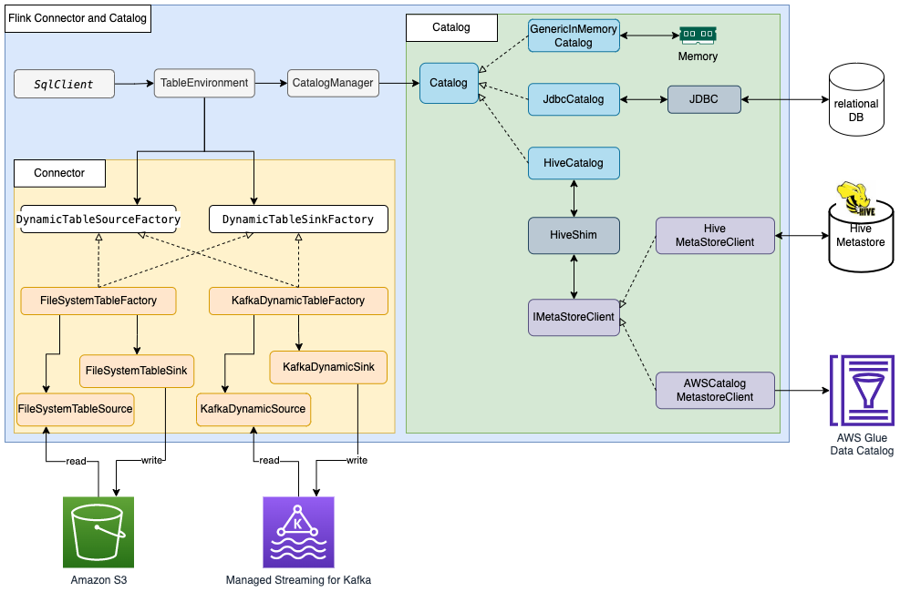
For data read/write, Flink has the interface DynamicTableSourceFactory for read and DynamicTableSinkFactory for write. A different Flink connector implements two interfaces to access data in different storage. For example, the Flink FileSystem connector has FileSystemTableFactory to read/write data in Hadoop Distributed File System (HDFS) or Amazon Simple Storage Service (Amazon S3), the Flink HBase connector has HBase2DynamicTableFactory to read/write data in HBase, and the Flink Kafka connector has KafkaDynamicTableFactory to read/write data in Kafka. You can refer to Table & SQL Connectors for more information.
For metadata read/write, Flink has the catalog interface. Flink has three built-in implementations for the catalog. GenericInMemoryCatalog stores the catalog data in memory. JdbcCatalog stores the catalog data in a JDBC-supported relational database. As of this writing, MySQL and PostgreSQL databases are supported in the JDBC catalog. HiveCatalog stores the catalog data in Hive Metastore. HiveCatalog uses HiveShim to provide different Hive version compatibility. We can configure different metastore clients to use Hive Metastore or the AWS Glue Data Catalog. In this post, we configure the Amazon EMR property hive.metastore.client.factory.class to com.amazonaws.glue.catalog.metastore.AWSGlueDataCatalogHiveClientFactory (see Using the AWS Glue Data Catalog as the metastore for Hive) so that we can use the AWS Glue Data Catalog to store Flink catalog data. Refer to Catalogs for more information.
Most Flink built-in connectors, such as for Kafka, Amazon Kinesis, Amazon DynamoDB, Elasticsearch, or FileSystem, can use Flink HiveCatalog to store metadata in the AWS Glue Data Catalog. However, some connector implementations such as Apache Iceberg have their own catalog management mechanism. FlinkCatalog in Iceberg implements the catalog interface in Flink. FlinkCatalog in Iceberg has a wrapper to its own catalog implementation. The following diagram shows the relationship between Apache Flink, the Iceberg connector, and the catalog. For more information, refer to Creating catalogs and using catalogs and Catalogs.
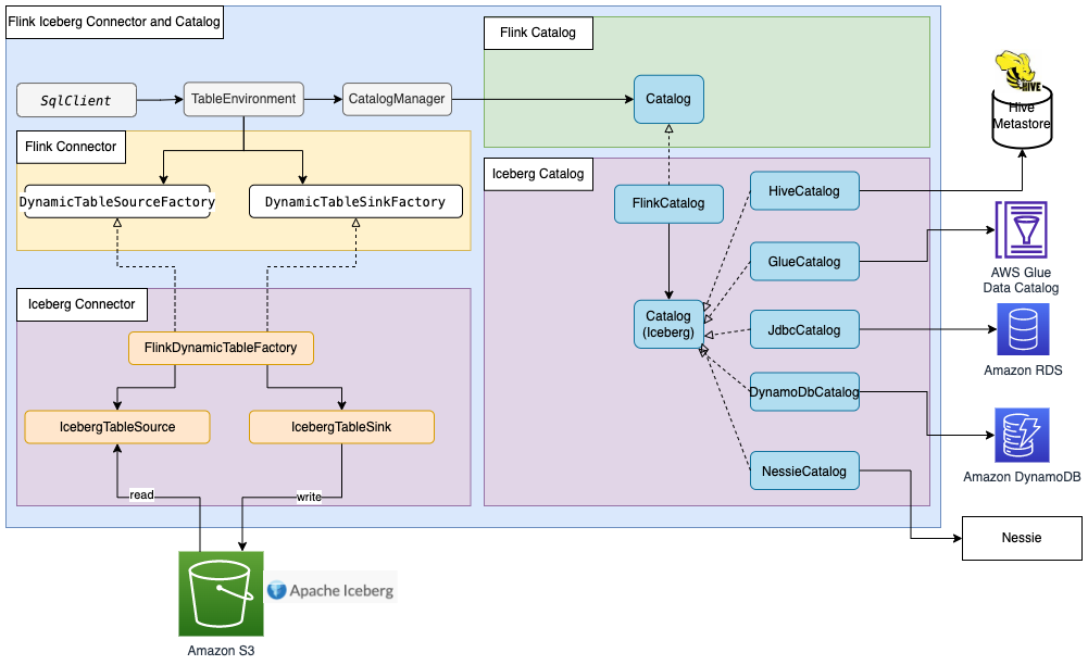
Apache Hudi also has its own catalog management. Both HoodieCatalog and HoodieHiveCatalog implements a catalog interface in Flink. HoodieCatalog stores metadata in a file system such as HDFS. HoodieHiveCatalog stores metadata in Hive Metastore or the AWS Glue Data Catalog, depending on whether you configure hive.metastore.client.factory.class to use com.amazonaws.glue.catalog.metastore.AWSGlueDataCatalogHiveClientFactory. The following diagram shows relationship between Apache Flink, the Hudi connector, and the catalog. For more information, refer to Create Catalog.

Because Iceberg and Hudi have different catalog management mechanisms, we show three scenarios of Flink integration with the AWS Glue Data Catalog in this post:
- Read/Write to Iceberg tables in Flink with metadata in Glue Data Catalog
- Read/Write to Hudi tables in Flink with metadata in Glue Data Catalog
- Read/Write to other storage format in Flink with metadata in Glue Data Catalog
Solution overview
The following diagram shows the overall architecture of the solution described in this post.
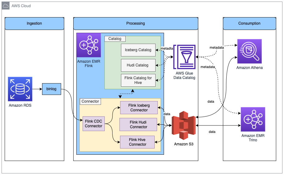
In this solution, we enable an Amazon RDS for MySQL binlog to extract transaction changes in real time. The Amazon EMR Flink CDC connector reads the binlog data and processes the data. Transformed data can be stored in Amazon S3. We use the AWS Glue Data Catalog to store the metadata such as table schema and table location. Downstream data consumer applications such as Amazon Athena or Amazon EMR Trino access the data for business analysis.
The following are the high-level steps to set up this solution:
- Enable
binlogfor Amazon RDS for MySQL and initialize the database. - Create an EMR cluster with the AWS Glue Data Catalog.
- Ingest change data capture (CDC) data with Apache Flink CDC in Amazon EMR.
- Store the processed data in Amazon S3 with metadata in the AWS Glue Data Catalog.
- Verify all table metadata is stored in the AWS Glue Data Catalog.
- Consume data with Athena or Amazon EMR Trino for business analysis.
- Update and delete source records in Amazon RDS for MySQL and validate the reflection of the data lake tables.
Prerequisites
This post uses an AWS Identity and Access Management (IAM) role with permissions for the following services:
- Amazon RDS for MySQL (5.7.40)
- Amazon EMR (6.9.0)
- Amazon Athena
- AWS Glue Data Catalog
- Amazon S3
Enable binlog for Amazon RDS for MySQL and initialize the database
To enable CDC in Amazon RDS for MySQL, we need to configure binary logging for Amazon RDS for MySQL. Refer to Configuring MySQL binary logging for more information. We also create the database salesdb in MySQL and create the tables customer, order, and others to set up the data source.
- On the Amazon RDS console, choose Parameter groups in the navigation pane.
- Create a new parameter group for MySQL.
- Edit the parameter group you just created to set
binlog\_format=ROW.
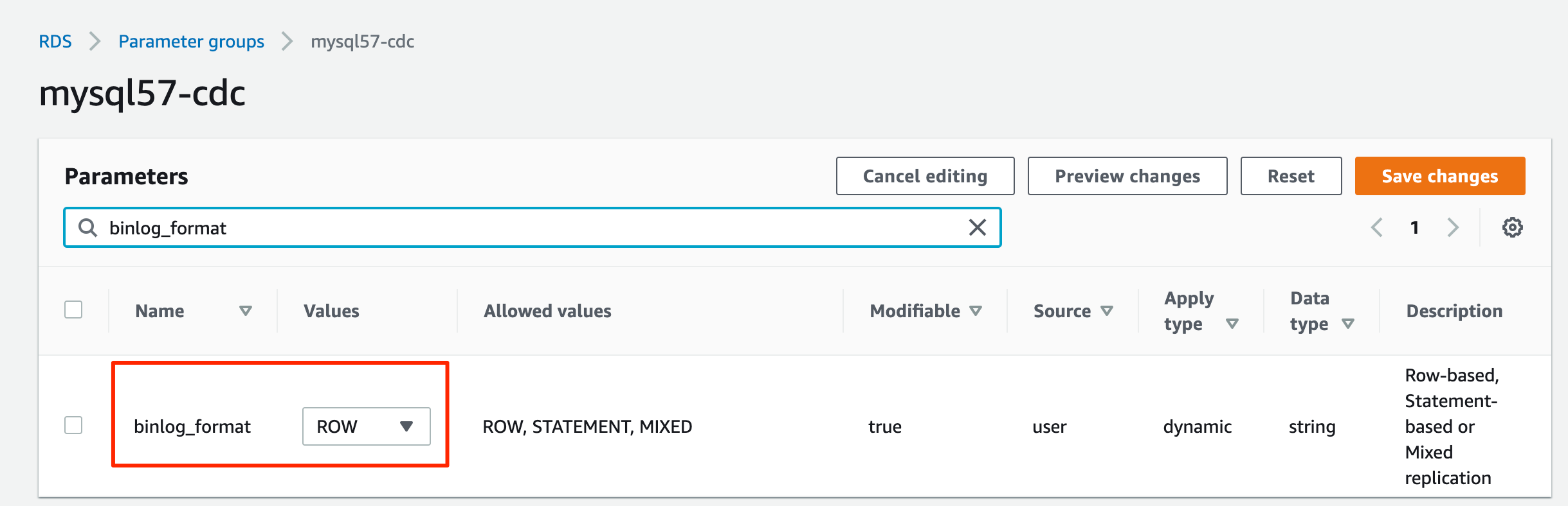
- Edit the parameter group you just created to set
binlog\_row\_image=full.
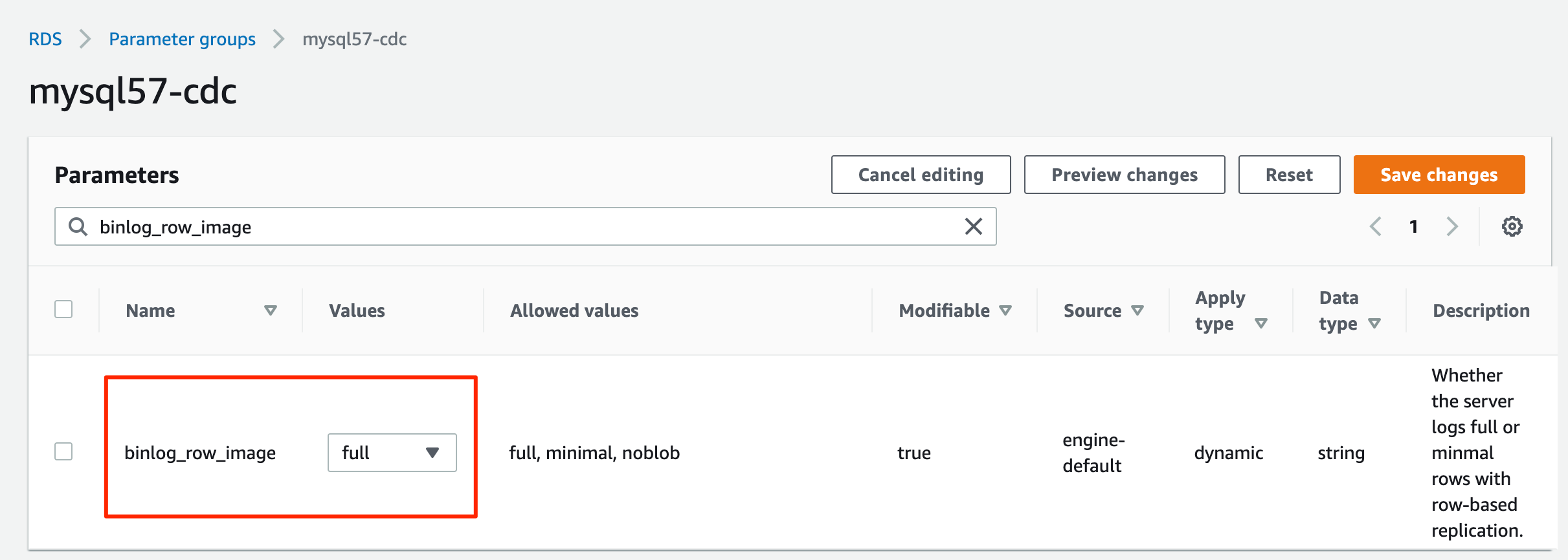
- Create an RDS for MySQL DB instance with the parameter group.
- Note down the values for
hostname,username, andpassword, which we use later. - Download the MySQL database initialization script from Amazon S3 by running the following command:
- Connect to the RDS for MySQL database and run the
salesdb.sqlcommand to initialize the database, providing the host name and user name according to your RDS for MySQL database configuration:
Create an EMR cluster with the AWS Glue Data Catalog
From Amazon EMR 6.9.0, the Flink table API/SQL can integrate with the AWS Glue Data Catalog. To use the Flink and AWS Glue integration, you must create an Amazon EMR 6.9.0 or later version.
- Create the file
iceberg.propertiesfor the Amazon EMR Trino integration with the Data Catalog. When the table format is Iceberg, your file should have following content:
- Upload
iceberg.propertiesto an S3 bucket, for exampleDOC-EXAMPLE-BUCKET.
For more information on how to integrate Amazon EMR Trino with Iceberg, refer to Use an Iceberg cluster with Trino.
- Create the file
trino-glue-catalog-setup.shto configure the Trino integration with the Data Catalog. Usetrino-glue-catalog-setup.shas the bootstrap script. Your file should have the following content (replaceDOC-EXAMPLE-BUCKETwith your S3 bucket name):
- Upload
trino-glue-catalog-setup.shto your S3 bucket (DOC-EXAMPLE-BUCKET).
Refer to Create bootstrap actions to install additional software to run a bootstrap script.
- Create the file
flink-glue-catalog-setup.shto configure the Flink integration with the Data Catalog. - Use a script runner and run the
flink-glue-catalog-setup.shscript as a step function.
Your file should have the following content (the JAR file name here is using Amazon EMR 6.9.0; a later version JAR name may change, so make sure to update according to your Amazon EMR version).
Note that here we use an Amazon EMR step, not a bootstrap, to run this script. An Amazon EMR step script is run after Amazon EMR Flink is provisioned.
- Upload
flink-glue-catalog-setup.shto your S3 bucket (DOC-EXAMPLE-BUCKET).
Refer to Configuring Flink to Hive Metastore in Amazon EMR for more information on how to configure Flink and Hive Metastore. Refer to Run commands and scripts on an Amazon EMR cluster for more details on running the Amazon EMR step script.
- Create an EMR 6.9.0 cluster with the applications Hive, Flink, and Trino.
You can create an EMR cluster with the AWS Command Line Interface (AWS CLI) or the AWS Management Console. Refer to the appropriate subsection for instructions.
Create an EMR cluster with the AWS CLI
To use the AWS CLI, complete the following steps:
- Create the file
emr-flink-trino-glue.jsonto configure Amazon EMR to use the Data Catalog. Your file should have the following content:
- Run the following command to create the EMR cluster. Provide your local
emr-flink-trino-glue.jsonparent folder path, S3 bucket, EMR cluster Region, EC2 key name, and S3 bucket for EMR logs.
Create an EMR cluster on the console
To use the console, complete the following steps:
- On the Amazon EMR console, create an EMR cluster and select Use for Hive table metadata for AWS Glue Data Catalog settings.
- Add configuration settings with the following code:

- In the Steps section, add a step called Custom JAR.
- Set JAR location to
s3://<region>.elasticmapreduce/libs/script-runner/script-runner.jar, where <region> is the region in which your EMR cluster resides. - Set Arguments to the S3 path you uploaded earlier.

- In the Bootstrap Actions section, choose Custom Action.
- Set Script location to the S3 path you uploaded.

- Continue the subsequent steps to complete your EMR cluster creation.
Ingest CDC data with Apache Flink CDC in Amazon EMR
The Flink CDC connector supports reading database snapshots and captures updates in the configured tables. We have deployed the Flink CDC connector for MySQL by downloading flink-sql-connector-mysql-cdc-2.2.1.jar and putting it into the Flink library when we create our EMR cluster. The Flink CDC connector can use the Flink Hive catalog to store Flink CDC table schema into Hive Metastore or the AWS Glue Data Catalog. In this post, we use the Data Catalog to store our Flink CDC table.
Complete the following steps to ingest RDS for MySQL databases and tables with Flink CDC and store metadata in the Data Catalog:
- SSH to the EMR primary node.
- Start Flink on a YARN session by running the following command, providing your S3 bucket name:
- Start the Flink SQL client CLI by running the following command:
- Create the Flink Hive catalog by specifying the catalog type as
hiveand providing your S3 bucket name:
Because we’re configuring the EMR Hive catalog use the AWS Glue Data Catalog, all the databases and tables created in the Flink Hive catalog are stored in the Data Catalog.
- Create the Flink CDC table, providing the host name, user name, and password for the RDS for MySQL instance you created earlier.
Note that because the RDS for MySQL user name and password will be stored in the Data Catalog as table properties, you should be enable AWS Glue database/table authorization with AWS Lake Formation to protect your sensitive data.
- Query the table you just created:
You will get a query result like following screenshot.

Store processed data in Amazon S3 with metadata in the Data Catalog
As we’re ingesting the relational database data in Amazon RDS for MySQL, raw data may be updated or deleted. To support data update and delete, we can choose data lake technologies such as Apache Iceberg or Apache Hudi to store the processed data. As we mentioned earlier, Iceberg and Hudi have different catalog management. We show both scenarios to use Flink to read/write the Iceberg and Hudi tables with metadata in the AWS Glue Data Catalog.
For non-Iceberg and non-Hudi, we use a FileSystem Parquet file to show how the Flink built-in connector uses the Data Catalog.
Read/Write to Iceberg tables in Flink with metadata in Glue Data Catalog
The following diagram shows the architecture for this configuration.

- Create a Flink Iceberg catalog using the Data Catalog by specifying
catalog-implasorg.apache.iceberg.aws.glue.GlueCatalog.
For more information about Flink and Data Catalog integration for Iceberg, refer to Glue Catalog.
- In the Flink SQL client CLI, run the following command, providing your S3 bucket name:
- Create an Iceberg table to store processed data:
- Insert the processed data into Iceberg:
Read/Write to Hudi tables in Flink with metadata in Glue Data Catalog
The following diagram shows the architecture for this configuration.
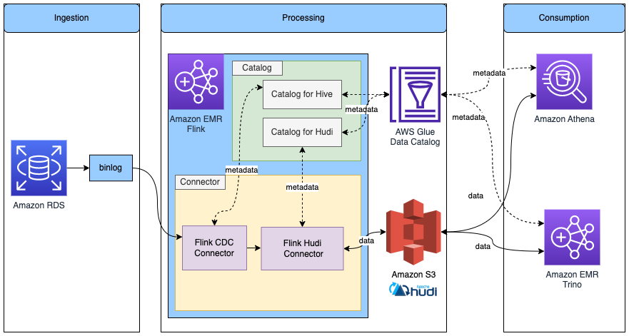
Complete the following steps:
- Create a catalog for Hudi to use the Hive catalog by specifying
modeashms.
Because we already configured Amazon EMR to use the Data Catalog when we created the EMR cluster, this Hudi Hive catalog uses the Data Catalog under the hood. For more information about Flink and Data Catalog integration for Hudi, refer to Create Catalog.
- In the Flink SQL client CLI, run the following command, providing your S3 bucket name:
- Create a Hudi table using the Data Catalog, and provide your S3 bucket name:
- Insert the processed data into Hudi:
Read/Write to other storage format in Flink with metadata in Glue Data Catalog
The following diagram shows the architecture for this configuration.
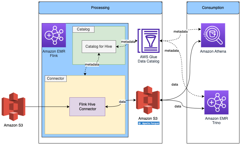
We already created the Flink Hive catalog in the previous step, so we’ll reuse that catalog.
- In the Flink SQL client CLI, run the following command:
We change the SQL dialect to Hive to create a table with Hive syntax.
- Create a table with the following SQL, and provide your S3 bucket name:
Because Parquet files don’t support updated rows, we can’t consume data from CDC data. However, we can consume data from Iceberg or Hudi.
- Use the following code to query the Iceberg table and insert data into the Parquet table:
Verify all table metadata is stored in the Data Catalog
You can navigate to the AWS Glue console to verify all the tables are stored in the Data Catalog.
- On the AWS Glue console, choose Databases in the navigation pane to list all the databases we created.

- Open a database and verify that all the tables are in that database.

Consume data with Athena or Amazon EMR Trino for business analysis
You can use Athena or Amazon EMR Trino to access the result data.
Query the data with Athena
To access the data with Athena, complete the following steps:
- Open the Athena query editor.
- Choose
flink\_glue\_iceberg\_dbfor Database.
You should see the customer\_summary table listed.
- Run the following SQL script to query the Iceberg result table:
The query result will look like the following screenshot.
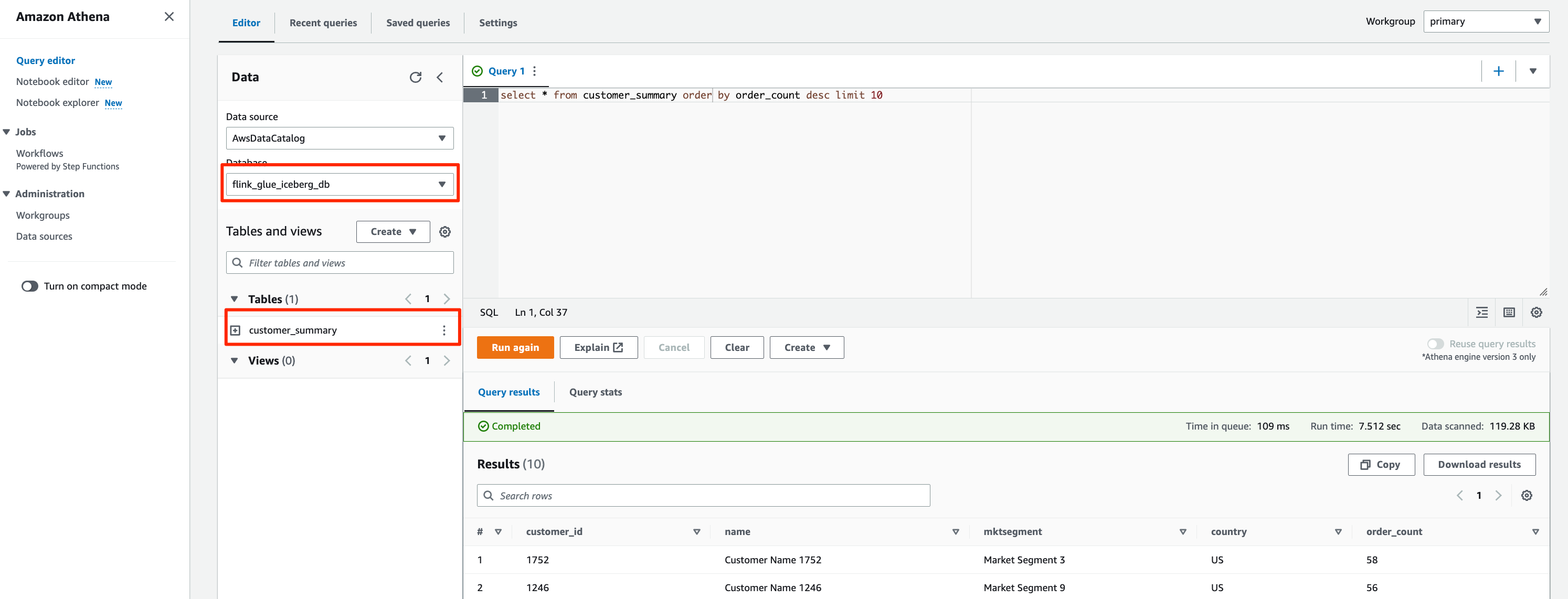
- For the Hudi table, change Database to
flink\_glue\_hudi\_dband run the same SQL query.

- For the Parquet table, change Database to
flink\_hive\_parquet\_dband run the same SQL query.

Query the data with Amazon EMR Trino
To access Iceberg with Amazon EMR Trino, SSH to the EMR primary node.
- Run the following command to start the Trino CLI:
Amazon EMR Trino can now query the tables in the AWS Glue Data Catalog.
- Run the following command to query the result table:
The query result looks like the following screenshot.

- Exit the Trino CLI.
- Start the Trino CLI with the
hivecatalog to query the Hudi table:
- Run the following command to query the Hudi table:
Update and delete source records in Amazon RDS for MySQL and validate the reflection of the data lake tables
We can update and delete some records in the RDS for MySQL database and then validate that the changes are reflected in the Iceberg and Hudi tables.
- Connect to the RDS for MySQL database and run the following SQL:
- Query the
customer\_summarytable with Athena or Amazon EMR Trino.
The updated and deleted records are reflected in the Iceberg and Hudi tables.

Clean up
When you’re done with this exercise, complete the following steps to delete your resources and stop incurring costs:
- Delete the RDS for MySQL database.
- Delete the EMR cluster.
- Drop the databases and tables created in the Data Catalog.
- Remove files in Amazon S3.
Conclusion
This post showed you how to integrate Apache Flink in Amazon EMR with the AWS Glue Data Catalog. You can use a Flink SQL connector to read/write data in a different store, such as Kafka, CDC, HBase, Amazon S3, Iceberg, or Hudi. You can also store the metadata in the Data Catalog. The Flink table API has the same connector and catalog implementation mechanism. In a single session, we can use multiple catalog instances pointing to different types, like IcebergCatalog and HiveCatalog, and use then interchangeably in your query. You can also write code with the Flink table API to develop the same solution to integrate Flink and the Data Catalog.
In our solution, we consumed the RDS for MySQL binary log directly with Flink CDC. You can also use Amazon MSK Connect to consume the binary log with MySQL Debezim and store the data in Amazon Managed Streaming for Apache Kafka (Amazon MSK). Refer to Create a low-latency source-to-data lake pipeline using Amazon MSK Connect, Apache Flink, and Apache Hudi for more information.
With the Amazon EMR Flink unified batch and streaming data processing function, you can ingest and process data with one computing engine. With Apache Iceberg and Hudi integrated in Amazon EMR, you can build an evolvable and scalable data lake. With the AWS Glue Data Catalog, you can manage all enterprise data catalogs in a unified manner and consume data easily.
Follow the steps in this post to build your unified batch and streaming solution with Amazon EMR Flink and the AWS Glue Data Catalog. Please leave a comment if you have any questions.
About the Authors
 Jianwei Li is Senior Analytics Specialist TAM. He provides consultant service for AWS enterprise support customers to design and build modern data platform.

Samrat Deb is Software Development Engineer at Amazon EMR. In his spare time, he love exploring new places, different culture and food.

Prabhu Josephraj is a Senior Software Development Engineer working for Amazon EMR. He is focused on leading the team that builds solutions in Apache Hadoop and Apache Flink. In his spare time, Prabhu enjoys spending time with his family.
Organizations with contact centers benefit from advanced analytics on their call recordings to gain important product feedback, improve contact center efficiency, and identify coaching opportunities for their staff. The Post Call Analytics (PCA) solution uses AWS machine learning (ML) services like Amazon Transcribe and Amazon Comprehend to extract insights from contact center call audio recordings uploaded after the call, or from integration with our companion Live Call Analytics (LCA) solution. You can visualize the PCA insights in the business intelligence (BI) tool Amazon QuickSight for advanced analysis.
In this post, we show you how to use PCA’s data to build automated QuickSight dashboards for advanced analytics to assist in quality assurance (QA) and quality management (QM) processes. We provide an AWS CloudFormation template and step-by-step instructions, allowing you to get started with our sample dashboard in just a few simple steps.
Sample dashboard overview
The following screenshots illustrate the different components of our sample QuickSight dashboard:
- Summary tab – This view aggregates call statistics across data points such as average customer sentiments and average agent talk duration, along with detailed call records. Graphs like “Who Talks More?” show customer sentiment distribution based on speaker talk time. You can apply data, agent, call duration, and language filters for targeted search. The graphical and tabular views help accurately analyze the data.

- Sentiment tab – This view shows sentiment distribution across multiple parameters, such as the impact of agent sentiment on customer experience. In a graphical and tabular view, you see the customer and agent sentiment score correlation. The lowest sentiment score indicates coaching opportunity for agents. You can apply data and agent filters for targeted search.

- Categories tab – This tab shows the aggregated sentiment, talk time, and non-talk time per speaker-turn in your call recordings. You can analyze the data based on category along with date and agent filter. You can get an insight into how agent speaking duration affects the customer sentiment score. The graphical and tabular views help accurately analyze the data.

- Custom Entities tab – Similar to category, you can see the breakdown across custom entities. You can apply date, agent, and custom entity filters for targeted search.

- Issues, Actions, Outcome tab – This view shows aggregated sentiment, talk time, and non-talk time per speaker-turn in your call recordings. You can analyze the data based on issue, action, and outcome for a custom phrase along with date, category, and agent filters

Solution overview
The solution uses the following AWS services and features:
- Amazon Athena
- AWS CloudFormation
- Amazon EventBridge
- AWS Glue
- AWS Identity and Access Management (IAM)
- Amazon Kinesis Data Firehose
- AWS Lambda
- Amazon QuickSight
- Amazon Simple Storage Service (Amazon S3)
The following architecture diagram shows how our solution uses PCA insights from a call recording in an S3 bucket to enable analytics in QuickSight.

As part of the solution workflow, EventBridge receives an event for each PCA solution analysis output file. Kinesis Data Firehose uses Lambda to perform data transformation and compression, storing the file in a compressed columnar format (Parquet) in the target S3 bucket. The AWS Glue Data Catalog has the table definitions for the data sources. Athena runs queries using a variety of SQL statements on the compressed Parquet files, and QuickSight is used for visualization. To optimize query performance, we use Athena partition projections. This feature automatically creates date-based partitions for query performance and cost optimization.
This is a loosely coupled architecture, with flexibility to ingest data from third-party data sources, enrich the data by adding more data points, and cross-reference data across data sources for your analytics use case. Lambda functions can integrate with third-party data sources to process and store the compressed output in Amazon S3 using Kinesis Data Firehose. Athena lets you create views by cross-referencing the data across multiple tables.
Prerequisites:
You should have the following prerequisites:
- You need an active AWS account with the permission to create and modify IAM roles
- The PCA solution must be already deployed in the same AWS account and Region that you will use for the dashboards
- QuickSight and AWS CloudFormation need to be in the same Region.
Note that this solution uses QuickSight SPICE storage.
Deploy resources with AWS CloudFormation
To deploy the solution, complete the following steps:
- Sign in to the AWS Management Console in your preferred Region.
- Create a QuickSight account (skip this step if you already have a QuickSight account):
- Navigate to the QuickSight service from the console.
- Choose Sign up for QuickSight.
- Select the edition.
- Enter your account name and notification email address.
- Navigate to the PCA solution CloudFormation stack and on the Outputs tab, note the value for the key
OutputBucket. - Allow QuickSight access to auto-discover Athena and the S3 output bucket (ref. step 3) with Write permission for Athena Workgroup enabled, then choose Finish.

- Enable EventBridge events for the PCA
OutputBucket:- Open the PCA
OutputBucket(ref. step 3) on the Amazon S3 console. - Choose Properties, scroll to Amazon EventBridge, and choose Enable
- Open the PCA
- Use the following Launch Stack button to deploy the PCA Analytics solution in your preferred Region:

- Enter a unique stack name if you want to change the default name (
pca-quicksight-analytics). - For PcaOutputBucket, enter the value of
OutputBucket. (ref. step 3) - For PcaWebAppHostAddress, enter the hostname part of the
WebAppUrloutput from your PCA stack. - Use the default values for other parameters or update if required.
- Choose Next.

- Select the acknowledgement check box and choose Create stack.
- When the CloudFormation stack creation is complete, on the QuickSight console, choose the user icon (top right) to open the menu, and choose Manage QuickSight.
- On the admin page, choose Manage assets, then choose Dashboards.
- Select
<Stack Name>-PCA-Dashboardand choose Share. - Optionally, to customize the dashboard further, share
<Stack Name>-PCA-Analysisunder Asset type analyses and<Stack Name>-PCA-*under Datasets. - Enter the QuickSight user or group and choose Share again.
Explore the dashboard with demo data
After you deploy the solution, you can explore the dashboards by loading demo data.
- Download the demo PCA files.
- Unzip and upload the demo PCA files in the
OutputBucketbucket in the/parsedFiles/folder.
Note that this step is optional. We recommend using a non-production environment or stack to keep production and demo data segregated.
Load historical PCA data
Once deployed, the solution processes new PCA data as it is added. To process older PCA data, complete the following steps:
- Open the PCA
OutputBucketon the Amazon S3 console. - Select all the content under the
/parsedFiles/folder. - Choose Action and copy the files to the same location.
This triggers an EventBridge rule to process the historical PCA files and stream the data to the QuickSight dashboard.
Validate the data
After you generate the PCA output data (within a few minutes), a compressed Parquet PCA data file will appear in the PCA OutputBucket under pca-output-base.
- On the Athena console, open the query editor and choose the
pcadatabase. You should see thepca\_outputtable under Tables and views. - Choose the options menu next to the
pca\_outputtable and choose Preview Table.

- Run your query and review the results.

Navigating the dashboard controls
- Sliders under the date-based visuals can adjust the date range.
- You can choose the segments in the visuals to drill down further. QuickSight uses the selected segment as a criterion to filter the data on the current page. To cancel this filtering, choose the same segment again.
- The bottom of each page shows grid visuals for detailed analysis.
- Similar to other visuals, you can export grid visual data to CSV and Excel from the menu at the right-top corner of the pane.
- In the grid visual, choose the ID value of each call record to go to the PCA portal to view details of this record.
- You can use filters to specify your criteria. For example, adjust
FromDateandToDateto view older data or a custom time frame.
Clean up
To remove the resources created by this stack, perform the following steps:
- Delete the CloudFormation stack.
- If you uploaded demo PCA files into your non-production PCA deployment, remove them from the PCA
OutputBucketbucket under/parsedFiles/. - Delete the
pca-output-basefolder under the PCA output bucket.
Conclusion
In this post, you learned how to visualize PCA solution data, using a CloudFormation template to automate the QuickSight dashboard creation. You also learned to how to visualize historical PCA data in QuickSight.
The sample PCA QuickSight dashboard application is provided as open source—use it as a starting point for your own solution, and help us make it better by contributing back fixes and features via GitHub pull requests. For expert assistance, AWS Professional Services and other AWS Partners are here to help.
About the Authors
 Mehmet Demir is a Senior Solutions Architect at Amazon Web Services (AWS) based in Toronto, Canada. He helps customers in building well-architected solutions that support business innovation.
 Ankur Taunk is a Senior Specialist Solutions Architect at AWS. He helps customer achieve their desired business outcomes in the Contact Center space leveraging Amazon Connect.
This post is co-written with Vidya Kotamraju and Tallis Hobbs, from Diligent.
Diligent is the global leader in modern governance, providing software as a service (SaaS) services across governance, risk, compliance, and audit, helping companies meet their environmental, social, and governance (ESG) commitments. Serving more than 1 million users from over 25,000 customers around the world, we empower transformational leaders with software, insights, and confidence to drive greater impact and lead with purpose.
We provide the right governance technology that empowers our customers to act strategically while maintaining compliance, mitigating risk, and driving efficiency. With the Diligent Platform, organizations can bring their most critical data into one centralized place. By using powerful analytics, automation, and unparalleled industry data, our customers’ board and c-suite get relevant insights from across risk, compliance, audit, and ESG teams that help them make better decisions, faster and more securely.
One of the biggest obstacles that customers face is obtaining a holistic view of their data. To effectively manage risks and ensure compliance, organizations need to have a comprehensive understanding of their operations and processes. However, this can be difficult to achieve. Scenarios such as data being dispersed across multiple systems and departments, or if data is not consistently collected and updated, or if data is not in a format that can be easily analyzed can all present various challenges. To address them, we turned to Amazon QuickSight to enhance our customer-facing products with embedded insights and reports.
In this post, we cover what we were looking for in a business intelligence (BI) tool, and how QuickSight met our requirements.
Narrowing down the competition
To effectively serve our customers, we needed a platform-wide reporting solution that would enable our users to centralize their governance, risk, and compliance (GRC) programs, and collect information from disparate data sources, while allowing for integrated automation and analytics for data-driven insights, thereby providing a curated picture of GRC with confidence.
When we started our research into various BI tool offerings to embed into our platform, we narrowed the list down to a handful that had most of the capabilities we were looking for. After reviewing the options, QuickSight was our top option when it came to the ease of integration with our existing AWS-built ecosystem. QuickSight offered everything we needed, with the flexibility we wanted, at an affordable price.
Why we chose QuickSight
There are many data points that can be useful for making business decisions; the specific data points that are most critical will depend on the nature of the business and the decisions being made. However, there are some common types of data that are often important for making informed business decisions: financial data, marketing data, operational data, and customer data.
Translating those requirements into BI tool functionality, we were looking for:
- A seamless way to obtain a holistic and unified view of data
- The ability to handle substantial amounts (over 100 TB) of data
- Enough flexibility to support the changing needs of our solution as we grow
- Great value for the price
QuickSight checked all the boxes on our list. The most compelling reasons why we ultimately chose QuickSight were:
- Visualization and reporting capabilities – QuickSight offers a wide range of visualization options and allows creation of custom reports and dashboards
- Data sources – QuickSight supports a wide variety of data sources, making connection and analysis easy
- Ease of integration – QuickSight fit seamlessly with our existing AWS technology stack with a price that fits our budget
Comprehensive, personalized, customer-facing reporting platform
Today, we’re using Quicksight to create a customer-facing reporting platform that allows our customers to report on their data within our ecosystem. QuickSight helps empower our customers by putting the reporting tools and capability in their hands, allowing them to get a comprehensive, personalized (via row-level security) view of data, unique to their workflow.
The following screenshot shows an example of our Issues & Actions dashboard, designed for risk managers and audit managers, showing various issues in need of attention.

QuickSight has provided a way to enable our customers to bring data and intelligence to the board or leadership teams in a simple, more streamlined way that saves time and effort—by automating standard reporting and surfacing it in a rich and interactive dashboard for directors. Boards and leaders will have access to curated insights, culled from both internal operations and external sources, integrated into the Diligent Boards platform—visualized in such a way that their data tells the story that accompanies the board materials.
For us, the most compelling benefit of using QuickSight is the ease of integration with Diligent’s existing tech stack and data stack. Quicksight integrates seamlessly with other AWS products in our technology stack, making it easy to incorporate data from various sources and systems into our dashboards and reports.
QuickSight was the perfect fit
Our customers love the flexibility with reporting. Quicksight provides a range of visualization options that allows users to customize their dashboards and reports to fit their specific needs and preferences. We love that the QuickSight team is open to taking prompt action on customer feedback. Their continuous and frequent feature release process is confidence-inspiring.
QuickSight helps us provide flexibility to our customers, enabling them to quickly put the right data in front of the right audience to make the right business decisions.
To learn more, visit Amazon QuickSight.
About the Authors
 Vidya Kotamraju is a Product Management Leader at Diligent, with close to 2 decades of experience leading award-winning B2B, B2C product and team success across multiple industries and geographies. Currently, she is focused on Diligent Highbond’s Data Automation Solutions.
 Tallis Hobbs is a Senior Software Engineer at Diligent. As a previous educator, he brings a unique skill set to the engineering space. He is passionate about the AWS serverless space and currently works on Diligent’s client facing Quicksight integration.
 Samit Kumbhani is a Sr. Solutions Architect at AWS based out of New York City area. Has has 18+ years of experience in building applications and focuses on Analytics, Business Intelligence and Databases. He enjoys working with customers to understand their challenges and solve them by creating innovative solutions using AWS services. Outside of work, Samit loves playing cricket, traveling and spending time with his family and friends.
AWS Glue is a serverless, scalable data integration service that makes it easier to discover, prepare, move, and integrate data from multiple sources. AWS Glue provides an extensible architecture that enables users with different data processing use cases.
A common use case is building data lakes on Amazon Simple Storage Service (Amazon S3) using AWS Glue extract, transform, and load (ETL) jobs. Data lakes free you from proprietary data formats defined by the business intelligence (BI) tools and limited capacity of proprietary storage. In addition, data lakes help you break down data silos to maximize end-to-end data insights. As data lakes have grown in size and matured in usage, a significant amount of effort can be spent keeping the data up to date by ensuring files are updated in a transactionally consistent manner.
AWS Glue customers can now use the following open-source data lake storage frameworks: Apache Hudi, Linux Foundation Delta Lake, and Apache Iceberg. These data lake frameworks help you store data and interface data with your applications and frameworks. Although popular data file formats such as Apache Parquet, CSV, and JSON can store big data, data lake frameworks bundle distributed big data files into tabular structures that are otherwise hard to manage. This makes data lake table frameworks the building constructs of databases on data lakes.
We announced general availability for native support for Apache Hudi, Linux Foundation Delta Lake, and Apache Iceberg on AWS Glue for Spark. This feature removes the need to install a separate connector or associated dependencies, manage versions, and simplifies the configuration steps required to use these frameworks in AWS Glue for Apache Spark. With these open-source data lake frameworks, you can simplify incremental data processing in data lakes built on Amazon S3 by using ACID (atomicity, consistency, isolation, durability) transactions, upserts, and deletes.
This post demonstrates how AWS Glue for Apache Spark works with Hudi, Delta, and Iceberg dataset tables, and describes typical use cases on an AWS Glue Studio notebook.
Enable Hudi, Delta, Iceberg in Glue for Apache Spark
You can use Hudi, Delta, or Iceberg by specifying a new job parameter --datalake-formats. For example, if you want to use Hudi, you need to specify the key as --datalake-formats and the value as hudi. If the option is set, AWS Glue automatically adds the required JAR files into the runtime Java classpath, and that’s all you need. You don’t need to build and configure the required libraries or install a separate connector. You can use the following library versions with this option.
| AWS Glue version | Hudi | Delta Lake | Iceberg |
| AWS Glue 3.0 | 0.10.1 | 1.0.0 | 0.13.1 |
| AWS Glue 4.0 | 0.12.1 | 2.1.0 | 1.0.0 |
If you want to use other versions of the preceding libraries, you can choose either of the following options:
- Use the connectors in AWS Marketplace. For example, you can use Iceberg 0.14.0 in AWS Glue 3.0 using the Apache Iceberg Connector for AWS Glue. Refer to Use the AWS Glue connector to read and write Apache Iceberg tables with ACID transactions and perform time travel for further details.
- Put your Hudi, Delta, or Iceberg libraries into your S3 bucket and specify the location using the –extra-jars option to include the libraries in the Java classpath. If you provide multiple JAR files, you must set them with comma-separated values. Refer to AWS Glue job parameters for more details.
If you choose either of the preceding options, you need to make sure the --datalake-formats job parameter is unspecified. For more information, see Process Apache Hudi, Delta Lake, Apache Iceberg datasets at scale, part 1: AWS Glue Studio Notebook.
Prerequisites
To continue this tutorial, you need to create the following AWS resources in advance:
- An AWS Identity and Access Management (IAM) role for your ETL job or notebook as instructed in Set up IAM permissions for AWS Glue Studio
- An S3 bucket for storing data
Process Hudi, Delta, and Iceberg datasets on an AWS Glue Studio notebook
AWS Glue Studio notebooks provide serverless notebooks with minimal setup. It makes data engineers and developers quickly and interactively explore and process their datasets. You can start using Hudi, Delta, or Iceberg in an AWS Glue Studio notebook by specifying the parameter via %%configure magic and setting the AWS Glue version to 3.0 as follows:
For more information, refer to the example notebooks available in the GitHub repository:
- Hudi SparkSQL
- Hudi DataFrame
- Delta Lake SparkSQL
- Delta Lake SparkSQL using S3 path
- Delta Lake DataFrame
- Iceberg SparkSQL
- Iceberg DataFrame
For this post, we use an Iceberg DataFrame as an example.
The following sections explain how to use an AWS Glue Studio notebook to create an Iceberg table and append records to the table.
Launch a Jupyter notebook to process Iceberg tables
Complete the following steps to launch an AWS Glue Studio notebook:
- Download the Jupyter notebook file.
- On the AWS Glue console, choose Jobs in the navigation plane.
- Under Create job, select Jupyter Notebook.

- Select Upload and edit an existing notebook.
- Upload
native\_iceberg\_dataframe.ipynbthrough Choose file under File upload.

- Choose Create.
- For Job name, enter
native\_iceberg\_dataframe. - For IAM Role, choose your IAM role.
- Choose Start notebook job.

Prepare and configure SparkSession with Iceberg configuration
Complete the following steps to configure SparkSession to process Iceberg tables:
- Run the following cell.
You can see --datalake-formats iceberg is set by the %%configure Jupyter magic command. For more information about Jupyter magics, refer to Configuring AWS Glue interactive sessions for Jupyter and AWS Glue Studio notebooks.

- Provide your S3 bucket name and bucket prefix for your Iceberg table location in the following cell, and run it.

- Run the following cells to initialize SparkSession.

- Optionally, if you previously ran the notebook, you need to run the following cell to clean up existing resources.

Now you’re ready to create Iceberg tables using the notebook.
Create an Iceberg table
Complete the following steps to create an Iceberg table using the notebook:
- Run the following cell to create a DataFrame (
df\_products) to write.
If successful, you can see the following table.

- Run the following cell to create an Iceberg table using the DataFrame.

- Now you can read data from the Iceberg table by running the following cell.

Append records to the Iceberg table
Complete the following steps to append records to the Iceberg table:
- Run the following cell to create a DataFrame (
df\_products\_appends) to append.

- Run the following cell to append the records to the table.

- Run the following cell to confirm that the preceding records are successfully appended to the table.

Clean up
To avoid incurring ongoing charges, clean up your resources:
- Run step 4 in the Prepare and configure SparkSession with Iceberg configuration section in this post to delete the table and underlying S3 objects.
- On the AWS Glue console, choose Jobs in the navigation plane.
- Select your job and on the Actions menu, choose Delete job(s).
- Choose Delete to confirm.
Considerations
With this capability, you have three different options to access Hudi, Delta, and Iceberg tables:
- Spark DataFrames, for example
spark.read.format("hudi").load("s3://path\_to\_data") - SparkSQL, for example
SELECT * FROM table - GlueContext, for example
create\_data\_frame.from\_catalog,write\_data\_frame.from\_catalog,getDataFrame, andwriteDataFrame
Learn more in Using the Hudi framework in AWS Glue, Using the Delta Lake framework in AWS Glue, and Using the Iceberg framework in AWS Glue.
Delta Lake native integration works with the catalog tables created from native Delta Lake tables by AWS Glue crawlers. This integration does not depend on manifest files. For more information, refer to Introducing native Delta Lake table support with AWS Glue crawlers.
Conclusion
This post demonstrated how to process Apache Hudi, Delta Lake, Apache Iceberg datasets using AWS Glue for Apache Spark. You can integrate your data using those data lake formats easily without struggling with library dependency management.
In subsequent posts in this series, we’ll show you how you can use AWS Glue Studio to visually author your ETL jobs with simpler configuration and setup for these data lake formats, and how to use AWS Glue workflows to orchestrate data pipelines and automate ingestion into your data lakes on Amazon S3 with AWS Glue jobs. Stay tuned!
If you have comments or feedback, please leave them in the comments.
About the authors
 Akira Ajisaka is a Senior Software Development Engineer on the AWS Glue team. He likes open-source software and distributed systems. In his spare time, he enjoys playing both arcade and console games.
Noritaka Sekiyama is a Principal Big Data Architect on the AWS Glue team. He is responsible for building software artifacts to help customers. In his spare time, he enjoys cycling with his new road bike.
 Savio Dsouza is a Software Development Manager on the AWS Glue team. His teams work on building and innovating in distributed compute systems and frameworks, namely on Apache Spark.
Amazon Kinesis Data Analytics is the easiest way to transform and analyze streaming data in real time using Apache Flink. Customers are already using Kinesis Data Analytics to perform real-time analytics on fast-moving data generated from data sources like IoT sensors, change data capture (CDC) events, gaming, social media, and many others. Apache Flink is a popular open-source framework and distributed processing engine for stateful computations over unbounded and bounded data streams.
Although building Apache Flink applications is typically the responsibility of a data engineering team, automating the deployment and provisioning infrastructure as code (IaC) is usually owned by the platform (or DevOps) team.
The following are typical responsibilities of the data engineering role:
- Write code for real-time analytics Apache Flink applications
- Roll out new application versions or roll them back (for example, in the case of a critical bug)
The following are typical responsibilities of the platform role:
- Write code for IaC
- Provision the required resources in the cloud and manage their access
In this post, we show how you can automate deployment and version updates for Kinesis Data Analytics applications and allow both Platform and engineering teams to effectively collaborate and co-own the final solution using AWS CodePipeline with the AWS Cloud Development Kit (AWS CDK).
Solution overview
To demonstrate the automated deployment and version update of a Kinesis Data Analytics application, we use the following example real-time data analytics architecture for this post.

The workflow includes the following steps:
- An AWS Lambda function (acting as data source) is the event producer pushing events on demand to Amazon Kinesis Data Streams when invoked.
- The Kinesis data stream receives and stores real-time events.
- The Kinesis Data Analytics application reads events from the data stream and performs real-time analytics on it.
Generic architecture
You can refer to the following generic architecture to adapt this example to your preferred CI/CD tool (for example, Jenkins). The overall deployment process is divided into three high-level parts:
- Infrastructure CI/CD – This portion is highlighted in orange. The infrastructure CI/CD pipeline is responsible for deploying all the real-time streaming architecture components, including the Kinesis Data Analytics application and any connected resources typically deployed using AWS CloudFormation.
- ApplicationStack – This portion is highlighted in gray. The application stack is deployed by the infrastructure CI/CD component using AWS CloudFormation.
- Application CI/CD – This portion is highlighted in green. The application CI/CD pipeline updates the Kinesis Data Analytics application in three steps:
- The pipeline builds the Java or Python source code of the Kinesis Data Analytics application and produces the application as a binary file.
- The pipeline pushes the latest binary file to the Amazon Simple Storage Service (Amazon S3) artifact bucket after a successful build as Kinesis Data Analytics application binary files are referenced from S3.
- The S3 bucket file put event triggers a Lambda function, which updates the version of the Kinesis Data Analytics application by deploying the latest binary.
The following diagram illustrates this workflow.

CI/CD architecture with CodePipeline
In this post, we implement the generic architecture using CodePipeline. The following diagram illustrates our updated architecture.
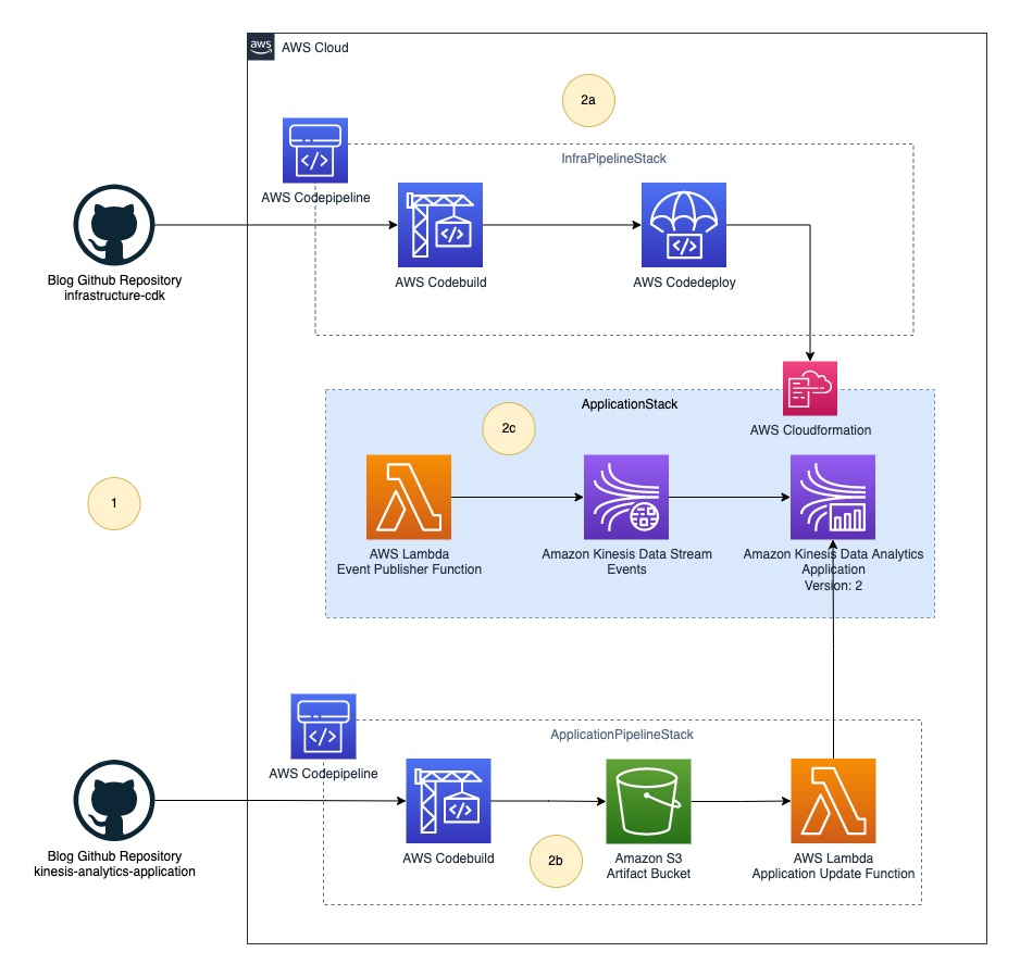
The final solution includes the following steps:
- The platform (DevOps) team and data engineering team push their source code to their respective code repositories.
- CodePipeline deploys the whole infrastructure as three stacks:
- InfraPipelineStack – Contains a pipeline to deploy the overall infrastructure.
- ApplicationPipelineStack – Contains a pipeline to build and deploy Kinesis Data Analytics application binaries. In this post, we build a Java source using the JavaBuildPipeline AWS CDK construct. You can use the PythonBuildPipeline AWS CDK construct to build a Python source.
- ApplicationStack – Contains real-time data analytics pipeline resources including Lambda (data source), Kinesis Data Streams (storage), and Kinesis Data Analytics (Apache Flink application).
Deploy resources using AWS CDK
The following GitHub repository contains the AWS CDK code to create all the necessary resources for the data pipeline. This removes opportunities for manual error, increases efficiency, and ensures consistent configurations over time. To deploy the resources, complete the following steps:
- Clone the GitHub repository to your local computer using the following command:
- Download and install the latest Node.js.
- Run the following command to install the latest version of AWS CDK:
- Run
cdk bootstrapto initialize the AWS CDK environment in your AWS account. Replace your AWS account ID and Region before running the following command.
To learn more about the bootstrapping process, refer to Bootstrapping.
Part 1: Data engineering and platform teams push source code to their code repositories
The data engineering and platform teams begin work in their respective code repositories, as illustrated in the following figure.
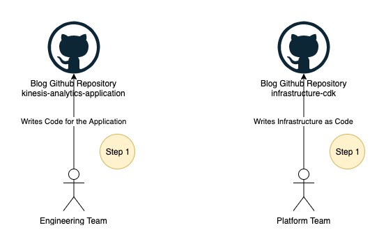
In this post, we use two folders instead of two GitHub repositories, which you can find under the root folder of the cloned repository:
- kinesis-analytics-application – This folder contains example source code of the Kinesis Data Analytics application. This represents your Kinesis Data Analytics application source code developed by your data engineering team.
- infrastructure-cdk – This folder contains example AWS CDK source code of the final solution used for provisioning all the required resources and CodePipeline. You can reuse this code for your Kinesis Data Analytics application deployment.
Application development teams usually stores the application source code in git repositories. For the demonstration purpose, we will use source code as zip file downloaded from Github instead of connecting CodePipeline to the Github repository. You may want to directly connect source repository with CodePipeline. To learn more about how to connect, refer to Create a connection to GitHub.
Part 2: The platform team deploys the application pipeline
The following figure illustrates the next step in the workflow.

In this step, you deploy the first pipeline to build the Java source code from kinesis-analytics-application. Complete the following steps to deploy ApplicationPipelineStack:
- Open your terminal, bash, or command window depending on your OS.
- Switch the current path to the folder
infrastructure-cdk. - Run
npm installto download all dependencies. - Run
cdk deploy ApplicationPipelineStackto deploy the application pipeline.
This process should take about 5 minutes to complete and deploys the following resources to your AWS account, highlighted in green in the preceding diagram:
- CodePipeline, containing stages for AWS CodeBuild and AWS CodeDeploy
- An S3 bucket to store binaries
- A Lambda function to update the Kinesis Data Analytics application JAR after manual approval
Trigger an automatic build for the application pipeline
After the cdk deploy command is successful, complete the following steps to automatically run the pipeline:
- Download the source code .zip file.
- On the AWS CloudFormation console, choose Stacks in the navigation pane.
- Choose the stack
ApplicationPipelineStack.
- On the Outputs tab, choose the link for the key
ArtifactBucketLink.
You’re redirected to the S3 artifact bucket.
- Choose Upload.
- Upload the source code .zip file you downloaded.
The first pipeline run (shown as Auto Build in the following diagram) starts automatically and takes about 5 minutes to reach the manual approval stage. The pipeline automatically downloads the source code from the artifact bucket, builds the Java project kinesis-analytics-application using Maven, and publishes the output binary JAR file back to the artifact bucket under the directory jars.

View the application pipeline run
Complete the following steps to view the application pipeline run:
- On the AWS CloudFormation console, navigate to the stack
ApplicationPipelineStack. - On the Outputs tab, choose the link for the key
ApplicationCodePipelineLink.
You’re redirected to the pipeline details page. You can see a detailed view of the pipeline, including the state of each action in each stage and the state of the transitions.
Do not approve the build for the manual approval stage yet; this is done later.
Part 3: The platform team deploys the infrastructure pipeline
The application pipeline run publishes a JAR file named kinesis-analytics-application-final.jar to the artifact bucket. Next, we deploy the Kinesis Data Analytics architecture. Complete the following steps to deploy the example flow:
- Open a terminal, bash, or command window depending on your OS.
- Switch the current path to the folder
infrastructure-cdk. - Run
cdk deploy InfraPipelineStackto deploy the infrastructure pipeline.
This process should take about 5 minutes to complete and deploys a pipeline containing stages for CodeBuild and CodeDeploy to your AWS account, as highlighted in green in the following diagram.

When the cdk deploy is complete, the infrastructure pipeline run starts automatically (shown as Auto Build 1 in the following diagram) and takes about 10 minutes to download the source code from the artifact bucket, build the AWS CDK project infrastructure-stack, and deploy ApplicationStack automatically to your AWS account. When the infrastructure pipeline run is complete, the following resources are deployed to your account (shown in green in following diagram):
- A CloudFormation template named
app-ApplicationStack - A Lambda function acting as a data source
- A Kinesis data stream acting as the stream storage
- A Kinesis Data Analytics application with the first version of
kinesis-analytics-application-final.jar
View the infrastructure pipeline run
Complete the following steps to view the application pipeline run:
- On the AWS CloudFormation console, navigate to the stack
InfraPipelineStack.
- On the Outputs tab, choose the link for the key
InfraCodePipelineLink.
You’re redirected to the pipeline details page. You can see a detailed view of the pipeline, including the state of each action in each stage and the state of the transitions.
Step 4: The data engineering team deploys the application
Now your account has everything in place for the data engineering team to work independently and roll out new versions of the Kinesis Data Analytics application. You can approve the respective application build from the application pipeline to deploy new versions of the application. The following diagram illustrates the full workflow.

The build process starts automatically when it detects changes in the source code. You can test a version update by re-uploading the source code .zip file to the S3 artifact bucket. In a real-world use case, you update the main branch either via a pull request or by merging your changes, and this action triggers a new pipeline run automatically.
View the current application version
To view the current version of the Kinesis Data Analytics application, complete the following steps:
- On the AWS CloudFormation console, navigate to the stack
InfraPipelineStack. - On the Outputs tab, choose the link for the key
KDAApplicationLink.
You’re redirected to the Kinesis Data Analytics application details page. You can find the current application version by looking at Version ID.
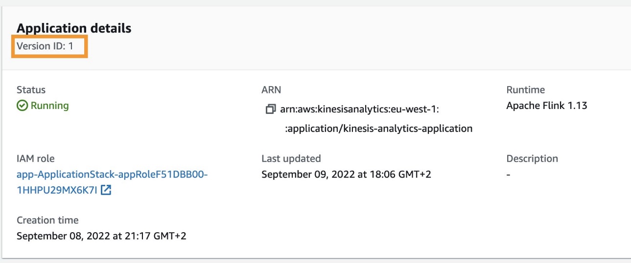
Approve the application deployment
Complete the following steps to approve the deployment (or version update) of the Kinesis Data Analytics application:
- On the AWS CloudFormation console, navigate to the stack
ApplicationPipelineStack. - On the Outputs tab, choose the link for the key
ApplicationCodePipelineLink. - Choose Review from the pipeline approval stage.

- When prompted, choose Approve to provide approval (optionally adding any comments) for the Kinesis Data Analytics application deployment or version update.

- Repeat the steps mentioned earlier to view the current application version.
You should see the application version as defined in Version ID increased by one, as shown in the following screenshot.

Deploying a new version of the Kinesis Data Analytics application will cause a downtime of around 5 minutes because the Lambda function responsible for the version update makes the API call UpdateApplication, which restarts the application after updating the version. However, the application resumes stream processing where it left off after the restart.
Clean up
Complete the following steps to delete your resources and stop incurring costs:
- On the AWS CloudFormation console, select the stack
InfraPipelineStackand choose Delete. - Select the stack
app-ApplicationStackand choose Delete. - Select stack
ApplicationPipelineStackand choose Delete. - On the Amazon S3 console, select the bucket with the name starting with
javaappCodePipelineand choose Empty. - Enter permanently delete to confirm the choice.
- Select the bucket again and choose Delete.
- Confirm the action by entering the bucket name when prompted.
- Repeat these steps to delete the bucket with the name starting with
infrapipelinestack-pipelineartifactsbucket.
Summary
This post demonstrated how to automate deployment and version updates for your Kinesis Data Analytics applications using CodePipeline and AWS CDK.
For more information, see Continuous integration and delivery (CI/CD) using CDK Pipelines and CodePipeline tutorials.
About the Author
 Anand Shah is a Big Data Prototyping Solutions Architect at AWS. He works with AWS customers and their engineering teams to build prototypes using AWS analytics services and purpose-built databases. Anand helps customers solve the most challenging problems using the art of the possible technology. He enjoys beaches in his leisure time.
Amazon QuickSight is a fast and cloud-powered business intelligence (BI) service that makes it easy to create and deliver insights to everyone in your organization without any servers or infrastructure. QuickSight dashboards can also be embedded into applications and portals to deliver insights to external stakeholders. Additionally, with Amazon QuickSight Q, end-users can simply ask questions in natural language to get machine learning (ML)-powered visual responses to their questions.
Recently, Amazon FinTech migrated all their financial reporting to QuickSight. This involved migrating complex tables and pivot tables, helping them slice and dice large datasets and deliver pixel-perfect views of their data to their stakeholders. Amazon FinTech, like all QuickSight customers, needs fast performance on very large pivot tables in order to drive adoption of their dashboards. We have specifically launched two new features focused on scaling our pivot tables with the following improvements:
- Faster loading of pivot tables during expand and collapse operations
- Increased field limits for rows, columns, and values
In this post, we discuss these improvements to pivot tables in QuickSight.
Blazing fast pivot tables during expand and collapse operations
Today, QuickSight pivot tables work as an infinite load. As users scroll vertically or horizontally on the visual, new queries are run to fetch additional rows and columns of data with fixed row and column configurations for every query request.
For example, in the following table, we would load all carrier/city combinations nested under Dec 7, 2014 before we can continue querying the next date. Let’s say we have more than 500 carrier/city rows for a specific date; this will take more than a single query to get to the next date. The count of queries run depends on the cardinality of the dimension used in the pivot table.
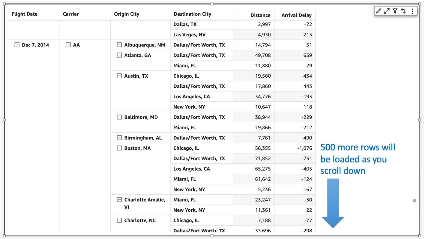
In the following example of a collapsed pivot table, since the reader doesn’t see anything beyond the flight dates, having all carrier/city rows doesn’t change what is actively displayed on the pivot table. Even though individual SQL queries can be fast, users can perceive this table to load slowly due to the sheer number of queries being fired to load the hidden (collapsed) data. Therefore, loading every single row up to the Destination City field isn’t very useful when the pivot table in the collapsed state.
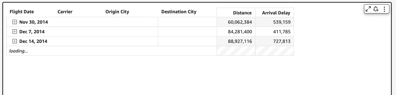
Therefore, to make our pivot tables load faster, we now only fetch the data for visible fields (expanded fields) along with a small subset of values under the collapsed field. This makes sure that data fetched in every new query is used to render new values that can be displayed immediately. We have seen customers improve their load time from 2–10 times faster depending on the complexity of their dataset.
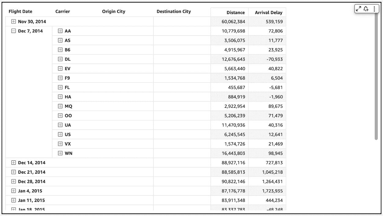
This new behavior is automatically enabled, without requiring users to do anything on their side. Please note that while we plan to support all kinds of pivot tables to use this optimization, our current rollout only includes pivot tables with only row or only column fields not sorted by any metric.
Increased field limits for pivot tables
With the ever-growing depth and granularity of data being collected, our customers asked us to increase the number of fields and data points they can display in their visuals. We have been actively listening to your needs, and just like supporting more data points in line charts, we now are increasing our field limits for pivot tables.
The value field well limits have been increased from 20 to 40, and rows and columns have been increased from 20 each to a combined limit of 40. For example, if the user has 34 fields in rows, then they can add up to 6 fields to the column field well.
This will help unblock use cases requiring increased limits such as:
- Metrics reporting – Monthly and weekly business reporting often requires having dozens of metrics presented in tabular formats. With the updated limits, you can display detailed, robust financial reports in a single pivot table rather than having to split it across multiple pivot tables.

- Migration from legacy BI and reporting tools – Existing reports in these legacy systems require displaying and slicing across a large number of row hierarchies, for example a cost center expense analysis.
- Custom use cases – These are specific industry and organization use cases where you can add dozens of values and row fields to display additional attributes. For example, a customer 360 report sliced by different regions.
As soon as you hit the limit, you receive an error message to indicate that the limit has been reached for that field well. For more details, refer to here.
 | |
Get started and stay updated!
Learn more about our new features in our newly launched QuickSight community’s Announcement section and supercharge your dashboards with the latest features from QuickSight!
About the authors
Bhupinder Chadha is a senior product manager for Amazon QuickSight focused on visualization and front end experiences. He is passionate about BI, data visualization and low-code/no-code experiences. Prior to QuickSight he was the lead product manager for Inforiver, responsible for building a enterprise BI product from ground up. Bhupinder started his career in presales, followed by a small gig in consulting and then PM for xViz, an add on visualization product.
 Igal Mizrahi is a Senior Software Engineer for AWS QuickSight Charting team. He has been part of the team for the past 3 years, and previously worked on Amazon’s mobile shopping application for 4 years.
We ended 2022 on a high note with the preview release of Amazon OpenSearch Serverless at re:Invent. Today, we are happy to announce the general availability of Amazon OpenSearch Serverless, the serverless option for Amazon OpenSearch Service that makes it easier to run search and analytics workloads without even having to think about infrastructure management. In this post, we share our approach and high-level architecture of OpenSearch Serverless.
Background
Self-managed OpenSearch and managed OpenSearch Service are widely used to search and analyze petabytes of data. Both options give you full control over the configuration of compute, memory, and storage resources in clusters, which allows you to optimize cost and performance for their applications.
However, you might often run applications that could be highly variable, where the usage is not always known. Such applications may experience sudden bursts in ingestion data or irregular and unpredictable query requests. To maintain consistent performance, you must constantly tune and resize clusters or over-provision for peak demand, which results in excess costs. Many customers wanted an even simpler experience to run search and analytics workloads that allows you to focus on your business applications without having to worry about the backend infrastructure and data management.
What does simpler mean? It means you don’t want to worry about these tasks:
- Choose and provision instances
- Manage the shard or the index size
- Index and data management for sizing and operational purposes
- Monitor or tune the settings continuously to meet workload demands
- Plan for system failures and resource threshold breaches
- Security updates and service software updates
We translated this checklist into requirements and goals under the following product themes:
- Simple and secure
- Auto scaling, fault tolerance, and durability
- Cost efficiency
- Ecosystem integrations
Before we delve into how OpenSearch Serverless addresses these needs, let’s review the target use cases for OpenSearch Serverless, as their distinctive characteristics heavily influenced our design approach and architecture.
Target use cases
The target use cases for OpenSearch Serverless are the same as OpenSearch:
- Time series analytics (also popularly known as log analytics) focuses on analyzing large volumes of semi-structured machine-generated data in real time for operational, security, and user behavior insights
- Search powers customer applications in their internal networks (application search, content management systems, legal documents) and internet-facing applications such as ecommerce website search and content search
Let’s understand the differences between the typical time series and search workloads (exceptions may vary):
- Time series workloads are write-heavy, whereas search workloads are read-heavy
- Search workloads have a smaller data corpus compared to time series
- Search workloads are more sensitive to latencies and require faster response times than time series workloads
- Queries for time series are run on recent data, whereas search queries scan the entire corpus
These characteristics heavily influenced our approach to handling and managing shards, indexes, and data for the workloads. In the next section, we review the broad themes of how OpenSearch Serverless meets customer challenges while efficiently catering to these distinctive workload traits.
Simple and secure
To get started with OpenSearch Serverless, you create a collection. Collections are a logical grouping of indexed data that works together to support a workload, while the physical resources are automatically managed in the backend. You don’t have to declare how much compute or storage is needed, or monitor the system to make sure it’s running well. To adeptly handle the two predominant workloads, OpenSearch Serverless applies different sharding and indexing strategies. Therefore, in the workflow to create a collection, you must define the collection type—time series or search. You don’t have to worry about re-indexing or rollover of indexes to support your growing data sizes, because it’s handled automatically by the system.

Next, you make the configuration choices about the encryption key to use, network access to your collections (public endpoint or VPC), and who should access your collection. OpenSearch Serverless has an easy-to-use and highly effective security model that supports hierarchical policies for your collections and indexes. You can create granular collection-level and account-level security policies for all your collections and indexes. The centralized account-level policy provides you with comprehensive visibility and control, and makes it operationally simple to secure collections at scale. For encryption policies, you can specify an AWS Key Management Service (AWS KMS) key for a single collection, all collections, or a subset of collections using a wildcard matching pattern. If rules from multiple policies match a collection, the rule closest to the fully qualified name takes precedence. You can also specify wildcard matching patterns in network and data access policies. Multiple network and data access policies can apply to a single collection, and the permissions are additive. You can update the network and data access policies for your collection at any time.
OpenSearch Dashboards can now be accessed using your SAML and AWS Identity and Access Management (IAM) credentials. OpenSearch Serverless also supports fine-grained IAM permissions so that you can define who can create, update, and delete encryption, network, and data access policies, thereby enabling organizational alignment. All the data in OpenSearch Serverless is encrypted in transit and at rest by default.

Auto scaling, fault-tolerance, and durability
OpenSearch Serverless decouples storage and compute, which allows for every layer to scale independently based on workload demands. This decoupling also allows for the isolation of indexing and query compute nodes so the fleets can run concurrently without any resource contention. The compute resources like CPU, disk utilization, memory, and hot shard state are monitored and managed by the service. When these system thresholds are breached, the service adjusts capacity so you don’t have to worry about scaling resources. For example, when an application monitoring workload receives a sudden burst of logging activities during an availability event, OpenSearch Serverless will scale out the indexing compute nodes. When these logging activities decrease and the resource consumption in the compute nodes falls below a certain threshold, OpenSearch Serverless scales the nodes back in. Similarly, when a website search engine receives a sudden spike of queries after a news event, OpenSearch Serverless automatically scales the query compute nodes to process the queries without impacting the data ingestion performance.
The following diagram illustrates this high-level architecture.
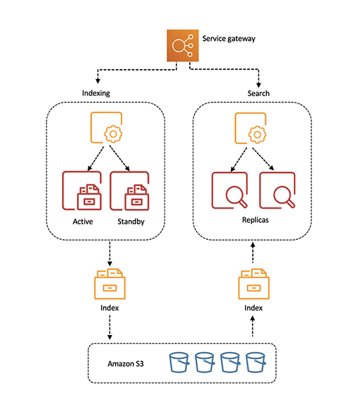
OpenSearch Serverless is designed for production workloads with redundancy for Availability Zone outages and infrastructure failures. By default, OpenSearch Serverless will replicate indexes across Availability Zones. The indexing compute nodes run in an active-standby mode. The service control plane is also built with redundancy and automatic failure recovery. All the indexed data is stored in Amazon Simple Storage Service (Amazon S3) to provide the same data durability as Amazon S3 (11 nines). The query compute instances download the indexed data directly from Amazon S3, run search operations, and perform aggregations. Redundant query compute is deployed across Availability Zones in an active-active mode to maintain availability during failures. The refresh interval (the time from when a document is ingested by OpenSearch Serverless to when it is available to search) is currently under 15 seconds.
Cost and cost efficiency
With OpenSearch Serverless, you don’t have to size or provision resources upfront, nor do you have to over-provision for peak load in production environments. You only pay for the compute and storage resources consumed by your workloads. The compute capacity used for data ingestion, and search and query is measured in OpenSearch Compute Units (OCUs). The number of OCUs corresponds directly to the CPU, memory, Amazon Elastic Block Store (Amazon EBS) storage, and the I/O resources required to ingest data or run queries. One OCU comprises 6 GB of RAM, corresponding vCPU, 120 GB of GP3 storage (used to provide fast access to the most frequently accessed data), and data transfers to Amazon S3. After data is ingested, the indexed data is stored in Amazon S3. You have the ability to control retention and delete data using the APIs.
When you create the first collection endpoint in an account, OpenSearch Serverless provisions 4 OCUs (2 ingest that include primary and standby, and 2 search that include two copies for high availability). These OCUs are instantiated even though there is no activity on the serverless endpoint to avoid any cold start latencies. All subsequent collections in that account using the same KMS key share those OCUs. During auto scaling, OpenSearch Serverless will add more OCUs to support the compute needed by your collections. These OCUs copy the indexed data from Amazon S3 before they can start responding to the indexing or query requests. Similarly, the OpenSearch Serverless control plane continuously monitors the OCUs’ resource consumption. When the indexing or search request rate decreases and the OCU consumption falls below a certain threshold, OpenSearch Serverless will reduce the OCU count to the minimum capacity required for your workload. The minimum OCUs prevent cold start delays.
OpenSearch Serverless also provides a built-in caching tier for time series workloads to provide better price-performance. OpenSearch Serverless caches the most recent log data, typically the first 24 hours, on ephemeral disk. For data older than 24 hours, OpenSearch Serverless only caches metadata and fetches the necessary data blocks from Amazon S3 based on query access. This model also helps pack more data while controlling the costs. For search collections, the query compute node caches the entire data corpus locally on ephemeral disks to provide fast, millisecond query responses.
Ecosystem integrations
Most tools that work with OpenSearch also work with OpenSearch Serverless. You don’t have to rewrite existing pipelines and applications. OpenSearch Serverless has the same logical data model and query engine of OpenSearch, so you can use the same ingest and query APIs you are familiar with, and use serverless OpenSearch Dashboards for interactive data analysis and visualization. Because of its compatible interface, OpenSearch Serverless also supports the existing rich OpenSearch ecosystem of high-level clients and streaming ingestion pipelines—Amazon Kinesis Data Firehose, FluentD, FluentBit, Logstash, Apache Kafka, and Amazon Managed Streaming for Apache Kafka (Amazon MSK). For more information, see Ingesting data into Amazon OpenSearch Serverless collections. You can also automate the process of collection creation using AWS CloudFormation and the AWS CDK. With Amazon CloudWatch integration, you can monitor key OpenSearch Serverless metrics and set alarms to notify you of any threshold breaches.
Choosing between managed clusters and OpenSearch Serverless
Both managed clusters and OpenSearch Serverless are deployment options under OpenSearch Service, and powered by the open-source OpenSearch project. OpenSearch Serverless makes it easier to run cyclical, intermittent, or unpredictable workloads without having to think about sizing, monitoring, and tuning OpenSearch clusters. You may, however, prefer to use managed clusters in scenarios where you need tight control over cluster configuration or specific customizations. With managed clusters, you can choose your preferred instances and versions, and have more control on configuration such as lower refresh intervals or data sharding strategies, which may be critical for use cases that fall outside of the typical patterns supported by OpenSearch Serverless. Also, OpenSearch Serverless currently doesn’t support all advanced OpenSearch features and plugins such as alerting, anomaly detection, and k-NN. You can use the managed clusters for these features until OpenSearch Serverless adds support for them.
Updates since the preview
With the general availability release, OpenSearch Serverless will now scale out and scale in to the minimum resources required to support your workloads. The maximum OCU limit per account has been increased from 20 to 50 for both indexing and query. Additionally, you can now use the high-level OpenSearch clients to ingest and query your data, and also migrate data from your OpenSearch clusters using Logstash. Also, we added support for three more Regions. OpenSearch Serverless is now available in eight Regions globally: US East (Ohio), US East (N. Virginia), US West (Oregon), Asia Pacific (Singapore), Asia Pacific (Sydney), Asia Pacific (Tokyo), Europe (Frankfurt), and Europe (Ireland).
Summary
The serverless journey has just begun. Most of the initial efforts were spent defining and building the right service architecture that can efficiently support the growing performance and scale demands. OpenSearch Serverless separates storage and compute components, and indexing and query compute, so they can be managed and scaled independently. OpenSearch Serverless uses Amazon S3 as the primary data storage for indexes, so you don’t need to worry about durability. We have decoupled your configuration choices from the proper provisioning of resources, so configuration mistakes won’t cause outages. OpenSearch Serverless will also apply security and software updates in the future with no disruption to your workloads. This flexible, microservices-based architecture will enable us to keep pushing out new features regularly, raising the bar on scale and performance, and driving down the costs further, for example, spinning down the compute nodes completely when there is no activity.
We encourage you to try out OpenSearch Serverless and provide your feedback in the comments section with your use cases and questions. We have a number of resources to get you started:
- AWS podcast: Introducing Amazon OpenSearch Serverless
- re:Invent 2022 video: OpenSearch Serverless, including architecture from GenPact
- Demo videos for log analytics with OpenSearch Serverless, and search applications with OpenSearch Serverless
- Getting started with Amazon OpenSearch Serverless workshop
- Amazon OpenSearch Serverless Developer Guide
About the author
 Pavani Baddepudi is a senior product manager working in search services at AWS. Her interests include distributed systems, networking, and security.
This post is co-written with Byungjun Choi and Sangha Yang from SikSin.
SikSin is a technology platform connecting customers with restaurant partners serving their multiple needs. Customers use the SikSin platform to search and discover restaurants, read and write reviews, and view photos. From the restaurateurs’ perspective, SikSin enables restaurant partners to engage and acquire customers in order to grow their business. SikSin has a partnership with 850 corporate companies and more than 50,000 restaurants. They issue restaurant e-vouchers to more than 220,000 members, including individuals as well as corporate members. The SikSin platform receives more than 3 million users in a month. SikSin was listed in the top 100 of the Financial Times’s Asia-Pacific region’s high-growth companies in 2022.
SikSin was looking to deliver improved customer experiences and increase customer engagement. SikSin confronted two business challenges:
- Customer engagement – SikSin maintains data on more than 750,000 restaurants and has more than 4,000 restaurant articles (and growing). SikSin was looking for a personalized and customized approach to provide restaurant recommendations for their customers and get them engaged with the content, thereby providing a personalized customer experience.
- Data analysis activities – The SikSin Food Service team experienced difficulties in regards to report generation due to scattered data across multiple systems. The team previously had to submit a request to the IT team and then wait for answers that might be outdated. For the IT team, they needed to manually pull data out of files, databases, and applications, and then combine them upon every request, which is a time-consuming activity. The SikSin Food Service team wanted to view web analytics log data by multiple dimensions, such as customer profiles and places. Examples include page view, conversion rate, and channels.
To overcome these two challenges, SikSin participated in the AWS Data Lab program to assist them in building a prototype solution. The AWS Data Lab offers accelerated, joint-engineering engagements between customers and AWS technical resources to create tangible deliverables that accelerate data and analytics modernization initiatives. The Build Lab is a 2–5-day intensive build with a technical customer team.
In this post, we share how SikSin built the basis for accelerating their data project with the help of the Data Lab and Amazon Personalize.
Use cases
The Data Lab team and SikSin team had three consecutive meetings to discuss business and technical requirements, and decided to work on two uses cases to resolve their two business challenges:
- Build personalized recommendations – SikSin wanted to deploy a machine learning (ML) model to produce personalized content on the landing page of the platform, particularly restaurants and restaurant articles. The success criteria was to increase the number of page views per session and membership subscription, reduce their bounce rate, and ultimately engage more visitors and members in SikSin’s contents.
- Establish self-service analytics – SikSin’s business users wanted to reduce time to insight by making data more accessible while removing the reliance on the IT team by giving business users the ability to query data. The key was to consolidate web logs from BigQuery and operational business data from Amazon Relational Data Service (Amazon RDS) into a single place and analyze data whenever they need.
Solution overview
The following architecture depicts what the SikSin team built in the 4-day Build Lab. There are two parts in the solution to address SikSin’s business and technical requirements. The first part (1–8) is for building personalized recommendations, and the second part (A–D) is for establishing self-service analytics.

SikSin deployed an ML model to produce personalized content recommendations by using the following AWS services:
- AWS Database Migration Service (AWS DMS) helps migrate databases to AWS quickly and securely with minimal downtime. The SikSin team used AWS DMS to perform full load to bring data from the database tables into Amazon Simple Storage Service (Amazon S3) as a target. Amazon S3 is an object storage service offering industry-leading scalability, data availability, security, and performance. An AWS Glue crawler populates the AWS Glue Data Catalog with the data schema definitions (in a landing folder).
- An AWS Lambda function checks if any previous files still exist in the landing folder and archives the files into a backup folder, if any.
- AWS Glue is a serverless data integration service that makes it easier to discover, prepare, move, and integrate data from multiple sources for analytics, ML, and application development. The SikSin team created AWS Glue Spark extract, transform, and load (ETL) jobs to prepare input datasets for ML models. These datasets are used to train ML models in bulk mode. There are a total of five datasets for training and two datasets for batch inference jobs.
- Amazon Personalize allows developers to quickly build and deploy curated recommendations and intelligent user segmentation at scale using ML. Because Amazon Personalize can be tailored to your individual needs, you can deliver the right customer experience at the right time and in the right place. Also, users will select existing ML models (also known as recipes), train models, and run batch inference to make recommendations.
- An Amazon Personalize job predicts for each line of input data (restaurants and restaurant articles) and produces ML-generated recommendations in the designated S3 output folder. The recommendation records are surfaced using interaction data, product data, and predictive models. An AWS Glue crawler populates the AWS Glue Data Catalog with the data schema definitions (in an output folder).
- The SikSin team applied business logics and filters in an AWS Glue job to prepare the final datasets for recommendations.
- AWS Step Functions enables you to build scalable, distributed applications using state machines. The SikSin team used AWS Step Functions Workflow Studio to visually create, run, and debug workflow runs. This workflow is triggered based on a schedule. The process includes data ingestion, cleansing, processing, and all steps defined in Amazon Personalize. This also involves managing run dependencies, scheduling, error-catching, and concurrency in accordance with the logical flow of the pipeline.
- Amazon Simple Notification Service (Amazon SNS) sends notifications. The SikSin team used Amazon SNS to send a notification via email and Google Hangouts with a Lambda function as a target.
To establish a self-service analytics environment to enable business users to perform data analysis, SikSin used the following services:
- The Google BigQuery Connector for AWS Glue simplifies the process of connecting AWS Glue jobs to extract data from BigQuery. The SikSin team used the connector to extract web analytics logs from BigQuery and load them to an S3 bucket.
- AWS Glue DataBrew is a visual data preparation tool that makes it easy for data analysts and data scientists to clean and normalize data to prepare it for analytics and ML. You can choose from over 250 pre-built transformations to automate data preparation tasks, all without the need to write any code. The SikSin Food Service team used it to visually inspect large datasets and shape the data for their data analysis activities. An S3 bucket (in the intermediate folder) contains business operational data such as customers, places, articles, and products, and reference data loaded from AWS DMS and web analytics logs and data by AWS Glue jobs.
- An AWS Glue Python shell runs a job to cleanse and join data, and apply business rules to prepare the data for queries. The SikSin team used AWS SDK Pandas, an AWS Professional Service open-source Python initiative, which extends the power of the Pandas library to AWS, connecting DataFrames and AWS data related services. The output files are stored in an Apache Parquet format in a single folder. An AWS Glue crawler populates the data schema definitions (in an output folder) into the AWS Glue Data Catalog.
- The SikSin Food Service team used Amazon Athena and Amazon Quicksight to query and visualize the data analysis. Athena is an interactive query service that makes it easy to analyze data in Amazon S3 using standard SQL. QuickSight is an ML-powered business intelligence service built for the cloud.
Business outcomes
The SikSin Food Service team is now able to access the available data for performing data analysis and manipulation operations efficiently, as well as for getting insights on their own. This immediately allows the team as well as other lines of business to understand how customers are interacting with SikSin’s contents and services on the platform and make decisions sooner. For example, with the data output, the Food Service team was able to provide insights and data points for their external stakeholder and customer to initiate a new business idea. Moreover, the team shared, “We anticipate the recommendations and personalized content will increase conversion rates and customer engagement.”
The AWS Data Lab enabled SikSin to review and assess thoroughly what data is actually usable and available. With SikSin’s objective to successfully build a data pipeline for data analytics purposes, the SikSin team came to realize the importance of data cleansing, categorization, and standardization. “Only fruitful analysis and recommendation are possible when data is intact and properly cleansed,” said Byungjun Choi (the Head of SikSin’s Food Service Team). After completing the Data Lab, SikSin completed and set up an internal process that can streamline the data cleansing pipeline.
SikSin was stuck in the research phase of looking for a solution to solve their personalization challenges. The AWS Data Lab enabled the SikSin IT Team to get hands-on with the technology and build a minimum viable product (MVP) to explore how Amazon Personalize would work in their environment with their data. They achieved this via the Data Lab by adopting AWS DMS, AWS Glue, Amazon Personalize, and Step Functions. “Though it is still the early stage of building a prototype, I am very confident with the right enablement provided from AWS that an effective recommendation system can be adopted on production level very soon,” commented Sangha Yang (the Head of SikSin IT Team).
Conclusion
As a result of the 4-day Build Lab, the SikSin team left with a working prototype that is custom fit to their needs, gaining a clear path forward for enabling end-users to gain valuable insights into its data. The Data Lab allowed the SikSin team to accelerate the architectural design and prototype build of this solution by months. Based on the lessons and learnings obtained from Data Lab, SikSin is planning to launch a Global News Content Platform equipped with a recommendation feature in FY23.
As demonstrated by SikSin’s achievements, Amazon Personalize allows developers to quickly build and deploy curated recommendations and intelligent user segmentation at scale using ML. Because Amazon Personalize can be tailored to your individual needs, you can deliver the right customer experience at the right time and in the right place. Whether you want to optimize recommendations, target customers more accurately, maximize your data’s value, or promote items using business rules.
To accelerate your digital transformation with ML, the Data Lab program is available to support you by providing prescriptive architectural guidance on a particular use case, sharing best practices, and removing technical roadblocks. You’ll leave the engagement with an architecture or working prototype that is custom fit to your needs, a path to production, and deeper knowledge of AWS services.
Please contact your AWS Account Manager or Solutions Architect to get started. If you don’t have an AWS Account Manager, please contact Sales.
About the Authors
 Byungjun Choi is the Head of SikSin Food Service at SikSin.
 Sangha Yang is the Head of IT team at SinSin.
Younggu Yun is a Senior Data Lab Architect at AWS. He works with customers around the APAC region to help them achieve business goals and solve technical problems by providing prescriptive architectural guidance, sharing best practices, and building innovative solutions together.
 Junwoo Lee is an Account Manager at AWS. He provides technical and business support to help customer resolve their problems and enrich customer journey by introducing local and global programs for his customers.
 Jinwoo Park is a Senior Solutions Architect at AWS. He provides technical support for AWS customers to succeed with their cloud journey. He helps customers build more secure, efficient, and cost-optimized architectures and solutions, and delivers best practices and workshops.
AWS Lake Formation helps with enterprise data governance and is important for a data mesh architecture. It works with the AWS Glue Data Catalog to enforce data access and governance. Both services provide reliable data storage, but some customers want replicated storage, catalog, and permissions for compliance purposes.
This post explains how to create a design that automatically backs up Amazon Simple Storage Service (Amazon S3), the AWS Glue Data Catalog, and Lake Formation permissions in different Regions and provides backup and restore options for disaster recovery. These mechanisms can be customized for your organization’s processes. The utility for cloning and experimentation is available in the open-sourced GitHub repository.
This solution only replicates metadata in the Data Catalog, not the actual underlying data. To have a redundant data lake using Lake Formation and AWS Glue in an additional Region, we recommend replicating the Amazon S3-based storage using S3 replication, S3 sync, aws-s3-copy-sync-using-batch or S3 Batch replication process. This ensures that the data lake will still be functional in another Region if Lake Formation has an availability issue. The Data Catalog setup (tables, databases, resource links) and Lake Formation setup (permissions, settings) must also be replicated in the backup Region.
Solution overview
This post shows how to create a backup of the Lake Formation permissions and AWS Glue Data Catalog from one Region to another in the same account. The solution doesn’t create or modify AWS Identity and Access Management (IAM) roles, which are available in all Regions. There are three steps to creating a multi-Region data lake:
- Migrate Lake Formation data permissions.
- Migrate AWS Glue databases and tables.
- Migrate Amazon S3 data.

In the following sections, we look at each migration step in more detail.
Lake Formation permissions
In Lake Formation, there are two types of permissions: metadata access and data access.
Metadata access permissions allow users to create, read, update, and delete metadata databases and tables in the Data Catalog.
Data access permissions allow users to read and write data to specific locations in Amazon S3. Data access permissions are managed using data location permissions, which allow users to create and alter metadata databases and tables that point to specific Amazon S3 locations.
When data is migrated from one Region to another, only the metadata access permissions are replicated. This means that if data is moved from a bucket in the source Region to another bucket in the target Region, the data access permissions need to be reapplied in the target Region.
AWS Glue Data Catalog
The AWS Glue Data Catalog is a central repository of metadata about data stored in your data lake. It contains references to data that is used as sources and targets in AWS Glue ETL (extract, transform, and load) jobs, and stores information about the location, schema, and runtime metrics of your data. The Data Catalog organizes this information in the form of metadata tables and databases. A table in the Data Catalog is a metadata definition that represents the data in a data lake, and databases are used to organize these metadata tables.
Lake Formation permissions can only be applied to objects that already exist in the Data Catalog in the target Region. Therefore, in order to apply these permissions, the underlying Data Catalog databases and tables must already exist in the target Region. To meet this requirement, this utility migrates both the AWS Glue databases and tables from the source Region to the target Region.
Amazon S3 data
The data that underlies an AWS Glue table can be stored in an S3 bucket in any Region, so replication of the data itself isn’t necessary. However, if the data has already been replicated to the target Region, this utility has the option to update the table’s location to point to the replicated data in the target Region. If the location of the data is changed, the utility updates the S3 bucket name and keeps the rest of the prefix hierarchy unchanged.
This utility doesn’t include the migration of data from the source Region to the target Region. Data migration must be performed separately using methods such as S3 replication, S3 sync, aws-s3-copy-sync-using-batch or S3 Batch replication.
This utility has two modes for replicating Lake Formation and Data Catalog metadata: on-demand and real-time. The on-demand mode is a batch replication that takes a snapshot of the metadata at a specific point in time and uses it to synchronize the metadata. The real-time mode replicates changes made to the Lake Formation permissions or Data Catalog in near-real time.
The on-demand mode of this utility is recommended for creating existing Lake Formation permissions and Data Catalogs because it replicates a snapshot of the metadata. After the Lake Formation and Data Catalogs are synchronized, you can use real-time mode to replicate any ongoing changes. This creates a mirror image of the source Region in the target Region and keeps it up to date as changes are made in the source Region. These two modes can be used independently of each other, and the operations are idempotent.
The code for the on-demand and real-time modes is available in the GitHub repository. Let’s look at each mode in more detail.
On-demand mode
On-demand mode is used to copy the Lake Formation permissions and Data Catalog at a specific point in time. The code is deployed using the AWS Cloud Development Kit (AWS CDK). The following diagram shows the solution architecture for this mode.

The AWS CDK deploys an AWS Glue job to perform the replication. The job retrieves configuration information from a file stored in an S3 bucket. This file includes details such as the source and target Regions, an optional list of databases to replicate, and options for moving data to a different S3 bucket. More information about these options and deployment instructions is available in the GitHub repository.
The AWS Glue job retrieves the Lake Formation permissions and Data Catalog object metadata from the source Region and stores it in a JSON file in an S3 bucket. The same job then uses this file to create the Lake Formation permissions and Data Catalog databases and tables in the target Region.
This tool can be run on demand by running the AWS Glue job. It copies the Lake Formation permissions and Data Catalog object metadata from the source Region to the target Region. If you run the tool again after making changes to the target Region, the changes are replaced with the latest Lake Formation permissions and Data Catalog from the source Region.
This utility can detect any changes made to the Data Catalog metadata, databases, tables, and columns while replicating the Data Catalog from the source to the target Region. If a change is detected in the source Region, the latest version of the AWS Glue object is applied to the target Region. The utility reports the number of objects modified during its run.
The Lake Formation permissions are copied from the source to the target Region, so any new permissions are replicated in the target Region. If a permission is removed from the source Region, it is not removed from the target Region.
Real-time mode
Real-time mode replicates the Lake Formation permissions and Data Catalog at a regular interval. The default interval is 1 minute, but it can be modified during deployment. The code is deployed using the AWS CDK. The following diagram shows the solution architecture for this mode.

The AWS CDK deploys two AWS Lambda jobs and creates an Amazon DynamoDB table to store AWS CloudTrail events and an Amazon EventBridge rule to run the replication at a regular interval. The Lambda jobs retrieve the configuration information from a file stored in an S3 bucket. This file includes details such as the source and target Regions, options for moving data to a different S3 bucket, and the lookback period for CloudTrail in hours. More information about these options and deployment instructions is available in the GitHub repository.
The EventBridge rule triggers a Lambda job at a fixed interval. This job retrieves the configuration information and queries CloudTrail events related to the Data Catalog and Lake Formation that occurred in the past hour (the duration is configurable). All relevant events are then stored in a DynamoDB table.
After the event information is inserted into the DynamoDB table, another Lambda job is triggered. This job retrieves the configuration information and queries the DynamoDB table. It then applies all the changes to the target Region. If the tool is run again after making changes to the target Region, the changes are replaced with the latest Lake Formation permissions and Data Catalog from the source Region. Unlike on-demand mode, this utility also removes any Lake Formation permissions that were removed from the source Region from the target Region.
Limitations
This utility is designed to replicate permissions within a single account only. The on-demand mode replicates a snapshot and doesn’t remove existing permissions, so it doesn’t perform delete operations. The API currently doesn’t support replicating changes to row and column permissions.
Conclusion
In this post, we showed how you can use this utility to migrate the AWS Glue Data Catalog and Lake Formation permissions from one Region to another. It can also keep the source and target Regions synchronized if any changes are made to the Data Catalog or the Lake Formation permissions. Implementing it across Regions (multi-Region) is a good option if you are looking for the most separation and complete independence of your globally diverse data workloads. Also consider the trade-offs. Implementing and operating this strategy, particularly using multi-Region, can be more complicated and more expensive, than other DR strategies.
To get started, checkout the github repo. For more resources, refer to the following:
About the authors
 Vivek Shrivastava is a Principal Data Architect, Data Lake in AWS Professional Services. He is a Bigdata enthusiast and holds 13 AWS Certifications. He is passionate about helping customers build scalable and high-performance data analytics solutions in the cloud. In his spare time, he loves reading and finds areas for home automation
 Raza Hafeez is a Senior Data Architect within the Shared Delivery Practice of AWS Professional Services. He has over 12 years of professional experience building and optimizing enterprise data warehouses and is passionate about enabling customers to realize the power of their data. He specializes in migrating enterprise data warehouses to AWS Modern Data Architecture.
 Nivas Shankar is a Principal Product Manager for AWS Lake Formation. He works with customers around the globe to translate business and technical requirements into products that enable customers to improve how they manage, secure and access data lake. Also leads several data and analytics initiatives within AWS including support for Data Mesh.
Serverless applications are a modernized way to perform analytics among business departments and engineering teams. Business teams can gain meaningful insights by simplifying their reporting through web applications and distributing it to a broader audience.
Use cases can include the following:
- Dashboarding – A webpage consisting of tables and charts where each component can offer insights to a specific business department.
- Reporting and analysis – An application where you can trigger large analytical queries with dynamic inputs and then view or download the results.
- Management systems – An application that provides a holistic view of the internal company resources and systems.
- ETL workflows – A webpage where internal company individuals can trigger specific extract, transform, and load (ETL) workloads in a user-friendly environment with dynamic inputs.
- Data abstraction – Decouple and refactor underlying data structure and infrastructure.
- Ease of use – An application where you want to give a large set of user-controlled access to analytics without having to onboard each user to a technical platform. Query updates can be completed in an organized manner and maintenance has minimal overhead.
In this post, you will learn how to build a serverless analytics application using Amazon Redshift Data API and Amazon API Gateway WebSocket and REST APIs.
Amazon Redshift is fully managed by AWS, so you no longer need to worry about data warehouse management tasks such as hardware provisioning, software patching, setup, configuration, monitoring nodes and drives to recover from failures, or backups. The Data API simplifies access to Amazon Redshift because you don’t need to configure drivers and manage database connections. Instead, you can run SQL commands to an Amazon Redshift cluster by simply calling a secured API endpoint provided by the Data API. The Data API takes care of managing database connections and buffering data. The Data API is asynchronous, so you can retrieve your results later.
API Gateway is a fully managed service that makes it easy for developers to publish, maintain, monitor, and secure APIs at any scale. With API Gateway, you can create RESTful APIs and WebSocket APIs that enable real-time two-way communication applications. API Gateway supports containerized and serverless workloads, as well as web applications. API Gateway acts as a reverse proxy to many of the compute resources that AWS offers.
Event-driven model
Event-driven applications are increasingly popular among customers. Analytical reporting web applications can be implemented through an event-driven model. The applications run in response to events such as user actions and unpredictable query events. Decoupling the producer and consumer processes allows greater flexibility in application design and building decoupled processes. This design can be achieved with the Data API and API Gateway WebSocket and REST APIs.
Both REST API calls and WebSocket establish communication between the client and the backend. Due to the popularity of REST, you may wonder why WebSockets are present and how they contribute to an event-driven design.
What are WebSockets and why do we need them?
Unidirectional communication is customary when building analytical web solutions. In traditional environments, the client initiates a REST API call to run a query on the backend and either synchronously or asynchronously waits for the query to complete. The “wait” aspect is engineered to apply the concept of polling. Polling in this context is when the client doesn’t know when a backend process will complete. Therefore, the client will consistently make a request to the backend and check.
What is the problem with polling? Main challenges include the following:
- Increased traffic in your network bandwidth – A large number of users performing empty checks will impact your backend resources and doesn’t scale well.
- Cost usage – Empty requests don’t deliver any value to the business. You pay for the unnecessary cost of resources.
- Delayed response – Polling is scheduled in time intervals. If the query is complete in-between these intervals, the user can only see the results after the next check. This delay impacts the user experience and, in some cases, may result in UI deadlocks.
For more information on polling, check out From Poll to Push: Transform APIs using Amazon API Gateway REST APIs and WebSockets.
WebSockets is another approach compared to REST when establishing communication between the front end and backend. WebSockets enable you to create a full duplex communication channel between the client and the server. In this bidirectional scenario, the client can make a request to the server and is notified when the process is complete. The connection remains open, with minimal network overhead, until the response is received.
You may wonder why REST is present, since you can transfer response data with WebSockets. A WebSocket is a light weight protocol designed for real-time messaging between systems. The protocol is not designed for handling large analytical query data and in API Gateway, each frame’s payload can only hold up to 32 KB. Therefore, the REST API performs large data retrieval.
By using the Data API and API Gateway, you can build decoupled event-driven web applications for your data analytical needs. You can create WebSocket APIs with API Gateway and establish a connection between the client and your backend services. You can then initiate requests to perform analytical queries with the Data API. Due to the Data API’s asynchronous nature, the query completion generates an event to notify the client through the WebSocket channel. The client can decide to either retrieve the query results through a REST API call or perform other follow-up actions. The event-driven architecture enables bidirectional interoperable messages and data while keeping your system components agnostic.
Solution overview
In this post, we show how to create a serverless event-driven web application by querying with the Data API in the backend, establishing a bidirectional communication channel between the user and the backend with the WebSocket feature in API Gateway, and retrieving the results using its REST API feature. Instead of designing an application with long-running API calls, you can use the Data API. The Data API allows you to run SQL queries asynchronously, removing the need to hold long, persistent database connections.
The web application is protected using Amazon Cognito, which is used to authenticate the users before they can utilize the web app and also authorize the REST API calls when made from the application.
Other relevant AWS services in this solution include AWS Lambda and Amazon EventBridge. Lambda is a serverless, event-driven compute resource that enables you to run code without provisioning or managing servers. EventBridge is a serverless event bus allowing you to build event-driven applications.
The solution creates a lightweight WebSocket connection between the browser and the backend. When a user submits a request using WebSockets to the backend, a query is submitted to the Data API. When the query is complete, the Data API sends an event notification to EventBridge. EventBridge signals the system that the data is available and notifies the client. Afterwards, a REST API call is performed to retrieve the query results for the client to view.
We have published this solution on the AWS Samples GitHub repository and will be referencing it during the rest of this post.
The following architecture diagram highlights the end-to-end solution, which you can provision automatically with AWS CloudFormation templates run as part of the shell script with some parameter variables.

The application performs the following steps (note the corresponding numbered steps in the process flow):
- A web application is provisioned on AWS Amplify; the user needs to sign up first by providing their email and a password to access the site.
- The user verifies their credentials using a pin sent to their email. This step is mandatory for the user to then log in to the application and continue access to the other features of the application.
- After the user is signed up and verified, they can sign in to the application and requests data through their web or mobile clients with input parameters. This initiates a WebSocket connection in API Gateway. (Flow 1, 2)
- The connection request is handled by a Lambda function,
OnConnect, which initiates an asynchronous database query in Amazon Redshift using the Data API. The SQL query is taken from a SQL script in Amazon Simple Storage Service (Amazon S3) with dynamic input from the client. (Flow 3, 4, 6, 7) - In addition, the
OnConnectLambda function stores the connection, statement identifier, and topic name in an Amazon DynamoDB database. The topic name is an extra parameter that can be used if users want to implement multiple reports on the same webpage. This allows the front end to map responses to the correct report. (Flow 3, 4, 5) - The Data API runs the query, mentioned in step 2. When the operation is complete, an event notification is sent to EventBridge. (Flow 8)
- EventBridge activates an event rule to redirect that event to another Lambda function,
SendMessage. (Flow 9) - The
SendMessagefunction notifies the client that the SQL query is complete via API Gateway. (Flow 10, 11, 12) - After the notification is received, the client performs a REST API call (GET) to fetch the results. (Flow 13, 14, 15, 16)
- The
GetResultfunction is triggered, which retrieves the SQL query result and returns it to the client. - The user is now able to view the results on the webpage.
- When clients disconnect from their browser, API Gateway automatically deletes the connection information from the DynamoDB table using the
onDisconnectfunction. (Flow 17, 18,19)
Prerequisites
Prior to deploying your event-driven web application, ensure you have the following:
- An Amazon Redshift cluster in your AWS environment – This is your backend data warehousing solution to run your analytical queries. For instructions to create your Amazon Redshift cluster, refer to Getting started with Amazon Redshift.
- After you create your Amazon Redshift cluster, add the
AmazonS3ReadOnlyAccesspermission to the associated cluster AWS Identity and Access Management (IAM) role.
- After you create your Amazon Redshift cluster, add the
- An S3 bucket that you have access to – The S3 bucket will be your object storage solution where you can store your SQL scripts. To create your S3 bucket, refer to Create your first S3 bucket.
Deploy CloudFormation templates
The code associated to the design is available in the following GitHub repository. You can clone the repository inside an AWS Cloud9 environment in our AWS account. The AWS Cloud9 environment comes with AWS Command Line Interface (AWS CLI) installed, which is used to run the CloudFormation templates to set up the AWS infrastructure. Make sure that the jQuery library is installed; we use it to parse the JSON output during the run of the script.

The complete architecture is set up using three CloudFormation templates:
- cognito-setup.yaml – Creates the Amazon Cognito user pool to web app client, which is used for authentication and protecting the REST API
- backend-setup.yaml – Creates all the required Lambda functions and the WebSocket and Rest APIs, and configures them on API Gateway
- webapp-setup.yaml – Creates the web application hosting using Amplify to connect and communicate with the WebSocket and Rest APIs.
These CloudFormation templates are run using the script.sh shell script, which takes care of all the dependencies as required.
A generic template is provided for you to customize your own DDL SQL scripts as well as your own query SQL scripts. We have created sample scripts for you to follow along.
- Download the sample DDL script and upload it to an existing S3 bucket.
- Change the IAM role value to your Amazon Redshift cluster’s IAM role with permissions to
AmazonS3ReadOnlyAccess.
For this post, we copy the New York Taxi Data 2015 dataset from a public S3 bucket.
- Download the sample query script and upload it to an existing S3 bucket.
- Upload the modified sample DDL script and the sample query script into a preexisting S3 bucket that you own, and note down the S3 URI path.
If you want to run your own customized version, modify the DDL and query script to fit your scenario.
- Edit the
script.shfile before you run it and set the values for the following parameters:
-
- RedshiftClusterEndpoint (aws\_redshift\_cluster\_ep) – Your Amazon Redshift cluster endpoint available on the AWS Management Console
- DBUsername (aws\_dbuser\_name) – Your Amazon Redshift database user name
- DDBTableName (aws\_ddbtable\_name) – The name of your DynamoDB table name that will be created
- WebsocketEndpointSSMParameterName (aws\_wsep\_param\_name) – The parameter name that stores the WebSocket endpoint in AWS Systems Manager Parameter Store.
- RestApiEndpointSSMParameterName (aws\_rapiep\_param\_name) – The parameter name that stores the REST API endpoint in Parameter Store.
- DDLScriptS3Path (aws\_ddl\_script\_path) – The S3 URI to the DDL script that you uploaded.
- QueryScriptS3Path (aws\_query\_script\_path) – The S3 URI to the query script that you uploaded.
- AWSRegion (aws\_region) – The Region where the AWS infrastructure is being set up.
- CognitoPoolName (aws\_user\_pool\_name) – The name you want to give to your Amazon Cognito user pool
- ClientAppName (aws\_client\_app\_name) – The name of the client app to be configured for the web app to handle the user authentication for the users
The default acceptable values are already provided as part of the downloaded code.
- Run the script using the following command:
During deployment, AWS CloudFormation creates and triggers the Lambda function SetupRedshiftLambdaFunction, which sets up an Amazon Redshift database table and populates data into the table. The following diagram illustrates this process.

Use the demo app
When the shell script is complete, you can start interacting with the demo web app:
- On the Amplify console, under All apps in the navigation pane, choose DemoApp.
- Choose Run build.

The DemoApp web application goes through a phase of Provision, Build, Deploy.
- When it’s complete, use the URL provided to access the web application.

The following screenshot shows the web application page. It has minimal functionality: you can sign in, sign up, or verify a user.
- Choose Sign Up.

- For Email ID, enter an email.
- For Password, enter a password that is at least eight characters long, has at least one uppercase and lowercase letter, at least one number, and at least one special character.
- Choose Let’s Enroll.

The Verify your Login to Demo App page opens.
- Enter your email and the verification code sent to the email you specified.
- Choose Verify.

You’re redirected to a login page.
- Sign in using your credentials.

You’re redirected to the demoPage.html website.
- Choose Open Connection.

You now have an active WebSocket connection between your browser and your backend AWS environment.
- For Trip Month, specify a month (for this example, December) and choose Submit.

You have now defined the month and year you want to query your data upon. After a few seconds, you can to see the output delivered from the WebSocket.

You may continue using the active WebSocket connection for additional queries—just choose a different month and choose Submit again.
- When you’re done, choose Close Connection to close the WebSocket connection.
For exploratory purposes, while your WebSocket connection is active, you can navigate to your DynamoDB table on the DynamoDB console to view the items that are currently stored. After the WebSocket connection is closed, the items stored in DynamoDB are deleted.
Clean up
To clean up your resources, complete the following steps:
- On the Amazon S3 console, navigate to the S3 bucket containing the sample DDL script and query script and delete them from the bucket.
- On the Amazon Redshift console, navigate to your Amazon Redshift cluster and delete the data you copied over from the sample DDL script.
- Run
truncate nyc\_yellow\_taxi; - Run
drop table nyc\_yellow\_taxi;
- Run
- On the AWS CloudFormation console, navigate to the CloudFormation stacks and choose Delete. Delete the stacks in the following order:
WebappSetupBackendSetupCognitoSetup
All resources created in this solution will be deleted.

Monitoring
You can monitor your event-driven web application events, user activity, and API usage with Amazon CloudWatch and AWS CloudTrail. Most areas of this solution already have logging enabled. To view your API Gateway logs, you can turn on CloudWatch Logs. Lambda comes with default logging and monitoring and can be accessed with CloudWatch.
Security
You can secure access to the application using Amazon Cognito, which is a developer-centric and cost-effective customer authentication, authorization, and user management solution. It provides both identity store and federation options that can scale easily. Amazon Cognito supports logins with social identity providers and SAML or OIDC-based identity providers, and supports various compliance standards. It operates on open identity standards (OAuth2.0, SAML 2.0, and OpenID Connect). You can also integrate it with API Gateway to authenticate and authorize the REST API calls either using the Amazon Cognito client app or a Lambda function.
Considerations
The nature of this application includes a front-end client initializing SQL queries to Amazon Redshift. An important component to consider are potential malicious activities that the client can perform, such as SQL injections. With the current implementation, that is not possible. In this solution, the SQL queries preexist in your AWS environment and are DQL statements (they don’t alter the data or structure). However, as you develop this application to fit your business, you should evaluate these areas of risk.
AWS offers a variety of security services to help you secure your workloads and applications in the cloud, including AWS Shield, AWS Network Firewall, AWS Web Application Firewall, and more. For more information and a full list, refer to Security, Identity, and Compliance on AWS.
Cost optimization
The AWS services that the CloudFormation templates provision in this solution are all serverless. In terms of cost optimization, you only pay for what you use. This model also allows you to scale without manual intervention. Review the following pages to determine the associated pricing for each service:
- Amazon API Gateway pricing
- AWS Lambda pricing
- Amazon EventBridge pricing
- Amazon S3 pricing
- Amazon DynamoDB pricing
- AWS Amplify pricing
- Amazon Cognito pricing
Conclusion
In this post, we showed you how to create an event-driven application using the Amazon Redshift Data API and API Gateway WebSocket and REST APIs. The solution helps you build data analytical web applications in an event-driven architecture, decouple your application, optimize long-running database queries processes, and avoid unnecessary polling requests between the client and the backend.
You also used severless technologies, API Gateway, Lambda, DynamoDB, and EventBridge. You didn’t have to manage or provision any servers throughout this process.
This event-driven, serverless architecture offers greater extensibility and simplicity, making it easier to maintain and release new features. Adding new components or third-party products is also simplified.
With the instructions in this post and the generic CloudFormation templates we provided, you can customize your own event-driven application tailored to your business. For feedback or contributions, we welcome you to contact us through the AWS Samples GitHub Repository by creating an issue.
About the Authors
 David Zhang is an AWS Data Architect in Global Financial Services. He specializes in designing and implementing serverless analytics infrastructure, data management, ETL, and big data systems. He helps customers modernize their data platforms on AWS. David is also an active speaker and contributor to AWS conferences, technical content, and open-source initiatives. During his free time, he enjoys playing volleyball, tennis, and weightlifting. Feel free to connect with him on LinkedIn.
 Manash Deb is a Software Development Manager in the AWS Directory Service team. With over 18 years of software dev experience, his passion is designing and delivering highly scalable, secure, zero-maintenance applications in the AWS identity and data analytics space. He loves mentoring and coaching others and to act as a catalyst and force multiplier, leading highly motivated engineering teams, and building large-scale distributed systems.
 Pavan Kumar Vadupu Lakshman Manikya is an AWS Solutions Architect who helps customers design robust, scalable solutions across multiple industries. With a background in enterprise architecture and software development, Pavan has contributed in creating solutions to handle API security, API management, microservices, and geospatial information system use cases for his customers. He is passionate about learning new technologies and solving, automating, and simplifying customer problems using these solutions.
In 2021 and 2020, we told you about the new features in Amazon Redshift that make it easier, faster, and more cost-effective to analyze all your data and find rich and powerful insights. In 2022, we are happy to report that the Amazon Redshift team was hard at work. We worked backward from customer requirements and announced multiple new features to make it easier, faster, and more cost-effective to analyze all your data. This post covers some of these new features.
At AWS, for data and analytics, our strategy is to give you a modern data architecture that helps you break free from data silos; have purpose-built data, analytics, machine learning (ML), and artificial intelligence services to use the right tool for the right job; and have open, governed, secure, and fully managed services to make analytics available to everyone. Within AWS’s modern data architecture, Amazon Redshift as the cloud data warehouse remains a key component, enabling you to run complex SQL analytics at scale and performance on terabytes to petabytes of structured and unstructured data, and make the insights widely available through popular business intelligence (BI) and analytics tools. We continue to work backward from customers’ requirements, and in 2022 launched over 40 features in Amazon Redshift to help customers with their top data warehousing use cases, including:
- Self-service analytics
- Easy data ingestion
- Data sharing and collaboration
- Data science and machine learning
- Secure and reliable analytics
- Best price performance analytics
Let’s dive deeper and discuss the new Amazon Redshift features in these areas.
Self-service analytics
Customers continue to tell us that data and analytics is becoming ubiquitous, and everyone in their organization needs analytics. We announced Amazon Redshift Serverless (in preview) in 2021 to make it easy to run and scale analytics in seconds without having to provision and manage data warehouse infrastructure. In July 2022, we announced the general availability of Redshift Serverless, and since then thousands of customers, including Peloton, Broadridge Financials, and NextGen Healthcare, have used it to quickly and easily analyze their data. Amazon Redshift Serverless automatically provisions and intelligently scales data warehouse capacity to deliver high performance for all your analytics, and you only pay for the compute used for the duration of the workloads on a per-second basis. Since GA, we have added features like resource tagging, simplified monitoring, and availability in additional AWS Regions to further simplify billing and expand the reach across more Regions worldwide.
In 2021, we launched Amazon Redshift Query Editor V2, which is a free web-based tool for data analysts, data scientists, and developers to explore, analyze, and collaborate on data in Amazon Redshift data warehouses and data lakes. In 2022, Query Editor V2 got additional enhancements such as notebook support for improved collaboration to author, organize, and annotate queries; user access through identity provider (IdP) credentials for single sign-on; and the ability to run multiple queries concurrently to improve developer productivity.

Autonomics is another area where we are actively working to use ML-based optimizations and give customers a self-learning and self-optimizing data warehouse. In 2022, we announced the general availability of Automated Materialized Views (AutoMVs) to improve the performance of queries (reduce the total runtime) without any user effort by automatically creating and maintaining materialized views. AutoMVs, combined with automatic refresh, incremental refresh, and automatic query rewriting for materialized views, made materialized views maintenance free, giving you faster performance automatically. In addition, the automatic table optimization (ATO) capability for schema optimization and automatic workload management (auto WLM) capability for workload optimization got further improvements for better query performance.
Easy data ingestion
Customers tell us that they have their data distributed over multiple data sources like transactional databases, data warehouses, data lakes, and big data systems. They want the flexibility to integrate this data with no-code/low-code, zero-ETL data pipelines or analyze this data in place without moving it. Customers tell us that their current data pipelines are complex, manual, rigid, and slow, resulting in incomplete, inconsistent, and stale views of data, limiting insights. Customers have asked us for a better way forward, and we are pleased to announce a number of new capabilities to simplify and automate data pipelines.
Amazon Aurora zero-ETL integration with Amazon Redshift (preview) enables you to run near-real-time analytics and ML on petabytes of transactional data. It offers a no-code solution for making transactional data from multiple Amazon Aurora databases available in Amazon Redshift data warehouses within seconds of being written to Aurora, eliminating the need to build and maintain complex data pipelines. With this feature, Aurora customers can also access Amazon Redshift capabilities such as complex SQL analytics, built-in ML, data sharing, and federated access to multiple data stores and data lakes. This feature is now available in preview for Amazon Aurora MySQL-Compatible Edition version 3 (with MySQL 8.0 compatibility), and you can request access to the preview.
Amazon Redshift now supports auto-copy from Amazon S3 (preview) to simplify data loading from Amazon Simple Storage Service (Amazon S3) into Amazon Redshift. You can now set up continuous file ingestion rules (copy jobs) to track your Amazon S3 paths and automatically load new files without the need for additional tools or custom solutions. Copy jobs can be monitored through system tables, and they automatically keep track of previously loaded files and exclude them from the ingestion process to prevent data duplication. This feature is now available in preview; you can try this feature by creating a new cluster using the preview track.
Customers continue to tell us that they need instantaneous, in-the-moment, real-time analytics, and we are pleased to announce the general availability of streaming ingestion support in Amazon Redshift for Amazon Kinesis Data Streams and Amazon Managed Streaming for Apache Kafka (Amazon MSK). This feature eliminates the need to stage streaming data in Amazon S3 before ingesting it into Amazon Redshift, enabling you to achieve low latency, measured in seconds, while ingesting hundreds of megabytes of streaming data per second into your data warehouses. You can use SQL within Amazon Redshift to connect to and directly ingest data from multiple Kinesis data streams or MSK topics, create auto-refreshing streaming materialized views with transformations on top of streams directly to access streaming data, and combine real-time data with historical data for better insights. For example, Adobe has integrated Amazon Redshift streaming ingestion as part of their Adobe Experience Platform for ingesting and analyzing, in real time, the web and applications clickstream and session data for various applications like CRM and customer support applications.
Customers have told us that they want simple, out-of-the-box integration between Amazon Redshift, BI and ETL (extract, transform, and load) tools, and business applications like Salesforce and Marketo. We are pleased to announce the general availability of Informatica Data Loader for Amazon Redshift, which enables you to use Informatica Data Loader for high-speed and high-volume data loading into Amazon Redshift for free. You can simply select the Informatica Data Loader option on the Amazon Redshift console. Once in Informatica Data Loader, you can connect to sources such as Salesforce or Marketo, choose Amazon Redshift as a target, and begin to load your data.

Data sharing and collaboration
Customers continue to tell us that they want to analyze all their first-party and third-party data and make the rich data-driven insights available to their customers, partners, and suppliers. We launched new features in 2021, such as Data Sharing and AWS Data Exchange integration, to make it easier for you to analyze all of your data and share it within and outside your organizations.
A great example of a customer using data sharing is Orion. Orion provides real-time data as a service (DaaS) solutions for customers in the financial services industry, such as wealth management, asset management, and investment management providers. They have over 2,500 data sources that are primarily SQL Server databases sitting both on premises and in AWS. Data is streamed using Kafka connecters into Amazon Redshift. They have a producer cluster that receives all this data and then uses Data Sharing to share data in real time for collaboration. This is a multi-tenant architecture that serves multiple clients. Given the sensitivity of their data, data sharing is a way to provide workload isolation between clusters and also securely share that data to end-users.
In 2022, we continued to invest in this area to improve the performance, governance, and developer productivity with new features to make it easier, simpler, and faster to share and collaborate on data.
As customers are building large-scale data sharing configurations, they have asked for simplified governance and security for shared data, and we are adding centralized access control with AWS Lake Formation for Amazon Redshift datashares to enable sharing live data across multiple Amazon Redshift data warehouses. With this feature, Amazon Redshift now supports simplified governance of Amazon Redshift datashares by using AWS Lake Formation as a single pane of glass to centrally manage data or permissions on datashares. You can view, modify, and audit permissions, including row-level and column-level security on the tables and views in the Amazon Redshift datashares, using Lake Formation APIs and the AWS Management Console, and allow the Amazon Redshift datashares to be discovered and consumed by other Amazon Redshift data warehouses.
Data science and machine learning
Customers continue to tell us that they want their data and analytics systems to help them answer a wide range of questions, from what is happening in their business (descriptive analytics) to why is it happening (diagnostic analytics) and what will happen in the future (predictive analytics). Amazon Redshift provides features like complex SQL analytics, data lake analytics, and Amazon Redshift ML for customers to analyze their data and discover powerful insights. Redshift ML integrates Amazon Redshift with Amazon SageMaker, a fully managed ML service, enabling you to create, train, and deploy ML models using familiar SQL commands.
Customers have also asked us for better integration between Amazon Redshift and Apache Spark, so we are excited to announce Amazon Redshift integration for Apache Spark to make data warehouses easily accessible for Spark-based applications. Now, developers using AWS analytics and ML services such as Amazon EMR, AWS Glue, and SageMaker can effortlessly build Apache Spark applications that read from and write to their Amazon Redshift data warehouses. Amazon EMR and AWS Glue package the Redshift-Spark connector so you can easily connect to your data warehouse from your Spark-based applications. You can use several pushdown capabilities for operations such as sort, aggregate, limit, join, and scalar functions so that only the relevant data is moved from your Amazon Redshift data warehouse to the consuming Spark application. You can also make your applications more secure by utilizing AWS Identity and Access Management (IAM) credentials to connect to Amazon Redshift.
Secure and reliable analytics
Customers continue to tell us that their data warehouses are mission-critical systems that need high availability, reliability, and security. We launched a number of new features in 2022 in this area.
Amazon Redshift now supports Multi-AZ deployments (in preview) for RA3 instance-based clusters, which enables running your data warehouse in multiple AWS Availability Zones simultaneously and continuous operation in unforeseen Availability Zone-wide failure scenarios. Multi-AZ support is already available for Redshift Serverless. An Amazon Redshift Multi-AZ deployment allows you to recover in case of Availability Zone failures without any user intervention. An Amazon Redshift Multi-AZ data warehouse is accessed as a single data warehouse with one endpoint, and helps you maximize performance by distributing workload processing across multiple Availability Zones automatically. No application changes are needed to maintain business continuity during unforeseen outages.
In 2022, we launched features like role-based access control, row-level security, and data masking (in preview) to make it easier for you to manage access and decide who has access to which data, including obfuscating personally identifiable information (PII) like credit card numbers.
You can use role-based access control (RBAC) to control end-user access to data at a broad or granular level based on an end-user’s job role and permissions. With RBAC, you can create a role using SQL, grant a collection of granular permissions to the role, and then assign that role to end-users. Roles can be granted object-level, column-level, and system-level permissions. Additionally, RBAC introduces out-of-box system roles for DBAs, operators, security admins, or customized roles.
Row-level security (RLS) simplifies design and implementation of fine-grained access to the rows in tables. With RLS, you can restrict access to a subset of rows within a table based on the users’ job role or permissions with SQL.
Amazon Redshift support for dynamic data masking (DDM), which is now available in preview, allows you to simplify protecting PII such as Social Security numbers, credits card numbers, and phone numbers in your Amazon Redshift data warehouse. With dynamic data masking, you control access to your data through simple SQL-based masking policies that determine how Amazon Redshift returns sensitive data to the user at query time. You can create masking policies to define consistent, format-preserving, and irreversible masked data values. You can apply a masking policy on a specific column or list of columns in a table. Also, you have the flexibility of choosing how to show the masked data. For example, you can completely hide the data, replace partial real values with wildcard characters, or define your own way to mask the data using SQL expressions, Python, or AWS Lambda user-defined functions. Additionally, you can apply a conditional masking policy based on other columns, which selectively protects the column data in a table based on the values in one or more different columns.
We also announced enhancements to audit logging, native integration with Microsoft Azure Active Directory, and support for default IAM roles in additional Regions to further simplify security management.
Best price performance analytics
Customers continue to tell us that they need fast and cost-effective data warehouses that deliver high performance at any scale while keeping costs low. From day 1 since Amazon Redshift’s launch in 2012, we have taken a data-driven approach and used fleet telemetry to build a cloud data warehouse service that gives you the best price performance at any scale. Over the years, we have evolved Amazon Redshift’s architecture and launched features such as Redshift Managed Storage (RMS) for separation of storage and compute, Amazon Redshift Spectrum for data lake queries, automatic table optimization for physical schema optimization, automatic workload management to prioritize workloads and allocate the right compute and memory, cluster resize to scale compute and storage vertically, and concurrency scaling to dynamically scale compute out or in. Our performance benchmarks continue to demonstrate Amazon Redshift’s price performance leadership.
In 2022, we added new features such as the general availability of concurrency scaling for write operations like COPY, INSERT, UPDATE, and DELETE to support virtually unlimited concurrent users and queries. We also introduced performance improvements for string-based data processing through vectorized scans over lightweight, CPU-efficient, dictionary-encoded string columns, which allows the database engine to operate directly over compressed data.
We also added support for SQL operators such as MERGE (single operator for inserts or updates); CONNECY\_BY (for hierarchical queries); GROUPING SETS, ROLLUP, and CUBE (for multi-dimensional reporting); and increased the size of the SUPER data type to 16 MB to make it easier for you to migrate from legacy data warehouses to Amazon Redshift.
Conclusion
Our customers continue to tell us that data and analytics remains a top priority for them and the need to cost-effectively extract more business value from their data during these times is more pronounced than any other time in the past. Amazon Redshift as your cloud data warehouse enables you to run complex SQL analytics with scale and performance on terabytes to petabytes of structured and unstructured data and make the insights widely available through popular BI and analytics tools.
Although we launched over 40 features in 2022 and the pace of innovation continues to accelerate, it remains day 1 and we look forward to hearing from you on how these features help you unlock more value for your organizations. We invite you to try these new features and get in touch with us through your AWS account team if you have further comments.
About the author
 Manan Goel is a Product Go-To-Market Leader for AWS Analytics Services including Amazon Redshift at AWS. He has more than 25 years of experience and is well versed with databases, data warehousing, business intelligence, and analytics. Manan holds a MBA from Duke University and a BS in Electronics & Communications engineering.
This post is co-authored with Girish Kumar Chidananda from redBus.
redBus is one of the earliest adopters of AWS in India, and most of its services and applications are hosted on the AWS Cloud. AWS provided redBus the flexibility to scale their infrastructure rapidly while keeping costs extremely low. AWS has a comprehensive suite of services to cater to most of their needs, including providing customer support that redBus can vouch for.
In this post, we share redBus’s data platform architecture, and how various components are connected to form their data highway. We also discuss the challenges redBus faced in building dashboards for their real-time business intelligence (BI) use cases, and how they used Amazon QuickSight, a fast, easy-to-use, cloud-powered business analytics service that makes it easy for all employees within redBus to build visualizations and perform ad hoc analysis to gain business insights from their data, any time, and on any device.
About redBus
redBus is the world’s largest online bus ticketing platform built in India and serving more than 36 million happy customers around the world. Along with its bus ticketing vertical, redBus also runs a rail ticketing service called redRails and a bus and car rental service called rYde. It is part of the GO-MMT group, which is India’s leading online travel company, with an extensive brand portfolio that includes other prominent online travel brands like MakeMyTrip and Goibibo.
redBus’s data highway 1.0
redBus relies heavily on making data-driven decisions at every level, from its traveler journey tracking, forecasting demand during high traffic, identifying and addressing bottlenecks in their bus operators signup process, and more. As redBus’s business started growing in terms of the number of cities and countries they operated in and the number of bus operators and travelers using the service in each city, the amount of incoming data also increased. The need to access and analyze the data in one place required them to build their own data platform, as shown in the following diagram.
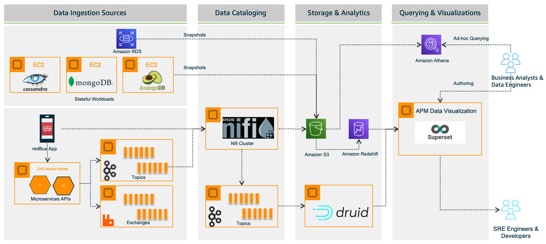
In the following sections, we look at each component in more detail.
Data ingestion sources
With the data platform 1.0, the data is ingested from various sources:
- Real time – The real-time data flows from redBus mobile apps, the backend microservices, and when a passenger, bus operator, or application does any operation like booking bus tickets, searching the bus inventory, uploading a KYC document, and more
- Batch mode – Scheduled jobs fetch data from multiple persistent data stores like Amazon Relational Database Service (Amazon RDS), where the OLTP data from all its applications are stored, Apache Cassandra clusters, where the bus inventory from various operators is stored, Arango DB, where the user identity graphs are stored, and more
Data cataloging
The real-time data is ingested into their self-managed Apache Nifi clusters, an open-source data platform that is used to clean, analyze, and catalog the data with its routing capabilities before sending the data to its destination.
Storage and analytics
redBus uses the following services for its storage and analytical needs:
- Amazon Simple Storage Service (Amazon S3), an object storage service that provides the foundation for their data lake because of its virtually unlimited scalability and higher durability. Real-time data flows from Apache Druid and data from the data stores flow at regular intervals based on the schedules.
- Apache Druid, an OLAP-style data store (data flows via Kafka Druid data loader), which computes facts and metrics against various dimensions during the data loading process.
- Amazon Redshift, a cloud data warehouse service that helps you analyze exabytes of data and run complex analytical queries. redBus uses Amazon Redshift to store the processed data from Amazon S3 and the aggregated data from Apache Druid.
Querying and visualization
To make redBus as data-driven as possible, they ensured that the data is accessible to their SRE engineers, data engineers, and business analysts via a visualization layer. This layer features dashboards being served using Apache SuperSet, an open-source data visualization application, and Amazon Athena, an interactive query service to analyze data in Amazon S3 using standard SQL for ad hoc querying requirements.
The challenges
Initially, redBus handled data that was being ingested at the rate of 10 million events per day. Over time, as its business started growing, so did the data volume (from gigabytes to terabytes to petabytes), data ingestion per day (from 10 million to 320 million events), and its business intelligence dashboard needs. Soon after, they started facing challenges with their self-managed Superset’s BI capabilities, and the increased operational complexities.
Limited BI capabilities
redBus encountered the following BI limitations:
- Inability to create visualizations from multiple data sources – Superset doesn’t allow creating visualizations from multiple tables within its data exploration layer. redBus data engineers had to have the tables joined beforehand at the data source level itself. In order to create a 360-degree view for redBus’s business stakeholders, it became inconvenient for data engineers to maintain multiple tables supporting the visualization layer.
- No global filter for visuals in a dashboard – A global or primary filter across visuals in a dashboard is not supported in Superset. For example, consider there are visuals like Sales Wins by Region, YTD Revenue Realized by Region, Sales Pipeline by Region, and more in a dashboard, and a filter Region is added to the dashboard with values like EMEA, APAC, and US. The filter Region will only apply to one of the visuals, not the entire dashboard. However, dashboard users expected filtering across the dashboard.
- Not a business-user friendly tool – Superset is highly developer centric when it comes to customization. For example, if a redBus business analyst had to customize a timed refresh that automatically re-queries every slice on a dashboard according to a pre-set value, then the analyst has to update the dashboard’s JSON metadata field. Therefore, having knowledge of JSON and its syntax is mandatory for doing any customization on the visuals or dashboard.
Increased operational cost
Although Superset is open source, which means there are no licensing costs, it also means there is more effort in maintaining all the components required for it to function as an enterprise-grade BI tool. redBus has deployed and maintained a web server (Nginx) fronted by an Application Load Balancer to do the load balancing; a metadata database server (MySQL) where Superset stores its internal information like users, slices, and dashboard definitions; an asynchronous task queue (Celery) for supporting long-running queries; a message broker (RabbitMQ); and a distributed caching server (Redis) for caching the results, charting data, and more on Amazon Elastic Compute Cloud (Amazon EC2) instances. The following diagram illustrates this architecture.
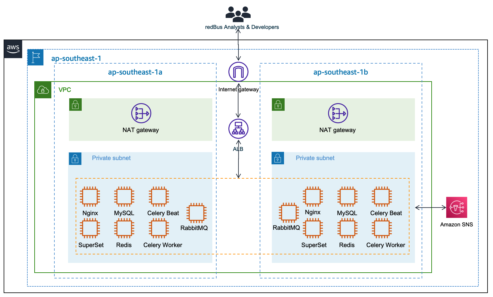
redBus’s DevOps team had to do the heavy lifting of provisioning the infrastructure, taking backups, scaling the components manually as needed, upgrading the components individually, and more. It also required a Python web developer to be around for making the configurational changes so all the components work together seamlessly. All these manual operations increased the total cost of ownership for redBus.
Journey towards QuickSight
redBus started exploring BI solutions primarily around a couple of its dashboarding requirements:
- BI dashboards for business stakeholders and analysts, where the data is sourced via Amazon S3 and Amazon Redshift.
- A real-time application performance monitoring (APM) dashboard to help their SRE engineers and developers identify the root cause of an issue in their microservices deployment so they can fix the issues before they affect their customer’s experience. In this case, the data is sourced via Druid.
QuickSight fit into most of redBus’s BI dashboard requirements, and in no time their data platform team started with a proof of concept (POC) for a couple of their complex dashboards. At the end of the POC, which spanned a month’s time, the team shared their findings.
First, QuickSight is rich in BI capabilities, including the following:
- It’s a self-service BI solution with drag-and-drop features that could help redBus analysts comfortably use it without any coding efforts.
- Visualizations from multiple data sources in a single dashboard could help redBus business stakeholders get a 360-degree view of sales, forecasting, and insights in a single pane of glass.
- Cascading filters across visuals and across sheets in a dashboard are much-needed features for redBus’s BI requirements.
- QuickSight offers Excel-like visuals—tables with calculations, pivot tables with cell grouping, and styling are attractive for the viewers.
- The Super-fast, Parallel, In-memory Calculation Engine (SPICE) in QuickSight could help redBus scale to hundreds of thousands of users, who can all simultaneously perform fast interactive analysis across a wide variety of AWS data sources.
- Off-the-shelf ML insights and forecasting at no additional cost would allow redBus’s data science team to focus on ML models besides sales forecasting and similar models.
- Built-in row-level security (RLS) could allow redBus to grant filtered access for their viewers. For example, redBus has many business analysts who manage different countries. With RLS, each business analyst only sees data related to their assigned country within a single dashboard.
- redBus uses OneLogin as its identity provider, which supports Security Assertion Markup Language 2.0 (SAML 2.0). With the help of identity federation and single sign-on support from QuickSight, redBus could provide a simple onboarding flow for their QuickSight users.
- QuickSight offers built-in alerts and email notification capabilities.
Secondly, QuickSight is a fully managed, cloud-native, serverless BI service offering from AWS, with the following features:
- redBus engineers don’t need to focus on the heavy lifting of provisioning, scaling, and maintaining their BI solution on EC2 instances.
- QuickSight offers native integration with AWS services like Amazon Redshift, Amazon S3, and Athena, and other popular frameworks like Presto, Snowflake, Teradata, and more. QuickSight connects to most of the data sources that redBus already has except Apache Druid, because native integration with Druid was not available as of December 2022. For a complete list of the supported data sources, see Supported data sources.
The outcome
Considering all the rich features and lower total cost of ownership, redBus chose QuickSight for their BI dashboard requirements. With QuickSight, redBus’s data engineers have built a number of dashboards in no time to give insights from petabytes of data to business stakeholders and analysts. The redBus data highway evolved to bring business intelligence to a much wider audience in their organization, with better performance and faster time-to-value. As of November 2022, it combines QuickSight for business users and Superset for real-time APM dashboards (at the time of writing, QuickSight doesn’t offer a native connector to Druid), as shown in the following diagram.
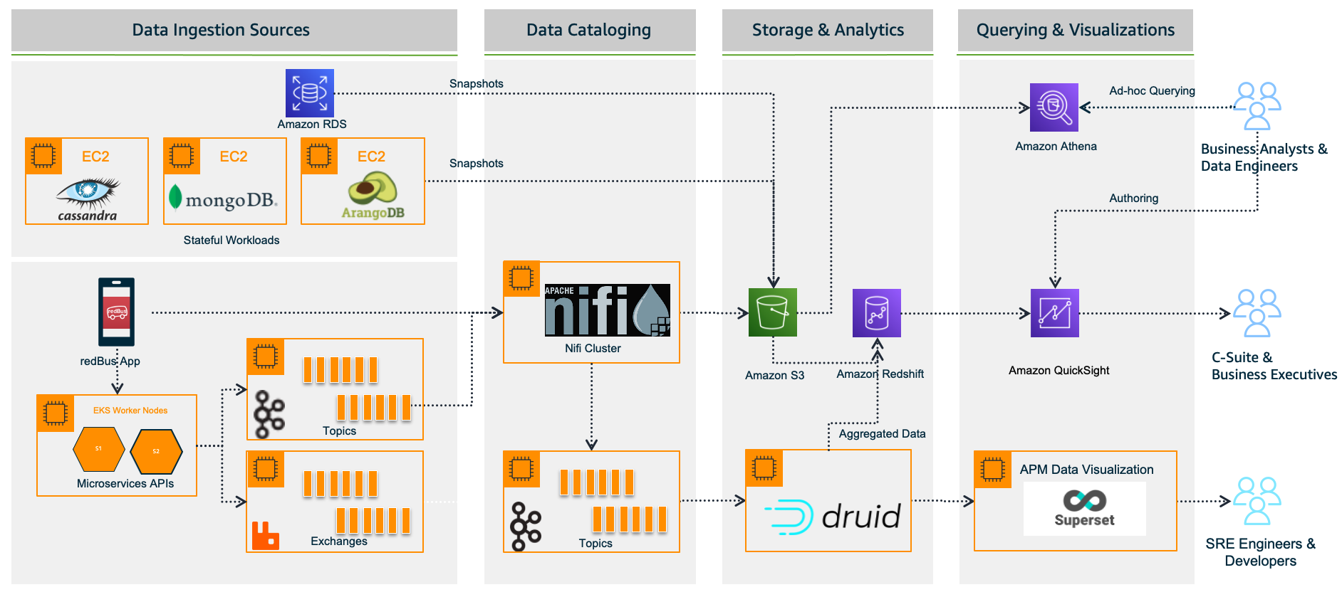
Sales anomaly detection dashboard
Although there are many dashboards that redBus deployed to production, sales anomaly detection is one of the interesting dashboards that redBus built. It uses redBus’s proprietary sales forecasting model, which in turn is sourced by historical sales data from Amazon Redshift tables and real-time sales data from Druid tables, as shown in the following figure.
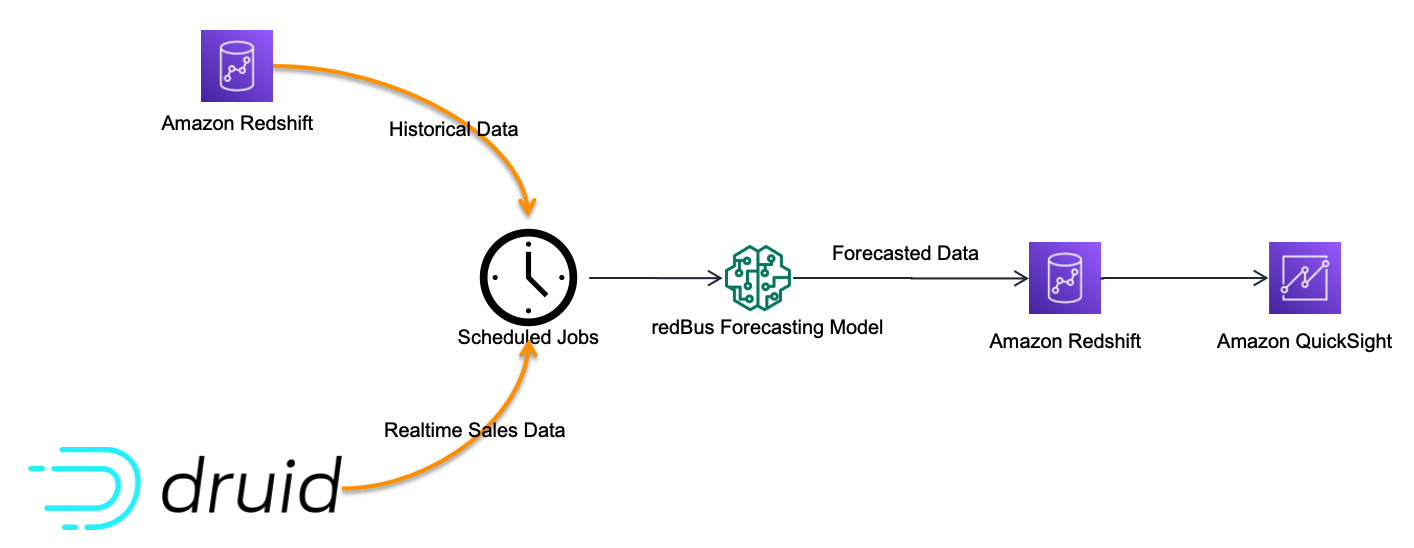
At regular intervals, the scheduled jobs feed the redBus forecasting model with real-time and historical sales data, and then the forecasted data is pushed into an Amazon Redshift table. The sales anomaly detection dashboard in QuickSight is served by the resultant Amazon Redshift table.
The following is one of the visuals from the sales anomaly detection dashboard. It’s built using a line chart representing hourly actual sales, predicted sales, and an alert threshold for a time series for a particular business cohort in redBus.
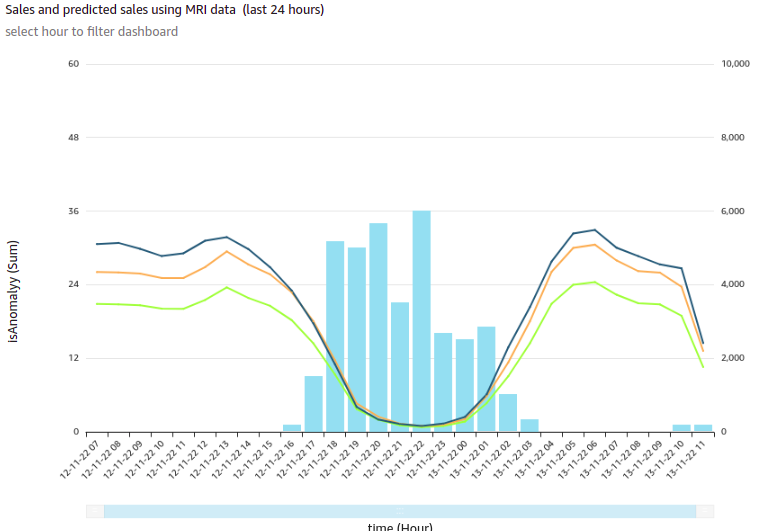
In this visual, each bar represents the number of sales anomalies triggered at a particular point in the time series.
redBus’s analysts could further drill down to the sales details and anomalies at the minute level, as shown in the following diagram. This drill-down feature comes out of the box with QuickSight.

For more details on adding drill-downs to QuickSight dashboard visuals, see Adding drill-downs to visual data in Amazon QuickSight.
Apart from the visuals, it has become one of viewers’ favorite dashboards at redBus due to the following notable features:
- Because filtering across visuals is an out-of-the-box feature in QuickSight, a timestamp-based filter is added to the dashboard. This helps in filtering multiple visuals in the dashboard in a single click.
- URL actions configured on the visuals help the viewers navigate to the context-sensitive in-house applications.
- Email alerts configured on KPIs and Gauge visuals help the viewers get notifications on time.
Next steps
Apart from building new dashboards for their BI dashboard needs, redBus is taking the following next steps:
- Exploring QuickSight Embedded Analytics for a couple of their application requirements to accelerate time to insights for users with in-context data visuals, interactive dashboards, and more directly within applications
- Exploring QuickSight Q, which could enable their business stakeholders to ask questions in natural language and receive accurate answers with relevant visualizations that can help them gain insights from the data
- Building a unified dashboarding solution using QuickSight covering all their data sources as integrations become available
Conclusion
In this post, we showed you how redBus built its data platform using various AWS services and Apache frameworks, the challenges the platform went through (especially in their BI dashboard requirements and challenges while scaling), and how they used QuickSight and lowered the total cost of ownership.
To know more about engineering at redBus, check out their medium blog posts. To learn more about what is happening in QuickSight or if you have any questions, reach out to the QuickSight Community, which is very active and offers several resources.
About the Authors
 Girish Kumar Chidananda works as a Senior Engineering Manager – Data Engineering at redBus, where he has been building various data engineering applications and components for redBus for the last 5 years. Prior to starting his journey in the IT industry, he worked as a Mechanical and Control systems engineer in various organizations, and he holds an MS degree in Fluid Power Engineering from University of Bath.
 Kayalvizhi Kandasamy works with digital-native companies to support their innovation. As a Senior Solutions Architect (APAC) at Amazon Web Services, she uses her experience to help people bring their ideas to life, focusing primarily on microservice architectures and cloud-native solutions using AWS services. Outside of work, she likes playing chess and is a FIDE rated chess player. She also coaches her daughters the art of playing chess, and prepares them for various chess tournaments.
In modern data architectures, datasets are combined across an organization using a variety of purpose-built services to unlock insights. As a result, data governance becomes a key component for data consumers and producers to know that their data-driven decisions are based on trusted and accurate datasets. One aspect of data governance is data lineage, which captures the flow of data as it goes through various systems and allows consumers to understand how a dataset was derived.
In order to capture data lineage consistently across various analytical services, you need to use a common lineage model and a robust job orchestration that is able to tie together diverse data flows. One possible solution is the open-source OpenLineage project. It provides a technology-agnostic metadata model for capturing data lineage and integrates with widely used tools. For job orchestration, it integrates with Apache Airflow, which you can run on AWS conveniently through the managed service Amazon Managed Workflows for Apache Airflow (Amazon MWAA). OpenLineage provides a plugin for Apache Airflow that extracts data lineage from Directed Acyclic Graphs (DAGs).
In this post, we show how to get started with data lineage on AWS using OpenLineage. We provide a step-by-step configuration guide for the openlineage-airflow plugin on Amazon MWAA. Additionally, we share an AWS Cloud Development Kit (AWS CDK) project that deploys a pre-configured demo environment for evaluating and experiencing OpenLineage first-hand.
OpenLineage on Apache Airflow
In the following example, Airflow turns OLTP data into a star schema on Amazon Redshift Serverless.
After staging and preparing source data from Amazon Simple Storage Service (Amazon S3), fact and dimension tables are eventually created. For this, Airflow orchestrates the execution of SQL statements that create and populate tables on Redshift Serverless.

The openlineage-airflow plugin collects metadata about creation of datasets and dependencies between them. This allows us to move from a jobs-centric approach of Airflow to a datasets-centric approach, improving the observability of workflows.
The following screenshot shows parts of the captured lineage for the previous example. It’s displayed in Marquez, an open-source metadata service for collection and visualization of data lineage with support for the OpenLineage standard. In Marquez, you can analyze the upstream datasets and transformations that eventually create the user dimension table on the right.

The example in this post is based on SQL and Amazon Redshift. OpenLineage also supports other transformation engines and data stores such as Apache Spark and dbt.
Solution overview
The following diagram shows the AWS setup required to capture data lineage using OpenLineage.
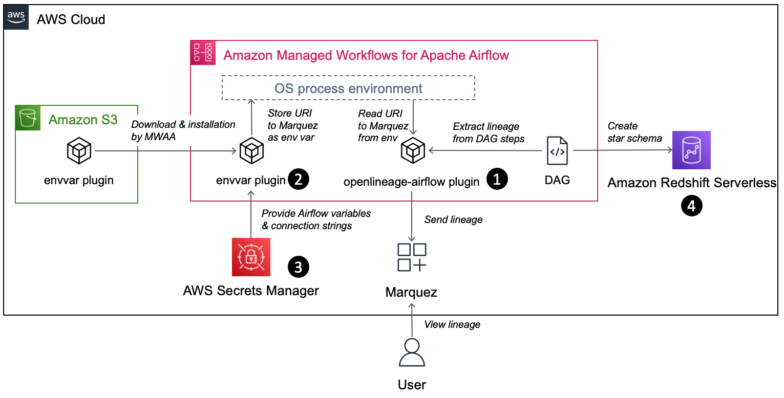
The workflow includes the following components:
- The openlineage-airflow plugin is configured on Airflow as a lineage backend. Metadata about the DAG runs is passed by Airflow core to the plugin, which converts it into OpenLineage format and sends it to an external metadata store. In our demo setup, we use Marquez as the metadata store.
- The openlineage-airflow plugin receives its configuration from environment variables. To populate these variables on Amazon MWAA, a custom Airflow plugin is used. First, the plugin reads source values from AWS Secrets Manager. Then, it creates environment variables.
- Secrets Manager is configured as a secrets backend. Typically, this type of configuration is stored in Airflow’s native metadata database. However, this approach has limitations. For instance, in case of multiple Airflow environments, you need to track and store credentials across multiple environments, and updating credentials requires you to update all the environments. With a secrets backend, you can centralize configuration.
- For demo purposes, we collect data lineage from a data pipeline, which creates a star schema in Redshift Serverless.
In the following sections, we walk you through the steps for end-to-end configuration.
Install the openlineage-airflow plugin
Specify the following dependency in the requirements.txt file of the Amazon MWAA environment. Note that the latest Airflow version currently available on Amazon MWAA is 2.4.3; for this post, use the compatible version 0.19.2 of the plugin:
For more details on installing Python dependencies on Amazon MWAA, refer to Installing Python dependencies.
For Airflow < 2.3, configure the plugin’s lineage backend through the following configuration overrides on the Amazon MWAA environment and load it immediately at Airflow start by disabling lazy load of plugins:
For more information on configuration overrides, refer to Configuration options overview.
Configure the Secrets Manager backend with Amazon MWAA
Using Secrets Manager as a secrets backend for Amazon MWAA is straightforward. First, provide the execution role of Amazon MWAA with read permission to Secrets Manager. You can use the following policy template as a starting point:
Second, configure Secrets Manager as a backend in Amazon MWAA through the following configuration overrides:
For more information configuring a secrets backend in Amazon MWAA, refer to Configuring an Apache Airflow connection using a Secrets Manager secret and Move your Apache Airflow connections and variables to AWS Secrets Manager.
Deploy a custom envvar plugin to Amazon MWAA
Apache Airflow has a built-in plugin manager through which it can be extended with custom functionality. In our case, this functionality is to populate OpenLineage-specific environment variables based on values in Secrets Manager. Natively, Amazon MWAA allows environment variables with the prefix AIRFLOW\_\_, but the openlineage-airflow plugin expects the prefix OPENLINEAGE\_\_.
The following Python code is used in the plugin. We assume the file is called envvar\_plugin.py:
Amazon MWAA has a mechanism to install a plugin through a zip archive. You zip your code, upload the archive to an S3 bucket, and pass the URL to the file to Amazon MWAA:
Upload plugins.zip to an S3 bucket and configure the URL in Amazon MWAA. The following screenshot shows the configuration via the Amazon MWAA console.

For more information on installing custom plugins on Amazon MWAA, refer to Creating a custom plugin that generates runtime environment variables.
Configure connectivity between the openlineage-airflow plugin and Marquez
As a last step, store the URL to Marquez in Secrets Manager. For this, create a secret called airflow/variables/OPENLINEAGE\_URL with value <protocol>://<hostname/ip>:<port> (for example, https://marquez.mysite.com:5000).

In case you need to spin up Marquez on AWS, you have multiple options to host, including running it on Amazon Elastic Kubernetes Service (Amazon EKS) or Amazon Elastic Compute Cloud (Amazon EC2). Refer to Running Marquez on AWS or check out our infrastructure template in the next section to deploy Marquez on AWS.
Deploy with an AWS CDK-based solution template
Assuming you want to set up a demo infrastructure for all of the above in one step, you can use the following template based on the AWS CDK.
The template has the following prerequisites:
- An AWS account.
- Amazon Linux 2 with AWS CDK, Docker CLI, and Python3 installed. Alternatively, setting up an AWS Cloud9 environment will satisfy this requirement.
Complete the following steps to deploy the template:
- Clone GitHub repository and install Python dependencies. Bootstrap the AWS CDK if required.
- Update the value for the variable
EXTERNAL\_IPinconstants.pyto your outbound IP for connecting to the internet:This configures security groups so that you can access Marquez but block other clients.
constants.pyis found in the root folder of the cloned repository. - Deploy the VPC\_S3 stack to provision a new VPC dedicated for this solution as well as the security groups that are used by the different components:
It creates a new S3 bucket and uploads the source raw data based on the TICKIT sample database. This serves as the landing area from the OLTP database. We then need to parse the metadata of these files through an AWS Glue crawler, which facilitates the native integration between Amazon Redshift and the S3 data lake.
- Deploy the lineage stack to create an EC2 instance that hosts Marquez:
Access the Marquez web UI through
https://{ec2.public\_dns\_name}:3000/. This URL is also available as part of the AWS CDK outputs for the lineage stack. - Deploy the Amazon Redshift stack to create a Redshift Serverless endpoint:
- Deploy the Amazon MWAA stack to create an Amazon MWAA environment:
You can access the Amazon MWAA UI through the URL provided in the AWS CDK output.
Test a sample data pipeline
On Amazon MWAA, you can see an example data pipeline deployed that consists of two DAGs. It builds a star schema on top of the TICKIT sample database. One DAG is responsible for loading data from the S3 data lake into an Amazon Redshift staging layer; the second DAG loads data from the staging layer to the dimensional model.

Open the Amazon MWAA UI through the URL obtained in the deployment steps and launch the following DAGs: rs\_source\_to\_staging and rs\_staging\_to\_dm. As part of the run, the lineage metadata is sent to Marquez.
After the DAG has been run, open the Marquez URL obtained in the deployment steps. In Marquez, you can find the lineage metadata for the computed star schema and related data assets on Amazon Redshift.
Clean up
Delete the AWS CDK stacks to avoid ongoing charges for the resources that you created. Run the following command in the aws-mwaa-openlineage project directory so that all resources are undeployed:
Summary
In this post, we showed you how to automate data lineage with OpenLineage on Amazon MWAA. As part of this, we covered how to install and configure the openlineage-airflow plugin on Amazon MWAA. Additionally, we provided a ready-to-use infrastructure template for a complete demo environment.
We encourage you to explore what else can be achieved with OpenLineage. A job orchestrator like Apache Airflow is only one piece of a data platform and not all possible data lineage can be captured on it. We recommend exploring OpenLineage’s integration with other platforms like Apache Spark or dbt. For more information, refer to Integrations.
Additionally, we recommend you visit the AWS Big Data Blog for other useful blog posts on Amazon MWAA and data governance on AWS.
About the Authors
 Stephen Said is a Senior Solutions Architect and works with Digital Native Businesses. His areas of interest are data analytics, data platforms and cloud-native software engineering.
 Vishwanatha Nayak is a Senior Solutions Architect at AWS. He works with large enterprise customers helping them design and build secure, cost-effective, and reliable modern data platforms using the AWS cloud. He is passionate about technology and likes sharing knowledge through blog posts and twitch sessions.
 Paul Villena is an Analytics Solutions Architect with expertise in building modern data and analytics solutions to drive business value. He works with customers to help them harness the power of the cloud. His areas of interests are infrastructure-as-code, serverless technologies and coding in Python.
With AWS Lake Formation, you can build data lakes with multiple AWS accounts in a variety of ways. For example, you could build a data mesh, implementing a centralized data governance model and decoupling data producers from the central governance. Such data lakes enable the data as an asset paradigm and unleash new possibilities with data discovery and exploration across organization-wide consumers. While enabling the power of data in decision-making across your organization, it’s also crucial to secure the data. With Lake Formation, sharing datasets across accounts only requires a few simple steps, and you can control what you share.
Lake Formation has launched Version 3 capabilities for sharing AWS Glue Data Catalog resources across accounts. When moving to Lake Formation cross-account sharing V3, you get several benefits. When moving from V1, you get more optimized usage of AWS Resource Access Manager (AWS RAM) to scale sharing of resources. When moving from V2, you get a few enhancements. First, you don’t have to maintain AWS Glue resource policies to share using LF-tags because Version 3 uses AWS RAM. Second, you can share with AWS Organizations using LF-tags. Third, you can share to individual AWS Identity and Access Management (IAM) users and roles in other accounts, thereby providing data owners control over which individuals can access their data.
Lake Formation tag-based access control (LF-TBAC) is an authorization strategy that defines permissions based on attributes called LF-tags. LF-tags are different from IAM resource tags and are associated only with Lake Formation databases, tables, and columns. LF-TBAC allows you to define the grant and revoke permissions policy by grouping Data Catalog resources, and therefore helps in scaling permissions across a large number of databases and tables. LF-tags are inherited from a database to all its tables and all the columns of each table.
Version 3 offers the following benefits:
- True central governance with cross-account sharing to specific IAM principals in the target account
- Ease of use in not having to maintain an AWS Glue resource policy for LF-TBAC
- Efficient reuse of AWS RAM shares
- Ease of use in scaling to hundreds of accounts with LF-TBAC
In this post, we illustrate the new features of cross-account sharing Version 3 in a producer-consumer scenario using TPC datasets. We walk through the setup of using LF-TBAC to share data catalog resources from the data producer account to direct IAM users in the consumer account. We also go through the steps in the receiving account to accept the shares and query the data.
Solution overview
To demonstrate the Lake Formation cross-account Version 3 features, we use the TPC datasets available at s3://aws-data-analytics-workshops/shared\_datasets/tpcparquet/. The solution consists of steps in both accounts.
In account A, complete the following steps:
- As a data producer, register the dataset with Lake Formation and create AWS Glue Data Catalog tables.
- Create LF-tags and associate them with the database and tables.
- Grant LF-tag based permissions on resources directly to personas in consumer account B.
The following steps take place in account B:
- The consumer account data lake admin reviews and accepts the AWS RAM invitations.
- The data lake admin gives CREATE DATABASE access to the IAM user
lf\_business\_analysts. - The data lake admin creates a database for the marketing team and grants CREATE TABLE access to
lf\_campaign\_manager. - The IAM users create resource links on the shared database and tables and query them in Amazon Athena.
The producer account A has the following personas:
- Data lake admin – Manages the data lake in the producer account
- lf-producersteward – Manages the data and user access
The consumer account B has the following personas:
- Data lake admin – Manages the data lake in the consumer account
- lf-business-analysts – The business analysts in the sales team needs access to non-PII data
- lf-campaign-manager – The manager in the marketing team needs access to data related to products and promotions
Prerequisites
You need the following prerequisites:
- Two AWS accounts. For this demonstration of how AWS RAM invites are created and accepted, you should use two accounts that are not part of the same organization.
- An admin IAM user in both accounts to launch the AWS CloudFormation stacks.
- Lake Formation mode enabled in both the producer and consumer account with cross-account Version 3. For instructions, refer to Change the default permission model.
Lake Formation and AWS CloudFormation setup in account A
To keep the setup simple, we have an IAM admin registered as the data lake admin.
- Sign into the AWS Management Console in the
us-east-1Region. - On the Lake Formation console, under Permissions in the navigation pane, choose Administrative roles and tasks.
- Select Choose Administrators under Datalake administrators.
- In the pop-up window Manage data lake administrators, under IAM users and roles, choose IAM admin user and choose Save.
- Choose Launch Stack to deploy the CloudFormation template:
- Choose Next.
- Provide a name for the stack and choose Next.
- On the next page, choose Next.
- Review the details on the final page and select I acknowledge that AWS CloudFormation might create IAM resources.
- Choose Create.
Stack creation should take about 2–3 minutes. The stack establishes the producer setup as follows:
- Creates an Amazon Simple Storage Service (Amazon S3) data lake bucket
- Registers the data lake bucket with Lake Formation
- Creates an AWS Glue database and tables
- Creates an IAM user (
lf-producersteward) who will act as producer steward - Creates LF-tags and assigns them to the created catalog resources as specified in the following table
| Database | Table | LF-Tag Key | LF-Tag Value | Resource Tagged |
lftpcdb | . | Sensitivity | Public | DATABASE |
lftpcdb | items | HasCampaign | true | TABLE |
lftpcdb | promotions | HasCampaign | true | TABLE |
lftpcdb | customers table columns = "c\_last\_name","c\_first\_name","c\_email\_address" | Sensitivity | Confidential | TABLECOLUMNS |
Verify permissions in account A
After the CloudFormation stack launches, complete the following steps in account A:
- On the AWS CloudFormation console, navigate to the Outputs tab of the stack.

- Choose the
LFProducerStewardCredentialsvalue to navigate to the AWS Secrets Manager console. - In the Secret value section, choose Retrieve secret value.
- Note down the secret value for the password for IAM user
lf-producersteward.
You need this to log in to the console later as the user lf-producersteward.

- On the LakeFormation console, choose Databases on the navigation pane.
- Open the database
lftpcdb. - Verify the LF-tags on the database are created.

- Choose View tables and choose the
itemstable to verify the LF-tags.

- Repeat the steps for the
promotionsandcustomerstables to verify the LF-tags assigned.


- On the Lake Formation console, under Data catalog in the navigation pane, choose Databases.
- Select the database
lftpcdband on the Actions menu, choose View Permissions. - Verify that there are no default permissions granted on the database
lftpcdbforIAMAllowedPrincipals. - If you find any, select the permission and choose Revoke to revoke the permission.
- On the AWS Management Console, choose the AWS CloudShell icon on the top menu.

This opens AWS CloudShell in another tab of the browser. Allow a few minutes for the CloudShell environment to set up.
- Run the following AWS Command Line Interface (AWS CLI) command after replacing
{BUCKET\_NAME}withDataLakeBucketfrom the stack output.
If CloudShell isn’t available in your chosen Region, run the following AWS CLI command to copy the required dataset from your preferred AWS CLI environment as the IAM admin user.
- Verify that your S3 bucket has the dataset copied in it.
- Log out as the IAM admin user.
Grant permissions in account A
Next, we continue granting Lake Formation permissions to the dataset as a data steward within the producer account. The data steward grants the following LF-tag-based permissions to the consumer personas.
| Consumer Persona | LF-tag Policy |
lf-business-analysts | Sensitivity=Public |
lf-campaign-manager | HasCampaign=true |
- Log in to account A as user
lf-producersteward, using the password you noted from Secrets Manager earlier. - On the Lake Formation console, under Permissions in the navigation pane, choose Data Lake permissions.
- Choose Grant.
- Under Principals, select External accounts.
- Provide the ARN of the IAM user in the consumer account (
arn:aws:iam::<accountB\_id>:user/lf-business-analysts) and press Enter.

- Under LF\_Tags or catalog resources, select Resources matched by LF-Tags.
- Choose Add LF-Tag to add a new key-value pair.
- For the key, choose
Sensitivityand for the value, choosePublic. - Under Database permissions, select Describe, and under Table permissions, select Select and Describe.

- Choose Grant to apply the permissions.
- On the Lake Formation console, under Permissions in the navigation pane, choose Data Lake permissions.
- Choose Grant.
- Under Principals, select External accounts.
- Provide the ARN of the IAM user in the consumer account (
arn:aws:iam::<accountB\_id>:user/lf-campaign-manager) and press Enter. - Under LF\_Tags or catalog resources, select Resources matched by LF-Tags.
- Choose Add LF-Tag to add a new key-value pair.
- For the key, choose
HasCampaignand for the value, choose true.

- Under Database permissions, select Describe, and under Table permissions, select Select and Describe.
- Choose Grant to apply the permissions.
- Verify on the Data lake permissions tab that the permissions you have granted show up correctly.

AWS CloudFormation setup in account B
Complete the following steps in the consumer account:
- Log in as an IAM admin user in account B and launch the CloudFormation stack:
- Choose Next.
- Provide a name for the stack, then choose Next.
- On the next page, choose Next.
- Review the details on the final page and select I acknowledge that AWS CloudFormation might create IAM resources.
- Choose Create.
Stack creation should take about 2–3 minutes. The stack sets up the following resources in account B:
- IAM users
datalakeadmin1,lf-business-analysts, andlf-campaign-manager, with relevant IAM and Lake Formation permissions - A database called
db\_for\_shared\_tableswithCreate\_Tablepermissions to the lf-campaign-manager user - An S3 bucket named
lfblog-athenaresults-<your-accountB-id>-us-east-1 with ListBucketand write permissions tolf-business-analystsandlf-campaign-manager
Note down the stack output details.

Accept resource shares in account B
After you launch the CloudFormation stack, complete the following steps in account B:
- On the CloudFormation stack Outputs tab, choose the link for
DataLakeAdminCredentials.
This takes you to the Secrets Manager console.
- On the Secrets Manager console, choose Retrieve secret value and copy the password for
DataLakeAdminuser. - Use the
ConsoleIAMLoginURLvalue from the CloudFormation template output to log in to account B with the data lake admin user name datalakeadmin1 and the password you copied from Secrets Manager. - Open the AWS RAM console in another browser tab.
- In the navigation pane, under Shared with me, choose Resource shares to view the pending invitations.
You should see two resource share invitations from the producer account A: one for database-level share and one for table-level share.

- Choose each resource share link, review the details, and choose Accept.
After you accept the invitations, the status of the resource shares changes from Active from Pending.
Grant permissions in account B
To grant permissions in account B, complete the following steps:
- On the Lake Formation console, under Permissions on the navigation pane, choose Administrative roles and tasks.

- Under Database creators, choose Grant.

- Under IAM users and roles, choose
lf-business-analysts. - For Catalog permissions, select Create database.
- Choose Grant.
- Log out of the console as the data lake admin user.
Query the shared datasets as consumer users
To validate the lf-business-analysts user’s data access, perform the following steps:
- Log in to the console as lf-business-analysts, using the credentials noted from the CloudFormation stack output.
- On the Lake Formation console, under Data catalog in the navigation pane, choose Databases.

- Select the database
lftpcdband on the Actions menu, choose Create resource link.

- Under Resource link name, enter
rl\_lftpcdb. - Choose Create.
- After the resource link is created, select the resource link and choose View tables.
You can now see the four tables in the shared database.

- Open the Athena console in another browser tab and choose the
lfblog-athenaresults-<your-accountB-id>-us-east-1 bucketas the query results location. - Verify data access using the following query (for more information, refer to Running SQL queries using Amazon Athena):
The following screenshot shows the query output.

Notice that account A shared the database lftpcdb to account B using the LF-tag expression Sensitivity=Public. Columns c\_first\_name, c\_last\_name, and c\_email\_address in table customers were overwritten with Sensitivity=Confidential. Therefore, these three columns are not visible to user lf-business-analysts.
You can preview the other tables from the database similarly to see the available columns and data.
- Log out of the console as
lf-business-analysts.
Now we can validate the lf-campaign-manager user’s data access.
- Log in to the console as lf-campaign-manager using the credentials noted from the CloudFormation stack output.
- On the Lake Formation console, under Data catalog in the navigation pane, choose Databases.
- Verify that you can see the database
db\_for\_shared\_tablesshared by the data lake admin.

- Under Data catalog in the navigation pane, choose Tables.
You should be able to see the two tables shared from account A using the LF-tag expression HasCampaign=true. The two tables show the Owner account ID as account A.

Because lf-campaign-manager received table level shares, this user will create table-level resource links for querying in Athena.
- Select the promotions table, and on the Actions menu, choose Create resource link.

- For Resource link name, enter
rl\_promotions.

- Under Database, choose
db\_for\_shared\_tablesfor the database to contain the resource link. - Choose Create.
- Repeat the table resource link creation for the other table items.
Notice that the resource links show account B as owner, whereas the actual tables show account A as the owner.

- Open the Athena console in another browser tab and choose the
lfblog-athenaresults-<your-accountB-id>-us-east-1bucket as the query results location. - 11. Query the tables using the resource links.
As shown in the following screenshot, all columns of both tables are accessible to lf-campaign-manager.

In summary, you have seen how LF-tags are used to share a database and select tables from one account to another account’s IAM users.
Clean up
To avoid incurring charges on the AWS resources created in this post, you can perform the following steps.
First, clean up resources in account A:
- Empty the S3 bucket created for this post by deleting the downloaded objects from your S3 bucket.
- Delete the CloudFormation stack.
This deletes the S3 bucket, custom IAM roles, policies, and the LF database, tables, and permissions.
- You may choose to undo the Lake Formation settings also and add IAM access back from the Lake Formation console Settings page.
Now complete the following steps in account B:
- Empty the S3 bucket
lfblog-athenaresults-<your-accountB-id>-us-east-1used as the Athena query results location. - Revoke permission to
lf-business-analystsas database creator. - Delete the CloudFormation stack.
This deletes the IAM users, S3 bucket, Lake Formation database db\_for\_shared\_tables, resource links, and all the permissions from Lake Formation.
If there are any resource links and permissions left, delete them manually in Lake Formation from both accounts.
Conclusion
In this post, we illustrated the benefits of using Lake Formation cross-account sharing Version 3 using LF-tags to direct IAM principals and how to receive the shared tables in the consumer account. We used a two-account scenario in which a data producer account shares a database and specific tables to individual IAM users in another account using LF-tags. In the receiving account, we showed the role played by a data lake admin vs. the receiving IAM users. We also illustrated how to overwrite column tags to mask and share PII data.
With Version 3 of cross-account sharing features, Lake Formation makes possible more modern data mesh models, where a producer can directly share to an IAM principal in another account, instead of the entire account. Data mesh implementation becomes easier for data administrators and data platform owners because they can easily scale to hundreds of consumer accounts using the LF-tags based sharing to organizational units or IDs.
We encourage you to upgrade your Lake Formation cross-account sharing to Version 3 and benefit from the enhancements. For more details, see Updating cross-account data sharing version settings.
About the authors
 Aarthi Srinivasan is a Senior Big Data Architect with AWS Lake Formation. She likes building data lake solutions for AWS customers and partners. When not on the keyboard, she explores the latest science and technology trends and spends time with her family.
 Srividya Parthasarathy is a Senior Big Data Architect on the AWS Lake Formation team. She enjoys building analytics and data mesh solutions on AWS and sharing them with the community.
This post was cowritten with Babu Srinivasan and Robert Walters from MongoDB.
Amazon Managed Streaming for Apache Kafka (Amazon MSK) is a fully managed, highly available Apache Kafka service. Amazon MSK makes it easy to ingest and process streaming data in real time and use that data easily within the AWS ecosystem. With Amazon MSK Serverless, you can automatically provision and manage required resources to provide on-demand streaming capacity and storage for your applications.
Amazon MSK also supports integration of data sources such as MongoDB Atlas via Amazon MSK Connect. MSK Connect allows serverless integration of MongoDB data with Amazon MSK using the MongoDB Connector for Apache Kafka.
MongoDB Atlas Serverless provides database services that dynamically scale up and down with data size and throughput—and the cost scales accordingly. It’s best suited for applications with variable demands to be managed with minimal configuration. It provides high performance and reliability with automated upgrade, encryption, security, metrics, and backup features built in with the MongoDB Atlas infrastructure.
MSK Serverless is a type of cluster for Amazon MSK. Just like MongoDB Atlas Serverless, MSK Serverless automatically provisions and scales compute and storage resources. You can now create end-to-end serverless workflows. You can build a serverless streaming pipeline with serverless ingestion using MSK Serverless and serverless storage using MongoDB Atlas. In addition, MSK Connect now supports private DNS hostnames. This allows Serverless MSK instances to connect to Serverless MongoDB clusters via AWS PrivateLink, providing you with secure connectivity between platforms.
If you’re interested in using a non-serverless cluster, refer to Integrating MongoDB with Amazon Managed Streaming for Apache Kafka (MSK).
This post demonstrates how to implement a serverless streaming pipeline with MSK Serverless, MSK Connect, and MongoDB Atlas.
Solution overview
The following diagram illustrates our solution architecture.

The data flow starts with an Amazon Elastic Compute Cloud (Amazon EC2) client instance that writes records to an MSK topic. As data arrives, an instance of the MongoDB Connector for Apache Kafka writes the data to a collection in the MongoDB Atlas Serverless cluster. For secure connectivity between the two platforms, an AWS PrivateLink connection is created between the MongoDB Atlas cluster and the VPC containing the MSK instance.
This post walks you through the following steps:
- Create the serverless MSK cluster.
- Create the MongoDB Atlas Serverless cluster.
- Configure the MSK plugin.
- Create the EC2 client.
- Configure an MSK topic.
- Configure the MongoDB Connector for Apache Kafka as a sink.
Configure the serverless MSK cluster
To create a serverless MSK cluster, complete the following steps:
- On the Amazon MSK console, choose Clusters in the navigation pane.
- Choose Create cluster.
- For Creation method, select Custom create.
- For Cluster name, enter
MongoDBMSKCluster. - For Cluster type¸ select Serverless.
- Choose Next.

- On the Networking page, specify your VPC, Availability Zones, and corresponding subnets.
- Note the Availability Zones and subnets to use later.

- Choose Next.
- Choose Create cluster.
When the cluster is available, its status becomes Active.

Create the MongoDB Atlas Serverless cluster
To create a MongoDB Atlas cluster, follow the Getting Started with Atlas tutorial. Note that for the purposes of this post, you need to create a serverless instance.

After the cluster is created, configure an AWS private endpoint with the following steps:
- On the Security menu, choose Network Access.

- On the Private Endpoint tab, choose Serverless Instance.

- Choose Create new endpoint.
- For Serverless Instance, choose the instance you just created.
- Choose Confirm.

- Provide your VPC endpoint configuration and choose Next.

- When creating the AWS PrivateLink resource, make sure you specify the exact same VPC and subnets that you used earlier when creating the networking configuration for the serverless MSK instance.
- Choose Next.

- Follow the instructions on the Finalize page, then choose Confirm after your VPC endpoint is created.
Upon success, the new private endpoint will show up in the list, as shown in the following screenshot.

Configure the MSK Plugin
Next, we create a custom plugin in Amazon MSK using the MongoDB Connector for Apache Kafka. The connector needs to be uploaded to an Amazon Simple Storage Service (Amazon S3) bucket before you can create the plugin. To download the MongoDB Connector for Apache Kafka, refer to Download a Connector JAR File.
- On the Amazon MSK console, choose Customized plugins in the navigation pane.
- Choose Create custom plugin.
- For S3 URI, enter the S3 location of the downloaded connector.
- Choose Create custom plugin.

Configure an EC2 client
Next, let’s configure an EC2 instance. We use this instance to create the topic and insert data into the topic. For instructions, refer to the section Configure an EC2 client in the post Integrating MongoDB with Amazon Managed Streaming for Apache Kafka (MSK).
Create a topic on the MSK cluster
To create a Kafka topic, we need to install the Kafka CLI first.
- On the client EC2 instance, first install Java:
sudo yum install java-1.8.0
- Next, run the following command to download Apache Kafka:
wget https://archive.apache.org/dist/kafka/2.6.2/kafka\_2.12-2.6.2.tgz
- Unpack the tar file using the following command:
tar -xzf kafka\_2.12-2.6.2.tgz
The distribution of Kafka includes a bin folder with tools that can be used to manage topics.
- Go to the
kafka\_2.12-2.6.2directory and issue the following command to create a Kafka topic on the serverless MSK cluster:
bin/kafka-topics.sh --create --topic sandbox\_sync2 --bootstrap-server <BOOTSTRAP SERVER> --command-config=bin/client.properties --partitions 2
You can copy the bootstrap server endpoint on the View Client Information page for your serverless MSK cluster.

You can configure IAM authentication by following these instructions.
Configure the sink connector
Now, let’s configure a sink connector to send the data to the MongoDB Atlas Serverless instance.
- On the Amazon MSK console, choose Connectors in the navigation pane.
- Choose Create connector.
- Select the plugin you created earlier.
- Choose Next.

- Select the serverless MSK instance that you created earlier.
- Enter your connection configuration as the following code:
Make sure that the connection to the MongoDB Atlas Serverless instance is through AWS PrivateLink. For more information, refer to Connecting Applications Securely to a MongoDB Atlas Data Plane with AWS PrivateLink.
- In the Access Permissions section, create an AWS Identity and Access Management (IAM) role with the required trust policy.
- Choose Next.

- Specify Amazon CloudWatch Logs as your log delivery option.
- Complete your connector.
When the connector status changes to Active, the pipeline is ready.

Insert data into the MSK topic
On your EC2 client, insert data into the MSK topic using the kafka-console-producer as follows:
To verify that data successfully flows from the Kafka topic to the serverless MongoDB cluster, we use the MongoDB Atlas UI.

If you run into any issues, be sure to check the log files. In this example, we used CloudWatch to read the events that were generated from Amazon MSK and the MongoDB Connector for Apache Kafka.

Clean up
To avoid incurring future charges, clean up the resources you created. First, delete the MSK cluster, connector, and EC2 instance:
- On the Amazon MSK console, choose Clusters in the navigation pane.
- Select your cluster and on the Actions menu, choose Delete.
- Choose Connectors in the navigation pane.
- Select your connector and choose Delete.
- Choose Customized plugins in the navigation pane.
- Select your plugin and choose Delete.
- On the Amazon EC2 console, choose Instances in the navigation pane.
- Choose the instance you created.
- Choose Instance state, then choose Terminate instance.
- On the Amazon VPC console, choose Endpoints in the navigation pane.
- Select the endpoint you created and on the Actions menu, choose Delete VPC endpoints.
Now you can delete the Atlas cluster and AWS PrivateLink:
- Log in to the Atlas cluster console.
- Navigate to the serverless cluster to be deleted.
- On the options drop-down menu, choose Terminate.

- Navigate to the Network Access section.
- Choose the private endpoint.
- Select the serverless instance.
- On the options drop-down menu, choose Terminate.

Summary
In this post, we showed you how to build a serverless streaming ingestion pipeline using MSK Serverless and MongoDB Atlas Serverless. With MSK Serverless, you can automatically provision and manage required resources on an as-needed basis. We used a MongoDB connector deployed on MSK Connect to seamlessly integrate the two services, and used an EC2 client to send sample data to the MSK topic. MSK Connect now supports Private DNS hostnames, enabling you to use private domain names between the services. In this post, the connector used the default DNS servers of the VPC to resolve the Availability Zone-specific private DNS name. This AWS PrivateLink configuration allowed secure and private connectivity between the MSK Serverless instance and the MongoDB Atlas Serverless instance.
To continue your learning, check out the following resources:
- MongoDB Kafka Connector
- Amazon MSK Serverless
- Getting started using Amazon MSK
- Getting started using MSK Connect
About the Authors
Igor Alekseev is a Senior Partner Solution Architect at AWS in Data and Analytics domain. In his role Igor is working with strategic partners helping them build complex, AWS-optimized architectures. Prior joining AWS, as a Data/Solution Architect he implemented many projects in Big Data domain, including several data lakes in Hadoop ecosystem. As a Data Engineer he was involved in applying AI/ML to fraud detection and office automation.
 Kiran Matty is a Principal Product Manager with Amazon Web Services (AWS) and works with the Amazon Managed Streaming for Apache Kafka (Amazon MSK) team based out of Palo Alto, California. He is passionate about building performant streaming and analytical services that help enterprises realize their critical use cases.
Babu Srinivasan is a Senior Partner Solutions Architect at MongoDB. In his current role, he is working with AWS to build the technical integrations and reference architectures for the AWS and MongoDB solutions. He has more than two decades of experience in Database and Cloud technologies . He is passionate about providing technical solutions to customers working with multiple Global System Integrators(GSIs) across multiple geographies.
 Robert Walters is currently a Senior Product Manager at MongoDB. Previous to MongoDB, Rob spent 17 years at Microsoft working in various roles, including program management on the SQL Server team, consulting, and technical pre-sales. Rob has co-authored three patents for technologies used within SQL Server and was the lead author of several technical books on SQL Server. Rob is currently an active blogger on MongoDB Blogs.
This post was co-written with Hardik Modi, AVP, Threat and Migitation Products at NETSCOUT.
NETSCOUT Omnis Threat Horizon is a global cybersecurity awareness platform providing users with highly contextualized visibility into “over the horizon” threat activity on the global DDoS (Distributed Denial of Service) landscape—threats that could be impacting their industry, their customers, or their suppliers. It allows visitors to create custom profiles and understand DDoS activity that is being observed in near-real time through NETSCOUT’s ATLAS visibility platform. Users can create free accounts to create customized profiles that lead to a map-based visualization (as in the following screenshot) as well as tailored summary reporting. DDoS attacks can be impactful to services delivered over the internet. Visibility of this nature is key to anyone who wishes to understand what is happening on the threat landscape. Omnis Threat Horizon has been generally available since August 2019.

To provide continuous visibility at a low per-user cost (to enable a free service), the NETSCOUT development team chose a series of AWS technologies to power the collection, storage, analysis, warehousing, user authentication, and delivery of the application. In particular, they chose Amazon OpenSearch Service as the core analytics engine. They store all processed attack records in OpenSearch Service.
This post discusses the challenges and design patterns NETSCOUT used on its path to representing the details of roughly 10 million annual DDoS attacks in near-real time.
Background
NETSCOUT, through its Arbor product line, is a long-time provider of solutions for network visibility and DDoS mitigation for service providers and enterprises. Since 2007, NETSCOUT has operated a program called ATLAS, in which customers can opt to share anonymized data about the DDoS attacks they are observing on their network. As this program has matured, NETSCOUT has comprehensive visibility into the DDoS attack landscape—both the number and nature of attacks. This visibility informs and improves their products, allowing them to share analysis findings in the form of papers, blog posts, and a biannual threat report. Since NETSCOUT started collecting and analyzing data in the current form in September 2012, they have observed 96 million attacks, allowing them to perform considerable analysis of trends across regions and verticals, as well as understand the vectors used and sizes of attacks.
Omnis Threat Horizon is a solution to display this information to a broader audience—essentially anyone interested in the threat landscape, and specifically the DDoS attack trends at any given time. In addition to providing real-time maps, the solution allows the user to go back in time to observe visually or in summary form what might have been happening at a given time.
They wanted to make sure that the visual elements and application was responsive globally, both in terms of representing real-time data as well as showing historical information. Furthermore, they wanted to keep the incremental cost per user as low as possible, in order to be able to provide this service for free globally.
Solution overview
The following diagram illustrates the solution architecture.

One of the objectives behind the chosen solution was to utilize native AWS services in every instance possible. Furthermore, they chose to break component functionality into their own microservices, and make consistent use of this through the solution.
Individual monitoring sensors deliver data to Amazon Simple Storage Service (Amazon S3) on an hourly basis. As new entries are received, Amazon Simple Notification Service (Amazon SNS) notifications are delivered, resulting in processing of the data. Successive microservices are responsible for:
- Parsing
- Running algorithms to identify and separate spurious entries
- Deduplication
- Scoring
- Confidence
After this processing, each attack is represented as a separate document in the OpenSearch Service domain. As of writing this post, NETSCOUT has approximately 96 million attacks in the cluster, all of which can be represented in some form in the maps and reports in Omnis Threat Horizon.
The data is organized in hourly bin files, and served to the application via Amazon CloudFront.
Lessons learned related to Elasticsearch
On previous projects, NETSCOUT tried Apache Cassandra, a popular NoSQL open-source database, and considered it inadequate for aggregation queries. While developing Horizon, they chose Elasticsearch to get access to more powerful aggregation query capabilities with significantly less developer time.
They started with a self-managed instance, but faced the following issues:
- Considerable expenditure of person hours simply to manage the infrastructure
- Each version upgrade was an involved process, requiring a lot of planning and still posing technical challenges along the way
- No auto scaling and big aggregation queries could break Elasticsearch
After a few cycles of powering through this, they moved to OpenSearch Service to overcome these challenges.
Outcome
NETSCOUT saw the following benefits from this architecture:
- Fast processing of attack data – The time from when attack data is received to when it is available in the data store is of the order of seconds, allowing them to provide near-real-time visibility in the solution.
- Lower management overhead – The data store grows consistently, and by using a managed service, teams avoid having to perform tasks related to cluster management. This was a big pain point with previous solutions adopted involving the same technology.
- Scalable architecture – It’s possible to add new capabilities into the pipeline as requirements emerge, without rearchitecting other components.
Conclusion
With OpenSearch Service, NETSCOUT has been able to build a resilient data store for the attack data they capture. As a result of architectural choices made and the underlying AWS services, they’re able to provide visibility into their data at small incremental costs, allowing them to provide a global visibility platform at no cost to the end-user.
With the most experience, the most reliable, scalable, and secure cloud, and the most comprehensive set of services and solutions, AWS is the best place to unlock value from your data and turn it into insight.
About the Authors

Hardik Modi is AVP, Threat and Migitation Products at NETSCOUT. In this role, he oversees the teams responsible for mitigation products as well as the creation of security content for NETSCOUTs products, enabling best-in-class protection for users, as well as the continuous delivery and publication of impactful research across the DDoS and Intrusion landscapes.

Sujatha Kuppuraju is a Principal Solutions Architect at Amazon Web Services (AWS). She engages with customers to create innovative solutions that address customer business problems and accelerate the adoption of AWS services.

Mike Arruda is a Senior Technical Account Manager at AWS, based in the New England area. He works with AWS Enterprise customers, supporting their success in adopting best practices and helping them achieve their desired business outcomes with AWS.
Many use cases are moving towards a real-time data strategy due to demand for real-time insights, low-latency response times, and the ability to adapt to the changing needs of end-users. For this type of workload, you can use Amazon Kinesis Data Streams to seamlessly provision, store, write, and read data in a streaming fashion. With Kinesis Data Streams, there are no servers to manage, and you can scale your stream to handle any additional throughput as it comes in.
Kinesis Data Streams offers 99.9% availability in a single AWS Region. For even higher availability, there are several strategies to explore within the streaming layer. This post compares and contrasts different strategies for creating a highly available Kinesis data stream in case of service interruptions, delays, or outages in the primary Region of operation.
Considerations for high availability
Before we dive into our example use case, there are several considerations to keep in mind when designing a highly available Kinesis Data Streams workload that relate to the business need for a particular pipeline:
- Recovery Time Objective (RTO) is defined by the organization. RTO is the maximum acceptable delay between the interruption of service and restoration of service. This determines what is considered an acceptable time window when service is unavailable.
- Recovery Point Objective (RPO) is defined by the organization. RPO is the maximum acceptable amount of time since the last data recovery point. This determines what is considered an acceptable loss of data between the last recovery point and the interruption of service.
In a general sense, the lower your values for RPO and RTO, the more expensive the overall solution becomes. This is because the solution needs to account for minimizing both data loss and service unavailability by having multiple instances of the service up and running in multiple Regions. This is why a big piece of high availability is the replication of data flowing through a workload. In our case, the data is replicated across Regions of Kinesis Data Streams. Conversely, the higher the RPO and RTO values are, the more complexity you introduce into your failover mechanism. This is due to the fact that the cost savings you realize by not standing up multiple instances across multiple Regions are offset by the orchestration needed to spin up these instances in the event of an outage.
In this post, we are only covering failover of a Kinesis data stream. In use cases where higher availability is required across the entire data pipeline, having failover architectures for every component (Amazon API Gateway, AWS Lambda, Amazon DynamoDB) is strongly encouraged.
The simplest approach to high availability is to start a new instance of producers, consumers, and data streams in a new Region upon service unavailability detection. The benefit here is primarily cost, but your RPO and RTO values will be higher as a result.
We cover the following strategies for highly available Kinesis Data Streams:
- Warm standby – An architecture in which there is active replication of data from the Kinesis data stream in Region A to Region B. Consumers of the data stream are running in both Regions at all times. Recommended for use cases that can’t withstand extended downtime past their replication lag.
- Cold standby – Active replication of data from the data stream in Region A to Region B, but consumers of the data stream in Region B are spun up when an outage in Region A is detected. Recommended for use cases that can afford some downtime as infrastructure is spun up in secondary Region. In this scenario, RPO will be similar to the warm standby strategy; however, RTO will increase.
For high availability purposes, these use cases need to replicate the data across Regions in a way that allows consumers and producers of the data stream to fail over quickly upon detection of a service unavailability and utilize the secondary Region’s stream. Let’s take an example architecture to further explain these DR strategies. We use API Gateway and Lambda to publish stock ticker information to a Kinesis data stream. The data is then retrieved by another Lambda consumer to save durably into DynamoDB for querying, alerting, and reporting. The following diagram illustrates this architecture.

We use this architecture with an example use case requiring the streaming workload to be highly available in the event of a Region outage. The customer can withstand an RTO of 15 minutes during an outage, because they refresh end-users’ dashboards on a 15-minute interval. The customer is sensitive to downtime and data loss, because their data will be used for historical auditing purposes, operational metrics, and dashboards for end-users. Downtime for this customer means that data isn’t able to be persisted in their database from their streaming layer, and therefore unavailable to any consuming application. For this use case, data can be retried up to 5 minutes from our Lambda function before failing over to the new Region. Consumers are considered unavailable when the stream is unavailable, and can scale up in the secondary Region to account for any backlog of events.
How might we approach making a Kinesis data stream highly available for this use case?
Warm standby pattern
The following architecture diagram illustrates the warm standby high availability pattern for Kinesis Data Streams.


The warm standby architectural pattern involves running a Kinesis data stream both in the primary and secondary Region, along with consumers and downstream destinations of the primary Region’s streaming layer being replicated as well. Sources are configured to automatically fail over to the secondary Region in the case of service unavailability in the first Region. We dive into details of how to achieve this in the client failover section of this post. Data is replicated across Regions from the data stream in the primary Region to the secondary Region. This is done instead of having the sources publish to both Regions to avoid any consistency issues between the streams in the two Regions.
Although this architectural pattern gives very high availability, it’s also the most expensive option because we’re duplicating virtually the entire streaming layer across two Regions. For business use cases that can’t withstand extended data loss or withstand downtime, this may be the best option for them. From an RTO perspective, this architectural pattern ensures there will be no downtime. There is some nuance in the RPO metric in that it depends heavily on the replication lag. In the event of the primary stream becoming unavailable, whatever data hasn’t yet been replicated may be unavailable in the secondary Region. This data won’t be considered lost, but may be unavailable for consumption until the primary stream becomes available again. This method also can result in events being out of order.
For business needs that can’t tolerate this level of record unavailability, consider retaining data on the producer for the purposes of publishing to an available stream when available, or rewinding against the source for the producer if possible so that data stuck in the primary Region can be resent to the secondary stream upon failover. We cover this consideration in the client failover section of this post.
Cold standby pattern
The following architecture diagram illustrates the cold standby high availability pattern for Kinesis Data Streams.


The cold standby architectural pattern involves running a data stream both in the primary and secondary Region, and spinning up the downstream resources like a stream consumer and destination for streams when a service interruption is detected—passive mode. Just like the warm standby pattern, sources are configured to automatically fail over to the secondary Region in the case of service unavailability in the first Region. Likewise, data is replicated across Regions from the data stream in the primary Region to the secondary Region.
The primary benefit this architectural pattern provides is cost efficiency. By not running consumers at all times, this effectively reduces your costs significantly compared to the warm standby pattern. However, this pattern may introduce some data unavailability for downstream systems while the secondary Region infrastructure is provisioned. Additionally, depending on replication lag, some records may be unavailable, as discussed in the warm standby pattern. It should be noted that depending on how long it takes to spin up resources, it may take some time for consumers to reprocess the data in the secondary Region, and latency can be introduced when failing over. Our implementation assumes a minimal replication lag and that downstream systems have the ability to reprocess a configurable amount of data to catch up to the tip of the stream. We discuss approaches to spinning these resources up in the client failover section, but one possible approach to this would be using an AWS CloudFormation template that spins these resources up on service unavailability detection.
For business needs that can tolerate some level of data unavailability and can accept interruptions while the new infrastructure in the secondary Region is spun up, this is an option to consider both from a cost perspective and an RPO/RTO perspective. The complexity of spinning up resources upon detecting service unavailability is offset by the lower cost of the overall solution.
Which pattern makes sense for our use case?
Let’s revisit the use case described earlier to identify which of the strategies best meets our needs. We can extract the pieces of information from the customer’s problem statement to identify that they need a high availability architecture that:
- Can’t withstand extended amounts of data loss
- Must resume operations within 15 minutes of service interruption identification
This criterion tells us that their RPO is close to zero, and their RTO is 15 minutes. From here, we can determine that the cold standby architecture with data replication provides us limited data loss, and the maximum downtime will be determined by the time it takes to provision consumers and downstream destinations in the secondary Region.
Let’s dive deeper into the implementation details of each of the core phases of high availability, including an implementation guide for our use case.
Launch AWS CloudFormation resources
If you want to follow along with our code samples, you can launch the following CloudFormation stack and follow the instructions in order to simulate the cold standby architecture referenced in this post.
For purposes of the Kinesis Data Streams high availability setup demo, we use us-west-2 as the primary Region and us-east-2 as the failover Region. While deploying this solution in your own account, you can choose your own primary and failover Regions.
- Deploy the supplied CloudFormation template in failover Region
us-east-2.
Make sure you specify us-east-2 as the value for the FailoverRegion parameter in the CloudFormation template.
- Deploy the supplied CloudFormation template in primary Region
us-west-2.
Make sure you specify us-east-2 as the value for the FailoverRegion parameter in the CloudFormation template.
In steps 1 and 2, we deployed the following resources in the primary and failover Regions:
- KDS-HA-Stream – AWS::Kinesis::Stream (primary and failover Region)
- KDS-HA-ProducerLambda – AWS::Lambda::Function (primary Region)
- KDS-HA-ConsumerLambda – AWS::Lambda::Function (primary and failover Region)
- KDS-HA-ReplicationAgentLambda – AWS::Lambda::Function (primary Region)
- KDS-HA-FailoverLambda – AWS::Lambda::Function (primary Region)
- ticker-prices – AWS::DynamoDB::GlobalTable (primary and failover Region)
The KDS-HA-Stream Kinesis data stream is deployed in both Regions. An enhanced fan-out consumer of the KDS-HA-Stream stream KDS-HA-ReplicationAgentLambda in the primary Region is responsible for replicating messages to the data stream in the failover Region.
KDS-HA-ConsumerLambda is a Lambda function consuming messages out of the KDS-HA-Stream stream and persisting data into a DynamoDB table after preprocessing.
You can inspect the content of the ticker-prices DynamoDB table in the primary and failover Region. Note that last\_updated\_region attribute shows us-west-2 as its value because it’s the primary Region.
Replication
When deciding how to replicate data from a data stream in Region A to a data stream in Region B, there are several strategies that involve a consumer reading data off of the primary stream and sending that data cross-Region to the secondary data stream. This would act as a replicator service, responsible for copying the data between the two streams, maintaining a relatively low latency to replicate and ensuring data isn’t lost during this replication.
Because replication off of a shared throughput data stream could impact the flow of data in a production workload, we recommend using the enhanced fan-out feature of Kinesis Data Streams consumers to ensure replication doesn’t have an impact on consumption latency.
The replication strategy implemented in this post features asynchronous replication, meaning that the replication process doesn’t block any standard data flow in the primary stream. Synchronous replication would be a safer approach to guarantee replication and avoid data loss; however, this isn’t possible without a service-side implementation.
The following image shows a timeline of data flow for the cold standby architecture, with data being replicated as soon as it’s published.

Lambda replication
Lambda can treat a Kinesis data stream as an event source, which will funnel events from your data stream into a Lambda function. This Lambda function then receives and forwards these events across Regions to your data stream in a secondary Region. Lambda functions allow you to utilize best streaming practices such as retries of records that encounter errors, bisect on error functionality, and using the Lambda parallelization factor; using more instances of your Lambda function than you have available shards can help process records faster.
This Lambda function is at the crux of the architecture for high availability; it’s responsible solely for sending data across Regions, and it also has the best capability to monitor the replication progress. Important metrics to monitor for Lambda replication include IteratorAge, which indicates how old the last record in the batch was when it finished processing. A high IteratorAge value indicates that the Lambda function is falling behind and therefore is not keeping up with data ingestion for replication purposes. A high IteratorAge can lead to a higher RPO and the higher likelihood of data unavailability when a passive failover happens.
We use the following sample Lambda function in our CloudFormation template to replicate data across Regions:
import jsonimport boto3import randomimport osimport base64def lambda\_handler(event, context): client = boto3.client("kinesis", region\_name=os.environ["FAILOVER\_REGION"]) records = [] for record in event["Records"]: records.append( { "PartitionKey": record["kinesis"]["partitionKey"], "Data": base64.b64decode(record["kinesis"]["data"]).decode("utf-8"), } ) response = client.put\_records(Records=records, StreamName="KDS-HA-Stream") if response["FailedRecordCount"] > 0: print("Failed replicating data: " + json.dumps(response)) raise Exception("Failed replicating data!")The Lambda replicator in the CloudFormation template is configured to read from the data stream in the primary Region.
The following code contains the necessary AWS Identity and Access Management (IAM) permissions for Lambda, giving access for the Lambda function to assume this role. All actions are permitted on data streams and DynamoDB. In the principal of least privilege, it’s recommended to restrict this to the necessary streams in a production environment.
AssumeRolePolicyDocument: Version: 2012-10-17 Statement: - Effect: Allow Principal: Service: - lambda.amazonaws.com Action: - 'sts:AssumeRole' Path: / Policies: - PolicyName: root PolicyDocument: Version: 2012-10-17 Statement: - Effect: Allow Action: - 'kinesis:DescribeStream' - 'kinesis:DescribeStreamSummary' - 'kinesis:GetRecords' - 'kinesis:GetShardIterator' - 'kinesis:ListShards' - 'kinesis:ListStreams' - 'kinesis:SubscribeToShard' - 'kinesis:PutRecords' Resource: - 'arn:aws:kinesis:*:*:stream/KDS-HA-Stream' - 'arn:aws:kinesis:*:*:stream/KDS-HA-Stream/consumer/KDS-HA-Stream-EFO-Consumer:*' ManagedPolicyArns: - 'arn:aws:iam::aws:policy/CloudWatchLogsFullAccess' Health check
A generalized strategy for determining when to consider our data stream unavailable involves the use of Amazon CloudWatch metrics. We use the metrics coming off of our Lambda producer and consumer in order to assess the availability of our data stream. While producing to a data stream, an error might appear as one of the following responses back from the data stream: PutRecord or PutRecords returns an AmazonKinesisException 500 or AmazonKinesisException 503 error. When consuming from a data stream, an error might appear as one of the following responses back from the data stream: SubscribeToShard.Success or GetRecords returns an AmazonKinesisException 500 or AmazonKinesisException 503.
We can calculate our effective error rate based on PutRecord.Success and GetRecord.Success. An average error rate of 1% or higher over a time window of 5 minutes, for example, could indicate that there is an issue with the data stream, and we may want to fail over. In our CloudFormation template, this error rate threshold as well as time window are configurable, but by default we check for an error rate of 1% in the last 5 minutes to trigger a failover of our clients.
Client failover
When a data stream is deemed to be unreachable, we must now take action to keep our system available and reachable for clients on both ends of the interaction. This means for producers following the cold standby high availability architecture, we change the destination stream where the producer was writing. If high availability and failover of data producers and consumers isn’t a requirement of a given use case, a different architecture would be a better fit.
Prior to failover, the producer may have been delivering data to a stream in Region A, but we now automatically update the destination to be the stream in Region B. For different clients, the methodology of updating the producer will be different, but for ours, we store the active destination for producers in the Lambda environment variables from AWS CloudFormation and update our Lambda functions dynamically on health check failure scenarios.
For our use case, we use the maximum consumer lag time (iteratorAge) plus some buffer to influence the starting position of the failover consumer. This allows us to ensure that the consumer in the secondary Region doesn’t skip records that haven’t been processed in the originating Region, but some data overlap may occur. Note that some duplicates in the downstream system may be introduced, and having an idempotent sink or some method of handling duplicates must be implemented in order to avoid duplicate-related isssues.
In the case where data is successfully written to a data stream but is unable to be consumed from the stream, the data will not be replicated and therefore be unavailable in the second Region. The data will be durably stored in the primary data stream until it comes back online and can be read from. Note that if the stream is unavailable for a longer period of time than your total data retention period on the data stream, this data will be lost. Data retention for Kinesis Data Streams can be retrospectively increased up to 1 year.
For consumers in a cold standby architecture, upon failure detection, the consumer will be disabled or shut down, and the same consumer instance will be spun up in the secondary Region to consume from the secondary data stream. On the consumer side, we assume that the consumer application is stateless in our provided solution. If your application requires state, you can migrate or preload the application state via Amazon Simple Storage Service (Amazon S3) or a database. For a stateless application, the most important aspect of failover is the starting position.
In the following timeline, we can see that at some point, the stream in Region A was deemed unreachable.


The consumer application in Region A was reading data at time t10, and when it fails over to the secondary Region (B), it reads starting at t5 (5 minutes before the current iteratorAgeMilliseconds). This ensures that data isn’t skipped by the consumer application. Keep in mind that there may be some overlap in records in the downstream destinations.
In the provided cold standby AWS CloudFormation example, we can manually trigger a failover with the AWS Command Line Interface (AWS CLI). In the following code, we manually fail over to us-east-2:
aws lambda invoke --function-name KDS-HA-FailoverLambda --cli-binary-format raw-in-base64-out --payload '{}' response.json --region us-west-2After a few minutes, you can inspect the content of the ticker-prices DynamoDB table in the primary and failover Region. Note that the last\_updated\_region attribute shows us-east-2 as its value because it’s failed over to the us-east-2 Region.
Failback
After an outage or service unavailability is deemed to be resolved, the next logical step is to reorient your clients back to their original operating Regions. Although it may be tempting to automate this procedure, a manual failback approach during off-business hours when minimal production disruption will take place makes more sense.
In the following images, we can visualize the timeline with which consumer applications are failed back to the original Region.


The producer switches back to the original Region, and we wait for the consumer in Region B to reach 0 lag. At this point, the consumer application in Region B is disabled, and replication to Region B is resumed. We have now returned to our normal state of processing messages as shown in the replication section of this post.
In our AWS CloudFormation setup, we perform a failback with the following steps:
- Re-enable the event source mapping and start consuming messages from the primary Region at the latest position:
aws lambda create-event-source-mapping --function-name KDS-HA-ConsumerLambda --batch-size 100 --event-source-arn arn:aws:kinesis:us-west-2:{{accountId}}:stream/KDS-HA-Stream --starting-position LATEST --region us-west-2- Switch the producer back to the primary Region:
aws lambda update-function-configuration --function-name KDS-HA-ProducerLambda --environment "Variables={INPUT\_STREAM=KDS-HA-Stream,PRODUCING\_TO\_REGION=us-west-2}" --region us-west-2- In the failover Region (
us-east-2), wait for your data stream’sGetRecordsmax iterator age (in milliseconds) CloudWatch metric to report 0 as a value. We’re waiting for the consumer Lambda function to catch up with all produced messages. - Stop consuming messages from the failover Region.
- Run the following AWS CLI command and grab the UUID from the response, which we use to delete the existing event source mapping. Make sure you’re picking event source mapping for the Lambda function
KDS-HA-ConsumerLambda.
aws lambda list-event-source-mappings --region us-east-2aws lambda delete-event-source-mapping --uuid {{UUID}} --region us-east-2- Restart the replication agent in the primary Region.
- Run following AWS CLI command, and capture ConsumerARN from the response:
aws kinesis list-stream-consumers --stream-arn arn:aws:kinesis:us-west-2:{{accountId}}:stream/KDS-HA-Stream --region us-west-2aws lambda create-event-source-mapping --function-name KDS-HA-ReplicationAgentLambda --batch-size 100 --event-source-arn {{ConsumerARN}} --starting-position LATEST --region us-west-2When this is complete, you can observe the same data stream metrics—the number of records in and out per second, consumer lag metrics, and number of errors as described in the health check section of this post—to ensure that each of the components has resumed processing data in the original Region. We can also take note of the data landing in DynamoDB, which displays which Region data is being updated from in order to determine the success of our failback procedure.
We recommend for any streaming workload that can’t withstand extended data loss or downtime to implement some form of cross-Region high availability in the unlikely event of service unavailability. These recommendations can help you determine which pattern is right for your use case.
Clean up
To avoid incurring future charges, complete the following steps:
- Delete the CloudFormation stack from primary Region
us-west-2. - Delete the CloudFormation stack from failover Region
us-east-2. - List all event source mappings in primary Region
us-west-2using theaws lambda list-event-source-mappings --region us-west-2command and note the UUIDs of the event source mappings tied to theKDS-HA-ConsumerLambdaandKDS-HA-ReplicationAgentLambdaLambda functions. - Delete event source mappings in primary Region us-west-2 tied to the KDS-HA-ConsumerLambda and KDS-HA-ReplicationAgentLambda Lambda functions using the
aws lambda delete-event-source-mapping --uuid {{UUID}} --region us-west-2command and UUIDs noted in the previous step.
Conclusion
Building highly available Kinesis data streams across multiple Regions is multi-faceted, and all aspects of your RPO, RTO, and operational costs need to be carefully considered. The code and architecture discussed in this post is one of many different architectural patterns you can choose for your workloads, so make sure to choose the appropriate architecture based on the criteria for your specific requirements.
To learn more about Kinesis Data Streams, we have a getting started guide as well as a workshop to walk through all the integrations with Kinesis Data Streams. You can also contact your AWS Solutions Architects, who can be of assistance alongside your high availability journey.
About the Authors
Jeremy Ber has been working in the telemetry data space for the past 7 years as a Software Engineer, Machine Learning Engineer, and most recently a Data Engineer. In the past, Jeremy has supported and built systems that stream in terabytes of data per day, and process complex machine learning algorithms in real time. At AWS, he is a Senior Streaming Specialist Solutions Architect supporting both Amazon MSK and Amazon Kinesis.
 Pratik Patel is a Sr Technical Account Manager and streaming analytics specialist. He works with AWS customers and provides ongoing support and technical guidance to help plan and build solutions using best practices, and proactively helps keep customer’s AWS environments operationally healthy.
Amazon Redshift is a fully managed data warehousing service that is currently helping tens of thousands of customers manage analytics at scale. It continues to lead price-performance benchmarks, and separates compute and storage so each can be scaled independently and you only pay for what you need. It also eliminates data silos by simplifying access to your operational databases, data warehouse, and data lake with consistent security and governance policies.
With the Amazon Redshift streaming ingestion feature, it’s easier than ever to access and analyze data coming from real-time data sources. It simplifies the streaming architecture by providing native integration between Amazon Redshift and the streaming engines in AWS, which are Amazon Kinesis Data Streams and Amazon Managed Streaming for Apache Kafka (Amazon MSK). Streaming data sources like system logs, social media feeds, and IoT streams can continue to push events to the streaming engines, and Amazon Redshift simply becomes just another consumer. Before Amazon Redshift streaming was available, we had to stage the streaming data first in Amazon Simple Storage Service (Amazon S3) and then run the copy command to load it into Amazon Redshift. Eliminating the need to stage data in Amazon S3 results in faster performance and improved latency. With this feature, we can ingest hundreds of megabytes of data per second and have a latency of just a few seconds.
Another common challenge for our customers is the additional skill required when using streaming data. In Amazon Redshift streaming ingestion, only SQL is required. We use SQL to do the following:
- Define the integration between Amazon Redshift and our streaming engines with the creation of external schema
- Create the different streaming database objects that are actually materialized views
- Query and analyze the streaming data
- Generate new features that are used to predict delays using machine learning (ML)
- Perform inferencing natively using Amazon Redshift ML
In this post, we build a near real-time logistics dashboard using Amazon Redshift and Amazon Managed Grafana. Our example is an operational intelligence dashboard for a logistics company that provides situational awareness and augmented intelligence for their operations team. From this dashboard, the team can see the current state of their consignments and their logistics fleet based on events that happened only a few seconds ago. It also shows the consignment delay predictions of an Amazon Redshift ML model that helps them proactively respond to disruptions before they even happen.

Solution overview
This solution is composed of the following components, and the provisioning of resources is automated using the AWS Cloud Development Kit (AWS CDK):
- Multiple streaming data sources are simulated through Python code running in our serverless compute service, AWS Lambda
- The streaming events are captured by Amazon Kinesis Data Streams, which is a highly scalable serverless streaming data service
- We use the Amazon Redshift streaming ingestion feature to process and store the streaming data and Amazon Redshift ML to predict the likelihood of a consignment getting delayed
- We use AWS Step Functions for serverless workflow orchestration
- The solution includes a consumption layer built on Amazon Managed Grafana where we can visualize the insights and even generate alerts through Amazon Simple Notification Service (Amazon SNS) for our operations team
The following diagram illustrates our solution architecture.
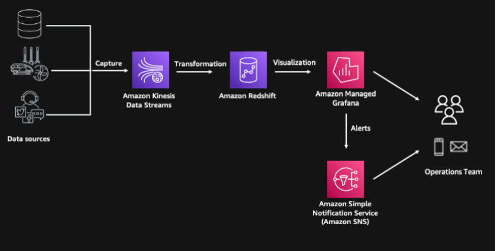
Prerequisites
The project has the following prerequisites:
- An AWS account.
- Amazon Linux 2 with AWS CDK, Docker CLI, and Python3 installed. Alternatively, setting up an AWS Cloud9 environment will satisfy this requirement.
- To run this code, you need elevated privileges into the AWS account you are using.
Sample deployment using the AWS CDK
The AWS CDK is an open-source project that allows you to define your cloud infrastructure using familiar programming languages. It uses high-level constructs to represent AWS components to simplify the build process. In this post, we use Python to define the cloud infrastructure due to its familiarity to many data and analytics professionals.
Clone the GitHub repository and install the Python dependencies:
Next, bootstrap the AWS CDK. This sets up the resources required by the AWS CDK to deploy into the AWS account. This step is only required if you haven’t used the AWS CDK in the deployment account and Region.
Deploy all stacks:
The entire deployment time takes 10–15 minutes.
Access streaming data using Amazon Redshift streaming ingestion
The AWS CDK deployment provisions an Amazon Redshift cluster with the appropriate default IAM role to access the Kinesis data stream. We can create an external schema to establish a connection between the Amazon Redshift cluster and the Kinesis data stream:
For instructions on how to connect to the cluster, refer to Connecting to the Redshift Cluster.
We use a materialized view to parse data in the Kinesis data stream. In this case, the whole payload is ingested as is and stored using the SUPER data type in Amazon Redshift. Data stored in streaming engines is usually in semi-structured format, and the SUPER data type provides a fast and efficient way to analyze semi-structured data within Amazon Redshift.

See the following code:
Refreshing the materialized view invokes Amazon Redshift to read data directly from the Kinesis data stream and load it into the materialized view. This refresh can be done automatically by adding the AUTO REFRESH clause in the materialized view definition. However, in this example, we are orchestrating the end-to-end data pipeline using AWS Step Functions.
Now we can start running queries against our streaming data and unify it with other datasets like logistics fleet data. If we want to know the distribution of our consignments across different states, we can easily unpack the contents of the JSON payload using the PartiQL syntax.
Generate features using Amazon Redshift SQL functions
The next step is to transform and enrich the streaming data using Amazon Redshift SQL to generate additional features that will be used by Amazon Redshift ML for its predictions. We use date and time functions to identify the day of the week, and calculate the number of days between the order date and target delivery date.
We also use geospatial functions, specifically ST\_DistanceSphere, to calculate the distance between origin and destination locations. The GEOMETRY data type within Amazon Redshift provides a cost-effective way to analyze geospatial data such as longitude and latitudes at scale. In this example, the addresses have already been converted to longitude and latitude. However, if you need to perform geocoding, you can integrate Amazon Location Services with Amazon Redshift using user-defined functions (UDFs). On top of geocoding, Amazon Location Service also allows you to more accurately calculate route distance between origin and destination, and even specify waypoints along the way.
We use another materialized view to persist these transformations. A materialized view provides a simple yet efficient way to create data pipelines using its incremental refresh capability. Amazon Redshift identifies the incremental changes from the last refresh and only updates the target materialized view based on these changes. In this materialized view, all our transformations are deterministic, so we expect our data to be consistent when going through a full refresh or an incremental refresh.

See the following code:
Predict delays using Amazon Redshift ML
We can use this enriched data to make predictions on the delay probability of a consignment. Amazon Redshift ML is a feature of Amazon Redshift that allows you to use the power of Amazon Redshift to build, train, and deploy ML models directly within your data warehouse.
The training of a new Amazon Redshift ML model has been initiated as part of the AWS CDK deployment using the CREATE MODEL statement. The training dataset is defined in the FROM clause, and TARGET defines which column the model is trying to predict. The FUNCTION clause defines the name of the function that is used to make predictions.
This simplified model is trained using historical observations, and the training process takes around 30 minutes to complete. You can check the status of the training job by running the SHOW MODEL statement:
When the model is ready, we can start making predictions on new data that is streamed into Amazon Redshift. Predictions are generated using the Amazon Redshift ML function that was defined during the training process. We pass the calculated features from the transformed materialized view into this function, and the prediction results populate the delay\_probability column.
This final output is persisted into the consignment\_predictions table, and Step Functions is orchestrating the ongoing incremental data load into this target table. We use a table for the final output, instead of a materialized view, because ML predictions have randomness involved and it may give us non-deterministic results. Using a table gives us more control on how data is loaded.

See the following code:
Create an Amazon Managed Grafana dashboard
We use Amazon Managed Grafana to create a near real-time logistics dashboard. Amazon Managed Grafana is a fully managed service that makes it easy to create, configure, and share interactive dashboards and charts for monitoring your data. We can also use Grafana to set up alerts and notifications based on specific conditions or thresholds, allowing you to quickly identify and respond to issues.
The high-level steps in setting up the dashboard are as follows:
- Create a Grafana workspace.
- Set up Grafana authentication using AWS IAM Identity Center (successor to AWS Single Sign-On) or using direct SAML integration.
- Configure Amazon Redshift as a Grafana data source.
- Import the JSON file for the near real-time logistics dashboard.
A more detailed set of instructions is available in the GitHub repository for your reference.
Clean up
To avoid ongoing charges, delete the resources deployed. Access the Amazon Linux 2 environment and run the AWS CDK destroy command. Delete the Grafana objects related to this deployment.
Conclusion
In this post, we showed how easy it is to build a near real-time logistics dashboard using Amazon Redshift and Amazon Managed Grafana. We created an end-to-end modern data pipeline using only SQL. This shows how Amazon Redshift is a powerful platform for democratizing your data—it enables a wide range of users, including business analysts, data scientists, and others, to work with and analyze data without requiring specialized technical skills or expertise.
We encourage you to explore what else can be achieved with Amazon Redshift and Amazon Managed Grafana. We also recommend you visit the AWS Big Data Blog for other useful blog posts on Amazon Redshift.
About the Author
 Paul Villena is an Analytics Solutions Architect in AWS with expertise in building modern data and analytics solutions to drive business value. He works with customers to help them harness the power of the cloud. His areas of interests are infrastructure-as-code, serverless technologies and coding in Python.
Apache Iceberg is an open table format for large datasets in Amazon Simple Storage Service (Amazon S3), and provides fast query performance over large tables, atomic commits, concurrent writes, and SQL-compatible table evolution. With Amazon EMR 6.5+, you can use Apache Spark on EMR clusters with the Iceberg table format.
Iceberg helps data engineers manage complex challenges such as continuously evolving datasets while maintaining query performance. Iceberg allows you to do the following:
- Maintain transactional consistency on tables between multiple applications where files can be added, removed, or modified atomically with full read isolation and multiple concurrent writes
- Implement full schema evolution to track changes to a table over time
- Issue time travel queries to query historical data and verify changes between updates
- Organize tables into flexible partition layouts with partition evolution, enabling updates to partition schemes as queries and data volume changes without relying on physical directories
- Roll back tables to prior versions to quickly correct issues and return tables to a known good state
- Perform advanced planning and filtering in high-performance queries on large datasets
In this post, we show you how to improve the performance of Iceberg’s metadata file operations using Amazon FSx for Lustre and Amazon EMR.
Performance of metadata file operations in Iceberg
The catalog, metadata layer, and data layer of Iceberg are outlined in the following diagram.

Iceberg maintains metadata across multiple small files (metadata file, manifest list, and manifest files) to effectively prune data, filter data, read the correct snapshot, merge delta files, and more. Although Iceberg has implemented fast scan planning to make sure that metadata file operations don’t take a large amount of time, the time taken is slightly high for object storage like Amazon S3 because it has a higher read/write latency.
In use cases like a high-throughput streaming application writing data into an S3 data lake in near-real time, snapshots are produced in microbatches at a very fast rate, resulting in a high number of snapshot files and causing degradation in performance of metadata file operations.
As shown in the following architecture diagram, the EMR cluster consumes from Kafka and writes to an Iceberg table, which uses Amazon S3 as storage and AWS Glue as the catalog.

In this post, we dive deep into how to improve query performance by caching metadata files in a low-latency file system like FSx for Lustre.
Overview of solution
FSx for Lustre makes it easy and cost-effective to launch and run the high-performance Lustre file system. You use it for workloads where speed matters, such as high throughput streaming writes, machine learning, high performance computing (HPC), video processing, and financial modelling. You can also link the FSx for Lustre file system to an S3 bucket, if required. FSx for Lustre offers multiple deployment options, including the following:
- Scratch file systems, which are designed for temporary storage and short-term processing of data. Data isn’t replicated and doesn’t persist if a file server fails. Use scratch file systems when you need cost-optimized storage for short-term, processing-heavy workloads.
- Persistent file systems, which are designed for long-term storage and workloads. The file servers are highly available, and data is automatically replicated within the same Availability Zone in which the file system is located. The data volumes attached to the file servers are replicated independently from the file servers to which they are attached.
The use case with Iceberg’s metadata files is related to caching, and the workloads are short-running (a few hours), so the scratch file system can be considered as a viable deployment option. A Scratch-2 file system with 200 MB/s/TiB of throughput is sufficient for our needs because Iceberg’s metadata files are small in size and we don’t expect a very high number of parallel connections.
You can use FSx for Lustre as a cache for the metadata files (on top of an S3 location) to offer better performance in terms of metadata file operations. To read/write files, Iceberg provides a capability to load a custom FileIO dynamically during runtime. You can pass the FSxForLustreS3FileIO reference using a Spark configuration, which takes care of reading/writing to appropriate file systems (FSx for Lustre for reads and Amazon S3 for writes). By enabling the catalog properties lustre.mount.path, lustre.file.system.path, and data.repository.path, Iceberg resolves the S3 path to FSx for Lustre path at runtime.
As shown in the following architecture diagram, the EMR cluster consumes from Kafka and writes to an Iceberg table that uses Amazon S3 as storage and AWS Glue as the catalog. Metadata reads are redirected to FSx for Lustre, which updates asynchronously.

Pricing and performance
We took a sample dataset across 100, 1,000, and 10,000 snapshots, and could observe up to 8.78 times speedup in metadata file operations and up to 1.26 times speedup in query time. Note that the benefit was observed for tables with a higher number of snapshots. The environment components used in this benchmark are listed in the following table.
| Iceberg Version | Spark Version | Cluster Version | Master | Workers |
| 0.14.1-amzn-0 | 3.3.0-amzn-1 | Amazon EMR 6.9.0 | m5.8xlarge | 15 x m5.8xlarge |
The following graph compares the speedup for each amount of snapshots.

You can calculate the price using the AWS Pricing Calculator. The estimated monthly cost of an FSx for Lustre file system (scratch deployment type) in the US East (N. Virginia) Region with 1.2 TB storage capacity and 200 MBps/TiB per unit storage throughput is $336.38.
The overall benefit is significant considering the low cost incurred. The performance gain in terms of metadata file operations can help you achieve low-latency read for high-throughput streaming workloads.
Prerequisites
For this walkthrough, you need the following prerequisites:
- An AWS account
- An Amazon Elastic Compute Cloud (Amazon EC2) key pair
- A VPC
Create an FSx for Lustre file system
In this section, we walk through the steps to create your FSx for Lustre file system via the FSx for Lustre console. To use the AWS Command Line Interface (AWS CLI), refer to create-file-system.
- On the Amazon FSx console, create a new file system.
- For File system options, select Amazon FSx for Lustre.
- Choose Next.

- For File system name¸ enter an optional name.
- For Deployment and storage type, select Scratch, SSD, because it’s designed for short-term storage and workloads.
- For Throughput per unit of storage, select 200 MB/s/TiB.You can choose the storage capacity according to your use case. A Scratch-2 file system with 200 MB/s/TiB of throughput is sufficient for our needs because Iceberg’s metadata files are small in size and we don’t expect a very high number of parallel connections.

- Enter an appropriate VPC, security group, and subnet.Make sure that the security group has the appropriate inbound and outbound rules enabled to access the FSx for Lustre file system from Amazon EMR.

- In the Data Repository Import/Export section, select Import data from and export data to S3.
- Select Update my file and directory listing as objects are added to, changed in, or deleted from my S3 bucket to keep the file system listing updated.
- For Import bucket, enter the S3 bucket to store the Iceberg metadata.

- Choose Next and verify the summary of the file system, then choose Create File System.
When the file system is created, you can view the DNS name and mount name.
Create an EMR cluster with FSx for Lustre mounted
This section shows how to create an Iceberg table using Spark, though we can use other engines as well. To create your EMR cluster with FSx for Lustre mounted, complete the following steps:
- On the Amazon EMR console, create an EMR cluster (6.9.0 or above) with Iceberg installed. For instructions, refer to Use a cluster with Iceberg installed.
To use the AWS CLI, refer to create-cluster.
- Keep the network (VPC) and EC2 subnet the same as the ones you used when creating the FSx for Lustre file system.

- Create a bootstrap script and upload it to an S3 bucket that is accessible to EMR.Refer to the following bootstrap script to mount FSx for Lustre in an EMR cluster (the file system gets mounted in the
/mnt/fsxpath of the cluster). The file system DNS name and the mount name can be found in the file system summary details. - Add the bootstrap action script to the EMR cluster.

- Specify your EC2 key pair.
- Choose Create cluster.

- When the EMR cluster is running, SSH into the cluster and launch the
spark-sqlusing the following code:
Note the following:
-
- At a Spark session level, the catalog properties
io-impl,lustre.mount.path,lustre.file.system.path, anddata.repository.pathhave been set. io-implsets a custom FileIO implementation that resolves the FSx for Lustre location (from the S3 location) during reads.lustre.mount.pathis the local mount path in the EMR cluster,lustre.file.system.pathis the FSx for Lustre file system path, anddata.repository.pathis the S3 data repository path, which is linked to the FSx for Lustre file system path. After all these properties are provided, thedata.repository.pathis resolved to the concatenation oflustre.mount.pathandlustre.file.system.pathduring reads. Note that FSx for Lustre is eventually consistent after an update in Amazon S3. So, in case FSx for Lustre is catching up with the S3 updates, theFileIOwill fall back to appropriate S3 paths.- If
write.metadata.pathis configured, make sure that the path doesn’t contain any trailing slashes anddata.repository.pathis equivalent towrite.metadata.path.
- At a Spark session level, the catalog properties
- Create the Iceberg database and table using the following queries:
Note that to migrate an existing table to use FSx for Lustre, you must create the FSx for Lustre file system, mount the same while starting the EMR cluster, and start the Spark session as highlighted in the previous step. The Amazon S3 listing of the existing table is updated in the FSx for Lustre file system eventually.
- Insert the data into the table using an
INSERT INTOquery and then query the same: - You can now view the metadata files in the local FSx mount, which is also linked to the S3 bucket
s3://<bucket>/warehouse/sample\_table/metadata/: - You can view the metadata files in Amazon S3:
- You can also view the data files in Amazon S3:
Clean up
When you’re done exploring the solution, complete the following steps to clean up the resources:
- Drop the Iceberg table.
- Delete the EMR cluster.
- Delete the FSx for Lustre file system.
- If any orphan files are present, empty the S3 bucket.
- Delete the EC2 key pair.
- Delete the VPC.
Conclusion
In this post, we demonstrated how to create an FSx for Lustre file system and an EMR cluster with the file system mounted. We observed the performance gain in terms of Iceberg metadata file operations and then cleaned up so as not to incur any additional charges.
Using FSx for Lustre with Iceberg on Amazon EMR allows you to gain significant performance in terms of metadata file operations. We observed 6.33–8.78 times speedup in metadata file operations and 1.06–1.26 times speedup in query time for Iceberg tables with 100, 1,000, and 10,000 snapshots. Note that this approach reduces the time for metadata file operations and not for the data operations. The overall performance gain would be dependent on the number of metadata files, size of each metadata files, amount of data that is being processed, and so on.
About the Author
 Rajarshi Sarkar is a Software Development Engineer at Amazon EMR. He works on cutting-edge features of Amazon EMR and is also involved in open-source projects such as Apache Iceberg and Trino. In his spare time, he likes to travel, watch movies and hang out with friends.
AWS re:Invent is a learning conference hosted by AWS for the global cloud computing community. Re:Invent was held at the end of 2022 in Las Vegas, Nevada, from November 28 to December 2.
Amazon QuickSight powers data-driven organizations with unified business intelligence (BI) at hyperscale. This post walks you through a full recap of QuickSight at this year’s re:Invent, including key launch announcements, sessions available virtually, and additional resources for continued learning.

Launch announcements
AWS Announces Five New Capabilities for Amazon QuickSight
This press release covers five new QuickSight capabilities to help you streamline business intelligence operations, using the most popular serverless BI service built for the cloud.
New analytical questions available in Amazon QuickSight Q: “Why” and “Forecast”
QuickSight announces support for two new question types that simplify and scale complex analytical tasks using natural language: “forecast” and “why.”
Announcing Automated Data Preparation for Amazon QuickSight Q
Automated data preparation utilizes machine learning (ML) to infer semantic information about data and adds it to datasets as metadata about the columns (fields), making it faster for you to prepare data in order to support natural language questions.
New Amazon QuickSight API Capabilities to Accelerate Your BI Transformation
New QuickSight API capabilities allow programmatic creation and management of dashboards, analysis, and templates.
Create and Share Operational Reports at Scale with Amazon QuickSight Paginated Reports
This feature allows you to create and share highly formatted, personalized reports containing business-critical data to hundreds of thousands of end-users—without any infrastructure setup or maintenance, up-front licensing, or long-term commitments.
Keynotes
Adam Selipsky, Chief Executive Officer of Amazon Web Services
Watch Adam Selipsky, Chief Executive Officer of Amazon Web Services, as he looks at the ways that forward-thinking builders are transforming industries and even our future, powered by AWS. He highlights innovations in data, infrastructure, and more that are helping customers achieve their goals faster, take advantage of untapped potential, and create a better future with AWS.
Swami Sivasubramanian, Vice President of AWS Data and Machine Learning
Watch Swami Sivasubramanian, Vice President of AWS Data and Machine Learning, as he reveals the latest AWS innovations that can help you transform your company’s data into meaningful insights and actions for your business. In this keynote, several speakers discuss the key components of a future-proof data strategy and how to empower your organization to drive the next wave of modern invention with data. Hear from leading AWS customers who are using data to bring new experiences to life for their customers.
Leadership sessions
Unlock the value of your data with AWS analytics
Data fuels digital transformation and drives effective business decisions. To survive in an ever-changing world, organizations are turning to data to derive insights, create new experiences, and reinvent themselves so they can remain relevant today and in the future. AWS offers analytics services that allow organizations to gain faster and deeper insights from all their data. In this session, G2 Krishnamoorthy, VP of AWS Analytics, addresses the current state of analytics on AWS, covers the latest service innovations around data, and highlights customer successes with AWS analytics. Also, learn from organizations like FINRA and more who have turned to AWS for their digital transformation journey.
Reinvent how you derive value from your data with Amazon QuickSight
In this session, learn how you can use AWS-native business analytics to provide your users with ML-powered interactive dashboards, natural language query (NLQ), and embedded analytics to provide insights to users at scale, when and where they need it. Watch this session to also learn more about how Amazon uses QuickSight internally.
Breakout sessions
What’s New with Amazon QuickSight?
This session covers all of QuickSight’s newly launched capabilities, including paginated reporting in the cloud, 1 billion rows of data with SPICE, assets as code, and new Amazon QuickSight Q capabilities, including ML-powered semantic inferencing, forecasting, new question types, and more.
Differentiate your apps with Amazon QuickSight embedded analytics
Watch this session to learn how to enable new monetization opportunities and grow your business with QuickSight embedded analytics. Discover how you can differentiate your end-user experience by embedding data visualizations, dashboards, and ML-powered natural language query into your applications at scale with no infrastructure to manage. Hear from customers Guardian Life and Showpad and learn more about their QuickSight use cases.
Migrate to cloud-native business analytics with Amazon QuickSight
Legacy BI systems can hurt agile decision-making in the modern organization, with expensive licensing, outdated capabilities, and expensive infrastructure management. In this session, discover how migrating your BI to the cloud with cloud-native, fully managed business analytics capabilities from QuickSight can help you overcome these challenges. Learn how you can use QuickSight’s interactive dashboards and reporting capabilities to provide insights to every user in the organization, lowering your costs and enabling better decision-making. Watch this session to also learn more about Siemens’s QuickSight use case.
Get clarity on your data in seconds with Amazon QuickSight Q
Amazon QuickSight Q is an ML–powered natural language capability that empowers business users to ask questions about all of their data using everyday business language and get answers in seconds. Q interprets questions to understand their intent and generates an answer instantly in the form of a visual without requiring authors to create graphics, dashboards, or analyses. In this session, the QuickSight Q team provides an overview and demonstration of Q in action. Watch this session to also learn more about NASDAQ’s QuickSight use case.
Optimize your AWS cost and usage with Cloud Intelligence Dashboards
Do your engineers know how much they’re spending? Do you have insight into the details of your cost and usage on AWS? Are you taking advantage of all your cost optimization opportunities? Attend this session to learn how organizations are using the Cloud Intelligence Dashboards to start their FinOps journeys and create cost-aware cultures within their organizations. Dive deep into specific use cases and learn how you can use these insights to drive and measure your cost optimization efforts. Discover how unit economics, resource-level visibility, and periodic spend updates make it possible for FinOps practitioners, developers, and business executives to come together to make smarter decisions. Watch this session to also learn more about Dolby laboratories’ QuickSight use case.
Useful resources
- QuickSight Community – Ask, answer, and learn with others in the QuickSight Community.
- QuickSight YouTube Channel – Subscribe to stay up to date on the latest QuickSight workshops, getting started tutorials, and demo videos.
- QuickSight DemoCentral – Experience QuickSight first-hand through interactive dashboards and demos.
- QuickSight workshops – Enhance your BI skills with self-paced QuickSight workshops.
With the QuickSight re:Invent breakout session recordings and additional resources, we hope that you learn how to dive deeper into your data with QuickSight. For continued learning, check out more information and resources via our website.
About the author
 Mia Heard is a product marketing manager for Amazon QuickSight, AWS’ cloud-native, fully managed BI service.
This is a guest post co-authored by Mahesh Vandi Chalil, Chief Technology Officer of BookMyShow.
BookMyShow (BMS), a leading entertainment company in India, provides an online ticketing platform for movies, plays, concerts, and sporting events. Selling up to 200 million tickets on an annual run rate basis (pre-COVID) to customers in India, Sri Lanka, Singapore, Indonesia, and the Middle East, BookMyShow also offers an online media streaming service and end-to-end management for virtual and on-ground entertainment experiences across all genres.
The pandemic gave BMS the opportunity to migrate and modernize our 15-year-old analytics solution to a modern data architecture on AWS. This architecture is modern, secure, governed, and cost-optimized architecture, with the ability to scale to petabytes. BMS migrated and modernized from on-premises and other cloud platforms to AWS in just four months. This project was run in parallel with our application migration project and achieved 90% cost savings in storage and 80% cost savings in analytics spend.
The BMS analytics platform caters to business needs for sales and marketing, finance, and business partners (e.g., cinemas and event owners), and provides application functionality for audience, personalization, pricing, and data science teams. The prior analytics solution had multiple copies of data, for a total of over 40 TB, with approximately 80 TB of data in other cloud storage. Data was stored on‑premises and in the cloud in various data stores. Growing organically, the teams had the freedom to choose their technology stack for individual projects, which led to the proliferation of various tools, technology, and practices. Individual teams for personalization, audience, data engineering, data science, and analytics used a variety of products for ingestion, data processing, and visualization.
This post discusses BMS’s migration and modernization journey, and how BMS, AWS, and AWS Partner Minfy Technologies team worked together to successfully complete the migration in four months and saving costs. The migration tenets using the AWS modern data architecture made the project a huge success.
Challenges in the prior analytics platform
- Varied Technology: Multiple teams used various products, languages, and versions of software.
- Larger Migration Project: Because the analytics modernization was a parallel project with application migration, planning was crucial in order to consider the changes in core applications and project timelines.
- Resources: Experienced resource churn from the application migration project, and had very little documentation of current systems.
- Data : Had multiple copies of data and no single source of truth; each data store provided a view for the business unit.
- Ingestion Pipelines: Complex data pipelines moved data across various data stores at varied frequencies. We had multiple approaches in place to ingest data to Cloudera, via over 100 Kafka consumers from transaction systems and MQTT(Message Queue Telemetry Transport messaging protocol) for clickstreams, stored procedures, and Spark jobs. We had approximately 100 jobs for data ingestion across Spark, Alteryx, Beam, NiFi, and more.
- Hadoop Clusters: Large dedicated hardware on which the Hadoop clusters were configured incurring fixed costs. On-premises Cloudera setup catered to most of the data engineering, audience, and personalization batch processing workloads. Teams had their implementation of HBase and Hive for our audience and personalization applications.
- Data warehouse: The data engineering team used TiDB as their on-premises data warehouse. However, each consumer team had their own perspective of data needed for analysis. As this siloed architecture evolved, it resulted in expensive storage and operational costs to maintain these separate environments.
- Analytics Database: The analytics team used data sourced from other transactional systems and denormalized data. The team had their own extract, transform, and load (ETL) pipeline, using Alteryx with a visualization tool.
Migration tenets followed which led to project success:
- Prioritize by business functionality.
- Apply best practices when building a modern data architecture from Day 1.
- Move only required data, canonicalize the data, and store it in the most optimal format in the target. Remove data redundancy as much possible. Mark scope for optimization for the future when changes are intrusive.
- Build the data architecture while keeping data formats, volumes, governance, and security in mind.
- Simplify ELT and processing jobs by categorizing the jobs as rehosted, rewritten, and retired. Finalize canonical data format, transformation, enrichment, compression, and storage format as Parquet.
- Rehost machine learning (ML) jobs that were critical for business.
- Work backward to achieve our goals, and clear roadblocks and alter decisions to move forward.
- Use serverless options as a first option and pay per use. Assess the cost and effort for rearchitecting to select the right approach. Execute a proof of concept to validate this for each component and service.
Strategies applied to succeed in this migration:
- Team – We created a unified team with people from data engineering, analytics, and data science as part of the analytics migration project. Site reliability engineering (SRE) and application teams were involved when critical decisions were needed regarding data or timeline for alignment. The analytics, data engineering, and data science teams spent considerable time planning, understanding the code, and iteratively looking at the existing data sources, data pipelines, and processing jobs. AWS team with partner team from Minfy Technologies helped BMS arrive at a migration plan after a proof of concept for each of the components in data ingestion, data processing, data warehouse, ML, and analytics dashboards.
- Workshops – The AWS team conducted a series of workshops and immersion days, and coached the BMS team on the technology and best practices to deploy the analytics services. The AWS team helped BMS explore the configuration and benefits of the migration approach for each scenario (data migration, data pipeline, data processing, visualization, and machine learning) via proof-of-concepts (POCs). The team captured the changes required in the existing code for migration. BMS team also got acquainted with the following AWS services:
- Proof of concept – The BMS team, with help from the partner and AWS team, implemented multiple proofs of concept to validate the migration approach:
- Performed batch processing of Spark jobs in Amazon EMR, in which we checked the runtime, required code changes, and cost.
- Ran clickstream analysis jobs in Amazon EMR, testing the end-to-end pipeline. Team conducted proofs of concept on AWS IoT Core for MQTT protocol and streaming to Amazon S3.
- Migrated ML models to Amazon SageMaker and orchestrated with Amazon MWAA.
- Created sample QuickSight reports and dashboards, in which features and time to build were assessed.
- Configured for key scenarios for Amazon Redshift, in which time for loading data, query performance, and cost were assessed.
- Effort vs. cost analysis – Team performed the following assessments:
- Compared the ingestion pipelines, the difference in data structure in each store, the basis of the current business need for the data source, the activity for preprocessing the data before migration, data migration to Amazon S3, and change data capture (CDC) from the migrated applications in AWS.
- Assessed the effort to migrate approximately 200 jobs, determined which jobs were redundant or need improvement from a functional perspective, and completed a migration list for the target state. The modernization of the MQTT workflow code to serverless was time-consuming, decided to rehost on Amazon Elastic Compute Cloud (Amazon EC2) and modernization to Amazon Kinesis in to the next phase.
- Reviewed over 400 reports and dashboards, prioritized development in phases, and reassessed business user needs.
AWS cloud services chosen for proposed architecture:
- Data lake – We used Amazon S3 as the data lake to store the single truth of information for all raw and processed data, thereby reducing the copies of data storage and storage costs.
- Ingestion – Because we had multiple sources of truth in the current architecture, we arrived at a common structure before migration to Amazon S3, and existing pipelines were modified to do preprocessing. These one-time preprocessing jobs were run in Cloudera, because the source data was on-premises, and on Amazon EMR for data in the cloud. We designed new data pipelines for ingestion from transactional systems on the AWS cloud using AWS Glue ETL.
- Processing – Processing jobs were segregated based on runtime into two categories: batch and near-real time. Batch processes were further divided into transient Amazon EMR clusters with varying runtimes and Hadoop application requirements like HBase. Near-real-time jobs were provisioned in an Amazon EMR permanent cluster for clickstream analytics, and a data pipeline from transactional systems. We adopted a serverless approach using AWS Glue ETL for new data pipelines from transactional systems on the AWS cloud.
- Data warehouse – We chose Amazon Redshift as our data warehouse, and planned on how the data would be distributed based on query patterns.
- Visualization – We built the reports in Amazon QuickSight in phases and prioritized them based on business demand. We discussed with business users their current needs and identified the immediate reports required. We defined the phases of report and dashboard creation and built the reports in Amazon QuickSight. We plan to use embedded reports for external users in the future.
- Machine learning – Custom ML models were deployed on Amazon SageMaker. Existing Airflow DAGs were migrated to Amazon MWAA.
- Governance, security, and compliance – Governance with Amazon Lake Formation was adopted from Day 1. We configured the AWS Glue Data Catalog to reference data used as sources and targets. We had to comply to Payment Card Industry (PCI) guidelines because payment information was in the data lake, so we ensured the necessary security policies.
Solution overview
BMS modern data architecture
The following diagram illustrates our modern data architecture.

The architecture includes the following components:
- Source systems – These include the following:
- Data from transactional systems stored in MariaDB (booking and transactions).
- User interaction clickstream data via Kafka consumers to DataOps MariaDB.
- Members and seat allocation information from MongoDB.
- SQL Server for specific offers and payment information.
- Data pipeline – Spark jobs on an Amazon EMR permanent cluster process the clickstream data from Kafka clusters.
- Data lake – Data from source systems was stored in their respective Amazon S3 buckets, with prefixes for optimized data querying. For Amazon S3, we followed a hierarchy to store raw, summarized, and team or service-related data in different parent folders as per the source and type of data. Lifecycle polices were added to logs and temp folders of different services as per teams’ requirements.
- Data processing – Transient Amazon EMR clusters are used for processing data into a curated format for the audience, personalization, and analytics teams. Small file merger jobs merge the clickstream data to a larger file size, which saved costs for one-time queries.
- Governance – AWS Lake Formation enables the usage of AWS Glue crawlers to capture the schema of data stored in the data lake and version changes in the schema. The Data Catalog and security policy in AWS Lake Formation enable access to data for roles and users in Amazon Redshift, Amazon Athena, Amazon QuickSight, and data science jobs. AWS Glue ETL jobs load the processed data to Amazon Redshift at scheduled intervals.
- Queries – The analytics team used Amazon Athena to perform one-time queries raised from business teams on the data lake. Because report development is in phases, Amazon Athena was used for exporting data.
- Data warehouse – Amazon Redshift was used as the data warehouse, where the reports for the sales teams, management, and third parties (i.e., theaters and events) are processed and stored for quick retrieval. Views to analyze the total sales, movie sale trends, member behavior, and payment modes are configured here. We use materialized views for denormalized tables, different schemas for metadata, and transactional and behavior data.
- Reports – We used Amazon QuickSight reports for various business, marketing, and product use cases.
- Machine learning – Some of the models deployed on Amazon SageMaker are as follows:
- Content popularity – Decides the recommended content for users.
- Live event popularity – Calculates the popularity of live entertainment events in different regions.
- Trending searches – Identifies trending searches across regions.
Walkthrough
Migration execution steps
We standardized tools, services, and processes for data engineering, analytics, and data science:
- Data lake
- Identified the source data to be migrated from Archival DB, BigQuery, TiDB, and the analytics database.
- Built a canonical data model that catered to multiple business teams and reduced the copies of data, and therefore storage and operational costs. Modified existing jobs to facilitate migration to a canonical format.
- Identified the source systems, capacity required, anticipated growth, owners, and access requirements.
- Ran the bulk data migration to Amazon S3 from various sources.
- Ingestion
- Transaction systems – Retained the existing Kafka queues and consumers.
- Clickstream data – Successfully conducted a proof of concept to use AWS IoT Core for MQTT protocol. But because we needed to make changes in the application to publish to AWS IoT Core, we decided to implement it as part of mobile application modernization at a later time. We decided to rehost the MQTT server on Amazon EC2.
- Processing
- Listed the data pipelines relevant to business and migrated them with minimal modification.
- Categorized workloads into critical jobs, redundant jobs, or jobs that can be optimized:
- Spark jobs were migrated to Amazon EMR.
- HBase jobs were migrated to Amazon EMR with HBase.
- Metadata stored in Hive-based jobs were modified to use the AWS Glue Data Catalog.
- NiFi jobs were simplified and rewritten in Spark run in Amazon EMR.
- Amazon EMR clusters were configured one persistent cluster for streaming the clickstream and personalization workloads. We used multiple transient clusters for running all other Spark ETL or processing jobs. We used Spot Instances for task nodes to save costs. We optimized data storage with specific jobs to merge small files and compressed file format conversions.
- AWS Glue crawlers identified new data in Amazon S3. AWS Glue ETL jobs transformed and uploaded processed data to the Amazon Redshift data warehouse.
- Datawarehouse
- Defined the data warehouse schema by categorizing the critical reports required by the business, keeping in mind the workload and reports required in future.
- Defined the staging area for incremental data loaded into Amazon Redshift, materialized views, and tuning the queries based on usage. The transaction and primary metadata are stored in Amazon Redshift to cater to all data analysis and reporting requirements. We created materialized views and denormalized tables in Amazon Redshift to use as data sources for Amazon QuickSight dashboards and segmentation jobs, respectively.
- Optimally used the Amazon Redshift cluster by loading last two years data in Amazon Redshift, and used Amazon Redshift Spectrum to query historical data through external tables. This helped balance the usage and cost of the Amazon Redshift cluster.
- Visualization
- Amazon QuickSight dashboards were created for the sales and marketing team in Phase 1:
- Sales summary report – An executive summary dashboard to get an overview of sales across the country by region, city, movie, theatre, genre, and more.
- Live entertainment – A dedicated report for live entertainment vertical events.
- Coupons – A report for coupons purchased and redeemed.
- BookASmile – A dashboard to analyze the data for BookASmile, a charity initiative.
- Amazon QuickSight dashboards were created for the sales and marketing team in Phase 1:
- Machine learning
- Listed the ML workloads to be migrated based on current business needs.
- Priority ML processing jobs were deployed on Amazon EMR. Models were modified to use Amazon S3 as source and target, and new APIs were exposed to use the functionality. ML models were deployed on Amazon SageMaker for movies, live event clickstream analysis, and personalization.
- Existing artifacts in Airflow orchestration were migrated to Amazon MWAA.
- Security
- AWS Lake Formation was the foundation of the data lake, with the AWS Glue Data Catalog as the foundation for the central catalog for the data stored in Amazon S3. This provided access to the data by various functionalities, including the audience, personalization, analytics, and data science teams.
- Personally identifiable information (PII) and payment data was stored in the data lake and data warehouse, so we had to comply to PCI guidelines. Encryption of data at rest and in transit was considered and configured in each service level (Amazon S3, AWS Glue Data Catalog, Amazon EMR, AWS Glue, Amazon Redshift, and QuickSight). Clear roles, responsibilities, and access permissions for different user groups and privileges were listed and configured in AWS Identity and Access Management (IAM) and individual services.
- Existing single sign-on (SSO) integration with Microsoft Active Directory was used for Amazon QuickSight user access.
- Automation
- We used AWS CloudFormation for the creation and modification of all the core and analytics services.
- AWS Step Functions was used to orchestrate Spark jobs on Amazon EMR.
- Scheduled jobs were configured in AWS Glue for uploading data in Amazon Redshift based on business needs.
- Monitoring of the analytics services was done using Amazon CloudWatch metrics, and right-sizing of instances and configuration was achieved. Spark job performance on Amazon EMR was analyzed using the native Spark logs and Spark user interface (UI).
- Lifecycle policies were applied to the data lake to optimize the data storage costs over time.
Benefits of a modern data architecture
A modern data architecture offered us the following benefits:
- Scalability – We moved from a fixed infrastructure to the minimal infrastructure required, with configuration to scale on demand. Services like Amazon EMR and Amazon Redshift enable us to do this with just a few clicks.
- Agility – We use purpose-built managed services instead of reinventing the wheel. Automation and monitoring were key considerations, which enable us to make changes quickly.
- Serverless – Adoption of serverless services like Amazon S3, AWS Glue, Amazon Athena, AWS Step Functions, and AWS Lambda support us when our business has sudden spikes with new movies or events launched.
- Cost savings – Our storage size was reduced by 90%. Our overall spend on analytics and ML was reduced by 80%.
Conclusion
In this post, we showed you how a modern data architecture on AWS helped BMS to easily share data across organizational boundaries. This allowed BMS to make decisions with speed and agility at scale; ensure compliance via unified data access, security, and governance; and to scale systems at a low cost without compromising performance. Working with the AWS and Minfy Technologies teams helped BMS choose the correct technology services and complete the migration in four months. BMS achieved the scalability and cost-optimization goals with this updated architecture, which has set the stage for innovation using graph databases and enhanced our ML projects to improve customer experience.
About the Authors
 Mahesh Vandi Chalil is Chief Technology Officer at BookMyShow, India’s leading entertainment destination. Mahesh has over two decades of global experience, passionate about building scalable products that delight customers while keeping innovation as the top goal motivating his team to constantly aspire for these. Mahesh invests his energies in creating and nurturing the next generation of technology leaders and entrepreneurs, both within the organization and outside of it. A proud husband and father of two daughters and plays cricket during his leisure time.
 Priya Jathar is a Solutions Architect working in Digital Native Business segment at AWS. She has more two decades of IT experience, with expertise in Application Development, Database, and Analytics. She is a builder who enjoys innovating with new technologies to achieve business goals. Currently helping customers Migrate, Modernise, and Innovate in Cloud. In her free time she likes to paint, and hone her gardening and cooking skills.
 Vatsal Shah is a Senior Solutions Architect at AWS based out of Mumbai, India. He has more than nine years of industry experience, including leadership roles in product engineering, SRE, and cloud architecture. He currently focuses on enabling large startups to streamline their cloud operations and help them scale on the cloud. He also specializes in AI and Machine Learning use cases.
Extract, Load, and Transform (ELT) is a modern design strategy where raw data is first loaded into the data warehouse and then transformed with familiar Structured Query Language (SQL) semantics leveraging the power of massively parallel processing (MPP) architecture of the data warehouse. When you use an ELT pattern, you can also use your existing SQL workload while migrating from your on-premises data warehouse to Amazon Redshift. This eliminates the need to rewrite relational and complex SQL workloads into a new framework. With Amazon Redshift, you can load, transform, and enrich your data efficiently using familiar SQL with advanced and robust SQL support, simplicity, and seamless integration with your existing SQL tools. When you adopt an ELT pattern, a fully automated and highly scalable workflow orchestration mechanism will help to minimize the operational effort that you must invest in managing the pipelines. It also ensures the timely and accurate refresh of your data warehouse.
AWS Step Functions is a low-code, serverless, visual workflow service where you can orchestrate complex business workflows with an event-driven framework and easily develop repeatable and dependent processes. It can ensure that the long-running, multiple ELT jobs run in a specified order and complete successfully instead of manually orchestrating those jobs or maintaining a separate application.
Amazon DynamoDB is a fast, flexible NoSQL database service for single-digit millisecond performance at any scale.
This post explains how to use AWS Step Functions, Amazon DynamoDB, and Amazon Redshift Data API to orchestrate the different steps in your ELT workflow and process data within the Amazon Redshift data warehouse.
Solution overview
In this solution, we will orchestrate an ELT process using AWS Step Functions. As part of the ELT process, we will refresh the dimension and fact tables at regular intervals from staging tables, which ingest data from the source. We will maintain the current state of the ELT process (e.g., Running or Ready) in an audit table that will be maintained at Amazon DynamoDB. AWS Step Functions allows you to directly call the Data API from a state machine, reducing the complexity of running the ELT pipeline. For loading the dimensions and fact tables, we will be using Amazon Redshift Data API from AWS Lambda. We will use Amazon EventBridge for scheduling the state machine to run at a desired interval based on the customer’s SLA.
For a given ELT process, we will set up a JobID in a DynamoDB audit table and set the JobState as “Ready” before the state machine runs for the first time. The state machine performs the following steps:
- The first process in the Step Functions workflow is to pass the
JobIDas input to the process that is configured asJobID101 in Step Functions and DynamoDB by default via the CloudFormation template. - The next step is to fetch the current
JobStatefor the givenJobIDby running a query against the DynamoDB audit table using Lambda Data API. - If
JobStateis “Running,” then it indicates that the previous iteration is not completed yet, and the process should end. - If the
JobStateis “Ready,” then it indicates that the previous iteration was completed successfully and the process is ready to start. So, the next step will be to update the DynamoDB audit table to change theJobStateto “Running” andJobStartto the current time for the givenJobIDusing DynamoDB Data API within a Lambda function. - The next step will be to start the dimension table load from the staging table data within Amazon Redshift using Lambda Data API. In order to achieve that, we can either call a stored procedure using the Amazon Redshift Data API, or we can also run series of SQL statements synchronously using Amazon Redshift Data API within a Lambda function.
- In a typical data warehouse, multiple dimension tables are loaded in parallel at the same time before the fact table gets loaded. Using Parallel flow in Step Functions, we will load two dimension tables at the same time using Amazon Redshift Data API within a Lambda function.
- Once the load is completed for both the dimension tables, we will load the fact table as the next step using Amazon Redshift Data API within a Lambda function.
- As the load completes successfully, the last step would be to update the DynamoDB audit table to change the
JobStateto “Ready” andJobEndto the current time for the givenJobID, using DynamoDB Data API within a Lambda function.
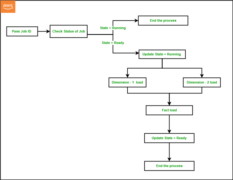
Components and dependencies
The following architecture diagram highlights the end-to-end solution using AWS services:

Before diving deeper into the code, let’s look at the components first:
- AWS Step Functions – You can orchestrate a workflow by creating a State Machine to manage failures, retries, parallelization, and service integrations.
- Amazon EventBridge – You can run your state machine on a daily schedule by creating a Rule in Amazon EventBridge.
- AWS Lambda – You can trigger a Lambda function to run Data API either from Amazon Redshift or DynamoDB.
- Amazon DynamoDB – Amazon DynamoDB is a fully managed, serverless, key-value NoSQL database designed to run high-performance applications at any scale. DynamoDB is extremely efficient in running updates, which improves the performance of metadata management for customers with strict SLAs.
- Amazon Redshift – Amazon Redshift is a fully managed, scalable cloud data warehouse that accelerates your time to insights with fast, easy, and secure analytics at scale.
- Amazon Redshift Data API – You can access your Amazon Redshift database using the built-in Amazon Redshift Data API. Using this API, you can access Amazon Redshift data with web services–based applications, including AWS Lambda.
- DynamoDB API – You can access your Amazon DynamoDB tables from a Lambda function by importing boto3.
Prerequisites
To complete this walkthrough, you must have the following prerequisites:
- An AWS account.
- An Amazon Redshift cluster.
- An Amazon Redshift customizable IAM service role with the following policies:
AmazonS3ReadOnlyAccessAmazonRedshiftFullAccess
- Above IAM role associated to the Amazon Redshift cluster.
Deploy the CloudFormation template
To set up the ETL orchestration demo, the steps are as follows:
- Sign in to the AWS Management Console.
- Click on Launch Stack.
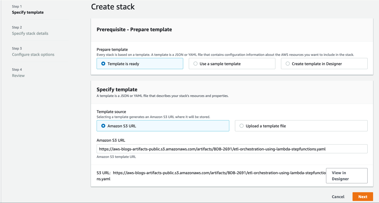
- Click Next.
- Enter a suitable name in Stack name.
- Provide the information for the Parameters as detailed in the following table.
| CloudFormation template parameter | Allowed values | Description |
RedshiftClusterIdentifier | Amazon Redshift cluster identifier | Enter the Amazon Redshift cluster identifier |
DatabaseUserName | Database user name in Amazon Redshift cluster | Amazon Redshift database user name which has access to run SQL Script |
DatabaseName | Amazon Redshift database name | Name of the Amazon Redshift primary database where SQL script would be run |
RedshiftIAMRoleARN | Valid IAM role ARN attached to Amazon Redshift cluster | AWS IAM role ARN associated with the Amazon Redshift cluster |

- Click Next and a new page appears. Accept the default values in the page and click Next. On the last page check the box to acknowledge resources might be created and click on Create stack.

- Monitor the progress of the stack creation and wait until it is complete.
- The stack creation should complete approximately within 5 minutes.
- Navigate to Amazon Redshift console.
- Launch Amazon Redshift query editor v2 and connect to your cluster.
- Browse to the database name provided in the parameters while creating the cloudformation template e.g., dev, public schema and expand Tables. You should see the tables as shown below.

- Validate the sample data by running the following SQL query and confirm the row count match above the screenshot.
Run the ELT orchestration
- After you deploy the CloudFormation template, navigate to the stack detail page. On the Resources tab, choose the link for DynamoDBETLAuditTable to be redirected to the DynamoDB console.
- Navigate to Tables and click on table name beginning with <stackname>-DynamoDBETLAuditTable. In this demo, the stack name is
DemoETLOrchestration, so the table name will begin withDemoETLOrchestration-DynamoDBETLAuditTable. - It will expand the table. Click on Explore table items.
- Here you can see the current status of the job, which will be in
Readystatus.

- Navigate again to stack detail page on the CloudFormation console. On the Resources tab, choose the link for RedshiftETLStepFunction to be redirected to the Step Functions console.
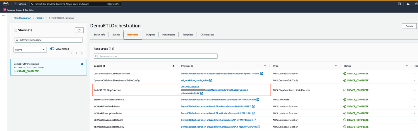
- Click Start Execution. When it successfully completes, all steps will be marked as green.

- While the job is running, navigate back to DemoETLOrchestration-DynamoDBETLAuditTable in the DynamoDB console screen. You will see JobState as
Runningwith JobStart time.
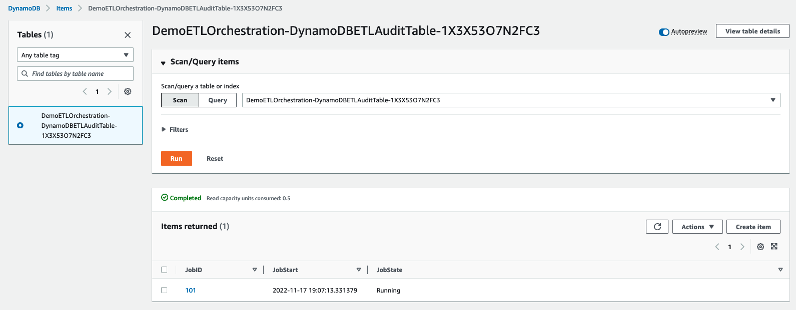
- After Step Functions completes, JobState will be changed to
Readywith JobStart and JobEnd time.
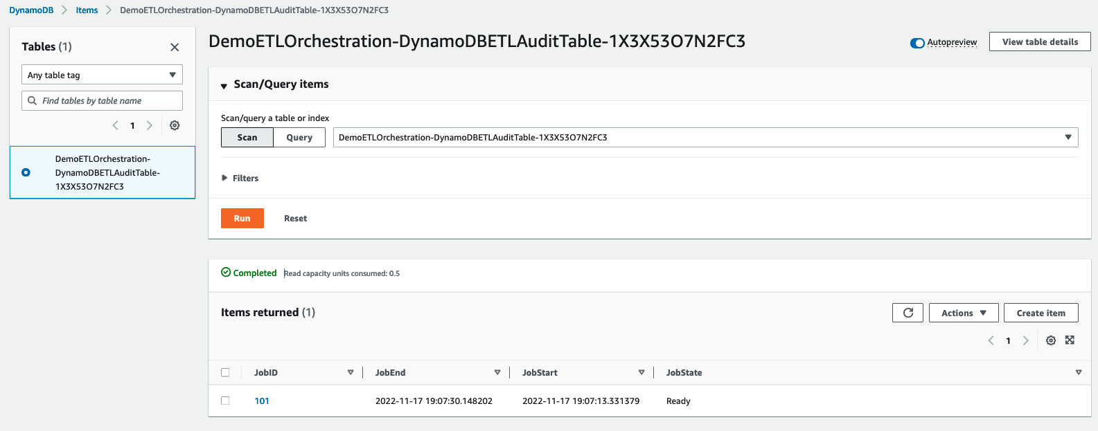
Handling failure
In the real world sometimes, the ELT process can fail due to unexpected data anomalies or object related issues. In that case, the step function execution will also fail with the failed step marked in red as shown in the screenshot below:

Once you identify and fix the issue, please follow the below steps to restart the step function:
- Navigate to the DynamoDB table beginning with
DemoETLOrchestration-DynamoDBETLAuditTable. Click on Explore table items and select the row with the specific JobID for the failed job. - Go to Action and select Edit item to modify the JobState to
Readyas shown below:

- Follow steps 5 and 6 under the “Run the ELT orchestration” section to restart execution of the step function.
Validate the ELT orchestration
The step function loads the dimension tables public.supplier and public.customer and the fact table public.fact\_yearly\_sale. To validate the orchestration, the process steps are as follows:
- Navigate to the Amazon Redshift console.
- Launch Amazon Redshift query editor v2 and connect to your cluster.
- Browse to the database name provided in the parameters while creating the cloud formation template e.g., dev, public schema.
- Validate the data loaded by Step Functions by running the following SQL query and confirm the row count to match as follows:
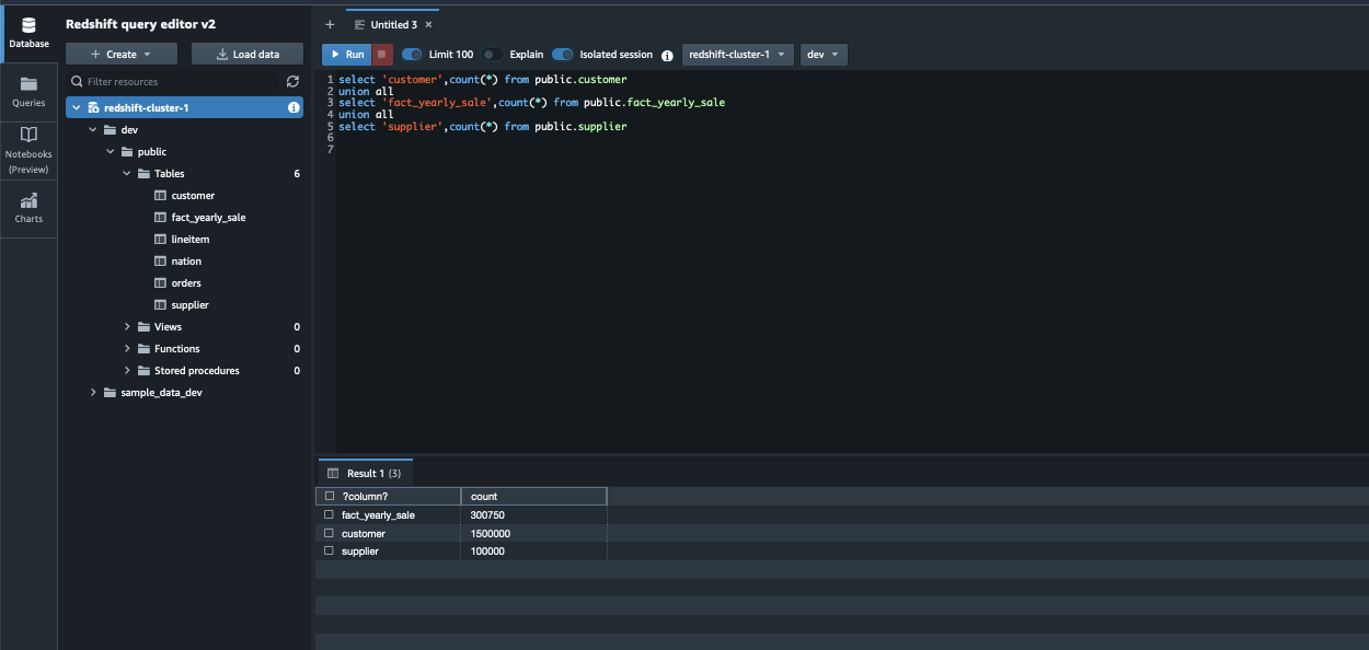
Schedule the ELT orchestration
The steps are as follows to schedule the Step Functions:
- Navigate to the Amazon EventBridge console and choose Create rule.
- Under Name, enter a meaningful name, for example,
Trigger-Redshift-ELTStepFunction. - Under Event bus, choose
default. - Under Rule Type, select
Schedule. - Click on Next.

- Under Schedule pattern, select
A schedule that runs at a regular rate, such as every 10 minutes. - Under Rate expression, enter Value as
5and choose Unit asMinutes. - Click on Next.

- Under Target types, choose
AWS service. - Under Select a Target, choose
Step Functions state machine. - Under State machine, choose the step function created by the CloudFormation template.
- Under Execution role, select
Create a new role for this specific resource. - Click on Next.

- Review the rule parameters and click on Create Rule.
After the rule has been created, it will automatically trigger the step function every 5 minutes to perform ELT processing in Amazon Redshift.
Clean up
Please note that deploying a CloudFormation template incurs cost. To avoid incurring future charges, delete the resources you created as part of the CloudFormation stack by navigating to the AWS CloudFormation console, selecting the stack, and choosing Delete.
Conclusion
In this post, we described how to easily implement a modern, serverless, highly scalable, and cost-effective ELT workflow orchestration process in Amazon Redshift using AWS Step Functions, Amazon DynamoDB and Amazon Redshift Data API. As an alternate solution, you can also use Amazon Redshift for metadata management instead of using Amazon DynamoDB. As part of this demo, we show how a single job entry in DynamoDB gets updated for each run, but you can also modify the solution to maintain a separate audit table with the history of each run for each job, which would help with debugging or historical tracking purposes. Step Functions manage failures, retries, parallelization, service integrations, and observability so your developers can focus on higher-value business logic. Step Functions can integrate with Amazon SNS to send notifications in case of failure or success of the workflow. Please follow this AWS Step Functions documentation to implement the notification mechanism.
About the Authors
 Poulomi Dasgupta is a Senior Analytics Solutions Architect with AWS. She is passionate about helping customers build cloud-based analytics solutions to solve their business problems. Outside of work, she likes travelling and spending time with her family.
Raks Khare is an Analytics Specialist Solutions Architect at AWS based out of Pennsylvania. He helps customers architect data analytics solutions at scale on the AWS platform.
Tahir Aziz is an Analytics Solution Architect at AWS. He has worked with building data warehouses and big data solutions for over 13 years. He loves to help customers design end-to-end analytics solutions on AWS. Outside of work, he enjoys traveling
and cooking.
Amazon EMR Serverless allows you to run open-source big data frameworks such as Apache Spark and Apache Hive without managing clusters and servers. Many customers who run Spark and Hive applications want to add their own libraries and dependencies to the application runtime. For example, you may want to add popular open-source extensions to Spark, or add a customized encryption-decryption module that is used by your application.
We are excited to announce a new capability that allows you to customize the runtime image used in EMR Serverless by adding custom libraries that your applications need to use. This feature enables you to do the following:
- Maintain a set of version-controlled libraries that are reused and available for use in all your EMR Serverless jobs as part of the EMR Serverless runtime
- Add popular extensions to open-source Spark and Hive frameworks such as pandas, NumPy, matplotlib, and more that you want your EMR serverless application to use
- Use established CI/CD processes to build, test, and deploy your customized extension libraries to the EMR Serverless runtime
- Apply established security processes, such as image scanning, to meet the compliance and governance requirements within your organization
- Use a different version of a runtime component (for example the JDK runtime or the Python SDK runtime) than the version that is available by default with EMR Serverless
In this post, we demonstrate how to use this new feature.
Solution Overview
To use this capability, customize the EMR Serverless base image using Amazon Elastic Container Registry (Amazon ECR), which is a fully managed container registry that makes it easy for your developers to share and deploy container images. Amazon ECR eliminates the need to operate your own container repositories or worry about scaling the underlying infrastructure. After the custom image is pushed to the container registry, specify the custom image while creating your EMR Serverless applications.
The following diagram illustrates the steps involved in using custom images for your EMR Serverless applications.

In the following sections, we demonstrate using custom images with Amazon EMR Serverless to address three common use cases:
- Add popular open-source Python libraries into the EMR Serverless runtime image
- Use a different or newer version of the Java runtime for the EMR Serverless application
- Install a Prometheus agent and customize the Spark runtime to push Spark JMX metrics to Amazon Managed Service for Prometheus, and visualize the metrics in a Grafana dashboard
General prerequisites
The following are the prerequisites to use custom images with EMR Serverless. Complete the following steps before proceeding with the subsequent steps:
- Create an AWS Identity and Access Management (IAM) role with IAM permissions for Amazon EMR Serverless applications, Amazon ECR permissions, and Amazon S3 permissions for the Amazon Simple Storage Service (Amazon S3) bucket
aws-bigdata-blogand any S3 bucket in your account where you will store the application artifacts. - Install or upgrade to the latest AWS Command Line Interface (AWS CLI) version and install the Docker service in an Amazon Linux 2 based Amazon Elastic Compute Cloud (Amazon EC2) instance. Attach the IAM role from the previous step for this EC2 instance.
- Select a base EMR Serverless image from the following public Amazon ECR repository. Run the following commands on the EC2 instance with Docker installed to verify that you are able to pull the base image from the public repository:
- Log in to Amazon ECR with the following commands and create a repository called
emr-serverless-ci-examples, providing your AWS account ID and Region: - Provide IAM permissions to the EMR Serverless service principal for the Amazon ECR repository:
- On the Amazon ECR console, choose Permissions under Repositories in the navigation pane.
- Choose Edit policy JSON.

- Enter the following JSON and save:
Make sure that the policy is updated on the Amazon ECR console.

For production workloads, we recommend adding a condition in the Amazon ECR policy to ensure only allowed EMR Serverless applications can get, describe, and download images from this repository. For more information, refer to Allow EMR Serverless to access the custom image repository.
In the next steps, we create and use custom images in our EMR Serverless applications for the three different use cases.
Use case 1: Run data science applications
One of the common applications of Spark on Amazon EMR is the ability to run data science and machine learning (ML) applications at scale. For large datasets, Spark includes SparkML, which offers common ML algorithms that can be used to train models in a distributed fashion. However, you often need to run many iterations of simple classifiers to fit for hyperparameter tuning, ensembles, and multi-class solutions over small-to-medium-sized data (100,000 to 1 million records). Spark is a great engine to run multiple iterations of such classifiers in parallel. In this example, we demonstrate this use case, where we use Spark to run multiple iterations of an XGBoost model to select the best parameters. The ability to include Python dependencies in the EMR Serverless image should make it easy to make the various dependencies (xgboost, sk-dist, pandas, numpy, and so on) available for the application.
Prerequisites
The EMR Serverless job runtime IAM role should be given permissions to your S3 bucket where you will be storing your PySpark file and application logs:
Create an image to install ML dependencies
We create a custom image from the base EMR Serverless image to install dependencies required by the SparkML application. Create the following Dockerfile in your EC2 instance that runs the docker process inside a new directory named datascience:
Build and push the image to the Amazon ECR repository emr-serverless-ci-examples, providing your AWS account ID and Region:
Submit your Spark application
Create an EMR Serverless application with the custom image created in the previous step:
Make a note of the value of applicationId returned by the command.
After the application is created, we’re ready to submit our job. Copy the application file to your S3 bucket:
Submit the Spark data science job. In the following command, provide the name of the S3 bucket and prefix where you stored your application file. Additionally, provide the applicationId value obtained from the create-application command and your EMR Serverless job runtime IAM role ARN.
After the Spark job succeeds, you can view the best model estimates from our application by viewing the Spark driver’s stdout logs. Navigate to Spark History Server, Executors, Driver, Logs, stdout.

Use case 2: Use a custom Java runtime environment
Another use case for custom images is the ability to use a custom Java version for your EMR Serverless applications. For example, if you’re using Java11 to compile and package your Java or Scala applications, and try to run them directly on EMR Serverless, it may lead to runtime errors because EMR Serverless uses Java 8 JRE by default. To make the runtime environments of your EMR Serverless applications compatible with your compile environment, you can use the custom images feature to install the Java version you are using to package your applications.
Prerequisites
An EMR Serverless job runtime IAM role should be given permissions to your S3 bucket where you will be storing your application JAR and logs:
Create an image to install a custom Java version
We first create an image that will install a Java 11 runtime environment. Create the following Dockerfile in your EC2 instance inside a new directory named customjre:
Build and push the image to the Amazon ECR repository emr-serverless-ci-examples, providing your AWS account ID and Region:
Submit your Spark application
Create an EMR Serverless application with the custom image created in the previous step:
Copy the application JAR to your S3 bucket:
Submit a Spark Scala job that was compiled with Java11 JRE. This job also uses Java APIs that may produce different results for different versions of Java (for example: java.time.ZoneId). In the following command, provide the name of the S3 bucket and prefix where you stored your application JAR. Additionally, provide the applicationId value obtained from the create-application command and your EMR Serverless job runtime role ARN with IAM permissions mentioned in the prerequisites. Note that in the sparkSubmitParameters, we pass a custom Java version for our Spark driver and executor environments to instruct our job to use the Java11 runtime.
You can also extend this use case to install and use a custom Python version for your PySpark applications.
Use case 3: Monitor Spark metrics in a single Grafana dashboard
Spark JMX telemetry provides a lot of fine-grained details about every stage of the Spark application, even at the JVM level. These insights can be used to tune and optimize the Spark applications to reduce job runtime and cost. Prometheus is a popular tool used for collecting, querying, and visualizing application and host metrics of several different processes. After the metrics are collected in Prometheus, we can query these metrics or use Grafana to build dashboards and visualize them. In this use case, we use Amazon Managed Prometheus to gather Spark driver and executor metrics from our EMR Serverless Spark application, and we use Grafana to visualize the collected metrics. The following screenshot is an example Grafana dashboard for an EMR Serverless Spark application.

Prerequisites
Complete the following prerequisite steps:
- Create a VPC, private subnet, and security group. The private subnet should have a NAT gateway or VPC S3 endpoint attached. The security group should allow outbound access to the HTTPS port 443 and should have a self-referencing inbound rule for all traffic.


Both the private subnet and security group should be associated with the two Amazon Managed Prometheus VPC endpoint interfaces. - On the Amazon Virtual Private Cloud (Amazon VPC) console, create two endpoints for Amazon Managed Prometheus and the Amazon Managed Prometheus workspace. Associate the endpoints to the VPC, private subnet, and security group to both endpoints. Optionally, provide a name tag for your endpoints and leave everything else as default.


- Create a new workspace on the Amazon Managed Prometheus console.
- Note the ARN and the values for Endpoint – remote write URL and Endpoint – query URL.
- Attach the following policy to your Amazon EMR Serverless job runtime IAM role to provide remote write access to your Prometheus workspace. Replace the ARN copied from the previous step in the
Resourcesection of"Sid": "AccessToPrometheus". This role should also have permissions to your S3 bucket where you will be storing your application JAR and logs. - Create an IAM user or role with permissions to create and query the Amazon Managed Prometheus workspace.
We use the same IAM user or role to authenticate in Grafana or query the Prometheus workspace.
Create an image to install the Prometheus agent
We create a custom image from the base EMR Serverless image to do the following:
- Update the Spark metrics configuration to use
PrometheusServletto publish driver and executor JMX metrics in Prometheus format - Download and install the Prometheus agent
- Upload the configuration YAML file to instruct the Prometheus agent to send the metrics to the Amazon Managed Prometheus workspace
Create the Prometheus config YAML file to scrape the driver, executor, and application metrics. You can run the following example commands on the EC2 instance.
- Copy the
prometheus.yamlfile from our S3 path: - Modify
prometheus.yamlto replace the Region and value of theremote\_writeURL with the remote write URL obtained from the prerequisites: - Upload the file to your own S3 bucket:
- Create the following Dockerfile inside a new directory named
prometheuson the same EC2 instance that runs the Docker service. Provide the S3 path where you uploaded theprometheus.yamlfile. - Build the Dockerfile and push to Amazon ECR, providing your AWS account ID and Region:
Submit the Spark application
After the Docker image has been pushed successfully, you can create the serverless Spark application with the custom image you created. We use the AWS CLI to submit Spark jobs with the custom image on EMR Serverless. Your AWS CLI has to be upgraded to the latest version to run the following commands.
- In the following AWS CLI command, provide your AWS account ID and Region. Additionally, provide the subnet and security group from the prerequisites in the network configuration. In order to successfully push metrics from EMR Serverless to Amazon Managed Prometheus, make sure that you are using the same VPC, subnet, and security group you created based on the prerequisites.
- Copy the application JAR to your S3 bucket:
- In the following command, provide the name of the S3 bucket and prefix where you stored your application JAR. Additionally, provide the
applicationIdvalue obtained from thecreate-applicationcommand and your EMR Serverless job runtime IAM role ARN from the prerequisites, with permissions to write to the Amazon Managed Prometheus workspace.
Inside this Spark application, we run the bash script in the image to start the Prometheus process. You will need to add the following lines to your Spark code after initiating the Spark session if you’re planning to use this image to monitor your own Spark application:
For PySpark applications, you can use the following code:
Query Prometheus metrics and visualize in Grafana
About a minute after the job changes to Running status, you can query Prometheus metrics using awscurl.
- Replace the value of
AMP\_QUERY\_ENDPOINTwith the query URL you noted earlier, and provide the job run ID obtained after submitting the Spark job. Make sure that you’re using the credentials of an IAM user or role that has permissions to query the Prometheus workspace before running the commands.The following is example output from the query:
- Install Grafana on your local desktop and configure our AMP workspace as a data source.Grafana is a commonly used platform for visualizing Prometheus metrics.
- Before we start the Grafana server, enable AWS SIGv4 authentication in order to sign queries to AMP with IAM permissions.
- In the same session, start the Grafana server. Note that the Grafana installation path may vary based on your OS configurations. Modify the command to start the Grafana server in case your installation path is different from
/usr/local/. Also, make sure that you’re using the credentials of an IAM user or role that has permissions to query the Prometheus workspace before running the following commands - Log in to Grafana and go on the data sources configuration page /datasources to add your AMP workspace as a data source.The URL should be without the
/api/v1/queryat the end. EnableSigV4 auth, then choose the appropriate Region and save.

When you explore the saved data source, you can see the metrics from the application we just submitted.

You can now visualize these metrics and create elaborate dashboards in Grafana.
Clean up
When you’re done running the examples, clean up the resources. You can use the following script to delete resources created in EMR Serverless, Amazon Managed Prometheus, and Amazon ECR. Pass the Region and optionally the Amazon Managed Prometheus workspace ID as arguments to the script. Note that this script will not remove EMR Serverless applications in Running status.
Conclusion
In this post, you learned how to use custom images with Amazon EMR Serverless to address some common use cases. For more information on how to build custom images or view sample Dockerfiles, see Customizing the EMR Serverless image and Custom Image Samples.
About the Author
 Veena Vasudevan is a Senior Partner Solutions Architect and an Amazon EMR specialist at AWS focusing on Big Data and Analytics. She helps customers and partners build highly optimized, scalable, and secure solutions; modernize their architectures; and migrate their Big Data workloads to AWS.
Amazon Redshift is a fast, easy, secure, and economical cloud data warehousing service designed for analytics. AWS announced Amazon Redshift Serverless general availability in July 2022, providing an easier experience to operate Amazon Redshift. Amazon Redshift Serverless makes it simple to run and scale analytics without having to manage your data warehouse infrastructure. Amazon Redshift Serverless automatically provisions and intelligently scales data warehouse capacity to deliver fast performance for even the most demanding and unpredictable workloads, and you pay only for what you use.
Amazon Redshift Serverless measures data warehouse capacity in Redshift Processing Units (RPUs). You pay for the workloads you run in RPU-hours on a per-second basis (with a 60-second minimum charge), including queries that access external data in open file formats like CSV and Parquet stored in Amazon S3. For more information on RPU pricing, refer to Amazon Redshift pricing.
AWS Data Exchange makes it easy to find, subscribe to, and use third-party data in the cloud. With AWS Data Exchange for Amazon Redshift, customers can start querying, evaluating, analyzing, and joining third-party data with their own first-party data without requiring any extracting, transforming, and loading (ETL). Data providers can list and offer products containing Amazon Redshift datasets in the AWS Data Exchange catalog, granting subscribers direct, read-only access to the data stored in Amazon Redshift. This feature empowers customers to quickly query, analyze, and build applications with these third-party datasets.
TPC-DS is a commonly used benchmark for measuring the query performance of data warehouse solutions such as Amazon Redshift. The benchmark is useful in proving the query capabilities of executing simple to complex queries in a timely manner. It is also used to measure the performance of different database configurations, different concurrent workloads, and also against other database products.
This blog post walks you through the steps you’ll need to set up Amazon Redshift Serverless and run the SQL queries derived from the TPC-DS benchmark against data from the AWS Data Exchange.
Solution overview
We will get started by creating an Amazon Redshift Serverless workgroup and namespace. A namespace is a collection of database objects and users while a workgroup is a collection of compute resources. To simplify executing the benchmark queries, a Linux EC2 instance will also be deployed.
Next, a GitHub repo containing the TPC-DS derived queries will be used. The TPC-DS benchmark is frequently used for evaluating the performance and functionality of cloud data warehouses. The TPC-DS benchmark includes additional steps and requirements to be considered official, but for this blog post, we are focused on only executing the SQL SELECT queries from this benchmark.
The last component of the solution is data. The TPC-DS benchmark includes binaries for generating data, but this is time-consuming to run. We have avoided this problem by generating the data, and we have made this available freely in the AWS Data Exchange.
Automated setup: CloudFormation
Click the Launch Stack link above to launch the CloudFormation stack, which will automate the deployment of resources needed for the demo. The template deploys the following resources in your default VPC:
- Amazon Compute Cloud (Amazon EC2) instance with the latest version of Amazon Linux
- Amazon Redshift Serverless workgroup and namespace
- IAM role with
redshift-serverless:GetWorkgroupaction granted; this is attached to the EC2 instance so that a command line interface (CLI) command can run to complete the instance configuration - Security group with inbound port 22 (ssh) and connectivity between the EC2 instance and the Amazon Redshift Serverless workgroup
- The GitHub repo is downloaded in the EC2 instance
Template parameters
Stack: CloudFormation term used to define all of the resources created by the template.KeyName: This is the name of an existing key pair. If you don’t have one already, create a key pair that is used to connect by SSH to the EC2 instance. More information on key pairs.SSHLocation: The CIDR mask for incoming connections to the EC2 instance. The default is 0.0.0.0/0, which means any IP address is allowed to connect by SSH to the EC2 instance, provided the client has the key pair private key. The best practice for security is to limit this to a smaller range of IP addresses. For example, you can use sites like www.whatismyip.com to get your IP address.RedshiftCapacity: This is the number of RPUs for the Amazon Redshift Serverless workgroup. The default is 128 and is recommended for analyzing the larger TPC-DS datasets. You can update the RPU capacity after deployment if you like or redeploy it with a different capacity value.
Manual setup
If you choose not to use the CloudFormation template, deploy the EC2 instance and Amazon Redshift Serverless with the following instructions. The following steps are only needed if you are manually provisioning the resources rather than using the provided CloudFormation template.
Amazon Redshift setup
Here are the high-level steps to create an Amazon Redshift Serverless workgroup. You can get more detailed information from this News Blog post.
To create your workgroup, complete the following steps:
- On the Amazon Redshift console, navigate to the Amazon Redshift Serverless dashboard.
- Choose Create workgroup.
- For Workgroup name, enter a name.
- Choose Next.
- For Namespace, enter a unique name.
- Choose Next.
- Choose Create.
These steps create an Amazon Redshift Serverless workgroup with 128 RPUs. This is the default; you can easily adjust this up or down based on your workload and budget constraints.
Linux EC2 instance setup
- Deploy a virtual machine in the same AWS Region as your Amazon Redshift database using the Amazon Linux 2 AMI.
- The Amazon Linux 2 AMI (64-bit x86) with the t2.micro instance type is an inexpensive and tested configuration.
- Add the security group configured for your Amazon Redshift database to your EC2 instance.
- Install psql with
sudo yum install postgresql.x86\_64 -y - Download this GitHub repo.
- Set the following environment variables for Amazon Redshift:
PGHOST: This is the endpoint for the Amazon Redshift database.PGPORT: This is the port the database listens on. The Amazon Redshift default is 5439.PGUSER: This is your Amazon Redshift database user.PGDATABASE: This is the database name where your external schemas are created. This is NOT the database created for the data share. We suggest using the default “dev” database.
Example:
Configure the .pgpass file to store your database credentials. The format for the .pgpass file is: hostname:port:database:user:password
Example:
AWS Data Exchange setup
AWS Data Exchange provides third-party data in multiple data formats, including Amazon Redshift. You can subscribe to catalog listings in multiple storage locations like Amazon S3 and Amazon Redshift data shares. We encourage you to explore the AWS Data Exchange catalog on your own because there are many datasets available that can be used to enhance your data in Amazon Redshift.
First, subscribe to the AWS Marketplace listing for TPC-DS Benchmark Data. Select the Continue to subscribe button from the AWS Data Exchange catalog listing. After you review the offer and Terms and Conditions of the data product, choose Subscribe. Note that you will need the appropriate IAM permissions to subscribe to AWS Data Exchange on Marketplace. More information can be found at AWS managed policies for AWS Data Exchange.
TPC-DS uses 24 tables in a dimensional model that simulates a decision support system. It has store, catalog, and web sales as well as store, catalog, and web returns fact tables. It also has the dimension tables to support these fact tables.
TPC-DS includes a utility to generate data for the benchmark at a given scale factor. The smallest scale factor is 1 GB (uncompressed). Most benchmark tests for cloud warehouses are run with 3–10 TB of data because the dataset is large enough to stress the system but also small enough to complete the entire test in a reasonable amount of time.
There are six database schemas provided in the TPC-DS Benchmark Data subscription with 1; 10; 100; 1,000; 3,000; and 10,000 scale factors. The scale factor refers to the uncompressed data size measured in GB. Each schema refers to a dataset with the corresponding scale factor.
| Scale factor (GB) | ADX schema | Amazon Redshift Serverless external schema |
| 1 | tpcds1 | ext\_tpcds1 |
| 10 | tpcds10 | ext\_tpcds10 |
| 100 | tpcds100 | ext\_tpcds100 |
| 1,000 | tpcds1000 | ext\_tpcds1000 |
| 3,000 | tpcds3000 | ext\_tpcds3000 |
| 10,000 | tpcds10000 | ext\_tpcds10000 |
The following steps will create external schemas in your Amazon Redshift Serverless database that maps to schemas found in the AWS Data Exchange.
- Log in to the EC2 instance and create a database connection.
- Run the following query:
- Use the output of this query to run the next command:
- Last, you create the external schemas in Amazon Redshift:
- You can now exit psql with this command:
TPC-DS derived benchmark
The TPC-DS derived benchmark consists of 99 queries in four broad categories:
- Reporting queries
- Ad hoc queries
- Iterative OLAP queries
- Data mining queries
In addition to running the 99 queries, the benchmark tests concurrency. During the concurrency portion of the test, there are n sessions (default of 5) that run the queries. Each session runs the 99 queries with different parameters and in slightly different order. This concurrency test stresses the resources of the database and generally takes longer to complete than just a single session running the 99 queries.
Some data warehouse products are configured to optimize single-user performance, whereas others may not have the ability to manage the workload effectively. This is a great way to demonstrate the workload management and stability of Amazon Redshift.
Since the data for each scale factor is located in a different schema, running the benchmark against each scale factor requires changing the schema you are referencing. The search\_path defines which schemas to search for tables when a query contains objects without a schema included. For example:
The benchmark scripts set the search\_path automatically.
Note: The scripts create a schema called tpcds\_reports which will store the detailed output of each step of the benchmark. Each time the scripts are run, this schema will be recreated, and the latest results will be stored. If you happen to already have a schema named tpcds\_reports, these scripts will drop the schema.
Running the TPC-DS derived queries
- Connect by SSH to the EC2 instance with your key pair.
- Change directory:
- Optionally configure the variables for the scripts in
tpcds\_variables.sh
Here are the default values for the variables you can set:
EXT\_SCHEMA="ext\_tpcds3000": This is the name of the external schema created that has the TPC-DS dataset. The “3000” value means the scale factor is 3000 or 3 TB (uncompressed).EXPLAIN="false": If set to false, queries will run. If set to true, queries will generate explain plans rather than actually running. Each query will be logged in the log directory. Default is false.MULTI\_USER\_COUNT="5": 0 to 20 concurrent users will run the queries. The order of the queries was set withdsqgen. Setting to 0 will skip the multi-user test. Default is 5.- Run the benchmark:
TPC-DS derived benchmark results
We performed a test with the 3 TB ADX TPC-DS dataset on an Amazon Redshift Serverless workgroup with 128 RPUs. Additionally, we disabled query caching so that query results aren’t cached. This allows us to measure the performance of the database as opposed to its ability to serve results from cache.
The test comprises two sections. The first will run the 99 queries serially using one user while the second section will start multiple sessions based on the configuration file you set earlier. Each session will run concurrently, and each will run all 99 queries but in a different order.
The total runtime for the single-user queries was 15 minutes and 11 seconds. As shown in the following graph, the longest-running query was query 67, with an elapsed time of only 101 seconds. The average runtime was only 9.2 seconds.

With five concurrent users, the runtime was 28 minutes and 35 seconds, which demonstrates how Amazon Redshift Serverless performs well for single-user and concurrent-user workloads.

As you can see, it was pretty easy to deploy Amazon Redshift Serverless, subscribe to an AWS Data Exchange product listing, and run a fairly complex benchmark in a short amount of time.
Next steps
You can run the benchmark scripts again but with different dataset sizes or a different number of concurrent users by editing the tpcds\_variables.sh file. You can also try resizing your Amazon Redshift Serverless workgroup to see the performance difference with more or fewer RPUs. You can also run individual queries to see the results firsthand.
Another thing to try is to subscribe to other AWS Data Exchange products and query this data from Amazon Redshift Serverless. Be curious and explore using Amazon Redshift Serverless and the AWS Data Exchange!
Clean up
If you deployed the resources with the automated solution, you just need to delete the stack created in CloudFormation. All resources created by the stack will be deleted automatically.
If you deployed the resources manually, you need to delete the following:
- The Amazon Redshift database created earlier.
- If you deployed Amazon Redshift Serverless, you will need to delete both the workgroup and the namespace.
- The Amazon EC2 instance.
Optionally, you can unsubscribe from the TPC-DS data by going to your AWS Data Exchange Subscriptions and then turning Renewal to Off.
Conclusion
This blog post covered deploying Amazon Redshift Serverless, subscribing to an AWS Data Exchange product, and running a complex benchmark in a short amount of time. Amazon Redshift Serverless can handle high levels of concurrency with very little effort and excels in price-performance.
If you have any questions or feedback, please leave them in the comments section.
About the author
 Jon Roberts is a Sr. Analytics Specialist based out of Nashville, specializing in Amazon Redshift. He has over 27 years of experience working in relational databases. In his spare time, he runs.
Amazon Redshift is a fully managed service for data lakes, data analytics, and data warehouses for startups, medium enterprises, and large enterprises. Amazon Redshift is used by tens of thousands of businesses around the globe for modernizing their data analytics platform.
Greenplum is an open-source, massively parallel database used for analytics, mostly for on-premises infrastructure. Greenplum is based on the PostgreSQL database engine.
Many customers have found migration to Amazon Redshift from Greenplum an attractive option instead of managing on-premises Greenplum for the following reasons:
- The opportunity to modernize the data lake and data warehouse environment
- Benefits of other AWS services such as Amazon Simple Storage Service (Amazon S3), Amazon CloudWatch, Amazon EMR, Amazon SageMaker, and more
Even though both Greenplum and Amazon Redshift use the open-source PostgreSQL database engine, migration still requires a lot of planning and manual intervention. This post covers the key functions and considerations while performing code conversion from Greenplum to Amazon Redshift. It is focused on the migration of procedures, functions, and views.
Solution overview
AWS Database Migration Service (AWS DMS) and the AWS Schema Conversion Tool (AWS SCT) can migrate most of the objects in a heterogeneous database migration from Greenplum to Amazon Redshift. But there are some situations where code conversion teams encounter errors and warnings for views, procedures, and functions while creating them in Amazon Redshift. To address this type of situation, manual conversion of the code is required.
The posts focuses on how to handle the following while migrating from Greenplum to Amazon Redshift:
- Arrays
- Dates and timestamps
- Regular expressions (regex)
Please note that for this post, we use Greenplum 4.3 and Amazon Redshift PostgreSQL 8.2.
Working with array functions
The AWS SCT doesn’t convert array functions while migrating from Greenplum or PostgreSQL to Amazon Redshift. Developers need to extensively convert those functions manually. This post outlines the most common array functions:
- ARRAY\_UPPER
- JSON\_EXTACT\_ARRAY\_ELEMENT\_TEXT and JSON\_ARRAY\_LENGTH
- UNNEST ()
- STRING\_AGG()
- ANY ARRAY()
ARRAY\_UPPER()
This function returns the upper bound of an array. It can be used to extract the nth element from an array in PostgreSQL or Greenplum.
The Greenplum code is as follows:
There is no function to extract an element from an array in Amazon Redshift; however, there are two JSON functions that can be used for this purpose:
- JSON\_EXTRACT\_ARRAY\_ELEMENT\_TEXT() – Returns a JSON array element in the outermost array of a JSON string
- JSON\_ARRAY\_LENGTH() – Returns the number of elements in the outer array of a JSON string
See the following code:
UNNEST()
UNNEST() is PostgreSQL’s system function for semi-structured data, expanding an array, or a combination of arrays to a set of rows. It is introduced to improve the database performance of thousands or records for inserts, updates, and deletes.
You can use UNNEST() for basic array, multiple arrays, and multiple arrays with different lengths.
Some of Amazon Redshift functions used to unnest arrays are split\_part, json\_extract\_path\_text, json\_array\_length, and json\_extract\_array\_element\_text.
In Greenplum, the UNNEST function is used to expand an array to a set of rows:
Output
A 1
A 2
Amazon Redshift doesn’t support the UNNEST function; you can use the following workaround:
STRING\_AGG()
The STRING\_AGG() function is an aggregate function that concatenates a list of strings and places a separator between them. The function doesn’t add the separator at the end of the string. See the following code:
The Greenplum code is as follows:
The Amazon Redshift equivalent for the STRING\_AGG() function is LISTAGG(). This aggregate function orders the rows for that group according to the ORDER BY expression, then concatenates the values into a single string:
See the following code:
ANY ARRAY()
The PostgreSQL ANY ARRAY() function evaluates and compare the left-hand expression to each element in array:
In Amazon Redshift, the evaluation can be achieved with an IN operator:
Working with date functions
In this section, we discuss calculating the difference between date\_part for Greenplum and datediff for Amazon Redshift.
When the application needs to calculate the difference between the subfields of dates for Greenplum, it uses the function date\_part, which allows you to retrieve subfields such as year, month, week, and day. In the following example queries, we calculate the number of completion\_days by calculating the difference between originated\_date and eco\_date.
To calculate the difference between the subfields of the date, Amazon Redshift has the function datediff. The following queries show an example of how to calculate the completion\_days as the difference between eco\_date and orginated\_date. DATEDIFF determines the number of date part boundaries that are crossed between the two expressions.
We compare the Greenplum and Amazon Redshift queries as follows:
- Difference by year
The following Greenplum query returns 1 year between 2009-01-01 and 2009-12-31:
The following Amazon Redshift query returns 1 year between 2009-01-01 and 2009-12-31:
- Difference by month
The following Greenplum query returns 1 month between 2009-01-01 and 2008-12-31:
The following Amazon Redshift query returns 1 month between 2009-01-01 and 2008-12-31:
- Difference by week
The following Greenplum query returns 0 weeks between 2009-01-01 and 2009-12-31:
The following Amazon Redshift query returns 0 weeks between 2009-01-01 and 2009-12-31:
- Difference by day
The following Greenplum query returns 1 day:
The following Amazon Redshift query returns 1 day:
- Difference by hour
The following Greenplum query returns 1 hour:
The following Amazon Redshift query returns 1 hour:
- Difference by minute
The following Greenplum query returns 3 minutes:
The following Amazon Redshift query returns 1 minute:
- Difference by second
The following Greenplum query returns 40 seconds:
The following Amazon Redshift query returns 45 seconds:
Now let’s look at how we use Amazon Redshift to calculate days and weeks in seconds.
The following Amazon Redshift query displays 2 days:
The following Amazon Redshift query displays 9 weeks:
For Greenplum, the date subfields need to be in single quotes, whereas for Amazon Redshift, we can use date subfields such as year, month, week, day, minute, second without quotes. For Greenplum, we have to subtract the subfield from one part to another part, whereas for Amazon Redshift we can use commas to separate the two dates.
Extract ISOYEAR from date
ISOYEAR 8601 is a week-numbering year. It begins with the Monday of the week containing the 4th of January. So for the date of early January or late December, the ISO year may be different from the Gregorian year. ISO year has 52 or 53 full weeks (364 or 371 days). The extra week is called a leap week; a year with such a week is called a leap year.
The following Greenplum query displays the ISOYEAR 2020:
The following Amazon Redshift query displays the ISOYEAR 2020:
Function to generate\_series()
Greenplum has adopted the PostgreSQL function generate\_series(). But the generate\_series function works differently with Amazon Redshift while retrieving records from the table because it’s a leader node-only function.
To display a series of numbers in Amazon Redshift, run the following query on the leader node. In this example, it displays 10 rows, numbered 1–10:
To display a series of days for a given date, use the following query. It extracts the day from the given date and subtracts 1, to display a series of numbers from 0–6:
But for the queries fetching the record from the table, joining with another table’s row, and processing data at the compute node, it doesn’t work, and generates an error message with Invalid Operation. The following code is an example of a SQL statement that works for Greenplum but fails for Amazon Redshift:
For Amazon Redshift, the solution is to create a table to store the series data, and rewrite the code as follows:
Working with regular expressions (regex functions)
Amazon Redshift and Greenplum both support three conditions for pattern matching:
- LIKE
- SIMILAR TO
- POSIX operators
In this post, we don’t discuss all of these pattern matching in detail. Instead, we discuss a few regex functions and regex escape characters that aren’t supported by Amazon Redshift.
Regexp\_split\_to\_table function
The Regex\_split\_to\_table function splits a string using a POSIX regular expression pattern as delimiter.
This function has the following syntax:
For Greenplum, we use the following query:
For Amazon Redshift, the regexp\_split\_to\_table function has to be converted using the Amazon Redshift split\_part function:
Another way to convert regexp\_split\_to\_table is as follows:
Substring from regex expressions
Substring (the string from the regex pattern) extracts the substring or value matching the pattern that is passed on. If there is no match, null is returned. For more information, refer to Pattern Matching.
We use the following code in Greenplum:
We can use the regexp\_substr function to convert this code to Amazon Redshift. It returns the characters extracted from a string by searching for a regular expression pattern. The syntax is as follows:
Key points while converting regular expression escapes
The Postgres escape character E doesn’t work in Amazon Redshift. Additionally, the following Greenplum regular expression constraints aren’t supported in Amazon Redshift:
- \m – Matches only at the beginning of a word
- \y – Matches only at the beginning or end of a word
For Amazon Redshift, use \\< and \\>, or [[:<:]] and [[:>:]] instead.
Use the following code for Greenplum:
Use the following code for Amazon Redshift:
OR
Conclusion
For heterogeneous database migration from Greenplum to the Amazon Redshift, you can use AWS DMS and the AWS SCT to migrate most of the database objects, such as tables, views, stored procedures, and functions.
There are some situations in which one function is used for the source environment, and the target environment doesn’t support the same function. In this case, manual conversion is required to produce the same results set and complete the database migration.
In some cases, use of a new window function supported by the target environment proves more efficient for analytical queries to process petabytes of data.
This post included several situations where manual code conversion is required, which also improves the code efficiency and make queries efficient.
If you have any questions or suggestions, please share your feedback.
About the Authors
 Jagrit Shrestha is a Database consultant at Amazon Web Services (AWS). He works as a database specialist helping customers migrate their on-premises database workloads to AWS and provide technical guidance.
 Ishwar Adhikary is a Database Consultant at Amazon Web Services (AWS). He works closely with customers to modernize their database and application infrastructures. His focus area is migration of relational databases from On-premise data center to AWS Cloud.
 Shrenik Parekh works as a Database Consultants at Amazon Web Services (AWS). He is expertise in database migration assessment, database migration, modernizing database environment with purpose-built database using AWS cloud database services. He is also focused on AWS web services for data analytics. In his spare time, he loves hiking, yoga and other outdoor activities.
 Santhosh Meenhallimath is a Data Architect at AWS. He works on building analytical solutions, building data lakes and migrate Database into AWS.
In this post, we demonstrate how to build a simple web-based search application using the recently announced Amazon OpenSearch Serverless, a serverless option for Amazon OpenSearch Service that makes it easy to run petabyte-scale search and analytics workloads without having to think about clusters. The benefit of using OpenSearch Serverless as a backend for your search application is that it automatically provisions and scales the underlying resources based on the search traffic demands, so you don’t have to worry about infrastructure management. You can simply focus on building your search application and analyzing the results. OpenSearch Serverless is powered by the open-source OpenSearch project, which consists of a search engine, and OpenSearch Dashboards, a visualization tool to analyze your search results.
Solution overview
There are many ways to build a search application. In our example, we create a simple Java script front end and call Amazon API Gateway, which triggers an AWS Lambda function upon receiving user queries. As shown in the following diagram, API Gateway acts as a broker between the front end and the OpenSearch Serverless collection. When the user queries the front-end webpage, API Gateway passes requests to the Python Lambda function, which runs the queries on the OpenSearch Serverless collection and returns the search results.

To get started with the search application, you must first upload the relevant dataset, a movie catalog in this case, to the OpenSearch collection and index them to make them searchable.
Create a collection in OpenSearch Serverless
A collection in OpenSearch Serverless is a logical grouping of one or more indexes that represent a workload. You can create a collection using the AWS Management Console or AWS Software Development Kit (AWS SDK). Follow the steps in Preview: Amazon OpenSearch Serverless – Run Search and Analytics Workloads without Managing Clusters to create and configure a collection in OpenSearch Serverless.

Create an index and ingest data
After your collection is created and active, you can upload the movie data to an index in this collection. Indexes hold documents, and each document in this example represents a movie record. Documents are comparable to rows in the database table. Each document (the movie record) consists of 10 fields that are typically searched for in a movie catalog, like the director, actor, release date, genre, title, or plot of the movie. The following is a sample movie JSON document:
For the search catalog, you can upload the sample-movies.bulk dataset sourced from the Internet Movies Database (IMDb). OpenSearch Serverless offers the same ingestion pipeline and clients to ingest the data as OpenSearch Service, such as Fluentd, Logstash, and Postman. Alternatively, you can use the OpenSearch Dashboards Dev Tools to ingest and search the data without configuring any additional pipelines. To do so, log in to OpenSearch Dashboards using your SAML credentials and choose Dev tools.
To create a new index, use the PUT command followed by the index name:
A confirmation message is displayed upon successful creation of your index.
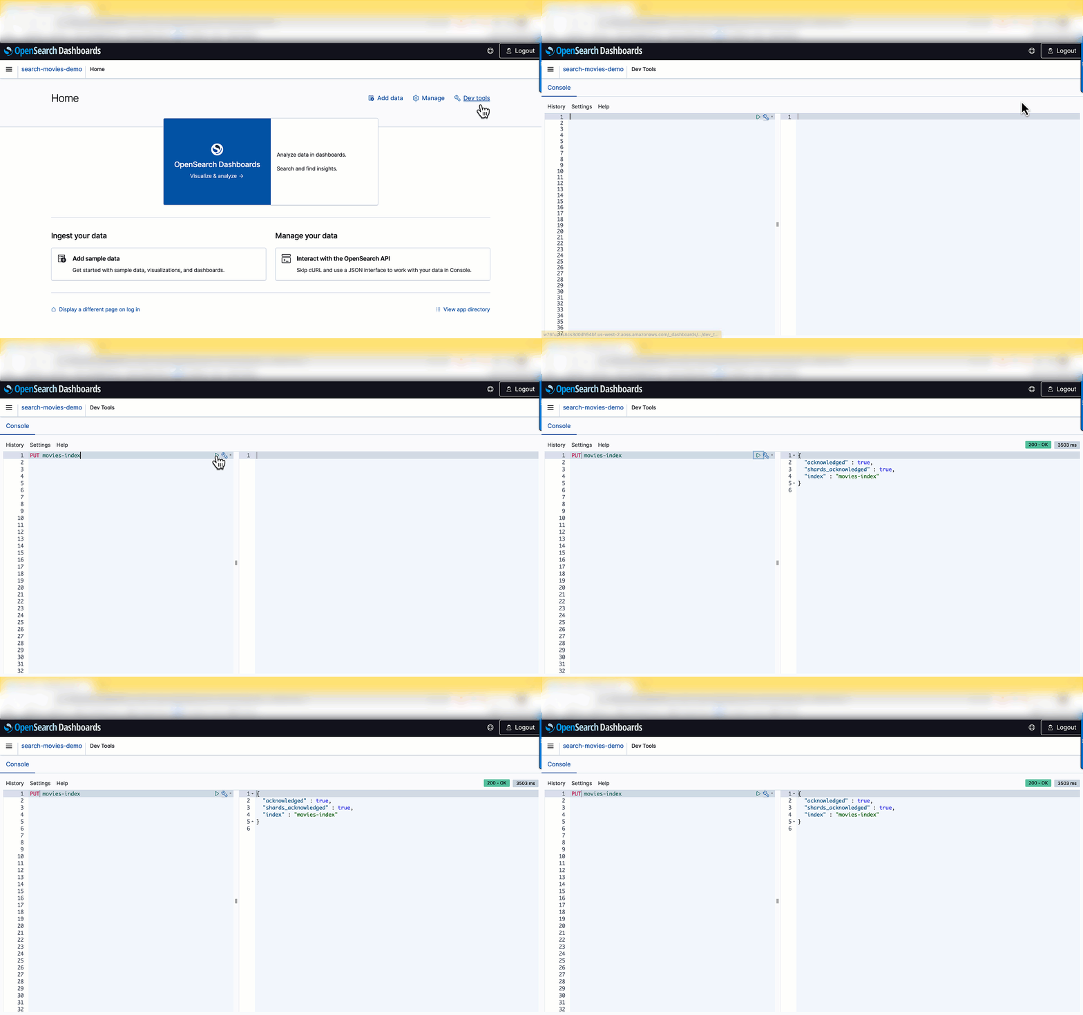
After the index is created, you can ingest documents into the index. OpenSearch provides the option to ingest multiple documents in one request using the \_bulk request. Enter POST /\_bulk in the left pane as shown in the following screenshot, then copy and paste the contents of the sample-movies.bulk file you downloaded earlier.

You have successfully created the movies index and uploaded 1,500 records into the catalog! Now let’s integrate the movie catalog with your search application.
Integrate the Lambda function with an OpenSearch Serverless endpoint
In this step, you create a Lambda function that queries the movie catalog in OpenSearch Serverless and returns the result. For more information, see our tutorial on creating a Lambda function for connecting to and querying an OpenSearch Service domain. You can reuse the same code by replacing the parameters to align to OpenSearch Serverless’s requirements. Replace <my-region> with your corresponding region (for example, us-west-2), use aoss instead of es for service, replace <hostname> with the OpenSearch collection endpoint, and <index-name> with your index (in this case, movies-index).
The following is a snippet of the Lambda code. You can find the complete code in the tutorial.
This Lambda function returns a list of movies based on a search string (such as movie title, director, or actor) provided by the user.
Next, you need to configure the permissions in OpenSearch Serverless’s data access policy to let the Lambda function access the collection.
- On the Lambda console, navigate to your function.
- On the Configuration tab, in the Permissions section, under Execution role, copy the value for Role name.

- Add this role name as one of the principals of your
movie-searchcollection’s data access policy.
Principals can be AWS Identity and Access Management (IAM) users, role ARNs, or SAML identities. These principals must be within the current AWS account.

After you add the role name as a principal, you can see the role ARN updated in your rule, as show in the following screenshot.
Now you can grant collection and index permissions to this principal.
For more details about data access policies, refer to Data access control for Amazon OpenSearch Serverless. Skipping this step or not running it correctly will result in permission errors, and your Lambda code won’t be able to query the movie catalog.

Configure API Gateway
API Gateway acts as a front door for applications to access the code running on Lambda. To create, configure, and deploy the API for the GET method, refer to the steps in the tutorial. For API Gateway to pass the requests to the Lambda function, configure it as a trigger to invoke the Lambda function.
The next step is to integrate it with the front end.
Test the web application
To build the front-end UI, you can download the following sample JavaScript web service. Open the scripts/search.js file and update the apigatewayendpoint variable to point to your API Gateway endpoint:
You can access the front-end application by opening index.html in your browser. When the user runs a query on the front-end application, it calls API Gateway and Lambda to serve up the content hosted in the OpenSearch Serverless collection.

When you search the movie catalog, the Lambda function runs the following query:
The query returns documents based on a provided query string. Let’s look at the parameters used in the query:
- size – The
sizeparameter is the maximum number of documents to return. In this case, a maximum of 25 results is returned. - multi\_match – You use a match query when matching larger pieces of text, especially when you’re using OpenSearch’s relevance to sort your results. With a
multi\_matchquery, you can query across multiple fields specified in the query. - fields – The list of fields you are querying.
In a search for “Harry Potter,” the document with the matching term both in the title and plot fields appears higher than other documents with the matching term only in the title field.

Congratulations! You have configured and deployed a search application fronted by API Gateway, running Lambda functions for the queries served by OpenSearch Serverless.
Clean up
To avoid unwanted charges, delete the OpenSearch Service collection, Lambda function, and API Gateway that you created.
Conclusion
In this post, you learned how to build a simple search application using OpenSearch Serverless. With OpenSearch Serverless, you don’t have to worry about managing the underlying infrastructure. OpenSearch Serverless supports the same ingestion and query APIs as the OpenSearch Project. You can quickly get started by ingesting the data into your OpenSearch Service collection, and then perform searches on the data using your web interface.
In subsequent posts, we dive deeper into many other search queries and features that you can use to make your search application even more effective.
We would love to hear how you are building your search applications today. If you’re just getting started with OpenSearch Serverless, we recommend getting hands-on with the Getting started with Amazon OpenSearch Serverless workshop.
About the authors
 Aish Gunasekar is a Specialist Solutions architect with a focus on Amazon OpenSearch Service. Her passion at AWS is to help customers design highly scalable architectures and help them in their cloud adoption journey. Outside of work, she enjoys hiking and baking.
Pavani Baddepudi is a senior product manager working in search services at AWS. Her interests include distributed systems, networking, and security.
This is a guest post by Jeremy Bristow, Head of Product at Green Flag.
In the US, there’s a saying: “Sooner or later, you’ll break down and call Triple A.” In the UK, that same saying might be “Sooner or later, you’ll break down and call Green Flag.”
Green Flag has been assisting stranded motorists all over Europe for more than 50 years. Having started in the UK in 1971, with the first office located above a fish and chip shop, we have built an expansive network of automobile service providers to assist customers. With that network in place, Green Flag customers need only make a single phone call, or request service via the Green Flag app, to quickly contact a local repair garage, no matter where they’ve broken down.
Green Flag’s commitment to providing world-class service to its customers has consistently earned a Net Promoter Score (NPS) of over 70. We were also recently rated as the top breakdown provider in the H1 2022 UK Customer Satisfaction Index report, which is a national benchmark of customer satisfaction covering 13 sectors and based on 45,000 customer responses.
Unlike most breakdown providers in the UK, Green Flag doesn’t currently own a large fleet of trucks to provide roadside assistance to our 3 million plus customers. Our established network of over 200 locally operated businesses provides in-depth knowledge and expertise related to their specific areas. Our overall mission is simple: “Make motoring stress-free, safe, and simple, for every driver.”
Tech transformation to democratize data
Over the past 4 years, Green Flag has been undertaking a technology transformation with the end goal of enabling data democratization and faster data-driven decisions. This has been a massive undertaking, requiring the business to replace our entire systems architecture, which we’ve done while remaining open 24/7, 365 days a year, maintaining our industry-leading customer service standards and growing the business. Building the plane while flying it is an apt analogy, but it felt more like performing open-heart surgery while running a marathon.
Early on during our tech transformation, we made the decision to develop natively with AWS, using our in-house development team. When it came time to decide on a new business intelligence (BI) tool, it was an easy decision to switch to Amazon QuickSight.
In this post, we discuss what influenced the decision to implement QuickSight and why doing so has made a significant impact on our efficiency and agility.
Changing the game with self-serve insights
Prior to embarking on this transformation, technology had consistently been a blocker to us being able to quickly serve our customers. Our old stack was slow, hard to change, and consistently prevented us from gaining valuable and timely insights from our datasets. We were data rich, but insight poor. It was clear that the status quo was not compatible with our ambitions to grow and trade in an increasingly digital world. We needed a BI tool to bring new and meaningful insights to our data, which would help us leverage our new technologies to deliver meaningful business change.
Although going with QuickSight was an easy decision, we considered the following factors to ensure our needs would be met:
- Alignment to AWS architecture – We didn’t want to invest time and development resources into complicated implementations—we wanted a seamless integration that would cause no headaches.
- Ease of use – We needed an intuitive, user-friendly interface that would make it easy for any user, no matter their tech background or level of expertise in pulling data insights.
- Cost – Affordability is always a concern. With AWS, we can monitor daily usage and the associated costs via our console, so there were never any surprises or hidden costs post-implementation.
Although these considerations were all top of mind, the primary driver for switching to QuickSight is rooted in the data democratization goal within our tech transformation initiative. Providing self-serve access to data and insights to everyone, no matter their tech background, has been a game changer. With QuickSight, we can now present data and insights in a meaningful, easy-to-understand format via near-real-time embedded dashboards that anyone from any tech background can easily build.
Evolving our data culture with QuickSight
Because all employees are now empowered to make data-driven decisions, our data culture has begun to evolve. Having consistent, accurate dashboards that access standardized datasets brings with it a new level of confidence in decision-making. We’re no longer wasting time on discussions about data sources or the risks of inaccuracy. QuickSight and the data governance processes we have built around its use have shifted the discussion to focus on the insights, what they tell us, and what our next steps should be.
The following screenshot shows one of Green Flag’s custom-built dashboards.

Additionally, because QuickSight is so easy to use that self-service requires minimal training and no specialized skills, our data experts can now shift from responding to constant requests for information to focusing on more valuable projects that require their technical depth and expertise. We can now work more efficiently, producing actionable insights that have never before been available, at a pace that enables us to make better decisions, faster.
Mapping our next analytics adventure
The next features that the Green Flag team plan to test and then roll out is Amazon QuickSight Q, which should allow both our data teams and business users to have a more frictionless experience with our data. The feature should enable users to interrogate complex data using simple conversational questions as if they were talking to a colleague, producing results that are then customizable. This will further empower our self-serve strategy by enabling non-technical experts to pose business questions rather than rely on technical expertise and experience.
To learn more about how you can embed customized data visuals, interactive dashboards, and natural language querying into any application, visit Amazon QuickSight Embedded.
About the Author
 Jeremy “Jez” Bristow is Head of Product at Green Flag. He has been working at Green Flag, part of Direct Line Group, for over 4 years and has been co-responsible for delivering the digital transformation programme within Green Flag. They have built a cloud-based ecosystem of micro-services supported by a data platform within AWS to enable the delivery of better customer outcomes to grow their business.
Organizations use their data to solve complex problems by starting small, running iterative experiments, and refining the solution. Although the power of experiments can’t be ignored, organizations have to be cautious about the cost-effectiveness of such experiments. If time is spent creating the underlying infrastructure for enabling experiments, it further adds to the cost.
Developers need an integrated development environment (IDE) for data exploration and debugging of workflows, and different compute profiles for running these workflows. If you choose Amazon EMR for such use cases, you can use an IDE called Amazon EMR Studio for data exploration, transformation, version control, and debugging, and run Spark jobs to process large volume of data. Deploying Amazon EMR on Amazon EKS simplifies management, reduces costs, and improves performance. However, a data engineer or IT administrator needs to spend time creating the underlying infrastructure, configuring security, and creating a managed endpoint for users to connect to. This means such projects have to wait until these experts create the infrastructure.
In this post, we show how a data engineer or IT administrator can use the AWS Analytics Reference Architecture (ARA) to accelerate infrastructure deployment, saving your organization both time and money spent on these data analytics experiments. We use the library to deploy an Amazon Elastic Kubernetes (Amazon EKS) cluster, configure it to use Amazon EMR on EKS, and deploy a virtual cluster and managed endpoints and EMR Studio. You can then either run jobs on the virtual cluster or run exploratory data analysis with Jupyter notebooks on Amazon EMR Studio and Amazon EMR on EKS. The architecture below represent the infrastructure you will deploy with the AWS Analytics Reference Architecture.

Prerequisites
To follow along, you need to have an AWS account that is bootstrapped with the AWS Cloud Development Kit (AWS CDK). For instructions, refer to Bootstrapping. The following tutorial uses TypeScript, and requires version 2 or later of the AWS CDK. If you don’t have the AWS CDK installed, refer to Install the AWS CDK.
Set up an AWS CDK project
To deploy resources using the ARA, you first need to set up an AWS CDK project and install the ARA library. Complete the following steps:
- Create a folder named emr-eks-app:
- Initialize an AWS CDK project in an empty directory and run the following command:
- Install the ARA library:
- In lib/emr-eks-app.ts, import the ARA library as follows. The first line calls the ARA library, the second one defines AWS Identity and Access Management (IAM) policies:
Create and define an EKS cluster and compute capacity
To create an EMR on EKS virtual cluster, you first need to deploy an EKS cluster. The ARA library defines a construct called EmrEksCluster. The construct provisions an EKS cluster, enables IAM roles for service accounts, and deploys a set of supporting controllers like certificate manager controller (needed by the managed endpoint that is used by Amazon EMR Studio) as well as a cluster auto scaler to have an elastic cluster and save on cost when no job is submitted to the cluster.
In lib/emr-eks-app.ts, add the following line:
To learn more about the properties you can customize, refer to EmrEksClusterProps. There are two mandatory parameters in EmrEksCluster construct: The first is eksAdminRoleArn role is mandatory and is the role you use to interact with the Kubernetes control plane. This role must have administrative permissions to create or update the cluster. The second parameter is autoscaling, this parameter allows you to select the autoscaling mechanism, either Karpenter or native Kubernetes Cluster Autoscaler. In this blog we will use Karpenter and we recommend its use due to faster autoscaling, simplified node management and provisioning. Now you’re ready to define the compute capacity.
One way to define worker nodes in Amazon EKS is to use managed node groups. We use one node group called tooling, which hosts the coredns, ingress controller, certificate manager, Karpenter and any other pod that is necessary for the running EMR on EKS jobs or ManagedEndpoint. We also define default Karpenter Provisioners that define capacity to be used for jobs submitted by EMR on EKS. These Provisioners are optimized for different Spark use cases (critical jobs, non-critical job, experimentation and interactive sessions). The construct also allows you to submit your own provisioner defined by a Kubernetes manifest through a method called addKarpenterProvisioner. Let’s discuss the predefined Provisioners.
Default Provisioners configurations
The default provisioners are set for rapid experimentation and are always created by default. However, if you don’t want to use them, you can set the defaultNodeGroups parameter to false in the EmrEksCluster properties at creation time. The Provisioners are defined as follows and are created in each of the subnets that are used by Amazon EKS:
- Critical provisioner – It is dedicated to supporting jobs with aggressive SLAs and are time sensitive. The provisioner uses On-Demand Instances, which aren’t stopped, unlike Spot Instances, and their lifecycle follows through one of the jobs. The nodes use instance stores, which are NVMe disks physically attached to the host, which offer a high I/O throughput that allow better Spark performance, because it’s used as temporary storage for disk spill and shuffle. The instance types used in the node are of the m6gd family. The instances use the AWS Graviton processor, which offers better price/performance than x86 processors. To use this provisioner in your jobs, you can use the following sample configuration, which is referenced in the configuration override of the EMR on EKS job submission.
- Non-critical provisioner – This Provisioner leverage Spot Instances to save costs for jobs that aren’t time sensitive or jobs that are used for experiments. This node use Spot Instances because the jobs aren’t critical and can be interrupted. These instances can be stopped if the instance is reclaimed. The instance types used in the node are of the m6gd family, the driver is On-Demand and executors are on spot instances.
- Notebook provisioner – The Provisioner is for running managed endpoints that are used by Amazon EMR Studio for data exploration using Amazon EMR on EKS. The instances are of t3 family and are On-Demand for driver and Spot Instances for executors to keep the cost low. If the executor instances are stopped, new ones are started by Karpenter. If the executor instances are stopped too often, you can define your own that use On-Demand instances.
The following link provides more details about how each of the provisioner are defined. One import property that is defined in the default Provisioners is there is one for each AZ. This is important because it allows you to reduce inter-AZ network transfer cost when Spark runs a shuffle.
For this post, we use the default Provisioners, so you don’t need to add any lines of code for this section. If you want yo add your own Provisioners you can leverage the method addKarpenterProvisioner to apply your own manifests. You can use helper methods in Utils class like readYamlDocument to read YAML document and loadYaml load YAML files and pass them as arguments to addKarpenterProvisioner method.
Deploy the virtual cluster and an execution role
A virtual cluster is a Kubernetes namespace that Amazon EMR is registered with; when you submit a job, the driver and executor pods are running in the associated namespace. The EmrEksCluster construct offers a method called addEmrVirtualCluster, which creates the virtual cluster for you. The method takes EmrVirtualClusterOptions as a parameter, which has the following attributes:
- name – The name of your virtual cluster.
- createNamespace – An optional field that creates the EKS namespace. This is of type Boolean and by default it doesn’t create a separate EKS namespace, so your virtual cluster is created in the default namespace.
- eksNamespace – The name of the EKS namespace to be linked with the virtual EMR cluster. If no namespace is supplied, the construct uses the default namespace.
- In
lib/emr-eks-app.ts, add the following line to create your virtual cluster:Now we create the execution role, which is an IAM role that is used by the driver and executor to interact with AWS services. Before we can create the execution role for Amazon EMR, we need to first create the
ManagedPolicy. Note that in the following code, we create a policy to allow access to the Amazon Simple Storage Service (Amazon S3) bucket and Amazon CloudWatch logs. - In
lib/emr-eks-app.ts, add the following line to create the policy:If you want to use the AWS Glue Data Catalog, add its permission in the preceding policy.
Now we create the execution role for Amazon EMR on EKS using the policy defined in the previous step using the
createExecutionRoleinstance method. The driver and executor pods can then assume this role to access and process data. The role is scoped in such a way that only pods in the virtual cluster namespace can assume it. To learn more about the condition implemented by this method to restrict access to the role to only pods that are created by Amazon EMR on EKS in the namespace of the virtual cluster, refer to Using job execution roles with Amazon EMR on EKS. - In
lib/emr-eks-app.ts, add the following line to create the execution role:The preceding code produces an IAM role called
execRoleJobwith the IAM policy defined inemrekspolicyand scoped to the namespacedataanalysis. - Lastly, we output parameters that are important for the job run:
Deploy Amazon EMR Studio and provision users
To deploy an EMR Studio for data exploration and job authoring, the ARA library has a construct called NotebookPlatform. This construct allows you to deploy as many EMR Studios as you need (within the account limit) and set them up with the authentication mode that is suitable for you and assign users to them. To learn more about the authentication modes available in Amazon EMR Studio, refer to Choose an authentication mode for Amazon EMR Studio.
The construct creates all the necessary IAM roles and policies needed by Amazon EMR Studio. It also creates an S3 bucket where all the notebooks are stored by Amazon EMR Studio. The bucket is encrypted with a customer managed key (CMK) generated by the AWS CDK stack. The following steps show you how to create your own EMR Studio with the construct.
The notebook platform construct takes NotebookPlatformProps as a property, which allows you to define your EMR Studio, a namespace, the name of the EMR Studio, and its authentication mode.
- In
lib/emr-eks-app.ts, add the following line:For this post, we use IAM users so that you can easily reproduce it in your own account. However, if you have IAM federation or single sign-on (SSO) already in place, you can use them instead of IAM users.To learn more about the parameters of
NotebookPlatformProps, refer to NotebookPlatformProps.Next, we need to create and assign users to the Amazon EMR Studio. For this, the construct has a method called
addUserthat takes a list of users and either assigns them to Amazon EMR Studio in case of SSO or updates the IAM policy to allows access to Amazon EMR Studio for the provided IAM users. The user can also have multiple managed endpoints, and each user can have their Amazon EMR version defined. They can use a different set of Amazon Elastic Compute Cloud (Amazon EC2) instances and different permissions using job execution roles. - In
lib/emr-eks-app.ts, add the following line:In the preceding code, for the sake of brevity, we reuse the same IAM policy that we created in the execution role.
Note that the construct optimizes the number of managed endpoints that are created. If two endpoints have the same name, then only one is created.
- Now that we have defined our deployment, we can deploy it:
You can find a sample project that contains all the steps of the walk through in the following GitHub repository.
When the deployment is complete, the output contains the S3 bucket containing the assets for podTemplate, the link for the EMR Studio, and the EMR Studio virtual cluster ID. The following screenshot shows the output of the AWS CDK after the deployment is complete.

Submit jobs

Because we’re using the default Provisioners, we will use the podTemplate that is defined by the construct available on the ARA GitHub repository. These are uploaded for you by the construct to an S3 bucket called <clustername>-emr-eks-assets; you only need to refer to them in your Spark job. In this job, you also use the job parameters in the output at the end of the AWS CDK deployment. These parameters allow you to use the AWS Glue Data Catalog and implement Spark on Kubernetes best practices like dynamicAllocation and pod collocation. At the end of cdk deploy ARA will output job sample configurations with the best practices listed before that you can use to submit a job. You can submit a job as follows.
A job run is a unit of work such as a Spark JAR file that is submitted to the EMR on EKS cluster. We start a job using the start-job-run command. Note you can use SparkSubmitParameters to specify the Amazon S3 path to the pod template, as shown in the following command:
The code takes the following values:
- <CLUSTER-ID> – The EMR virtual cluster ID
- <SPARK-JOB-NAME> – The name of your Spark job
- <ROLE-ARN> – The execution role you created
- <S3URI-SPARK-JOB> – The Amazon S3 URI of your Spark job
- <S3URI-CRITICAL-DRIVER> – The Amazon S3 URI of the driver pod template, which you get from the AWS CDK output
- <S3URI-CRITICAL-EXECUTOR> – The Amazon S3 URI of the executor pod template
- <Log\_Group\_Name> – Your CloudWatch log group name
- <Log\_Stream\_Prefix> – Your CloudWatch log stream prefix
You can go to the Amazon EMR console to check the status of your job and to view logs. You can also check the status by running the describe-job-run command:
Explore data using Amazon EMR Studio
In this section, we show how you can create a workspace in Amazon EMR Studio and connect to the Amazon EKS managed endpoint from the workspace. From the output, use the link to Amazon EMR Studio to navigate to the EMR Studio deployment. You must sign in with the IAM username you provided in the addUser method.
Create a Workspace
To create a Workspace, complete the following steps:
- Log in to the EMR Studio created by the AWS CDK.
- Choose Create Workspace.
- Enter a workspace name and an optional description.
- Select Allow Workspace Collaboration if you want to work with other Studio users in this Workspace in real time.
- Choose Create Workspace.

After you create the Workspace, choose it from the list of Workspaces to open the JupyterLab environment.

The following screenshot shows what the terminal looks like. For more information about the user interface, refer to Understand the Workspace user interface.

Connect to an EMR on EKS managed endpoint
You can easily connect to the EMR on EKS managed endpoint from the Workspace.
- In the navigation pane, on the Clusters menu, select EMR Cluster on EKS for Cluster type.
The virtual clusters appear on the EMR Cluster on EKS drop-down menu, and the endpoint appears on the Endpoint drop-down menu. If there are multiple endpoints, they appear here, and you can easily switch between endpoints from the Workspace. - Select the appropriate endpoint and choose Attach.

Work with a notebook
You can now open a notebook and connect to a preferred kernel to do your tasks. For instance, you can select a PySpark kernel, as shown in the following screenshot.
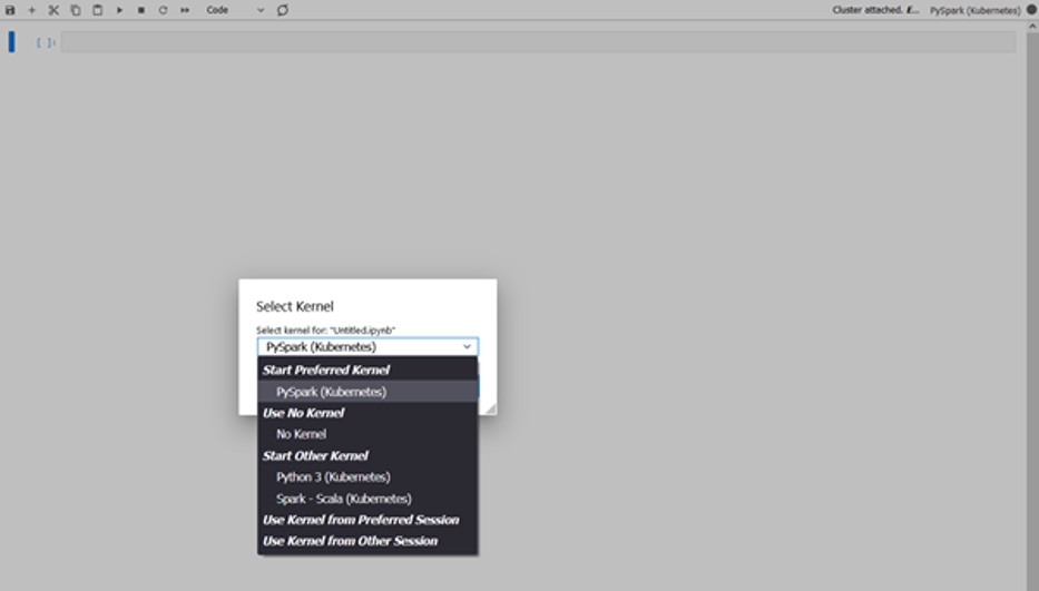
Explore your data
The first step of our data exploration exercise is to create a Spark session and then load the New York taxi dataset from the S3 bucket into a data frame. Use the following code block to load the data into a data frame. Copy the Amazon S3 URI for the location where the dataset resides in Amazon S3.
After we load the data into a data frame, we replace the data of the current\_date column with the actual current date, count the number of rows, and save the data into a Parquet file:
The following screenshot shows the result of our notebook running on Amazon EMR Studio and with PySpark running on Amazon EMR on EKS.

Clean up
To clean up after this post, run cdk destroy.
Conclusion
In this post, we showed how you can use the ARA to quickly deploy a data analytics infrastructure and start experimenting with your data. You can find the full example referenced in this post in the GitHub repository. The AWS Analytics Reference Architecture implements common Analytics pattern and AWS best practices to offer you ready to use constructs to for your experiments. One of the patterns is the data mesh, which you can consult how to use in this blog post.
You can also explore other constructs offered in this library to experiment with AWS Analytics services before transitioning your workload for production.
About the Authors
 Lotfi Mouhib is a Senior Solutions Architect working for the Public Sector team with Amazon Web Services. He helps public sector customers across EMEA realize their ideas, build new services, and innovate for citizens. In his spare time, Lotfi enjoys cycling and running.
 Sandipan Bhaumik is a Senior Analytics Specialist Solutions Architect based in London. He has worked with customers in different industries like Banking & Financial Services, Healthcare, Power & Utilities, Manufacturing and Retail helping them solve complex challenges with large-scale data platforms. At AWS he focuses on strategic accounts in the UK and Ireland and helps customers to accelerate their journey to the cloud and innovate using AWS analytics and machine learning services. He loves playing badminton, and reading books.
The importance of data warehouses and analytics performed on data warehouse platforms has been increasing steadily over the years, with many businesses coming to rely on these systems as mission-critical for both short-term operational decision-making and long-term strategic planning. Traditionally, data warehouses are refreshed in batch cycles, for example, monthly, weekly, or daily, so that businesses can derive various insights from them.
Many organizations are realizing that near-real-time data ingestion along with advanced analytics opens up new opportunities. For example, a financial institute can predict if a credit card transaction is fraudulent by running an anomaly detection program in near-real-time mode rather than in batch mode.
In this post, we show how Amazon Redshift can deliver streaming ingestion and machine learning (ML) predictions all in one platform.
Amazon Redshift is a fast, scalable, secure, and fully managed cloud data warehouse that makes it simple and cost-effective to analyze all your data using standard SQL.
Amazon Redshift ML makes it easy for data analysts and database developers to create, train, and apply ML models using familiar SQL commands in Amazon Redshift data warehouses.
We’re excited to launch Amazon Redshift Streaming Ingestion for Amazon Kinesis Data Streams and Amazon Managed Streaming for Apache Kafka (Amazon MSK), which enables you to ingest data directly from a Kinesis data stream or Kafka topic without having to stage the data in Amazon Simple Storage Service (Amazon S3). Amazon Redshift streaming ingestion allows you to achieve low latency in the order of seconds while ingesting hundreds of megabytes of data into your data warehouse.
This post demonstrates how Amazon Redshift, the cloud data warehouse allows you to build near-real-time ML predictions by using Amazon Redshift streaming ingestion and Redshift ML features with familiar SQL language.
Solution overview
By following the steps outlined in this post, you’ll be able to set up a producer streamer application on an Amazon Elastic Compute Cloud (Amazon EC2) instance that simulates credit card transactions and pushes data to Kinesis Data Streams in real time. You set up an Amazon Redshift Streaming Ingestion materialized view on Amazon Redshift, where streaming data is received. You train and build a Redshift ML model to generate real-time inferences against the streaming data.
The following diagram illustrates the architecture and process flow.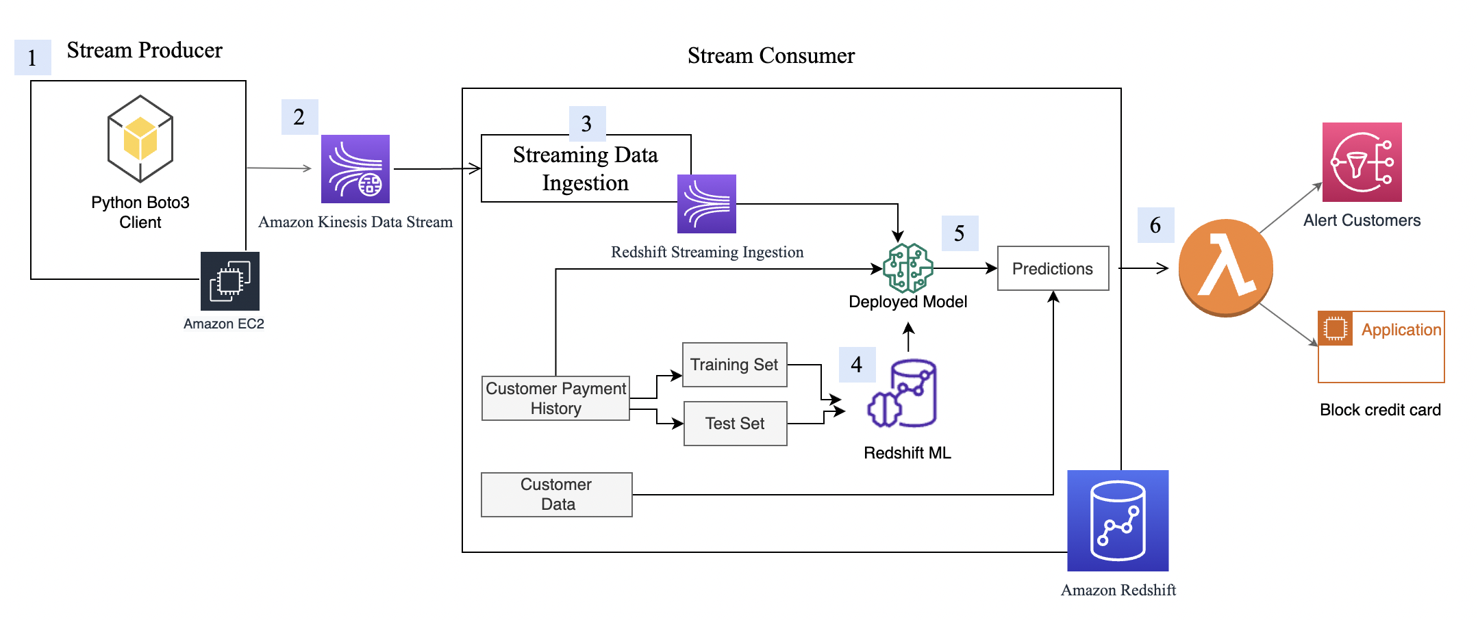
The step-by-step process is as follows:
- The EC2 instance simulates a credit card transaction application, which inserts credit card transactions into the Kinesis data stream.
- The data stream stores the incoming credit card transaction data.
- An Amazon Redshift Streaming Ingestion materialized view is created on top of the data stream, which automatically ingests streaming data into Amazon Redshift.
- You build, train, and deploy an ML model using Redshift ML. The Redshift ML model is trained using historical transactional data.
- You transform the streaming data and generate ML predictions.
- You can alert customers or update the application to mitigate risk.
This walkthrough uses credit card transaction streaming data. The credit card transaction data is fictitious and is based on a simulator. The customer dataset is also fictitious and is generated with some random data functions.
Prerequisites
- Create an Amazon Redshift cluster.
- Configure the cluster to use Redshift ML.
- Create an AWS Identity and Access Management (IAM) user.
- Update the IAM role attached to the Redshift cluster to include permissions to access the Kinesis data stream. For more information about the required policy, refer to Getting started with streaming ingestion.
- Create an m5.4xlarge EC2 instance. We tested Producer application with m5.4xlarge instance but you are free to use other instance type. When creating the instance, use the amzn2-ami-kernel-5.10-hvm-2.0.20220426.0-x86\_64-gp2 AMI.
- To make sure that Python3 is installed in the EC2 instance, run the following command to verity your Python version (note that the data extraction script only works on Python 3):
- Install the following dependent packages to run the simulator program:
- Configure Amazon EC2 using the variables like AWS credentials generated for IAM user created in step 3 above. The following screenshot shows an example using aws configure.
Set up Kinesis Data Streams
Amazon Kinesis Data Streams is a massively scalable and durable real-time data streaming service. It can continuously capture gigabytes of data per second from hundreds of thousands of sources, such as website clickstreams, database event streams, financial transactions, social media feeds, IT logs, and location-tracking events. The data collected is available in milliseconds to enable real-time analytics use cases such as real-time dashboards, real-time anomaly detection, dynamic pricing, and more. We use Kinesis Data Streams because it’s a serverless solution that can scale based on usage.
Create a Kinesis data stream
First, you need to create a Kinesis data stream to receive the streaming data:
- On the Amazon Kinesis console, choose Data streams in the navigation pane.
- Choose Create data stream.
- For Data stream name, enter
cust-payment-txn-stream. - For Capacity mode, select On-demand.

- For the rest of the options, choose the default options and follow through the prompts to complete the setup.
- Capture the ARN for the created data stream to use in the next section when defining your IAM policy.

Set up permissions
For a streaming application to write to Kinesis Data Streams, the application needs to have access to Kinesis. You can use the following policy statement to grant the simulator process that you set up in next section access to the data stream. Use the ARN of the data stream that you saved in the previous step.
Configure the stream producer
Before we can consume streaming data in Amazon Redshift, we need a streaming data source that writes data to the Kinesis data stream. This post uses a custom-built data generator and the AWS SDK for Python (Boto3) to publish the data to the data stream. For setup instructions, refer to Producer Simulator. This simulator process publishes streaming data to the data stream created in the previous step (cust-payment-txn-stream).
Configure the stream consumer
This section talks about configuring the stream consumer (the Amazon Redshift streaming ingestion view).
Amazon Redshift Streaming Ingestion provides low-latency, high-speed ingestion of streaming data from Kinesis Data Streams into an Amazon Redshift materialized view. You can configure your Amazon Redshift cluster to enable streaming ingestion and create a materialized view with auto refresh, using SQL statements, as described in Creating materialized views in Amazon Redshift. The automatic materialized view refresh process will ingest streaming data at hundreds of megabytes of data per second from Kinesis Data Streams into Amazon Redshift. This results in fast access to external data that is quickly refreshed.
After creating the materialized view, you can access your data from the data stream using SQL and simplify your data pipelines by creating materialized views directly on top of the stream.
Complete the following steps to configure an Amazon Redshift streaming materialized view:
- On the IAM console, choose policies in the navigation pane.
- Choose Create policy.
- Create a new IAM policy called
KinesisStreamPolicy. For the streaming policy definition, see Getting started with streaming ingestion. - In the navigation pane, choose Roles.
- Choose Create role.
- Select AWS service and choose Redshift and Redshift customizable.
- Create a new role called
redshift-streaming-roleand attach the policyKinesisStreamPolicy. - Create an external schema to map to Kinesis Data Streams :
Now you can create a materialized view to consume the stream data. You can use the SUPER data type to store the payload as is, in JSON format, or use Amazon Redshift JSON functions to parse the JSON data into individual columns. For this post, we use the second method because the schema is well defined.
- Create the streaming ingestion materialized view
cust\_payment\_tx\_stream. By specifying AUTO REFRESH YES in the following code, you can enable automatic refresh of the streaming ingestion view, which saves time by avoiding building data pipelines:
Note that json\_extract\_path\_text has a length limitation of 64 KB. Also from\_varbye filters records larger than 65KB.
- Refresh the data.
The Amazon Redshift streaming materialized view is auto refreshed by Amazon Redshift for you. This way, you don’t need worry about data staleness. With materialized view auto refresh, data is automatically loaded into Amazon Redshift as it becomes available in the stream. If you choose to manually perform this operation, use the following command:
- Now let’s query the streaming materialized view to see sample data:
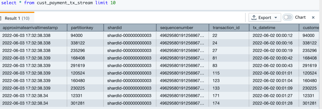
- Let’s check how many records are in the streaming view now:

Now you have finished setting up the Amazon Redshift streaming ingestion view, which is continuously updated with incoming credit card transaction data. In my setup, I see that around 67,000 records have been pulled into the streaming view at the time when I ran my select count query. This number could be different for you.
Redshift ML
With Redshift ML, you can bring a pre-trained ML model or build one natively. For more information, refer to Using machine learning in Amazon Redshift.
In this post, we train and build an ML model using a historical dataset. The data contains a tx\_fraud field that flags a historical transaction as fraudulent or not. We build a supervised ML model using Redshift Auto ML, which learns from this dataset and predicts incoming transactions when those are run through the prediction functions.
In the following sections, we show how to set up the historical dataset and customer data.
Load the historical dataset
The historical table has more fields than what the streaming data source has. These fields contain the customer’s most recent spend and terminal risk score, like number of fraudulent transactions computed by transforming streaming data. There are also categorical variables like weekend transactions or nighttime transactions.
To load the historical data, run the commands using the Amazon Redshift query editor.
Create the transaction history table with the following code. The DDL can also be found on GitHub.
Let’s check how many transactions are loaded:
Check the monthly fraud and non-fraud transactions trend:
Create and load customer data
Now we create the customer table and load data, which contains the email and phone number of the customer. The following code creates the table, loads the data, and samples the table. The table DDL is available on GitHub.
Our test data has about 5,000 customers. The following screenshot shows sample customer data.
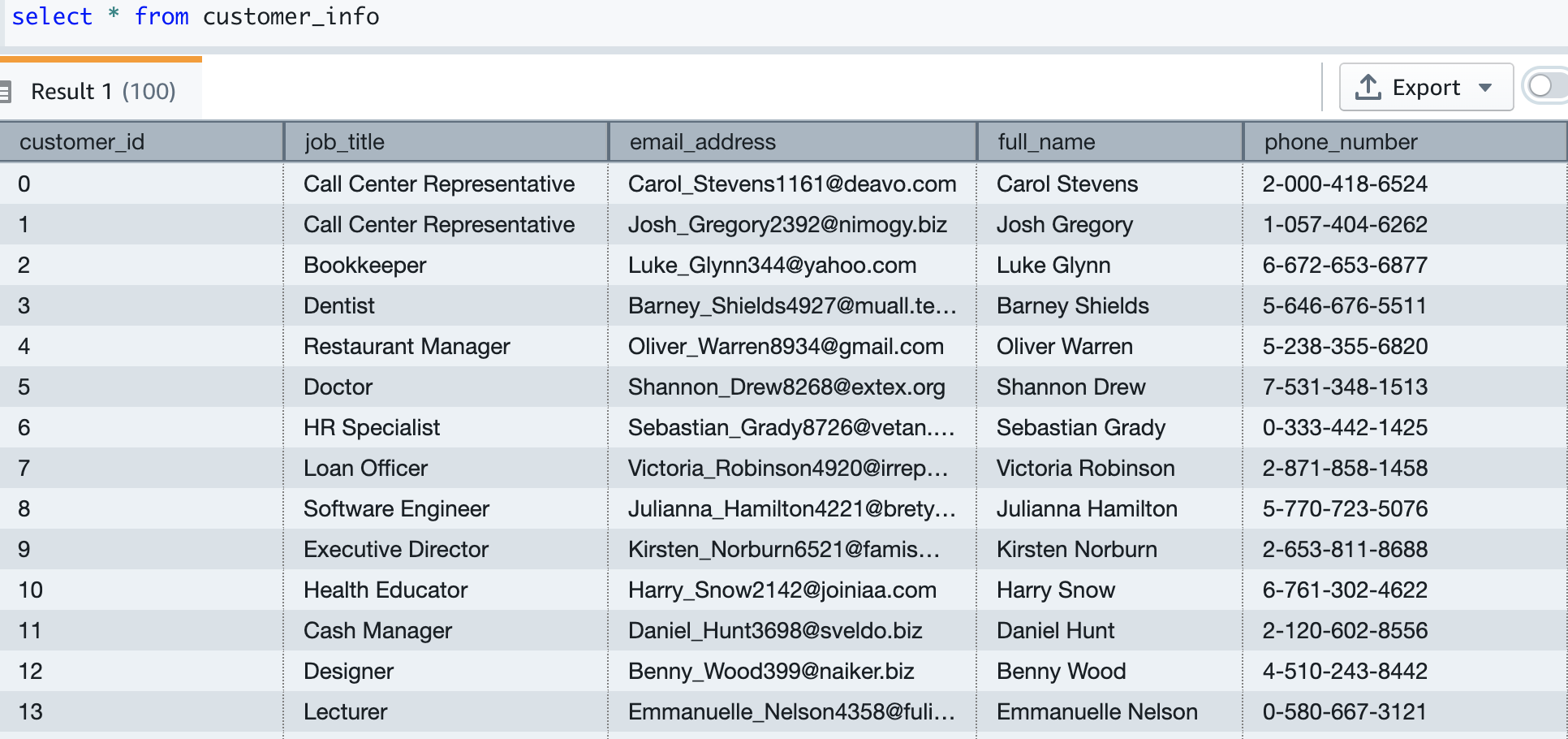
Build an ML model
Our historical card transaction table has 6 months of data, which we now use to train and test the ML model.
The model takes the following fields as input:
We get tx\_fraud as output.
We split this data into training and test datasets. Transactions from 2022-04-01 to 2022-07-31 are for the training set. Transactions from 2022-08-01 to 2022-09-30 are used for the test set.
Let’s create the ML model using the familiar SQL CREATE MODEL statement. We use a basic form of the Redshift ML command. The following method uses Amazon SageMaker Autopilot, which performs data preparation, feature engineering, model selection, and training automatically for you. Provide the name of your S3 bucket containing the code.
I call the ML model as Cust\_cc\_txn\_fd, and the prediction function as fn\_customer\_cc\_fd. The FROM clause shows the input columns from the historical table public.cust\_payment\_tx\_history. The target parameter is set to tx\_fraud, which is the target variable that we’re trying to predict. IAM\_Role is set to default because the cluster is configured with this role; if not, you have to provide your Amazon Redshift cluster IAM role ARN. I set the max\_runtime to 3,600 seconds, which is the time we give to SageMaker to complete the process. Redshift ML deploys the best model that is identified in this time frame.
Depending on the complexity of the model and the amount of data, it can take some time for the model to be available. If you find your model selection is not completing, increase the value for max\_runtime. You can set a max value of 9999.
The CREATE MODEL command is run asynchronously, which means it runs in the background. You can use the SHOW MODEL command to see the status of the model. When the status shows as Ready, it means the model is trained and deployed.
The following screenshots show our output.
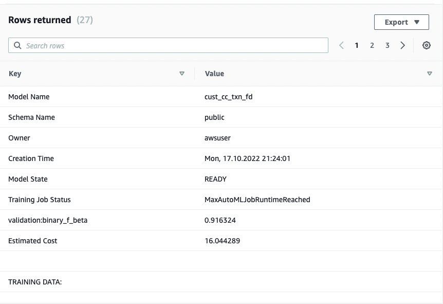
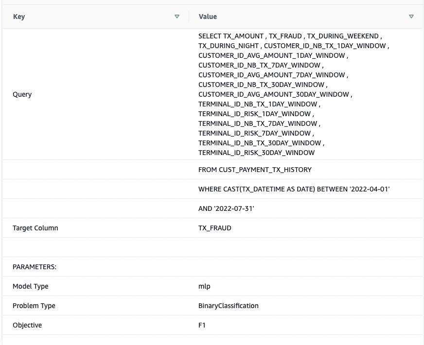
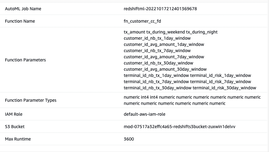
From the output, I see that the model has been correctly recognized as BinaryClassification, and F1 has been selected as the objective. The F1 score is a metric that considers both precision and recall. It returns a value between 1 (perfect precision and recall) and 0 (lowest possible score). In my case, it’s 0.91. The higher the value, the better the model performance.
Let’s test this model with the test dataset. Run the following command, which retrieves sample predictions:
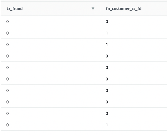
We see that some values are matching and some are not. Let’s compare predictions to the ground truth:
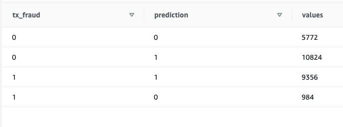
We validated that the model is working and the F1 score is good. Let’s move on to generating predictions on streaming data.
Predict fraudulent transactions
Because the Redshift ML model is ready to use, we can use it to run the predictions against streaming data ingestion. The historical dataset has more fields than what we have in the streaming data source, but they’re just recency and frequency metrics around the customer and terminal risk for a fraudulent transaction.
We can apply the transformations on top of the streaming data very easily by embedding the SQL inside the views. Create the first view, which aggregates streaming data at the customer level. Then create the second view, which aggregates streaming data at terminal level, and the third view, which combines incoming transactional data with customer and terminal aggregated data and calls the prediction function all in one place. The code for the third view is as follows:
Run a SELECT statement on the view:
As you run the SELECT statement repeatedly, the latest credit card transactions go through transformations and ML predictions in near-real time.
This demonstrates the power of Amazon Redshift—with easy-to-use SQL commands, you can transform streaming data by applying complex window functions and apply an ML model to predict fraudulent transactions all in one step, without building complex data pipelines or building and managing additional infrastructure.
Expand the solution
Because the data streams in and ML predictions are made in near-real time, you can build business processes for alerting your customer using Amazon Simple Notification Service (Amazon SNS), or you can lock the customer’s credit card account in an operational system.
This post doesn’t go into the details of these operations, but if you’re interested in learning more about building event-driven solutions using Amazon Redshift, refer to the following GitHub repository.
Clean up
To avoid incurring future charges, delete the resources that were created as part of this post.
Conclusion
In this post, we demonstrated how to set up a Kinesis data stream, configure a producer and publish data to streams, and then create an Amazon Redshift Streaming Ingestion view and query the data in Amazon Redshift. After the data was in the Amazon Redshift cluster, we demonstrated how to train an ML model and build a prediction function and apply it against the streaming data to generate predictions near-real time.
If you have any feedback or questions, please leave them in the comments.
About the Authors
 Bhanu Pittampally is an Analytics Specialist Solutions Architect based out of Dallas. He specializes in building analytic solutions. His background is in data warehouses—architecture, development, and administration. He has been in the data and analytics field for over 15 years.
 Praveen Kadipikonda is a Senior Analytics Specialist Solutions Architect at AWS based out of Dallas. He helps customers build efficient, performant, and scalable analytic solutions. He has worked with building databases and data warehouse solutions for over 15 years.
 Ritesh Kumar Sinha is an Analytics Specialist Solutions Architect based out of San Francisco. He has helped customers build scalable data warehousing and big data solutions for over 16 years. He loves to design and build efficient end-to-end solutions on AWS. In his spare time, he loves reading, walking, and doing yoga.
Novo Nordisk is a leading global pharmaceutical company, responsible for producing life-saving medicines that reach more than 34 million patients each day. They do this following their triple bottom line—that they must strive to be environmentally sustainable, socially sustainable, and financially sustainable. The combination of using AWS and data supports all these targets.
Data is pervasive throughout the entire value chain of Novo Nordisk. From foundational research, manufacturing lines, sales and marketing, clinical trials, pharmacovigilance, through patient-facing data-driven applications. Therefore, getting the foundation around how data is stored, safeguarded, and used in a way that provides the most value is one of the central drivers of improved business outcomes.
Together with AWS Professional Services, we’re building a data and analytics solution using a modern data architecture. The collaboration between Novo Nordisk and AWS Professional Services is a strategic and long-term close engagement, where developers from both organizations have worked together closely for years. The data and analytics environments are built around of the core tenets of the data mesh—decentralized domain ownership of data, data as a product, self-service data infrastructure, and federated computational governance. This enables the users of the environment to work with data in the way that drives the best business outcomes. We have combined this with elements from evolutionary architectures that will allow us to adapt different functionalities as AWS continuously develops new services and capabilities.
In this series of posts, you will learn how Novo Nordisk and AWS Professional Services built a data and analytics ecosystem to speed up innovation at petabyte scale:
- In this first post, you will learn how the overall design has enabled the individual components to come together in a modular way. We dive deep into how we built a data management solution based on the data mesh architecture.
- The second post discusses how we built a trust network between the systems that comprise the entire solution. We show how we use event-driven architectures, coupled with the use of attribute-based access controls, to ensure permission boundaries are respected at scale.
- In the third post, we show how end-users can consume data from their tool of choice, without compromising data governance. This includes how to configure Okta, AWS Lake Formation, and Microsoft Power BI to enable SAML-based federated use of Amazon Athena for an enterprise business intelligence (BI) activity.
Pharma-compliant environment
As a pharmaceutical industry, GxP compliance is a mandate for Novo Nordisk. GxP is a general abbreviation for the “Good x Practice” quality guidelines and regulations defined by regulators such as European Medicines Agency, U.S. Food and Drug Administration, and others. These guidelines are designed to ensure that medicinal products are safe and effective for their intended use. In the context of a data environment, GxP compliance involves implementing integrity controls for data used to in decision making and processes and is used to guide how change management processes are implemented to continuously ensure compliance over time.
Because this data environment supports teams across the whole organization, each individual data owner must retain accountability on their data. Features were designed to provide data owners autonomy and transparency when managing their data, enabling them to take this responsibility. This includes the capability to handle personally identifiable information (PII) data and other sensitive workloads. To provide traceability on the environment, audit capabilities were added, which we describe more in this post.
Solution overview
The full solution is a sprawling landscape of independent services that work together to enable data and analytics with a decentralized data governance model at petabyte scale. Schematically, it can be represented as in the following figure.
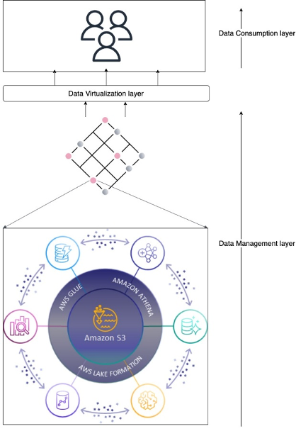
The architecture is split into three independent layers: data management, virtualization, and consumption. The end-user sits in the consumption layer and works with their tool of choice. It’s meant to abstract as much of the AWS-native resources to application primitives. The consumption layer is integrated into the virtualization layer, which abstracts the access to data. The purpose of the virtualization layer is to translate between data consumption and data management solutions. The access to data is managed by what we refer to as data management solutions. We discuss one of our versatile data management solutions later in this post. Each layer in this architecture is independent of each other and instead only relies on well-defined interfaces.
Central to this architecture is that access is encapsulated in an AWS Identity and Access Management (IAM) role session. The data management layer focuses on providing the IAM role with the right permissions and governance, the virtualization layer provides access to the role, and the consumption layer abstracts the use of the roles in the tools of choice.
Technical architecture
Each of the three layers in the overall architecture has a distinct responsibility, but no singular implementation. Think of them as abstract classes. They can be implemented in concrete classes, and in our case they rely on foundational AWS services and capabilities. Let’s go through each of the three layers.
Data management layer
The data management layer is responsible for providing access to and governance of data. As illustrated in the following diagram, a minimal construct in the data management layer is the combination of an Amazon Simple Storage Service (Amazon S3) bucket and an IAM role that gives access to the S3 bucket. This construct can be expanded to include granular permission with Lake Formation, auditing with AWS CloudTrail, and security response capabilities from AWS Security Hub. The following diagram also shows that a single data management solution has no singular span. It can cross many AWS accounts and be comprised of any number of IAM role combinations.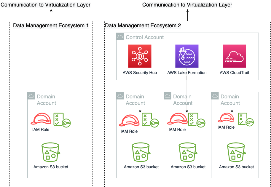
We have purposely not illustrated the trust policy of these roles in this figure, because those are a collaborative responsibility between the virtualization layer and the data management layer. We go into detail of how that works in the next post in this series. Data engineering professionals often interface directly with the data management layer, where they curate and prepare data for consumption.
Virtualization layer
The purpose of the virtualization layer is to keep track of who can do what. It doesn’t have any capabilities in itself, but translates the requirements from the data management ecosystems to the consumption layers and vice versa. It enables end-users on the consumption layer to access and manipulate data on one or more data management ecosystems, according to their permissions. This layer abstracts from end-users the technical details on data access, such as permission model, role assumptions, and storage location. It owns the interfaces to the other layers and enforces the logic of the abstraction. In the context of hexagonal architectures (see Developing evolutionary architecture with AWS Lambda), the interface layer plays the role of the domain logic, ports, and adapters. The other two layers are actors. The data management layer communicates the state of the layer to the virtualization layer and conversely receives information about the service landscape to trust. The virtualization layer architecture is shown in the following diagram.
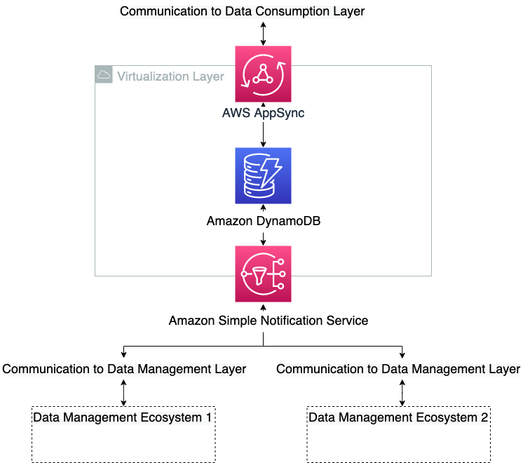
Consumption layer
The consumption layer is where the end-users of the data products are sitting. This can be data scientists, business intelligence analysts, or any third party that generates value from consuming the data. It’s important for this type of architecture that the consumption layer has a hook-based sign-in flow, where the authorization into the application can be modified at sign-in time. This is to translate the AWS-specific requirement into the target applications. After the session in the client-side application has successfully been started, it’s up to the application itself to instrument for data layer abstraction, because this will be application specific. And this is an additional important decoupling, where some responsibility is pushed to the decentralized units. Many modern software as a service (SaaS) applications support these built-in mechanisms, such as Databricks or Domino Data Lab, whereas more traditional client-side applications like RStudio Server have more limited native support for this. In the case where native support is missing, a translation down to the OS user session can be done to enable the abstraction. The consumption layer is shown schematically in the following diagram.
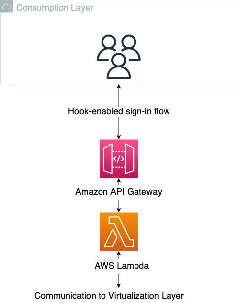
When using the consumption layer as intended, the users don’t know that the virtualization layer exists. The following diagram illustrates the data access patterns.
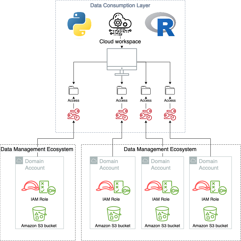
Modularity
One of the main advantages of adopting the hexagonal architecture pattern, and delegating both the consuming layer and the data management layer to primary and secondary actors, means that they can be changed or replaced as new functionalities are released that require new solutions. This gives a hub-and-spoke type pattern, where many different types of producer/consumer type systems can be connected and work simultaneously in union. An example of this is that the current solution running in Novo Nordisk supports multiple, simultaneous data management solutions and are exposed in a homogenous way in the consuming layer. This includes both a data lake, the data mesh solution presented in this post, and several independent data management solutions. And these are exposed to multiple types of consuming applications, from custom managed, self-hosted applications, to SaaS offerings.
Data management ecosystem
To scale the usage of the data and increase the freedom, Novo Nordisk, jointly with AWS Professional Services, built a data management and governance environment, named Novo Nordisk Enterprise DataHub (NNEDH). NNEDH implements a decentralized distributed data architecture, and data management capabilities such as an enterprise business data catalog and data sharing workflow. NNEDH is an example of a data management ecosystem in the conceptual framework introduced earlier.
Decentralized architecture: From a centralized data lake to a distributed architecture
Novo Nordisk’s centralized data lake consists of 2.3 PB of data from more than 30 business data domains worldwide serving over 2000+ internal users throughout the value chain. It has been running successfully for several years. It is one of the data management ecosystems currently supported.
Within the centralized data architecture, data from each data domain is copied, stored, and processed in one central location: a central data lake hosted in one data storage. This pattern has challenges at scale because it retains the data ownership with the central team. At scale, this model slows down the journey toward a data-driven organization, because ownership of the data isn’t sufficiently anchored with the professionals closest to the domain.
The monolithic data lake architecture is shown in the following diagram.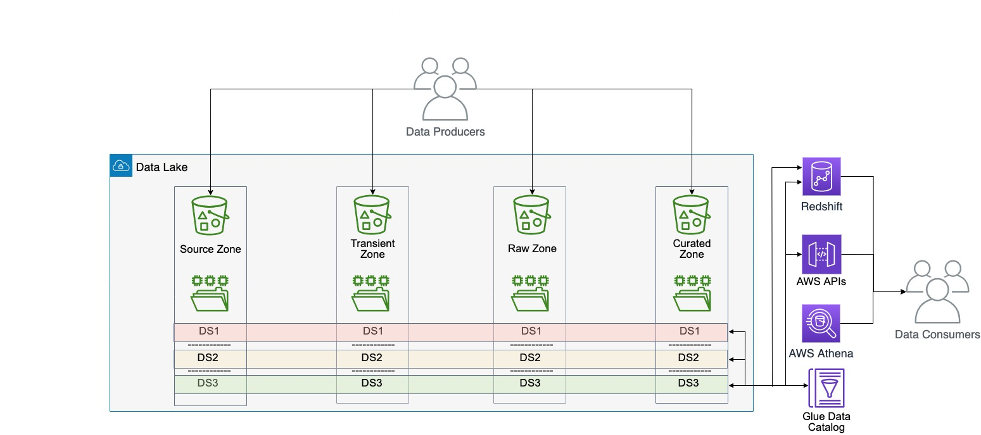
Within the decentralized distributed data architecture, the data from each domain is kept within the domain on its own data storage and compute account. In this case, the data is kept close to domain experts, because they’re the ones who know their own data best and are ultimately the owner of any data products built around their data. They often work closely with business analysts to build the data product and therefore know what good data means to consumers of their data products. In this case, the data responsibility is also decentralized, where each domain has its own data owner, putting the accountability onto the true owners of the data. Nevertheless, this model might not work at small scale, for example an organization with only one business unit and tens of users, because it would introduce more overhead on the IT team to manage the organization data. It better suits large organizations, or small and medium ones that would like to grow and scale.
The Novo Nordisk data mesh architecture is shown in the following diagram.
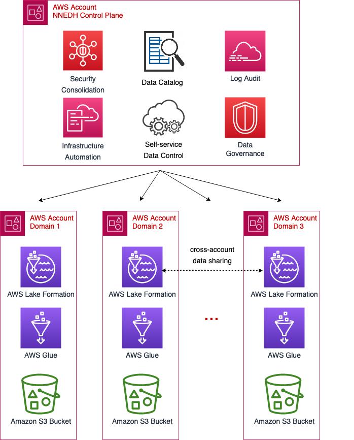
Data domains and data assets
To enable the scalability of data domains across the organization, it’s mandatory to have a standard permission model and data access pattern. This standard must not be too restrictive in such a way that it may be a blocker for specific use cases, but it should be standardized in such a way to use the same interface between the data management and virtualization layers.
The data domains on NNEDH are implemented by a construct called an environment. An environment is composed of at least one AWS account and one AWS Region. It’s a workplace where data domain teams can work and collaborate to build data products. It links the NNEDH control plane to the AWS accounts where the data and compute of the domain reside. The data access permissions are also defined at the environment level, managed by the owner of the data domain. The environments have three main components: a data management and governance layer, data assets, and optional blueprints for data processing.
For data management and governance, the data domains rely on Lake Formation, AWS Glue, and CloudTrail. The deployment method and setup of these components is standardized across data domains. This way, the NNEDH control plane can provide connectivity and management to data domains in a standardized way.
The data assets of each domain residing in an environment are organized in a dataset, which is a collection of related data used for building a data product. It includes technical metadata such as data format, size, and creation time, and business metadata such as the producer, data classification, and business definition. A data product can use one or several datasets. It is implemented through managed S3 buckets and the AWS Glue Data Catalog.
Data processing can be implemented in different ways. NNEDH provides blueprints for data pipelines with predefined connectivity to data assets to speed up the delivery of data products. Data domain users have the freedom to use any other compute capability on their domain, for example using AWS services not predefined on the blueprints or accessing the datasets from other analytics tools implemented in the consumption layer, as mentioned earlier in this post.
Data domain personas and roles
On NNEDH, the permission levels on data domains are managed through predefined personas, for example data owner, data stewards, developers, and readers. Each persona is associated with an IAM role that has a predefined permission level. These permissions are based on the typical needs of users on these roles. Nevertheless, to give more flexibility to data domains, these permissions can be customized and extended as needed.
The permissions associated with each persona are related only to actions allowed on the AWS account of the data domain. For the accountability on data assets, the data access to the assets is managed by specific resource policies instead of IAM roles. Only the owner of each dataset, or data stewards delegated by the owner, can grant or revoke data access.
On the dataset level, a required persona is the data owner. Typically, they work closely with one or many data stewards as data products managers. The data steward is the data subject matter expert of the data product domain, responsible for interpreting collected data and metadata to derive deep business insights and build the product. The data steward bridges between business users and technical teams on each data domain.
Enterprise business data catalog
To enable freedom and make the organization data assets discoverable, a web-based portal data catalog is implemented. It indexes in a single repository metadata from datasets built on data domains, breaking data silos across the organization. The data catalog enables data search and discovery across different domains, as well as automation and governance on data sharing.
The business data catalog implements data governance processes within the organization. It ensures the data ownership—someone in the organization is responsible for the data origin, definition, business attributes, relationships, and dependencies.
The central construct of a business data catalog is a dataset. It’s the search unit within the business catalog, having both technical and business metadata. To collect technical metadata from structured data, it relies on AWS Glue crawlers to recognize and extract data structures from the most popular data formats, including CSV, JSON, Avro, and Apache Parquet. It provides information such as data type, creation date, and format. The metadata can be enriched by business users by adding a description of the business context, tags, and data classification.
The dataset definition and related metadata are stored in an Amazon Aurora Serverless database and Amazon OpenSearch Service, enabling you to run textual queries on the data catalog.
Data sharing
NNEDH implements a data sharing workflow, enabling peer-to-peer data sharing across AWS accounts using Lake Formation. The workflow is as follows:
- A data consumer requests access to the dataset.
- The data owner grants access by approving the access request. They can delegate the approval of access requests to the data steward.
- Upon the approval of an access request, a new permission is added to the specific dataset in Lake Formation of the producer account.
The data sharing workflow is shown schematically in the following figure.
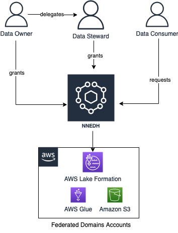
Security and audit
The data in the Novo Nordisk data mesh lies in AWS accounts owned by Novo Nordisk business accounts. The configuration and the states of the data mesh are stored in Amazon Relational Database Service (Amazon RDS). The Novo Nordisk security architecture is shown in the following figure.
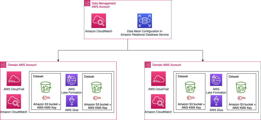
Access and edits to the data in NNEDH needs to be logged for audit purposes. We need to be able to tell who modified data, when the modification happened, and what modifications were applied. In addition, we need to be able to answer why the modification was allowed by that person at that time.
To meet these requirements, we use the following components:
- CloudTrail to log API calls. We specifically enable CloudTrail data event logging for S3 buckets and objects. By activating the logging, we can trace back any modification to any files in the data lake to the person who made the modification. We enforce usage of source identity for IAM role sessions to ensure user traceability.
- We use Amazon RDS to store the configuration of the data mesh. We log queries against the RDS database. Together with CloudTrail, this log allows us to answer the question of why a modification to a file in Amazon S3 at a specific time by a specific person is possible.
- Amazon CloudWatch to log activities across the mesh.
In addition to those logging mechanisms, the S3 buckets are created using the following properties:
- The bucket is encrypted using server-side encryption with AWS Key Management Service (AWS KMS) and customer managed keys
- Amazon S3 versioning is activated by default
Access to the data in NNEDH is controlled at the group level instead of individual users. The group corresponds to the group defined in the Novo Nordisk directory group. To keep track of the person who modified the data in the data lakes, we use the source identity mechanism explained in the post How to relate IAM role activity to corporate identity.
Conclusion
In this post, we showed how Novo Nordisk built a modern data architecture to speed up the delivery of data-driven use cases. It includes a distributed data architecture, to scale the usage to petabyte scale for over 2,000 internal users throughout the value chain, as well as a distributed security and audit architecture handling data accountability and traceability on the environment to meet their compliance requirements.
The next post in this series describes the implementation of distributed data governance and control at scale of Novo Nordisk’s modern data architecture.
About the Authors
 Jonatan Selsing is former research scientist with a PhD in astrophysics that has turned to the cloud. He is currently the Lead Cloud Engineer at Novo Nordisk, where he enables data and analytics workloads at scale. With an emphasis on reducing the total cost of ownership of cloud-based workloads, while giving full benefit of the advantages of cloud, he designs, builds, and maintains solutions that enable research for future medicines.
Hassen Riahi is a Sr. Data Architect at AWS Professional Services. He holds a PhD in Mathematics & Computer Science on large-scale data management. He works with AWS customers on building data-driven solutions.
 Anwar Rizal is a Senior Machine Learning consultant based in Paris. He works with AWS customers to develop data and AI solutions to sustainably grow their business.
Moses Arthur comes from a mathematics and computational research background and holds a PhD in Computational Intelligence specialized in Graph Mining. He is currently a Cloud Product Engineer at Novo Nordisk building GxP-compliant enterprise data lakes and analytics platforms for Novo Nordisk global factories producing digitalized medical products.
 Alessandro Fior is a Sr. Data Architect at AWS Professional Services. With over 10 years of experience delivering data and analytics solutions, he is passionate about designing and building modern and scalable data platforms that accelerate companies to get value from their data.
 Kumari Ramar is an Agile certified and PMP certified Senior Engagement Manager at AWS Professional Services. She delivers data and AI/ML solutions that speed up cross-system analytics and machine learning models, which enable enterprises to make data-driven decisions and drive new innovations.
Convoy is the leading digital freight network in the United States. We move millions of truckloads around the country through our connected network of carriers, saving money for shippers, increasing earnings for drivers, and eliminating carbon waste for our planet. In 2015, Convoy started a movement toward efficient freight. We build technology to find smarter ways to connect shippers with carriers while solving some of the toughest problems that result in waste in the freight industry.
As a digital freight network, Convoy uses machine learning and automation to efficiently connect shippers and carriers. As our marketplace grows, it creates a flywheel effect that benefits both sides. As more shippers join the network, drivers have better options, fewer empty miles, and fewer wasted hours, allowing them to earn more per day. As more carriers join the network, capacity increases and shippers see lower costs and higher service quality. Convoy is on a mission to transport the world with endless capacity and zero waste.
Our digital freight network collects thousands of disparate data points and intelligently connects the dots to provide transparent visibility into freight operations. By providing transparency and insights into every step of the shipment lifecycle, shippers benefit from lower costs, reduced waste, and higher carrier loyalty. To surface these insights to customers inside our product, we needed a business intelligence (BI) tool that could not only handle our volume of data, but could provide at-a-glance insights through a user-friendly interface, empowering our customers to make data-driven decisions, and taking the guesswork out of resolving unexpected issues.
After reviewing our options and evaluating which would best meet our needs, we turned to Amazon QuickSight.
In this post, we discuss how QuickSight is helping us serve our customers with the insights they need, and why we consider this business decision a win for Convoy.
From disparate data points to at-a-glance insights
Our vast network of small carriers and owner-operators, totaling more than 400,000 trucks nationwide, provides meaningful data points through the Convoy app. We require carriers to use our app when hauling loads—this is how we provide GPS tracking on 95% of live loads and 100% of drop loads. It’s also how we collect robust data around dwell times, detention costs, and more. To date, we’ve captured more than 2.7 million facility reviews in the Convoy app.
We chose QuickSight because we needed ease in development. We wanted to be able to quickly build dashboards and get them in the hands of our customers. Because this is an externally facing tool, we had data privacy and governance requirements to consider as well. Especially important was that we needed granularity in row-level security. QuickSight provided what we needed out of the box, whereas the other BI platforms we considered did not. Additionally, QuickSight’s pricing would allow us to scale the platform as our user base continues to grow.
Connecting the dots with data
The challenges facing our customers are as varied as the landscapes our carriers travel through every day. From managing delays due to weather, traffic, and unpredictable load times on the carrier’s end, to lacking freight visibility and root causes of operational issues and inaccuracies in manual reporting on the shipper’s end, there is no shortage of opportunities to improve the status quo.
The following screenshot shows performance metrics, like dwell time and incidentals per shipment, plus breakouts that show incidental types and categories for each facility.

Where we strive to meet the needs of both shippers and carriers, we’re in a unique position to connect the dots to identify gaps on one end that have corresponding inputs on the other. The challenges shippers face are often driven by pricing, complexity, and reliability of transporting goods. For carriers, their challenges are more centered on earning predictable and consistent income with the least amount of time and effort invested in finding loads, building schedules, and adjusting to delays. Our customers have sophisticated internal analytics programs, but highly granular data or synthesized data from their vendors is rare. Finding ways to develop metrics and benchmarks for specific business entities (lanes, regions, facilities, and so on) meant we would need to learn and update our products quickly. QuickSight allows us to do that.
With so many data points and opportunities to turn them into key insights, the dashboards and visualizations QuickSight provides makes spotting trends and taking proactive measures to get ahead of minor issues before they become major problems easier than ever.
When reviewing our BI options, the following factors were front and center in our decision to go with QuickSight:
- Pace of development – We wanted to deliver insights to our customers quickly. The seamless integration of QuickSight with other AWS services had our dashboards up and running in no time.
- Secure access to data – With row-level authorization, QuickSight gives us the flexibility we need, along with the peace of mind knowing the data is secure.
- Scalable cost model – The QuickSight pricing model suits our needs, allowing us to scale based on usage.
When we first piloted our external insights product, we built a prototype with our previously used BI tool. Building future iterations with this same tool wasn’t feasible because it lacked functionality in several key areas. We needed to be able to join data from multiple sources, drill down into layers of data, and customize data based on the user accessing the information. In addition, because we were self-hosting, the overhead of scaling our footprint was going to be high. We did consider other solutions, but QuickSight was best able to offer all the features we needed, at the best price.
Visibility improves efficiency
With QuickSight, we were able to build an external-facing product for our shipper customers, helping them gain visibility into the health of their supply chain, which could then provide insights to make things run more efficiently.
The following screenshot shows incidentals, broken out by spend, type or category, and more.

With a visualization of how incidental costs break down, for example, they can see the cost of having a truck unloaded at a facility, the cost of canceling loads on a driver, the cost of having travers waiting at a facility, and more. With that visibility, our shipper customers can now begin to address systemic issues that can save them money, such as improving scheduling to reduce driver wait times.
The following screenshot shows a visualization on carrier feedback, which shippers could use to make improvements that provide a faster, smoother experience.

Future plans with partnering team expansions
They say that imitation is the purest form of flattery. Although that phrase is often used in the context of competitors who develop products and services that are suspiciously similar to an existing product or service, it can also apply to when good ideas are duplicated within an organization. That’s the case for us, in that our QuickSight adoption has drawn the attention and curiosity of partnering teams, who have reached out to us to understand our implementation specifics and the successes we’ve seen as a result.
We’re very happy with our QuickSight Embedded experience and look forward to continuing to iterate and expand its use for additional customer profiles and use cases.
To learn more about how you can embed customized data visuals, interactive dashboards, and natural language querying into any application, visit Amazon QuickSight Embedded.
About the Author
 Dorothy Li is Convoy’s CTO, overseeing Convoy’s Product and Engineering group and technology strategy, shaping and scaling the company’s innovation and industry-defining technology platforms. Prior to Convoy, Dorothy held leadership roles at Amazon, most recently as Vice President of BI and Analytics at AWS. During her more than 20 years at Amazon, Dorothy helped build out Amazon’s ecommerce platform and also led and collaborated on products that had visibly impacted customers around the world – from the initial launch of Amazon Prime, to Kindle, and at AWS where she focused on data analytics and BI. Dorothy received her Bachelor of Science at Brigham Young University and studies at Shanghai International Studies University.
Amazon Identity Services is responsible for the way Amazon customers—buyers, sellers, developers—identify themselves on Amazon. Our team also manages customers’ core account information, such as names and delivery addresses. Our mission is to deliver the most intuitive, convenient, and secure authentication experience. We’re in charge of account security for Amazon, worldwide, on all device surfaces.
Identity systems make millions of security decisions per second. We ingest datasets at a large scale—processing 9 TB per hour—and produce analytical datasets that grow by billions of rows per hour. Our core business metrics within the Amazon Identity Services team are built on top of these datasets, which we use for leadership meetings, product launch decisions, metric movement investigations, and discovering new innovation opportunities to simplify security experiences for our customers.
In this post, we discuss how we use Amazon QuickSight to empower partners with self-serve data discovery.
Inaccessible insights block data-driven decisions
The sheer volume of our datasets made gathering insights a slow process. Not only that, but datasets weren’t accessible to a wide audience outside our team, such as partners, program managers, product managers, and so on. As a result, Business Intelligence Engineers (BIEs) spent a lot of time writing ad hoc queries, which then took a long time to run. When the insights were ready, BIEs were tasked with answering questions via manual processes that didn’t scale.
We chose QuickSight to not only speed up our processing times, but to create efficiencies with self-serve insight access via analyses (exploration and authoring) and dashboards for consumption. With partners and stakeholders having the ability to access insights without assistance, our BIEs were able to shift focus from ad hoc requests to more impactful projects that were a better use of their skills and expertise.
In the following sections, we discuss what we were looking for in BI capabilities, and how QuickSight satisfied those requirements for our team.
Removing the middle person with QuickSight
Imagine being the pilot of a commercial airline, navigating in cloudy conditions. You know your destination lies ahead, but you can’t see it; you have to rely on your dashboard of instruments to navigate so you’ll arrive safely. It’s similar when working on large-scale consumer products. Although our team gathers anecdotes and reviews feedback to form hypotheses on what our customers need, only by analyzing data at scale can we truly understand customer problems and design appropriate solutions.
The status quo that positioned our BIEs between stakeholders and the insights that were needed required a manual, error-prone process, with a time-to-insight that could take weeks. Even more problematic was that insights were limited to what the requestor envisioned. There was no flexibility to explore and visualize data with a simple drag-and-drop UI. This inability to explore and interact with available data meant stakeholders didn’t know the best questions to ask. Our team needed to make data more accessible to partner teams and non-BIE users, and we needed that access to be fast, intuitive, and to provide a single, indisputable source of truth.
With our research into BI tool options, we were looking for the following:
- Accessible insights – We needed to ensure users from all levels of technical experience would be able to access and understand the insights provided to them
- Speed – With an ingestion rate of 9 TB of data per hour, we needed our BI tool to be fast and reliable
- Security – Built-in row-level and column-level security would give us the ability to provide on-demand access to thousands of users across AWS
The first option we considered had a lot of great features, but it wouldn’t scale without a server. The next option we looked at was very capable in a lot of areas, but it wouldn’t be as accessible for non-BIE users, and it also required a team to manage a server. QuickSight was a great fit because it’s not only serverless, but also has enough visualization capabilities to make it useful for self-service data.
QuickSight also offered seamless integration with Amazon Redshift, and the ability to publish our business metrics to QuickSight SPICE (Super-fast, Parallel, In-memory Calculation Engine), its robust in-memory engine. SPICE performs rapid advanced calculations and serves data. What we love most about SPICE is that it greatly reduces time-to-insight, supports column-level security for staying in compliance, and most importantly it’s super fast for data exploration within analyses.
Self-service data discovery just a few clicks away
Publishing our metrics to QuickSight SPICE enabled us to create pre-authored dashboards, and empowered users to create their own analytical content via analyses. Our technical program managers have all been trained on how to use QuickSight to create visualizations, whereas our BIE team members are dedicating their time to creating better datasets. Our non-tech partners and product managers no longer need to depend on a BIE to get answers to their questions, because they can create analyses and query billions of records with a drag-and-drop interface to instantly visualize data.
The following screen shot shows what our year-to-date visualization looks like, with all sensitive data redacted.

The BIE time saved as a result of stakeholders getting self-service answers can now be invested in building richer and better quality datasets, creating a virtuous cycle to help accelerate our ability to adapt and improve to meet our customers’ needs.

Another important benefit of using QuickSight was that we centralized a semantic layer, unifying the language we speak across departments by publishing authoritative datasets in SPICE with proper access control. Because the data was easy to use and accessible with pre-calculated metrics, our partner teams didn’t have to re-invent the metric definitions. To ensure everyone stays on the same page, we publish all documentation to internal wikis.
More efficient business reviews with paginated reports and Amazon QuickSight Q
Our north star is to completely automate our periodic business review processes, similar to how the AWS Analytics Sales team is currently using QuickSight Q in their monthly business reviews. Because Q enables simple querying of data in real time via natural language, we can reduce the time it takes to author analytical content, eliminate redundant manual work, and simplify interactivity with data.
With QuickSight, we are automating all the dashboard and analyses generation for the business reviews. Doing so enables us to focus more on generating insights and conducting relevant investigations every month, rather than spending time and energy querying for data. Specifically, the new paginated report object type enables us to produce highly formatted content for leadership and formal reviews.
To learn more about how you can embed customized data visuals, interactive dashboards, and natural language querying into any application, visit Amazon QuickSight Embedded.
About the Authors
 Siamak Ziraknejad leads the technical product management team for Amazon Identity Services. His team formulates the technical product strategy and plans for account security (authentication and authorization across all surfaces, worldwide) and the consumer identity foundations for all Amazon programs and products (entitlement management, benefit sharing, and personalization).
 Abhinav Mehta is a Senior Product Manager (Technical) with the Amazon Identity Services team. He is focused on the product strategy and innovations for fast and secure authentication methods at Amazon.
AWS Glue Studio has recently added the possibility of adding custom transforms that you can use to build visual jobs to use them in combination with the AWS Glue Studio components provided out of the box. You can now define custom visual transform by simply dropping a JSON file and a Python script onto Amazon S3, which defines the component and the processing logic, respectively.
Custom visual transform lets you define, reuse, and share business-specific ETL logic among your teams. With this new feature, data engineers can write reusable transforms for the AWS Glue visual job editor. Reusable transforms increase consistency between teams and help keep jobs up-to-date by minimizing duplicate effort and code.
In this blog post, I will show you a fictional use case that requires the creation of two custom transforms to illustrate what you can accomplish with this new feature. One component will generate synthetic data on the fly for testing purposes, and the other will prepare the data to store it partitioned.
Use case: Generate synthetic data on the fly
There are multiple reasons why you would want to have a component that generates synthetic data. Maybe the real data is heavily restricted or not yet available, or there is not enough quantity or variety at the moment to test performance. Or maybe using the real data imposes some cost or load to the real system, and we want to reduce its usage during development.
Using the new custom visual transforms framework, let’s create a component that builds synthetic data for fictional sales during a natural year.
Define the generator component
First, define the component by giving it a name, description, and parameters. In this case, use salesdata\_generator for both the name and the function, with two parameters: how many rows to generate and for which year.
For the parameters, we define them both as int, and you can add a regex validation to make sure the parameters provided by the user are in the correct format.
There are further configuration options available; to learn more, refer to the AWS Glue User Guide.
This is how the component definition would look like. Save it as salesdata\_generator.json. For convenience, we’ll match the name of the Python file, so it’s important to choose a name that doesn’t conflict with an existing Python module.
If the year is not specified, the script will default to last year.
Implement the generator logic
Now, you need to create a Python script file with the implementation logic.
Save the following script as salesdata\_generator.py. Notice the name is the same as the JSON, just with a different extension.
The function salesdata\_generator in the script receives the source DynamicFrame as “self”, and the parameters must match the definition in the JSON file. Notice the “year” is an optional parameter, so it has assigned a default function on call, which the function detects and replaces with the previous year. The function returns the transformed DynamicFrame. In this case, it’s not derived from the source one, which is the common case, but replaced by a new one.
The transform leverages Spark functions as well as Python libraries in order to implement this generator.
To keep things simple, this example only generates four columns, but we could do the same for many more by either hardcoding values, assigning them from a list, looking for some other input, or doing whatever makes sense to make the data realistic.
Deploy and using the generator transform
Now that we have both files ready, all we have to do is upload them on Amazon S3 under the following path.
s3://aws-glue-assets-<account id>-<region name>/transforms/
If AWS Glue has never been used in the account and Region, then that bucket might not exist and needs to be created. AWS Glue will automatically create this bucket when you create your first job.
You will need to manually create a folder called “transforms” in that bucket to upload the files into.

Once you have uploaded both files, the next time we open (or refresh) the page on AWS Glue Studio visual editor, the transform should be listed among the other transforms. You can search for it by name or description.
Because this is a transform and not a source, when we try to use the component, the UI will demand a parent node. You can use as a parent the real data source (so you can easily remove the generator and use the real data) or just use a placeholder. I’ll show you how:
- Go to the AWS Glue, and in the left menu, select Jobs under AWS Glue Studio.
- Leave the default options (Visual with a source and target and S3 source and destination), and choose Create.
- Give the job a name by editing Untitled job at the top left; for example,
CustomTransformsDemo - Go to the Job details tab and select a role with AWS Glue permissions as the IAM role. If no role is listed on the dropdown, then follow these instructions to create one.
For this demo, you can also reduce Requested number of workers to 2 and Number of retries to 0 to minimize costs. - Delete the Data target node S3 bucket at the bottom of the graph by selecting it and choosing Remove. We will restore it later when we need it.
- Edit the S3 source node by selecting it in the Data source properties tab and selecting source type S3 location.
In the S3 URL box, enter a path that doesn’t exist on a bucket the role selected can access, for instance:s3://aws-glue-assets-<account id>-<region name>/file\_that\_doesnt\_exist. Notice there is no trailing slash.
Choose JSON as the data format with default settings; it doesn’t matter.
You might get a warning that it cannot infer schema because the file doesn’t exist; that’s OK, we don’t need it.
- Now search for the transform by typing “synthetic” in the search box of transforms. Once the result appears (or you scroll and search it on the list), choose it so it is added to the job.

- Set the parent of the transform just added to be S3 bucket source in the Node properties tab. Then for the ApplyMapping node, replace the parent S3 bucket with transforms Synthetic Sales Data Generator. Notice this long name is coming from the
displayNamedefined in the JSON file uploaded before. - After these changes, your job diagram should look as follows (if you tried to save, there might be some warnings; that’s OK, we’ll complete the configuration next).

- Select the Synthetic Sales node and go to the Transform tab. Enter 10000 as the number of samples and leave the year by default, so it uses last year.

- Now we need the generated schema to be applied. This would be needed if we had a source that matches the generator schema.
In the same node, select the tab Data preview and start a session. Once it is running, you should see sample synthetic data. Notice the sale dates are randomly distributed across the year.
- Now select the tab Output schema and choose Use datapreview schema That way, the four fields generated by the node will be propagated, and we can do the mapping based on this schema.

- Now we want to convert the generated sale\_date timestamp into a date column, so we can use it to partition the output by day. Select the node ApplyMapping in the Transform tab. For the sale\_date field, select date as the target type. This will truncate the timestamp to just the date.

- Now it’s a good time to save the job. It should let you save successfully.
Finally, we need to configure the sink. Follow these steps:
- With the ApplyMapping node selected, go to the Target dropdown and choose Amazon S3. The sink will be added to the ApplyMapping node. If you didn’t select the parent node before adding the sink, you can still set it in the Node details tab of the sink.
- Create an S3 bucket in the same Region as where the job will run. We’ll use it to store the output data, so we can clean up easily at the end. If you create it via the console, the default bucket config is OK.
You can read more information about bucket creation on the Amazon S3 documentation - In the Data target properties tab, enter in S3 Target Location the URL of the bucket and some path and a trailing slash, for instance:
s3://<your output bucket here>/output/
Leave the rest with the default values provided. - Choose Add partition key at the bottom and select the field sale\_date.

We could create a partitioned table at the same time just by selecting the corresponding catalog update option. For simplicity, generate the partitioned files at this time without updating the catalog, which is the default option.
You can now save and then run the job.
Once the job has completed, after a couple of minutes (you can verify this in the Runs tab), explore the S3 target location entered above. You can use the Amazon S3 console or the AWS CLI. You will see files named like this: s3://<your output bucket here>/output/sale\_date=<some date yyyy-mm-dd>/<filename>.
If you count the files, there should be close to but not more than 1,460 (depending on the year used and assuming you are using 2 G.1X workers and AWS Glue version 3.0)
Use case: Improve the data partitioning
In the previous section, you created a job using a custom visual component that produced synthetic data, did a small transformation on the date, and saved it partitioned on S3 by day.
You might be wondering why this job generated so many files for the synthetic data. This is not ideal, especially when they are as small as in this case. If this data was saved as a table with years of history, generating small files has a detrimental impact on tools that consume it, like Amazon Athena.
The reason for this is that when the generator calls the “range” function in Apache Spark without specifying a number of memory partitions (notice they are a different kind from the output partitions saved to S3), it defaults to the number of cores in the cluster, which in this example is just 4.
Because the dates are random, each memory partition is likely to contain rows representing all days of the year, so when the sink needs to split the dates into output directories to group the files, each memory partition needs to create one file for each day present, so you can have 4 * 365 (not in a leap year) is 1,460.
This example is a bit extreme, and normally data read from the source is not so spread over time. The issue can often be found when you add other dimensions, such as output partition columns.
Now you are going to build a component that optimizes this, trying to reduce the number of output files as much as possible: one per output directory.
Also, let’s imagine that on your team, you have the policy of generating S3 date partition separated by year, month, and day as strings, so the files can be selected efficiently whether using a table on top or not.
We don’t want individual users to have to deal with these optimizations and conventions individually but instead have a component they can just add to their jobs.
Define the repartitioner transform
For this new transform, create a separate JSON file, let’s call it repartition\_date.json, where we define the new transform and the parameters it needs.
Implement the transform logic
The script splits the date into multiple columns with leading zeros and then reorganizes the data in memory according to the output partitions. Save the code in a file named repartition\_date.py:
Upload the two new files onto the S3 transforms folder like you did for the previous transform.
Deploy and use the generator transform
Now edit the job to make use of the new component to generate a different output.
Refresh the page in the browser if the new transform is not listed.
- Select the generator transform and from the transforms dropdown, find Repartition by date and choose it; it should be added as a child of the generator.
Now change the parent of the Data target node to the new node added and remove the ApplyMapping; we no longer need it.
- Repartition by date needs you to enter the column that contains the timestamp.
Entersale\_date(the framework doesn’t yet allow field selection using a dropdown) and leave the other two as defaults.
- Now we need to update the output schema with the new date split fields. To do so, use the Data preview tab to check it’s working correctly (or start a session if the previous one has expired). Then in the Output schema, choose Use datapreview schema so the new fields get added. Notice the transform doesn’t remove the original column, but it could if you change it to do so.

- Finally, edit the S3 target to enter a different location so the folders don’t mix with the previous run, and it’s easier to compare and use. Change the path to
/output2/.
Remove the existing partition column and instead add year, month, and day.
Save and run the job. After one or two minutes, once it completes, examine the output files. They should be much closer to the optimal number of one per day, maybe two. Consider that in this example, we only have four partitions. In a real dataset, the number of files without this repartitioning would explode very easily.
Also, now the path follows the traditional date partition structure, for instance: output2/year=2021/month=09/day=01/run-AmazonS3\_node1669816624410-4-part-r-00292
Notice that at the end of the file name is the partition number. While we now have more partitions, we have fewer output files because the data is organized in memory more aligned with the desired output.
The repartition transform has additional configuration options that we have left empty. You can now go ahead and try different values and see how they affect the output.
For instance, you can specify “department ” as “Partition columns” in the transform and then add it in the sink partition column list. Or you can enter a “Number of partitions expected” and see how it affects the runtime (it no longer needs to determine this at runtime) and the number of files produced as you enter a higher number, for instance, 3,000.
How this feature works under the hood
- Upon loading the AWS Glue Studio visual job authoring page, all your transforms stored in the aforementioned S3 bucket will be loaded in the UI. AWS Glue Studio will parse the JSON definition file to display transform metadata such as name, description, and list of parameters.
- Once the user is done creating and saving his job using custom visual transforms, AWS Glue Studio will generate the job script and update the Python library path (also referred as —extra-py-files job parameters) with the list of transform Python file S3 paths, separated by comma.
- Before running your script, AWS Glue will add all file paths stored in the —extra-py-files job parameters to the Python path, allowing your script to run all custom visual transform functions you defined.

Cleanup
In order to avoid running costs, if you don’t want to keep the generated files, you can empty and delete the output bucket created for this demo. You might also want to delete the AWS Glue job created.
Conclusion
In this post, you have seen how you can create your own reusable visual transforms and then use them in AWS Glue Studio to enhance your jobs and your team’s productivity.
You first created a component to use synthetically generated data on demand and then another transform to optimize the data for partitioning on Amazon S3.
About the authors
Gonzalo Herreros is a Senior Big Data Architect on the AWS Glue team.
 Michael Benattar is a Senior Software Engineer on the AWS Glue Studio team. He has led the design and implementation of the custom visual transform feature.
This is a guest post by Ignasi Nogués and Georgina Valls from Clickedu.
 With more than 1.5 million unique users across 700 schools and core values that include connectivity, reliability, and innovation, Clickedu is the leading educational platform in Spain. Offering both a school administration system and a digital learning environment, Clickedu is one of the most comprehensive education tools in the European market for K–12 schools. Founded in 2000, Clickedu was acquired by Finland-based Sanoma Learning Group, a leading European learning and media company, in 2019.
Having originally started as an IT company, Clickedu has always been focused on providing products and services designed specifically for the education sector. Through continuous partnership with school administrators and education professionals, our development process is firmly rooted in listening to feedback and making prioritization decisions based on what customers tell us is most important to them. Because schools are the central focus of our research and development efforts, our service and product quality standards remain high.
Our mission is to help schools invest their time in educational objectives, with as little time as possible dedicated to bureaucratic tasks. To help administrators in human resources (HR), finance, and academic departments make more strategic, data-driven decisions across networks of educational centers, we launched Clickedu Analytics. This product provides data analysis and presents insights in easy-to-understand dashboards with insightful visualizations. When researching business intelligence (BI) tools that would meet our needs for what we wanted Clickedu Analytics to do, we needed look no further than Amazon QuickSight.
In this post, we discuss why we chose QuickSight and will cover some of the post-implementation outcomes.
Connecting the dots with data
Clickedu provides a cloud-based school platform that includes academic, administrative, and economic management tools and a virtual learning management system (LMS) with a connection to digital books and free content. For administrators, Clickedu’s software provides an interface to manage teachers, tutors, and heads of studies, as well as a communication environment for messaging families.
With so many data points spanning the full scope of the platform’s centralized capabilities across HR, finance, and academics, the untapped potential in that data presented a huge opportunity. We set out with the goal of building a BI experience that would enable us to quickly and efficiently analyze that data, visualize the results, and use those insights to better serve our customers.
The following screenshot shows a dashboard visualization of student distribution based on several different factors.

With dashboards built specifically to surface helpful information, school administrators are better able to make informed decisions based on clear, easy-to-understand insights. Reports can be generated to show academic results, pre-registrations, absences, etc., and all of it can be filtered by school year, institution, center, stage, courses, and classes.
Thanks to the information QuickSight delivers via Clickedu Analytics, our HR teams can see how many teachers in a group are likely to retire soon, or academic teams can see how language qualifications are progressing. Having fast, easy access to key insights like these help us be more proactive in identifying areas that might need attention before they become issues that demand a reaction.
Visibility to spot trends
The biggest challenge our customers were facing was a lack of visibility into aggregate data points that impacted several schools within a group. Speed, agility, and responsiveness are crucial when it comes to spotting trends in data points that signal issues in need of attention or wins deserving of celebration. Prior to implementing QuickSight, it would take time and resources to research whether something identified at one school was also showing up in the data points for the others. Now, administrators have full visibility to all relevant data across an entire network of schools with just a few clicks on their Clickedu Analytics dashboards.
Simple, serverless, scalable
After reviewing several other BI vendor products and evaluating the pros and cons of each, Amazon QuickSight was chosen as our Clickedu Analytics BI tool for these reasons.
- Simple integration – We use Amazon Redshift as our data warehouse. We also work with AWS Glue as an extract, transform, and load (ETL) tool and Amazon SageMaker as a development environment. Adding Quicksight to our established mix of AWS services was a fast, simple, seamless process.
- Serverless – Because our AWS services are in the cloud, we don’t have to download or maintain any software; there’s no heavy lifting on our end.
- Scalable – QuickSight automatically scales resources based on usage and consumption, which takes one more task off the list of things we’d otherwise need to monitor and adjust.
- User-friendly – QuickSight’s intuitive interface means anyone can access insights, regardless of their tech background or aptitude.
- Embeddability – Being able to embed QuickSight directly into our existing product interfaces has enabled us to create valuable data products that allow both Clickedu and our customers to create visualizations of economic, academic, and HR data in an aggregate model.
Being able to export reports into PDFs, add new datasets, and the ease of combining with third-party data all contributed to swaying our decision to QuickSight.
Coming soon to Clickedu Analytics
QuickSight has empowered us to bring our Clickedu Analytics platform to the next level in providing the visibility and scalability we need to best serve our customers. We’re very excited to continue to iterate on what we’ve built with plans to expand access from the school groups and institutions who are currently using Clickedu Analytics to have it available to all schools that are in need of data management solutions.
Looking to the future, we see potential to do more with QuickSight in the learning management system (LMS) space. We are considering Amazon QuickSight Q, a machine learning-powered natural language capability that gives anyone in an organization the ability to ask business questions in natural language and receive accurate answers with relevant visualizations instantly without needing to go back to the dashboard author. There is ample potential to implement QuickSight Q as a means of querying and receiving information on our digital content.
To learn more about how you can embed customized data visuals, interactive dashboards, and natural language querying into any application, visit Amazon QuickSight Embedded.
To learn more about Clickedu, Spain’s leading platform for school administration, visit www.clickedu.net.
About the Authors
 Ignasi Nogués is the founder and the CTO of Clickedu. He is, by definition, a big entrepreneur and a dreamer. He drove the company since 2000 to success due to hard work. He always wants to take the next step.
 Georgina Valls is the Marketing Manager of Clickedu. She is a hardworker, dedicated to letting others know about Clickedu and its capabilities. As the daughter of teachers, she is very passionate about creating a brighter future in education.
The AWS Worldwide Specialist Organization (WWSO) is a team of go-to-market experts that support strategic services, customer segments, and verticals at AWS. Working together, the Specialist Insights Team (SIT) and the Finance, Analytics, Science, and Technology team (FAST) support WWSO in acquiring, securing, and delivering information and business insights at scale by working with the broader AWS community (Sales, Business Units, Finance) enabling data-driven decisions to be made.
SIT is made up of analysts who bring deep knowledge of the business intelligence (BI) stack to support the WWSO business. Some analysts work across multiple areas, whereas others are deeply knowledgeable in their specific verticals, but all are technically proficient in BI tools and methodologies. The team’s ability to combine technical and operational knowledge, in partnership with domain experts within WWSO, helps us build a common, standard data platform that can be used throughout AWS.
Untapped potential in data availability
One of the ongoing challenges for the team was how to turn the 2.1 PB of data inside the data lake into actionable business intelligence that can drive actions and verifiable outcomes. The resources needed to translate the data, analyze it, and succinctly articulate what the data shows had been a blocker of our ability to be agile and responsive to our customers.
After reviewing several vendor products and evaluating the pros and cons of each, Amazon QuickSight was chosen to replace our existing legacy BI solution. It not only satisfied all of the criteria necessary to provide actionable insights across WWSO business but allows us to scale securely across tens of thousands of users at AWS.
In this post, we discuss what influenced the decision to implement QuickSight, and will detail some of the benefits our team has seen since implementation.
Legacy tool deprecation
The legacy BI solution presented a number of challenges, starting with scaling, complex governance, and siloed reporting. This resulted in poor performance, cumbersome development processes, multiple versions of truth, and high costs. Ultimately, the legacy BI solution had significant barriers to widespread adoption, including long time to insights, lack of trust, low innovation, and return-on-investment (ROI) justification.
After the decision was made to deprecate the previous BI tool our team had been using to provide reports and insights to the organization, the team began to make preparations for the impending switch. We met with analysts across the specialist organization to gather feedback on what they’d like to see in the next iteration of reporting capabilities. Based on that feedback, and with guidance from our leadership teams, the following criteria needed to be met in our next BI tool:
- Accessible insights – To ensure users with varying levels of technical aptitude could understand the information, the insights format needed to be easy to understand.
- Speed – With millions of records, processing speed needed to be lightning fast, and we also didn’t want to invest a lot of time in technical implementation or user education training.
- Cost – Being a frugal company, we needed to ensure that our BI solution would not only do what we needed it to do but that it wouldn’t blow up our budget.
- Security – Built-in row-level security, and a custom solution developed internally, had the ability to give access to thousands of users across AWS.
Among other considerations that ultimately influenced the decision to use QuickSight was that it’s a fully managed service, which meant no need to maintain a separate server or manage any upgrades. Because our team handles sensitive data, security was also top of mind. QuickSight passed that test as well; we were able to implement fine-grained security measures and saw no trade-off in performance.
A simple, speedy, single source of truth
With such a wide variety of teams needing access to the data and insights our team provides, our BI solution needed to be user-friendly and intuitive without the need for extensive training or convoluted instructions. With millions of records used to generate insights on sales pipelines, revenue, headcount, etc., queries could become quite complex. To meet our first top priority for accessible insights, we were looking for a combination of easy-to-operate and easy-to-understand visualizations.
Once our QuickSight implementation was complete, near-real-time, actionable insights with informative visuals were just a few clicks away. We were impressed by how simple it was to get at-a-glance insights that told data-driven stories about the key performance indicators that were most important to our stakeholder community. For business-critical metrics, we’re able to set up alerts that trigger emails to owners when certain thresholds are met, providing peace of mind that nothing important will slip through the cracks.
With the goal of migrating 400+ dashboards from the legacy BI solution over to QuickSight successfully, there were three critical components that we had to get right. Not only did we need to have the right technology, we also needed to set up the right processes while also keeping change management—from a people perspective—top of mind.
This migration project provided us with an opportunity to standardize our data, ensuring that we have a uniform source of truth that enables efficiency, as well as governed access and self-service across the company. In the spirit of working smarter (not harder), we kickstarted the migration in parallel with the data standardization project.
We started by establishing clear organization goals for alignment and a solid plan from start to finish. Next steps were to focus on row-level security design and evolution to ensure that we can provide governance and security at scale. To ensure success, we first piloted migrating 35+ dashboards and 500+ users. We then established a core technical team whose focus was to be experts at QuickSight and migrate another 400+ dashboards, 4,000+ users, and 60,0000+ impressions. The technical team also trained other members of the team to bring everyone along on the change management journey. We were able to complete the migration in 18 months across thousands of users.
With the base in place, we shifted focus to move from foundational business metrics to machine learning (ML) based insights and outcomes to help drive data-driven actions.
The following screenshot shows an example of what one of our QuickSight dashboards looks like, though the numbers do not reflect real values; this is test data.

With speed being next on our list of key criteria, we were delighted to learn more about how QuickSight works. SPICE, an acronym for Super-fast, Parallel, In-memory Calculation Engine, is the robust engine that QuickSight uses to rapidly perform advanced calculations and serve data. The query runtimes and dashboard development speed were both appreciably faster in comparison to other data visualization tools we had used, where we’d need to wait for it to process every time we added a new calculation or a new field to the visual. The dashboard load times were also noticeably faster than the load times from our previous BI tool; most load in under 5 seconds, compared to several minutes with the previous BI tool.
Another benefit of having chosen QuickSight is that there has been a significant reduction in the number of disagreements over data definitions or questions about discrepancies between reports. With standardized SPICE datasets built in QuickSight, we can now offer data as a service to the organization, creating a single source of truth for our insights shared across the organization. This saved the organization hours of time investigating unanswered questions, enabling us to be more agile and responsive, which makes us better able to serve our customers.
Dashboards are just the beginning
We’re very happy with QuickSight’s performance and scalability, and we are very excited to improve and expand on the solid reporting foundation we’ve begun to build. Having driven adoption from 50 percent to 83 percent, as well as seeing a 215 percent growth in views and a 157 percent growth in users since migrating to QuickSight, it’s clear we made the right choice.
We were intrigued by a recent post by Amy Laresch and Kellie Burton, AWS Analytics sales team uses QuickSight Q to save hours creating monthly business reviews. Based on what we learned from that post, we also plan to test out and eventually implement Amazon QuickSight Q, a ML powered natural language capability that gives anyone in the organization the ability to ask business questions in natural language and receive accurate answers with relevant visualizations. We’re also considering integrations with Amazon SageMaker and Amazon Honeycode-built apps for write back.
To learn more, visit Amazon QuickSight.
About the Authors
 David Adamson is the head of WWSO Insights. He is leading the team on the journey to a data driven organization that delivers insightful, actionable data products to WWSO and shared in partnership with the broader AWS organization. In his spare time, he likes to travel across the world and can be found in his back garden, weather permitting exploring and photography the night sky.
 Yash Agrawal is an Analytics Lead at Amazon Web Services. Yash’s role is to define the analytics roadmap, develop standardized global dashboards & deliver insightful analytics solutions for stakeholders across AWS.
 Addis Crooks-Jones is a Sr. Manager of Business Intelligence Engineering at Amazon Web Services Finance, Analytics and Science Team (FAST). She is responsible for partnering with business leaders in the World Wide Specialist Organization to build a culture of data to support strategic initiatives. The technology solutions developed are used globally to drive decision making across AWS. When not thinking about new plans involving data, she like to be on adventures big and small involving food, art and all the fun people in her life.
 Graham Gilvar is an Analytics Lead at Amazon Web Services. He builds and maintains centralized QuickSight dashboards, which enable stakeholders across all WWSO services to interlock and make data driven decisions. In his free time, he enjoys walking his dog, golfing, bowling, and playing hockey.
 Shilpa Koogegowda is the Sales Ops Analyst at Amazon Web Services and has been part of the WWSO Insights team for the last two years. Her role involves building standardized metrics, dashboards and data products to provide data and insights to the customers.
Amazon OpenSearch Service is a managed service that makes it easy to secure, deploy, and operate OpenSearch and legacy Elasticsearch clusters at scale in the AWS Cloud. Amazon OpenSearch Service provisions all the resources for your cluster, launches it, and automatically detects and replaces failed nodes, reducing the overhead of self-managed infrastructures. The service makes it easy for you to perform interactive log analytics, real-time application monitoring, website searches, and more by offering the latest versions of OpenSearch, support for 19 versions of Elasticsearch (1.5 to 7.10 versions), and visualization capabilities powered by OpenSearch Dashboards and Kibana (1.5 to 7.10 versions).
In the latest service software release, we’ve updated the shard allocation logic to be load-aware so that when shards are redistributed in case of any node failures, the service disallows surviving nodes from getting overloaded by shards previously hosted on the failed node. This is especially important for Multi-AZ domains to provide consistent and predictable cluster performance.
If you would like more background on shard allocation logic in general, please see Demystifying Elasticsearch shard allocation.
The challenge
An Amazon OpenSearch Service domain is said to be “balanced” when the number of nodes are equally distributed across configured Availability Zones, and the total number of shards are distributed equally across all the available nodes without concentration of shards of any one index on any one node. Also, OpenSearch has a property called “Zone Awareness” that, when enabled, ensures that the primary shard and its corresponding replica are allocated in different Availability Zones. If you have more than one copy of data, having multiple Availability Zones provides better fault tolerance and availability. In the event, the domain is scaled out or scaled in or during the failure of node(s), OpenSearch automatically redistributes the shards between available nodes while obeying the allocation rules based on zone awareness.
While the shard-balancing process ensures that shards are evenly distributed across Availability Zones, in some cases, if there is an unexpected failure in a single zone, shards will get reallocated to the surviving nodes. This might result in the surviving nodes getting overwhelmed, impacting cluster stability.
For instance, if one node in a three-node cluster goes down, OpenSearch redistributes the unassigned shards, as shown in the following diagram. Here “P“ represents a primary shard copy, whereas “R“ represents a replica shard copy.
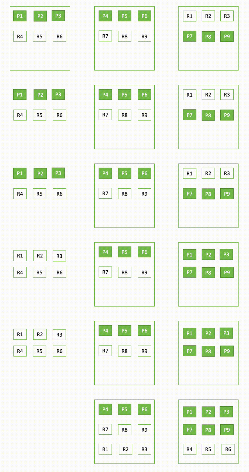
This behavior of the domain can be explained in two parts – during failure and during recovery.
During failure
A domain deployed across multiple Availability Zones can encounter multiple types of failures during its lifecycle.
Complete zone failure
A cluster may lose a single Availability Zone due to a variety of reasons and also all the nodes in that zone. Today, the service tries to place the lost nodes in the remaining healthy Availability Zones. The service also tries to re-create the lost shards in the remaining nodes while still following the allocation rules. This can result in some unintended consequences.
- When the shards of the impacted zone are getting reallocated to healthy zones, they trigger shard recoveries that can increase the latencies as it consumes additional CPU cycles and network bandwidth.
- For an n-AZ, n-copy setup, (n>1), the surviving n-1 Availability Zones are allocated with the nth shard copy, which can be undesirable as it can cause skewness in shard distribution, which can also result in unbalanced traffic across nodes. These nodes can get overloaded, leading to further failures.
Partial zone failure
In the event of a partial zone failure or when the domain loses only some of the nodes in an Availability Zone, Amazon OpenSearch Service tries to replace the failed nodes as quickly as possible. However, in case it takes too long to replace the nodes, OpenSearch tries to allocate the unassigned shards of that zone into the surviving nodes in the Availability Zone. If the service cannot replace the nodes in the impacted Availability Zone, it may allocate them in the other configured Availability Zone, which may further skew the distribution of shards both across and within the zone. This again has unintended consequences.
- If the nodes on the domain do not have enough storage space to accommodate the additional shards, the domain can be write-blocked, impacting indexing operation.
- Due to the skewed distribution of shards, the domain may also experience skewed traffic across the nodes, which can further increase the latencies or timeouts for read and write operations.
Recovery
Today, in order to maintain the desired node count of the domain, Amazon OpenSearch Service launches data nodes in the remaining healthy Availability Zones, similar to the scenarios described in the failure section above. In order to ensure proper node distribution across all the Availability Zones after such an incident, manual intervention was needed by AWS.
What’s changing
To improve the overall failure handling and minimizing the impact of failure on the domain health and performance, Amazon OpenSearch Service is performing the following changes:
- Forced Zone Awareness: OpenSearch has a preexisting shard balancing configuration called forced awareness that is used to set the Availability Zones to which shards need to be allocated. For example, if you have an awareness attribute called zone and configure nodes in
zone1andzone2, you can use forced awareness to prevent OpenSearch from allocating replicas if only one zone is available:
With this example configuration, if you start two nodes with node.attr.zone set to zone1 and create an index with five shards and one replica, OpenSearch creates the index and allocates the five primary shards but no replicas. Replicas are only allocated once nodes with node.attr.zone set to zone2 are available.
Amazon OpenSearch Service will use the forced awareness configuration on Multi-AZ domains to ensure that shards are only allocated according to the rules of zone awareness. This would prevent the sudden increase in load on the nodes of the healthy Availability Zones.
- Load-Aware Shard Allocation: Amazon OpenSearch Service will take into consideration factors like the provisioned capacity, actual capacity, and total shard copies to calculate if any node is overloaded with more shards based on expected average shards per node. It would prevent shard assignment when any node has allocated a shard count that goes beyond this limit.
Note that any unassigned primary copy would still be allowed on the overloaded node to prevent the cluster from any imminent data loss.
Similarly, to address the manual recovery issue (as described in the Recovery section above), Amazon OpenSearch Service is also making changes to its internal scaling component. With the newer changes in place, Amazon OpenSearch Service will not launch nodes in the remaining Availability Zones even when it goes through the previously described failure scenario.
Visualizing the current and new behavior
For example, an Amazon OpenSearch Service domain is configured with 3-AZ, 6 data nodes, 12 primary shards, and 24 replica shards. The domain is provisioned across AZ-1, AZ-2, and AZ-3, with two nodes in each of the zones.
Current shard allocation:
Total number of shards: 12 Primary + 24 Replica = 36 shards
Number of Availability Zones: 3
Number of shards per zone (zone awareness is true): 36/3 = 12
Number of nodes per Availability Zone: 2
Number of shards per node: 12/2 = 6
The following diagram provides a visual representation of the domain setup. The circles denote the count of shards allocated to the node. Amazon OpenSearch Service will allocate six shards per node.

During a partial zone failure, where one node in AZ-3 fails, the failed node is assigned to the remaining zone, and the shards in the zone are redistributed based on the available nodes. After the changes described above, the cluster will not create a new node or redistribute shards after the failure of the node.
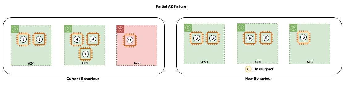
In the diagram above, with the loss of one node in AZ-3, Amazon OpenSearch Service would try to launch the replacement capacity in the same zone. However, due to some outage, the zone might be impaired and would fail to launch the replacement. In such an event, the service tries to launch deficit capacity in another healthy zone, which might lead to zone imbalance across Availability Zones. Shards on the impacted zone get stuffed on the surviving node in the same zone. However, with the new behavior, the service would try to attempt launching capacity in the same zone but would avoid launching deficit capacity in other zones to avoid imbalance. The shard allocator would also ensure that the surviving nodes don’t get overloaded.
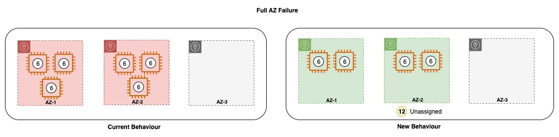
Similarly, in case all the nodes in AZ-3 are lost, or the AZ-3 becomes impaired, Amazon OpenSearch Service brings up the lost nodes in the remaining Availability Zone and also redistributes the shards on the nodes. However, after the new changes, Amazon OpenSearch Service will neither allocate nodes to the remaining zone or it will try to re-allocate lost shards to the remaining zone. Amazon OpenSearch Service will wait for the Recovery to happen and for the domain to return to the original configuration after recovery.
If your domain is not provisioned with enough capacity to withstand the loss of an Availability Zone, you may experience a drop in throughput for your domain. It is therefore strongly recommended to follow the best practices while sizing your domain, which means having enough resources provisioned to withstand the loss of a single Availability Zone failure.

Currently, once the domain recovers, the service requires manual intervention to balance capacity across Availability Zones, which also involves shard movements. However, with the new behaviour, there is no intervention needed during the recovery process because the capacity returns in the impacted zone and the shards are also automatically allocated to the recovered nodes. This ensures that there are no competing priorities on the remaining resources.
What you can expect
After you update your Amazon OpenSearch Service domain to the latest service software release, the domains that have been configured with best practices will have more predictable performance even after losing one or many data nodes in an Availability Zone. There will be reduced cases of shard overallocation in a node. It is a good practice to provision sufficient capacity to be able to tolerate a single zone failure
You might at times see a domain turning yellow during such unexpected failures since we won’t assign replica shards to overloaded nodes. However, this does not mean that there will be data loss in a well-configured domain. We will still make sure that all primaries are assigned during the outages. There is an automated recovery in place, which will take care of balancing the nodes in the domain and ensuring that the replicas are assigned once the failure recovers.
Update the service software of your Amazon OpenSearch Service domain to get these new changes applied to your domain. More details on the service software update process are in the Amazon OpenSearch Service documentation.
Conclusion
In this post we saw how Amazon OpenSearch Service recently improved the logic to distribute nodes and shards across Availability Zones during zonal outages.
This change will help the service to ensure more consistent and predictable performance during node or zonal failures. Domains won’t see any increased latencies or write blocks during processing writes and reads, which used to surface earlier at times due to over-allocation of shards on nodes.
About the authors
Bukhtawar Khan is a Senior Software Engineer working on Amazon OpenSearch Service. He is interested in distributed and autonomous systems. He is an active contributor to OpenSearch.
 Anshu Agarwal is a Senior Software Engineer working on AWS OpenSearch at Amazon Web Services. She is passionate about solving problems related to building scalable and highly reliable systems.
 Shourya Dutta Biswas is a Software Engineer working on AWS OpenSearch at Amazon Web Services. He is passionate about building highly resilient distributed systems.
 Rishab Nahata is a Software Engineer working on OpenSearch at Amazon Web Services. He is fascinated about solving problems in distributed systems. He is active contributor to OpenSearch.
This is a guest post by Vasily Ulianko and Per Brandser from Visma InSchool.
Located in Europe and Latin America, with headquarters in Norway, Visma has a bold vision to shape the future of society through technology. To do that, we provide business-critical software solutions for over 1 million customers across the Nordics, Benelux, Central and Eastern Europe, and Latin America. We are most interested in solving business problems with cutting-edge technology. We specialize in serverless technologies, optimization techniques, and data analytics, primarily focusing on building solutions for accounting, invoicing, procurement, and school administration.
Our solutions help simplify and streamline administrative tasks. From resource management, admissions, and documentation to financial management and generating diplomas, municipalities, and counties depend on the solutions Visma provides to make their schools run more efficiently.
Digitizing school operations is one of our most important social missions. Our goal is to contribute to making everyday work easier for school administrators and staff. Our flagship product for school administration, Visma InSchool, is a comprehensive system used by students, teachers, parents and administrators, for everything from planning school timetables to issuing diplomas. To make all information available anywhere, and at any time, through a single log in, we have built Visma InSchool to be a holistic system that lives in the cloud. Visma InSchool team uses Amazon QuickSight for business intelligence (BI) needs. `
The path to QuickSight
When we first started considering BI tools, a different solution was available to us through our company’s parent organization. That option, however, was two times more expensive per writer account, was harder to send the data to, and had a clunky and outdated user interface. Worse still, the amount of data that could be stored was also subject to external constraints.
The number of drawbacks with that solution would be more of a hindrance than an aid. We prioritize innovation, agility, and flexibility. We wanted to be in full control of the data source connections, user privileges, and data storage constraints. Researching other tools and what they offered that matched our requirements led us to QuickSight.
We started small, piloting QuickSight first with our product development teams, giving them the user experience they’d need to answer questions about our data from product and business owners. Due to the power of visualizing key actionable data, it didn’t take long before QuickSight was adopted and embraced by other departments.
Complex plans with simple solutions
One of the more difficult challenges for school administrators is developing plans for the upcoming school year. Not only do lesson plans need to be made for each class, but it’s crucial for administrators to have an early understanding of how many teachers will be available in comparison to what the school’s needs are and what those numbers mean in terms of financial impact. Through Personnel Planning functionality, Visma InSchool helps each school identify any discrepancies between existing teaching staff and what’s needed, which helps plan for both the recruitment and redundancy process.

We present school administrators with an automated timetable optimization view, offering extensive editing capabilities via Visma InSchool.

School administrators can now create well-organized lesson schedules that take into account the number of teachers, room availability, required teaching hours, and more.
The schools have to plan the lessons to cover the required hours for each subject in accordance with each individual student’s education program. QuickSight allows us to aggregate the data from this planning process, providing us with a high-level overview that offers the ability to drill down to the county and school levels. This gives our product and consulting teams the tools necessary to guide customers through their school-year planning process.

Automation saves time for school administrators and staff
When we initially started looking at QuickSight, our original intention was simply to use it for visualizations related to Visma InSchool product usage. The more we learned about its capabilities, however, the more we discovered other ways where QuickSight could deliver value. QuickSight has helped us streamline and automate several processes that have not only improved efficiency but saved our customers time and money as well.

Based on the data collected during this experiment, our consultants were able to advocate for the use of automated workflows among users. Not only did automation save time for school administrators and their staff, but it also helped product developers measure how useful it would be to research and develop new opportunities for automation.
One solution for all our needs
Different teams have different challenges, and there are often different approaches to solving them. One of the things that we love about QuickSight is its flexibility, which allows us to customize whatever we need based on each team’s specific priorities.
This is a brief overview of how our teams and our customers are using QuickSight every day:
- Product management – Our product management team uses QuickSight to track and measure key metrics, such as the number of timetables being published, the number of salary records created, and whether formative assessments are being created. Having these key metrics on hand, the product management team can experiment with hypotheses that help them improve the product, moving it in the right direction for what will be most helpful to our customers.

- Support – To help with critical warnings, our support consultants use QuickSight dashboards, which are updated hourly to proactively contact customers and escalate the problem to the relevant team before a customer submits a support ticket.
- Consulting – Our consulting teams use the data to tailor their consulting services and inform their training sessions and workshops with school administrators.
- Engineering – Our engineering teams use QuickSight to receive production error reports, allowing them to visualize usage statistics as well as discrepancies among different but related datasets.

- Customers – Our customers are most interested in the user base and sign-in statistics, as well as key results of school work, e.g., statistics on issued diplomas at the end of the academic year.
Yet another reason why we love QuickSight is how simple and seamless it is to integrate with our existing architecture. We are using a set of Amazon Aurora databases that back our system microservices, housing around 4 TB of data in more than 1,000 tables. With so much that can go wrong with integrating systems, not having to worry about any of that with our QuickSight implementation was a major plus. Simple setup and a flexible, usage-based pricing model made QuickSight the best choice for us.
QuickSight for dashboards and reports is just the beginning
We’ve had QuickSight for about 3 years now and have no regrets. Having been built by Amazon and accessible via the cloud, we rest easy knowing that it will continue to evolve and improve. Not having to worry about upgrades or maintenance is another upside to QuickSight; there have been several releases with new features and capabilities since we’ve been customers, and each one has brought an improved user experience.
In the future, we are planning to use Amazon QuickSight Embedded to deliver targeted BI information, interactive dashboards, and customized data visuals directly to our customers via Visma InSchool. As Norwegian counties manage their schools, they want insights and statistics across the schools in their county, which we can embed in their UI. Schools want information about their data and about teachers and students to make better decisions on adjustments and strategy. Empowering our customers with near-real-time information to make data-driven decisions is our goal, and we’re confident we can achieve it with QuickSight.
About the Authors
 Vasily Ulianko is a Director of Engineering in Visma InSchool, leading the development and operations, focusing on building strong engineering culture and solid system design.
 Per Brandser is a Product Strategy Manager in Visma InSchool. Mainly focusing on coaching our Product Managers on vision, product strategy and product discovery methodology, Per is a promoter of data driven product management.
This is a guest post from Tomotaka Inoue, Data Analyst at Leverages.
Founded in 2005, Leverages offers job staffing and web tools—Levtech and Levwell—for the IT and healthcare industries, serving both companies seeking talent and job seekers who are in the market for their next role. Inspired by a data point showing a proportional correlation between productivity and job change frequency, the company saw an opportunity to combine that insight with its passion for improving work environments for engineers. Providing a platform that enables skilled workers to easily find and pursue new opportunities meant a win-win for workers and companies alike.
The Levtech platform is a job search engine designed to not only effectively match companies with IT talent but also helps engineers and developers manage contracts, ensuring documentation is centralized for easy access. Levtech’s specialization for engineer and developer audiences has made it a hit within the IT freelance market.
Driving valuable and effective engagement with customers
One of the more challenging aspects of meeting customer needs within a human resources capacity comes in appropriately balancing priorities without the risk of missing opportunities for valuable engagement. On the higher-touch end of the spectrum, users who are actively engaged to both recruit and pursue open roles are necessarily high on the priority list. We want them to have a great experience and to be happy with the end result when the role is filled. But how do we maintain a less intrusive but still valuable level of engagement with users who are registered on the platform but are not actively recruiting or seeking right now?
To make those lower-touch engagements valuable and effective, Leverages wanted to provide Levtech users with access to market trend data related to their areas of expertise. By providing this data via a dashboard that’s embedded directly into Levtech, not only do we provide valuable information to registered users, but doing so also enables recruiters to become more valuable partners when not-currently-active job seekers become active. By having access to market trend data, recommendations can be made, e.g., “The demand for skill X is increasing. Therefore, by acquiring this skill, more companies would be interested in you.” When determining which business intelligence platform would best serve our needs to provide this data to our Levtech users, we turned to Amazon QuickSight.
In this post, we discuss what influenced our decision to implement QuickSight Embedded, as well as some of the benefits we’ve seen since then.
Finding the right embedded analytics solution
The only constant in technology is that things are always changing. As job seekers, engineers and developers often have little data to keep a pulse on which skills and experiences are in the highest demand. For recruiters, it’s challenging to gain visibility into how large or small the talent pool is for candidates who possess those in-demand skills or have had extensive experience in certain areas. Answering questions like these was the primary motivation for choosing QuickSight to help bring expanded functionality and increased value to Levtech.
When determining what our new business intelligence solution needed to have, we had three top priorities.
- Rich embedding features. Anonymous embedding was a key differentiator for us, enabling us to quickly launch because there were no user management or single sign-on (SSO) requirements.
- Easy to use. Analysis tools are useless if they’re not intuitive and user-friendly. With QuickSight, we were able to create beautiful dashboards very quickly.
- Cost-effective. Because QuickSight is serverless and offers session-based, on-demand pricing, it was a perfect fit for our budget.
One of our favorite things about QuickSight is that nondevelopers can update visuals on a dashboard. We often get requests from users that they want to see data from different angles, using a variety of charts. With other tools, making adjustments like that would require development resources with deep coding expertise to ensure the implementation was done correctly. With QuickSight, users of all technical ability levels can make updates without needing to rely on development resources.
The following screenshot shows an example of one of our dashboards.

Demystifying business decisions with data
In today’s world of lightning-fast communication, it’s more important than ever to be vigilant in using data to drive decisions. For the IT freelance community—both companies and job seekers—having immediate access to the data they need to make sound decisions is invaluable. For the companies we serve, dashboards can be built to show summaries of registered engineers within our database, their salary ranges, skill trends, how many job seekers there are, and more. Engineers and developers can access dashboards showing summaries of available positions, the number of freelance positions, skill requirements, etc.
For Leverages, QuickSight is helping to improve our sales and marketing efficiency because the QuickSight Embedded SDK helps reduce the time it takes to gather insights. We can now filter the actions Levtech users are making to discover data points, e.g., more companies are searching for Java engineers. Those insights can help inform not only talent suggestions but marketing campaigns as well.
Fast, efficient, intuitive embedded analytics in two days
By embedding QuickSight into Levtech, we have been able to offer thousands of users a fast, efficient, intuitive experience in accessing the data they need to make key decisions about their companies and their careers. Not only is QuickSight easy to use, implementation is exceptionally fast. Other tools we considered quoted us several months to get up and running, whereas our QuickSight implementation was done in just two business days.
To learn more about how you can embed customized data visuals, interactive dashboards, and natural language querying into any application, visit Amazon QuickSight Embedded.
About the Author
 Tomotaka Inoue is a data analyst at Leverages. Tomotaka analyzes Levtech’s data and suggests about the strategy and marketing.
Amazon Virtual Private Cloud (Amazon VPC) flow logs enable you to track the IP traffic going to and from the network interfaces in your VPC for your workloads. Analyzing VPC logs helps you understand how your applications are communicating over your VPC network with log records and acts as a main source of information to the network in your VPC. After collecting the flow logs, the next step is performing log analysis to understand user or application behavior and patterns to make informed decisions. You can analyze logs using log analytics tools such as Amazon OpenSearch Service.
Amazon Kinesis Data Firehose is a fully managed service for delivering near real-time streaming data to various destinations for storage and performing near real-time analytics. With its extensible data transformation capabilities, you can also streamline log processing and log delivery pipelines into a single Firehose delivery stream.
Amazon OpenSearch Service makes it easy for you to perform interactive log analytics, real-time application monitoring, website search, and more. Amazon OpenSearch is an open source, distributed search and analytics suite. Amazon OpenSearch Service offers the latest versions of OpenSearch, support for 19 versions of Elasticsearch (1.5 to 7.10 versions), as well as visualization capabilities powered by OpenSearch Dashboards and Kibana (1.5 to 7.10 versions). Amazon OpenSearch Service currently has tens of thousands of active customers with hundreds of thousands of clusters under management processing trillions of requests per month.
In this post, you will learn how to ingest VPC flow logs with Kinesis Data Firehose and deliver them to an Amazon OpenSearch Service for analysis using OpenSearch Service Dashboards.
Overview of solution
This solution uses native integration of VPC flow logs streaming to Kinesis Data Firehose. We use a Firehose delivery stream to buffer the streamed VPC flow logs, and deliver those to an OpenSearch Service destination endpoint. We use Amazon OpenSearch Service Dashboards to create an index pattern for the VPC flow logs to analyze and visualize the logs in a near-real time. The following diagram illustrates this architecture.

We walk you through the following high-level steps:
- Create an OpenSearch Service domain for storing and analyzing the VPC flow logs.
- Create a Firehose delivery stream to deliver the flow logs to the OpenSearch Service domain.
- Create a VPC flow log subscription to the delivery stream.
- Explore VPC flow logs in OpenSearch Service Dashboards
- Create role mapping with an OpenSearch Service user to the Kinesis Data Firehose service role. Because we’re using a public access domain for OpenSearch Service, we have to map the delivery stream AWS Identity and Access Management (IAM) role to the OpenSearch Service primary user to deliver logs in bulk to the OpenSearch Service domain.
- Create an index pattern in OpenSearch Service Dashboards to enable analysis and visualization of VPC logs.
Prerequisites
As a prerequisite, you need to create an Amazon Simple Storage Service (Amazon S3) bucket to store the Firehose delivery stream backups and failed logs.
Create an Amazon OpenSearch Service domain
For demonstration purposes, and to limit the costs, we create an OpenSearch Service domain with the Development and testing deployment type and public access to the dashboard. For instructions, refer to Create an Amazon OpenSearch Service domain. Note that we select Public access only for demo purposes. For production, we recommend using VPC access for security reasons.
When it’s complete, the OpenSearch Service domain shows as Active.

Create a Kinesis Data Firehose delivery stream
Now that your Amazon OpenSearch Service domain is active, you can create a Firehose delivery stream where VPC flow logs are streamed.
- On the Amazon Kinesis console, choose Kinesis Data Firehose in the navigation pane, then choose Create delivery stream.
- Choose Direct PUT as the source and set the destination as Amazon OpenSearch Service.
- For Delivery stream name, enter
PUT-OPENSEARCH-STREAM-DEMO.
- In the Destination settings section, choose Browse and choose the previously created Amazon OpenSearch Service domain.
- For Index name, enter vpcflowlogs.
- For Index rotation, choose Every day.
- For this post, we set Buffer size to 5 and Buffer interval to 900.You can modify these settings to optimize ingestion throughput and near-real-time behavior.

- In the Backup settings section, for Source record backup in Amazon S3, select Failed events only so you only save the data that fails to deliver to Amazon OpenSearch Service.
- For S3 bucket, choose Browse and choose the S3 bucket you created to store failed logs and backups.
- Optionally, you can input a prefix for backup files and error files.
- Select GZIP for Compression for data records.
- For Encryption for data records, select Disabled.

- Expand Advanced settings, and for Amazon CloudWatch error logging, select Enabled.
- Choose Create delivery stream.

When the delivery stream is active, proceed to the next step.
Create a VPC flow logs subscription
Now you create a VPC flow logs subscription for the Firehose delivery stream you created in the previous step.
- On the Amazon VPC console, choose Your VPCs.
- Select the VPC for which to create the flow log.
- On the Actions menu, choose Create flow log.
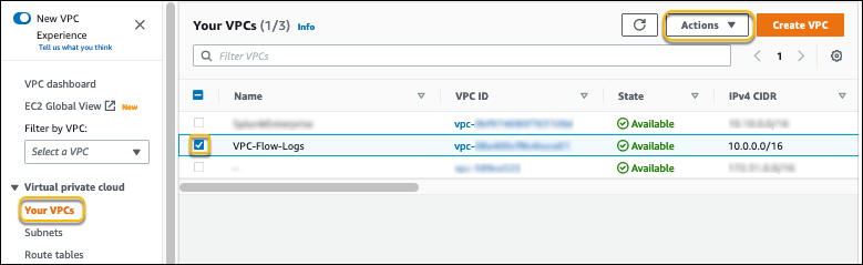
- Select All to send all flow log records to Amazon OpenSearch Service.
If you want to filter the flow logs, you can select either Accept or Reject.
- For Maximum aggregation interval, select 10 minutes or the minimum setting of 1 minute if you need the flow log data to be available for near-real-time analysis in Amazon OpenSearch Service.
- For Destination, select Send to Kinesis Firehose in the same account if the delivery stream is set up on the same account where you create the VPC flow logs.
- For Log record format, if you leave it at AWS default format, the flow logs are sent as version 2 format.
Alternatively, you can specify which fields you need the flow logs to capture and send to an Amazon OpenSearch Service. For more information on log format and available fields, refer to Flow log records.
- Choose Create flow log.
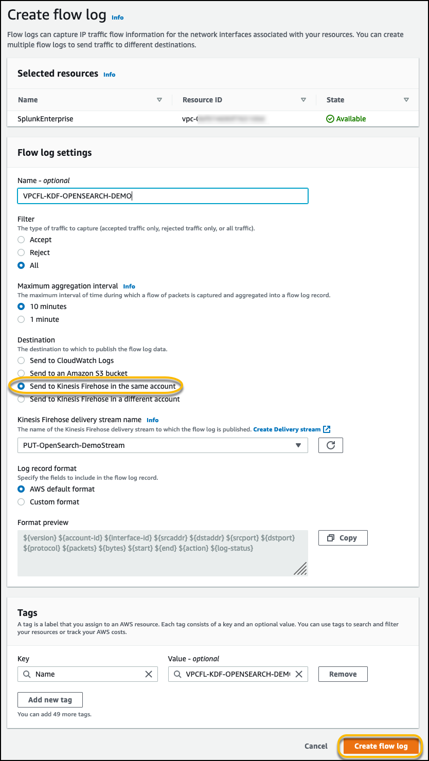
Now let’s explore the VPC flow logs in Amazon OpenSearch Service.
Explore VPC flow logs in Amazon OpenSearch Service Dashboards
In the final step, we set up OpenSearch Service Dashboards to explore the VPC flow logs.
- On the OpenSearch Service console, choose Domains in the navigation pane.
- Choose the domain you created.
- Under OpenSearch Dashboards URL, choose the link to open a new tab.

- Log in with the user you created during OpenSearch Service domain setup.

- Select Private for Select your tenant, then choose Confirm.

Because we used a public access domain for OpenSearch Service, you need to map the role created for the Firehose delivery stream to the OpenSearch Service Dashboards user, so that the delivery stream can deliver logs in bulk to the OpenSearch Service domain.
- On the menu icon, choose Security.
- Choose Roles.
- Choose the
all\_accessrole.
- On the Mapped users tab, choose Manage mapping.

- For Backend roles, enter the IAM role ARN created for the Firehose delivery stream.
- Choose Map.

- Now that mapping is complete, choose the menu icon, then choose Stack management.

- Choose Index Patterns, then choose Create index pattern.
- For Index pattern name, enter
vpcflowlogs*. - Choose Next step.

- Navigate to the Discover menu option.You can see the VPC flow logs from your VPC in this dashboard. Now you can search and visualize the flow logs that are being streamed in near-real time to the OpenSearch Service domain.

Clean up
After you test out this solution, remember to delete all the resources you created to avoid incurring future charges:
- Delete your Amazon OpenSearch Service domain.
- Delete the VPC flow logs subscription.
- Delete the Firehose delivery stream.
- Delete the S3 bucket for the VPC flow logs backup and failed logs.
- If you created a new VPC and new resources in the VPC, delete the resources and VPC.
Conclusion
In this post, we walked through a solution of how integrate VPC flow logs with a Kinesis Data Firehose delivery stream and deliver it to an Amazon OpenSearch Service destination with no code and visualize it in OpenSearch Service Dashboards.
Try this new quick and hassle-free way of sending your VPC flow logs to an Amazon OpenSearch Service using Kinesis Data Firehose.
About the Author
 Chaitanya Shah is a Sr. Technical Account Manager with AWS, based out of New York. He has over 22 years of experience working with enterprise customers. He loves to code and actively contributes to the AWS solutions labs to help customers solve complex problems. He provides guidance to AWS customers on best practices for their AWS Cloud migrations. He is also specialized in AWS data transfer and the data and analytics domain.
Amazon Redshift is a fast, scalable, secure, and fully-managed data warehouse that enables you to analyze all of your data using standard SQL easily and cost-effectively. Amazon Redshift Data Sharing allows customers to securely share live, transactionally consistent data in one Amazon Redshift cluster with another Amazon Redshift cluster across accounts and regions without needing to copy or move data from one cluster to another.
Amazon Redshift Data Sharing was initially launched in March 2021, and added support for cross-account data sharing was added in August 2021. The cross-region support became generally available in February 2022. This provides full flexibility and agility to share data across Redshift clusters in the same AWS account, different accounts, or different regions.
Amazon Redshift Data Sharing is used to fundamentally redefine Amazon Redshift deployment architectures into a hub-spoke, data mesh model to better meet performance SLAs, provide workload isolation, perform cross-group analytics, easily onboard new use cases, and most importantly do all of this without the complexity of data movement and data copies. Some of the most common questions asked during data sharing deployment are, “How big should my consumer clusters and producer clusters be?”, and “How do I get the best price performance for workload isolation?”. As workload characteristics like data size, ingestion rate, query pattern, and maintenance activities can impact data sharing performance, a continuous strategy to size both consumer and producer clusters to maximize the performance and minimize cost should be implemented. In this post, we provide a step-by-step approach to help you determine your producer and consumer clusters sizes for the best price performance based on your specific workload.
Generic consumer sizing guidance
The following steps show the generic strategy to size your producer and consumer clusters. You can use it as a starting point and modify accordingly to cater your specific use case scenario.
Size your producer cluster
You should always make sure that you properly size your producer cluster to get the performance that you need to meet your SLA. You can leverage the sizing calculator from the Amazon Redshift console to get a recommendation for the producer cluster based on the size of your data and query characteristic. Look for Help me choose on the console in AWS Regions that support RA3 node types to use this sizing calculator. Note that this is just an initial recommendation to get started, and you should test running your full workload on the initial size cluster and elastic resize the cluster up and down accordingly to get the best price performance.

Size and setup initial consumer cluster
You should always size your consumer cluster based on your compute needs. One way to get started is to follow the generic cluster sizing guide similar to the producer cluster above.
Setup Amazon Redshift data sharing
Setup data sharing from producer to consumer once you have both the producer and consumer cluster setup. Refer to this post for guidance on how to setup data sharing.
Test consumer only workload on initial consumer cluster
Test consumer only workload on the new initial consumer cluster. This can be done by pointing consumer applications, for example ETL tools, BI applications, and SQL clients, to the new consumer cluster and rerunning the workload to evaluate the performance against your requirements.
Test consumer only workload on different consumer cluster configurations
If the initial size consumer cluster meets or exceeds your workload performance requirements, then you can either continue to use this cluster configuration or you can test on smaller configurations to see if you can further reduce the cost and still get the performance that you need.
On the other hand, if the initial size consumer cluster fails to meet your workload performance requirements, then you can further test larger configurations to get the configuration that meets your SLA.
As a rule of thumb, size up the consumer cluster by 2x the initial cluster configuration incrementally until it meets your workload requirements.
Once you plan out what configuration you want to test, use elastic resize to resize the initial cluster to the target cluster configuration. After elastic resize is completed, perform the same workload test and evaluate the performance against your SLA. Select the configuration that meets your price performance target.
Test producer only workload on different producer cluster configurations
Once you move your consumer workload to the consumer cluster with the optimum price performance, there might be an opportunity to reduce the compute resource on the producer to save on costs.
To achieve this, you can rerun the producer only workload on 1/2x of the original producer size and evaluate the workload performance. Resizing the cluster up and down accordingly depends on the result, and then you select the minimum producer configuration that meets your workload performance requirements.
Re-evaluate after a full workload run over time
As Amazon Redshift continues evolving, and there are continuous performance and scalability improvement releases, data sharing performance will continue improving. Furthermore, numerous variables might impact the performance of data sharing queries. The following are just some examples:
- Ingestion rate and amount of data change
- Query pattern and characteristic
- Workload changes
- Concurrency
- Maintenance activities, for example vacuum, analyze, and ATO
This is why you must re-evaluate the producer and consumer cluster sizing using the strategy above on occasion, especially after a full workload deployment, to gain the new best price performance from your cluster’s configuration.
Automated sizing solutions
If your environment involved more complex architecture, for example with multiple tools or applications (BI, ingestion or streaming, ETL, data science), then it might not feasible to use the manual method from the generic guidance above. Instead, you can leverage solutions in this section to automatically replay the workload from your production cluster on the test consumer and producer clusters to evaluate the performance.
Simple Replay utility will be leveraged as the automated solution to guide you through the process of getting the right producer and consumer clusters size for the best price performance.
Simple Replay is a tool for conducting a what-if analysis and evaluating how your workload performs in different scenarios. For example, you can use the tool to benchmark your actual workload on a new instance type like RA3, evaluate a new feature, or assess different cluster configurations. It also includes enhanced support for replaying data ingestion and export pipelines with COPY and UNLOAD statements. To get started and replay your workloads, download the tool from the Amazon Redshift GitHub repository.
Here we walk through the steps to extract your workload logs from the source production cluster and replay them in an isolated environment. This lets you perform a direct comparison between these Amazon Redshift clusters seamlessly and select the clusters configuration that best meet your price performance target.
The following diagram shows the solution architecture.

Solution walkthrough
Follow these steps to go through the solution to size your consumer and producer clusters.
Size your production cluster
You should always make sure to properly size your existing production cluster to get the performance that you need to meet your workload requirements. You can leverage the sizing calculator from the Amazon Redshift console to get a recommendation on the production cluster based on the size of your data and query characteristic. Look for Help me choose on the console in AWS Regions that support RA3 node types to use this sizing calculator. Note that this is just an initial recommendation to get started. You should test running your full workload on the initial size cluster and elastic resize the cluster up and down accordingly to get the best price performance.
Identify the workload to be isolated
You might have different workloads running on your original cluster, but the first step is to identify the most critical workload to the business that we want to isolate. This is because we want to make sure that the new architecture can meet your workload requirements. This post is a good reference on a data sharing workload isolation use case that can help you decide which workload can be isolated.
Setup Simple Replay
Once you know your critical workload, you must enable audit logging in your production cluster where the critical workload identified above is running to capture query activities and store in Amazon Simple Storage Service (Amazon S3). Note that it may take up to three hours for the audit logs to be delivered to Amazon S3. Once the audit log is available, proceed to setup Simple Replay and then extract the critical workload from the audit log. Note that start\_time and end\_time could be used as parameters to filter out the critical workload if those workloads run in certain time periods, for example 9am to 11am. Otherwise it will extract all of the logged activities.
Baseline workload
Create a baseline cluster with the same configuration as the producer cluster by restoring from the production snapshot. The purpose of starting with the same configuration is to baseline the performance with an isolated environment.
Once the baseline cluster is available, replay the extracted workload in the baseline cluster. The output from this replay will be the baseline used to compare against subsequent replays on different consumer configurations.
Setup initial producer and consumer test clusters
Create a producer cluster with the same production cluster configuration by restoring from the production snapshot. Create a consumer cluster with the recommended initial consumer size from the previous guidance. Furthermore, setup data sharing between the producer and consumer.
Replay workload on initial producer and consumer
Replay the producer only workload on the initial size producer cluster. This can be achieved using the “Exclude” filter parameter to exclude consumer queries, for example the user that runs consumer queries.
Replay the consumer only workload on the initial size consumer cluster. This can be achieved using the “Include” filter parameter to exclude consumer queries, for example the user that runs consumer queries.
Evaluate the performance of these replays against the baseline and workload performance requirements.
Replay consumer workload on different configurations
If the initial size consumer cluster meets or exceeds your workload performance requirements, then you can either use this cluster configuration or you can follow these steps to test on smaller configurations to see if you can further reduce costs and still get the performance that you need.
Compare initial consumer performance results against your workload requirements:
- If the result exceeds your workload performance requirements, then you can reduce the size of the consumer cluster incrementally, starting with 1/2x, retry the replay and evaluate the performance, then resize up or down accordingly based on the result until it meets your workload requirements. The purpose is to get a sweet spot where you’re comfortable with the performance requirements and get the lowest price possible.
- If the result fails to meet your workload performance requirements, then you can increase the size of the cluster incrementally, starting with 2x the original size, retry the replay and evaluate the performance until it meets your workload performance requirements.
Replay producer workload on different configurations
Once you split your workloads out to consumer clusters, the load on the producer cluster should be reduced and you should evaluate your producer cluster’s workload performance to seek the opportunity to downsize to save on costs.
The steps are similar to consumer replay. Elastic resize the producer cluster incrementally starting with 1/2x the original size, replay the producer only workload and evaluate the performance, and then further resize up or down until it meets your workload performance requirements. The purpose is to get a sweet spot where you’re comfortable with the workload performance requirements and get the lowest price possible. Once you have the desired producer cluster configuration, retry replay consumer workloads on the consumer cluster to make sure that the performance wasn’t impacted by producer cluster configuration changes. Finally, you should replay both producer and consumer workloads concurrently to make sure that the performance is achieved in a full workload scenario.
Re-evaluate after a full workload run over time
Similar to the generic guidance, you should re-evaluate the producer and consumer clusters sizing using the previous strategy on occasion, especially after full workload deployment to gain the new best price performance from your cluster’s configuration.
Clean up
Running these sizing tests in your AWS account may have some cost implications because it provisions new Amazon Redshift clusters, which may be charged as on-demand instances if you don’t have Reserved Instances. When you complete your evaluations, we recommend deleting the Amazon Redshift clusters to save on costs. We also recommend pausing your clusters when they’re not in use.
Applying Amazon Redshift and data sharing best practices
Proper sizing of both your producer and consumer clusters will give you a good start to get the best price performance from your Amazon Redshift deployment. However, sizing isn’t the only factor that can maximize your performance. In this case, understanding and following best practices are equally important.
General Amazon Redshift performance tuning best practices are applicable to data sharing deployment. Make sure that your deployment follows these best practices.
There numerous data sharing specific best practices that you should follow to make sure that you maximize the performance. Refer to this post for more details.
Summary
There is no one-size-fits-all recommendation on producer and consumer cluster sizes. It varies by workloads and your performance SLA. The purpose of this post is to provide you with guidance for how you can evaluate your specific data sharing workload performance to determine both consumer and producer cluster sizes to get the best price performance. Consider testing your workloads on producer and consumer using simple replay before adopting it in production to get the best price performance.
About the Authors
 BP Yau is a Sr Product Manager at AWS. He is passionate about helping customers architect big data solutions to process data at scale. Before AWS, he helped Amazon.com Supply Chain Optimization Technologies migrate its Oracle data warehouse to Amazon Redshift and build its next generation big data analytics platform using AWS technologies.
 Sidhanth Muralidhar is a Principal Technical Account Manager at AWS. He works with large enterprise customers who run their workloads on AWS. He is passionate about working with customers and helping them architect workloads for costs, reliability, performance and operational excellence at scale in their cloud journey. He has a keen interest in Data Analytics as well.
Amazon EMR on EKS is a deployment option in Amazon EMR that allows you to run Spark jobs on Amazon Elastic Kubernetes Service (Amazon EKS). Amazon Elastic Compute Cloud (Amazon EC2) Spot Instances save you up to 90% over On-Demand Instances, and is a great way to cost optimize the Spark workloads running on Amazon EMR on EKS. Because Spot is an interruptible service, if we can move or reuse the intermediate shuffle files, it improves the overall stability and SLA of the job. The latest versions of Amazon EMR on EKS have integrated Spark features to enable this capability.
In this post, we discuss these features—Node Decommissioning and Persistent Volume Claim (PVC) reuse—and their impact on increasing the fault tolerance of Spark jobs on Amazon EMR on EKS when cost optimizing using EC2 Spot Instances.
Amazon EMR on EKS and Spot
EC2 Spot Instances are spare EC2 capacity provided at a steep discount of up to 90% over On-Demand prices. Spot Instances are a great choice for stateless and flexible workloads. The caveat with this discount and spare capacity is that Amazon EC2 can interrupt an instance with a proactive or reactive (2-minute) warning when it needs the capacity back. You can provision compute capacity in an EKS cluster using Spot Instances using a managed or self-managed node group and provide cost optimization for your workloads.
Amazon EMR on EKS uses Amazon EKS to run jobs with the EMR runtime for Apache Spark, which can be cost optimized by running the Spark executors on Spot. It provides up to 61% lower costs and up to 68% performance improvement for Spark workloads on Amazon EKS. The Spark application launches a driver and executors to run the computation. Spark is a semi-fault tolerant framework that is resilient to executor loss due to an interruption and therefore can run on EC2 Spot. On the other hand, when the driver is interrupted, the job fails. Hence, we recommend running drivers on on-demand instances. Some of the best practices for running Spark on Amazon EKS are applicable with Amazon EMR on EKS.
EC2 Spot instances also helps in cost optimization by improving the overall throughput of the job. This can be achieved by auto-scaling the cluster using Cluster Autoscaler (for managed nodegroups) or Karpenter.
Though Spark executors are resilient to Spot interruptions, the shuffle files and RDD data is lost when the executor gets killed. The lost shuffle files need to be recomputed, which increases the overall runtime of the job. Apache Spark has released two features (in versions 3.1 and 3.2) that addresses this issue. Amazon EMR on EKS released features such as node decommissioning (version 6.3) and PVC reuse (version 6.8) to simplify recovery and reuse shuffle files, which increases the overall resiliency of your application.
Node decommissioning
The node decommissioning feature works by preventing scheduling of new jobs on the nodes that are to be decommissioned. It also moves any shuffle files or cache present in those nodes to other executors (peers). If there are no other available executors, the shuffle files and cache are moved to a remote fallback storage.

Fig 1 : Node Decommissioning
Let’s look at the decommission steps in more detail.
If one of the nodes that is running executors is interrupted, the executor starts the process of decommissioning and sends the message to the driver:
The executor looks for RDD or shuffle files and tries to replicate or migrate those files. It first tries to find a peer executor. If successful, it will move the files to the peer executor:
However, if It is not able to find a peer executor, it will try to move the files to a fallback storage if available.

Fig 2: Fallback Storage
The executor is then decommissioned. When a new executor comes up, the shuffle files are reused:
The key advantage of this process is that it enables migrates blocks and shuffle data, thereby reducing recomputation, which adds to the overall resiliency of the system and reduces runtime. This process can be triggered by a Spot interruption signal (Sigterm) and node draining. Node draining may happen due to high-priority task scheduling or independently.
When you use Amazon EMR on EKS with managed node groups/Karpenter, the Spot interruption handling is automated, wherein Amazon EKS gracefully drains and rebalances the Spot nodes to minimize application disruption when a Spot node is at elevated risk of interruption. If you’re using managed node groups/Karpenter, the decommission gets triggered when the nodes are getting drained and because it’s proactive, it gives you more time (at least 2 minutes) to move the files. In the case of self-managed node groups, we recommend installing the AWS Node Termination Handler to handle the interruption, and the decommission is triggered when the reactive (2-minute) notification is received. We recommend to use Karpenter with Spot Instances as it has faster node scheduling with early pod binding and binpacking to optimize the resource utilization.
The following code enables this configuration; more details are available on GitHub:
PVC reuse
Apache Spark enabled dynamic PVC in version 3.1, which is useful with dynamic allocation because we don’t have to pre-create the claims or volumes for the executors and delete them after completion. PVC enables true decoupling of data and processing when we’re running Spark jobs on Kubernetes, because we can use it as a local storage to spill in-process files too. The latest version of Amazon EMR 6.8 has integrated the PVC reuse feature of Spark, wherein if an executor is terminated due to EC2 Spot interruption or any other reason (JVM), then the PVC is not deleted but persisted and reattached to another executor. If there are shuffle files in that volume, then they are reused.
As with node decommission, this reduces the overall runtime because we don’t have to recompute the shuffle files. We also save the time required to request a new volume for an executor, and shuffle files can be reused without moving the files round.
The following diagram illustrates this workflow.

Fig 3: PVC Reuse
Let’s look at the steps in more detail.
If one or more of the nodes that are running executors is interrupted, the underlying pods get terminated and the driver gets the update. Note that the driver is the owner of the PVC of the executors, and they are not terminated. See the following code:
The ExecutorPodsAllocator tries to allocate new executor pods to replace the ones terminated due to interruption. During the allocation, it figures out how many of the existing PVCs have files and can be reused:
The ExecutorPodsAllocator requests for a pod and when it launches it, the PVC is reused. In the following example, the PVC from executor 6 is reused for new executor pod 11:
The shuffle files, if present in the PVC are reused.
The key advantage of this technique is that it allows us to reuse pre-computed shuffle files in their original location, thereby reducing the time of the overall job run.
This works for both static and dynamic PVCs. Amazon EKS offers three different storage offerings, which can be encrypted too: Amazon Elastic Block Store (Amazon EBS), Amazon Elastic File System (Amazon EFS), and Amazon FSx for Lustre. We recommend using dynamic PVCs with Amazon EBS because with static PVCs, you would need to create multiple PVCs.
The following code enables this configuration; more details are available on GitHub:
For this to work, we need to enable PVC with Amazon EKS and mention the details in the Spark runtime configuration. For instructions, refer to How do I use persistent storage in Amazon EKS? The following code contains the Spark configuration details for using PVC as local storage; other details are available on GitHub:
Conclusion
With Amazon EMR on EKS (6.9) and the features discussed in this post, you can further reduce the overall runtime for Spark jobs when running with Spot Instances. This also improves the overall resiliency and flexibility of the job while cost optimizing the workload on EC2 Spot.
Try out the EMR on EKS workshop for improved performance when running Spark workloads on Kubernetes and cost optimize using EC2 Spot Instances.
About the Author
 Kinnar Kumar Sen is a Sr. Solutions Architect at Amazon Web Services (AWS) focusing on Flexible Compute. As a part of the EC2 Flexible Compute team, he works with customers to guide them to the most elastic and efficient compute options that are suitable for their workload running on AWS. Kinnar has more than 15 years of industry experience working in research, consultancy, engineering, and architecture.
Missed AWS re:Invent 2022? We’ve got you covered!
AWS offers the most scalable, highest performing data services to keep up with the growing volume and velocity of data to help organizations to be data-driven in real-time. We help customers unify diverse data sources by investing in a zero ETL future. We provide the industry’s most comprehensive set of capabilities for an end-to-end data strategy for all your workloads. And, our services help you enable end-to-end data governance so your teams are free to move faster with data.
This post walks you through all of the new analytics service launches. You’ll find links to blog posts, announcements, session recordings, and press releases so you can dive deeper into those launches.
For more 2022 re:Invent recaps and ongoing coverage of all the important AWS launches, be sure to stay in touch with us here:
- Analytics at re:Invent: session recordings
- AWS Databases & Analytics online events: Analytics in 15, fireside chat, deep dive, and roadmap
- Top announcements of AWS re:Invent 2022: AWS VP and Chief Evangelist Jeff Barr’s picks for some of the most impactful launches
Press releases
Press release – AWS Announces Five New Database and Analytics Capabilities
This press release covers five new database and analytics capabilities that make it faster and easier for you to manage and analyze data at petabyte scale—Amazon DocumentDB Elastic Clusters, Amazon OpenSearch Serverless, Amazon Athena for Apache Spark, AWS Glue Data Quality, and Amazon Redshift Multi-AZ.
Press release – AWS Announced Five New Capabilities for Amazon QuickSight
This press release covers five new capabilities for Amazon QuickSight, the most popular serverless BI service built for the cloud. These new capabilities will help customers streamline business intelligence operations.
Press release – AWS Announced Two New Capabilities to Move Toward a Zero-ETL Future on AWS
This press release covers two new integrations that make it easier for customers to connect and analyze data across data stores without having to move data between services.
Press release – AWS Announced Amazon DataZone
Amazon DataZone makes it faster and easier for customers to catalog, discover, share, and govern data stored across AWS, on premises, and on third-party sources. To learn more about Amazon DataZone, please visit the product page or watch the re:Invent session recording.
Keynotes and leadership sessions
Adam Selipsky, Chief Executive Officer of Amazon Web Services, highlighted innovations in data, infrastructure, and more that are helping customers achieve their goals faster, take advantage of untapped potential, and create a better future with AWS. The analytics new launches Adam mentioned include Amazon OpenSearch Serverless, Amazon DataZone, and Amazon Aurora zero-ETL integration with Amazon Redshift.
Swami Sivasubramanian, Vice President of AWS Data and Machine Learning, revealed the latest AWS innovations that can help you transform your company’s data into meaningful insights and actions for your business. In this keynote, Swami launched Amazon Athena for Apache Spark, Amazon Redshift integration for Apache Spark, Amazon Redshift Multi-AZ, AWS Glue Data Quality, and other new AWS capabilities.
G2 Krishnamoorthy, VP of AWS Analytics, covered the latest service innovations around data and also highlighted customer successes with AWS analytics. New analytics capabilities he covered include AWS Glue for Ray, Amazon Redshift Streaming Ingestion, Amazon Aurora zero-ETL to Amazon Redshift, Amazon Redshift integration for Apache Spark, Amazon DataZone, Amazon Athena for Apache Spark, Amazon OpenSearch Serverless, Amazon QuickSight API, and more.
Mai-Lan Tomsen Bukovec, Vice President of AWS Foundational Data Services, and Andy Warfield, AWS Distinguished Engineer, shared the latest AWS storage innovations and an inside look at how customers drive modern business on data lakes and with high-performance data. They also dived deep into technical and organizational strategies that protect with resilience, respond with agility, and fuel innovations with data-driven insights on AWS storage.
Amazon DataZone
To gain value from your data, it needs to be accessible by people and systems that need it for analytics. This session introduces you to Amazon DataZone, a new AWS business data catalog that allows you to unlock data across organizational boundaries with built-in governance.
Amazon Security Lake
- Blog – Preview: Amazon Security Lake – A Purpose-Built Customer-Owned Data Lake Service
This new service automatically centralizes your organization’s security data from cloud and on-premises sources into a purpose-built data lake stored in your account.
Amazon Redshift
- Blog – New for Amazon Redshift – Zero-ETL integration, simplified data ingestion techniques, security and reliability features.
This year at re:Invent, Amazon Redshift has announced a number of features to help you simplify data ingestion and get to insights easily and quickly within a secure, reliable environment. - Blog – New for Amazon Redshift – General Availability of Streaming Ingestion for Kinesis Data Streams and Managed Streaming for Apache Kafka
Amazon Redshift Streaming Ingestion ingests hundreds of megabytes of data per second so you can query data in near real time. You can connect to multiple Kinesis Data Streams or Amazon Managed Streaming for Apache Kafka data streams and pull data directly to Amazon Redshift without staging data in Amazon S3. - Blog – New – Amazon Redshift Integration with Apache Spark
This new release makes it easy to build and run Spark applications on Amazon Redshift and Redshift Serverless, enabling you to open up the data warehouse for a broader set of AWS analytics and machine learning (ML) solutions. - Blog – Simplify data ingestion from Amazon S3 to Amazon Redshift using auto-copy
This feature simplifies data loading from Amazon S3 into Amazon Redshift. You can now set up continuous file ingestion rules to track your Amazon S3 paths and automatically load new files without needing additional tools or custom solutions. - Blog – Centrally manage access and permissions for Amazon Redshift data sharing with AWS Lake Formation
This feature enables you to centrally manage access to your Amazon Redshift datashares using Lake Formation. It opens up new design patterns and broadens governance and security posture across data warehouses. - Blog – Simplify data loading on the Amazon Redshift console with Informatica Data Loader
You need to bring data quickly and at scale from various data stores. You also need a simple, easy, and cloud-native solution to quickly onboard new data sources or to analyze recent data for actionable insights. With this feature, you can securely connect and load data to Amazon Redshift at scale via a simple and guided interface.
Watch the recording to learn about important new features of Amazon Redshift. Learn how Amazon Redshift reinvented data warehousing to help you analyze all your data across data lakes, data warehouses, and databases with the best price performance. In this session, Goldman Sachs shared their Amazon Redshift use case.
Amazon OpenSearch Service
- Blog – Run Search and Analytics Workloads without Managing Clusters
This new release provisions and scales resources to deliver fast data ingestion and query responses for even the most demanding and unpredictable workloads, eliminating the need to configure and optimize clusters. Learn more by watching the recording of the re:Invent breakout session Provision & scale OpenSearch resources with serverless. To get started with Amazon OpenSearch Serverless, please join this workshop.
Streaming services
- Announcement – Introducing Amazon Managed Streaming for Apache Kafka (MSK) Delivery Partners
The new Amazon MSK Service Delivery specialization for AWS partners helps customers migrate and build real-time streaming analytics solutions with fully managed Apache Kafka. - Announcement – Amazon Kinesis Data Firehose adds support for data stream delivery to Amazon OpenSearch Serverless
With a few clicks, you can easily ingest, transform, and reliably deliver streaming data into an Amazon OpenSearch Serverless without building and managing your own data ingestion and delivery infrastructure.
AWS Glue
- Blog – Join the Preview – AWS Glue Data Quality
AWS Glue Data Quality can analyze your tables and recommend a set of rules automatically based on what it finds. - Announcement – Announcing AWS Glue for Ray (Preview)
Data engineers can use AWS Glue for Ray to process large datasets with Python and popular Python libraries. - Blog – New AWS Glue 4.0 – New and Updated Engines, More Data Formats, and More
This version of AWS Glue includes Python 3.10 and Apache Spark 3.3.0, plus native support for the Cloud Shuffle Storage Plugin for Apache Spark. It also includes Pandas support and more. - Announcement – Introducing AWS Glue Delivery
The new AWS Glue Delivery specialization validates AWS Partners with deep expertise and proven success in delivering AWS Glue for data integration, data pipeline, and data catalog use cases. - Announcement – AWS Glue for Apache Spark Native support for Data Lake Frameworks
AWS Glue for Apache Spark now supports three open-source data lake storage frameworks: Apache Hudi, Apache Iceberg, and Linux Foundation Delta Lake. - Announcement – AWS Glue introduces custom visual transforms
AWS Glue now offers custom visual transforms, which let customers define, reuse, and share business-specific ETL logic among their teams.
Amazon Athena
- Blog – New — Amazon Athena for Apache Spark
With this feature, we can run Apache Spark workloads, use Jupyter Notebook as the interface to perform data processing on Athena, and programmatically interact with Spark applications using Athena APIs.
Amazon QuickSight
- Blog – New analytical questions available in Amazon QuickSight Q: “Why” and “Forecast”
Amazon QuickSight announces support for two new question types that simplify and scale complex analytical tasks using natural language: “forecast” and “why.” - Blog – Announcing Automated Data Preparation for Amazon QuickSight Q
Automated data preparation uses machine learning to infer semantic information about data and adds it to datasets as metadata about the columns (fields), making it faster for you to prepare data in order to support natural language questions. - Blog – New Amazon QuickSight API Capabilities to Accelerate Your BI Transformation
New QuickSight API capabilities allow programmatic creation and management of dashboards, analysis, and templates. - Blog – Create and Share Operational Reports at Scale with Amazon QuickSight Paginated Reports
This feature allows customers to create and share highly formatted, personalized reports containing business-critical data to hundreds of thousands of end users—without any infrastructure setup or maintenance, up-front licensing, or long-term commitments.
Amazon AppFlow
- Blog – Announcing Additional Data Connectors for Amazon AppFlow
We’ve added 22 new data connectors for Amazon AppFlow, including connectors for marketing, customer service and engagement, and business operations.
Thanks for reading! re:Invent is certainly not just about new launches. The Analytics and Business Intelligence tracks dived deep into each one of the analytics services through sessions (86 in total!), covering a wide range of topics and use cases.
Check out the YouTube playlist for session recordings.
About the author
 Gwen Chen is Senior Product Marketing Manager for Amazon Redshift and re:Invent Analytics Track Lead. She believes in the power of communication, and likes data, analytics, and AI/ML.
Observability data provides near real-time insights into the health and performance of AWS workloads, so that engineers can quickly address production issues and troubleshoot them before widespread customer impact.
As AWS workloads grow, observability data has been exploding, which requires flexible big data solutions to handle the throughput of large and unpredictable volumes of observability data.
Solution overview
One option is Amazon Kinesis Data Firehose, which is a popular service for streaming huge volumes of AWS data for storage and analytics. By pulling data from Amazon CloudWatch, Amazon Kinesis Data Firehose can deliver data to observability solutions.
Among these observability solutions is Logz.io, which can now ingest metric data from Amazon Kinesis Data Firehose and make it easier to get metrics from your AWS account to your Logz.io account for analysis, alerting, and correlation with logs and traces.
In a few clicks and a few configurations, we’ll see how you can start streaming your metric data (and soon, log data!) to Logz.io for storage and analysis.
Prerequisites
- Logz.io account – Create a free trial here
- Logz.io shipping token – Learn about metrics tokens here. You need to be a Logz.io administrator.
- Access to Amazon CloudWatch and Amazon Kinesis Data Firehose with the appropriate permissions to manage HTTP endpoints.
- Appropriate permissions to create an Amazon Simple Storage Service (Amazon S3) bucket
Sending Amazon CloudWatch metric data to Logz.io with an Amazon Kinesis Data Firehose
Amazon Kinesis Data Firehose is a service for ingesting, processing, and loading data from large, distributed sources such as logs or clickstreams into multiple consumers for storage and real-time analytics. Kinesis Data Firehose supports more than 50 sources and destinations as of today. This integration can be set up in minutes without a single line of code and enables near real-time analytics for observability data generated by AWS services by using Amazon CloudWatch, Amazon Kinesis Data Firehose, and Logz.io.
Once the integration is configured, Logz.io customers can open the Infrastructure Monitoring product to see their data coming in and populating their dashboards. To see some of the data analytics and correlation you get with Logz.io, check out this short demonstration.
Let’s begin a step-by-step tutorial for setting up the integration.
- Start by going to Amazon Kinesis Data Firehose and creating a delivery stream with Data Firehose.

- Next you select a source and destination. Select Direct Put as the source and Logz.io the destination.
- Next, configure the destination settings. Give the HTTP endpoint a name, which should include logz.io.
- Select from the dropdown the appropriate endpoint you would like to use.
If you’re sending data to a European region, then set it to Logz.io Metrics EU. Or you can use the us-east-1 destination by selecting Logz.io Metrics US.
- Next, add your Logz.io Shipping Token. You can find this by going to Settings in Logz.io and selecting Manage Tokens, which requires Logz.io administrator to access. This ensures that your account is only ingesting data from the defined sources (e.g., this Amazon Kinesis Data Firehose delivery stream).
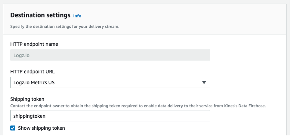
Keep Content encoding on Disabled and set your desired Retry Duration.
You can also configure Buffer hints to your preferences.
- Next, determine your Backup settings in case something goes wrong. In most cases, it’s only necessary to back up the failed data. Simply choose an Amazon S3 bucket or create a new one to store data if it doesn’t make it to Logz.io. Then, select Create a delivery stream.
Now it’s time to connect Amazon CloudWatch to our Amazon Kinesis Data Firehose Delivery Stream.
- Navigate to Amazon CloudWatch and select Streams in the Metrics menu. Select Create metrics stream.
- Next, you can either select to send all your Amazon CloudWatch metrics to Logz.io, or only metrics from specified namespaces.
In this case, we chose Amazon Elastic Compute Cloud (Amazon EC2), Amazon Relational Database Service (Amazon RDS), AWS Lambda, and Elastic Load Balancing (ELB).
- Under Configuration, choose the Select an existing Firehose owned by your account option and choose the Amazon Kinesis Data Firehose you just configured.
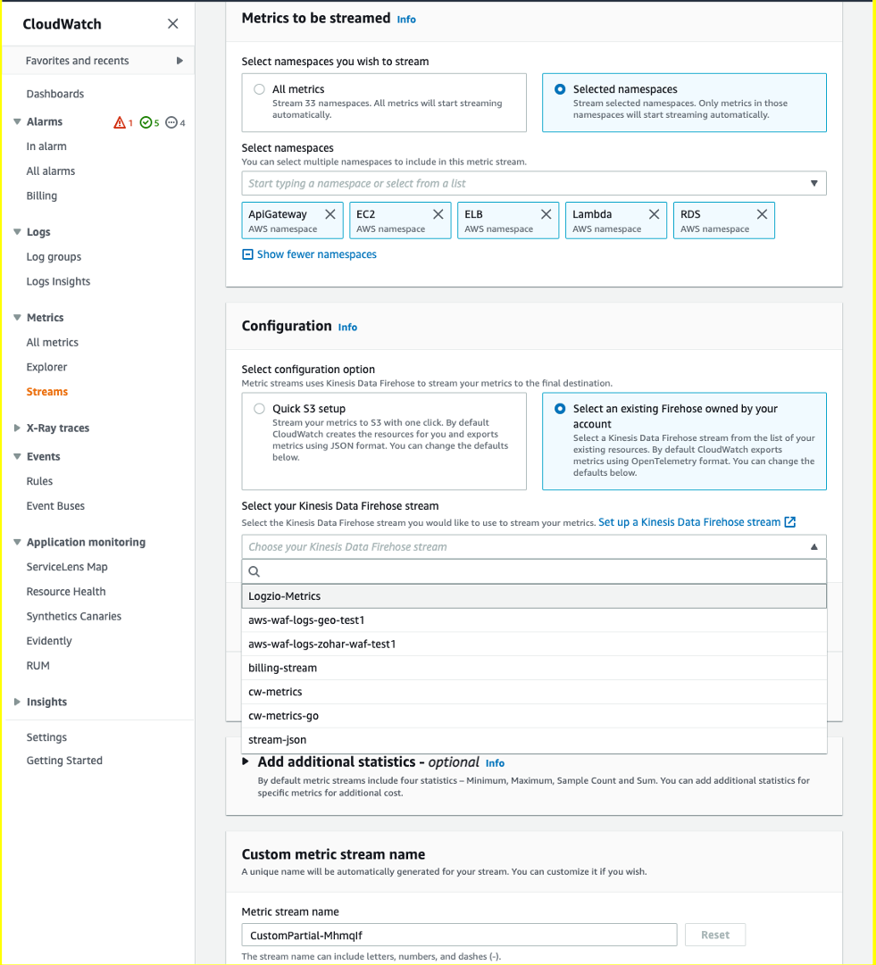
If you’d like, you can choose additional statistics in the Add additional statistics box, which provides helpful metrics in terms of percentiles to monitor like latency metrics (i.e., which services have the highest average latency). This may increase your costs.
- Lastly, give your metric stream a name and hit Create metric stream.
That’s it! Without writing a single line of code, we configured an integration with AWS and Logz.io that enables fast and easy infrastructure monitoring through Amazon CloudWatch data collection.
Your metrics will be stored in Logz.io for 18 months out of the box, without requiring any overhead management.
You can also begin to build dashboards and alerts to begin monitoring – like this Amazon EC2 monitoring dashboard below.
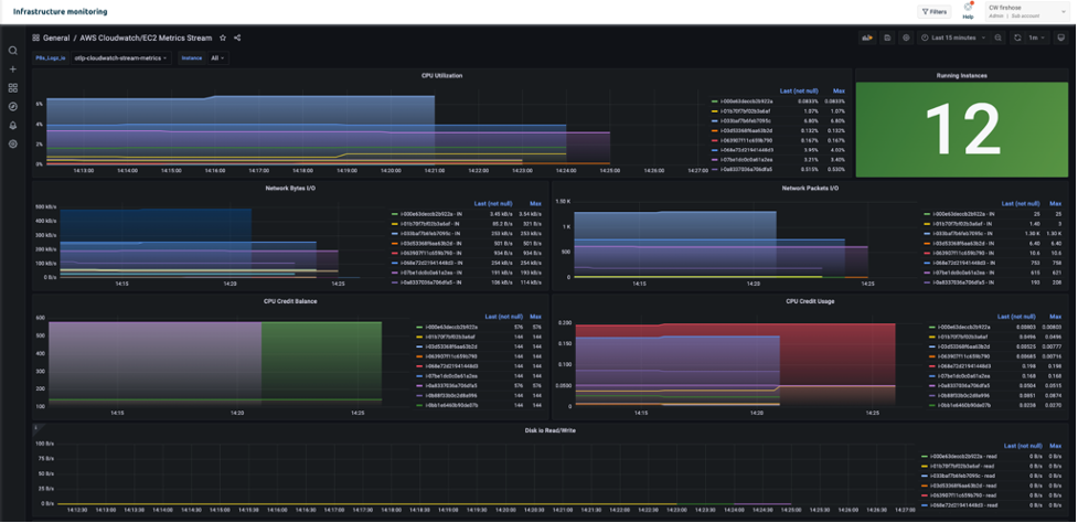
Conclusion
This post demonstrated how to configure an integration with AWS and Logz.io for efficient infrastructure monitoring through Amazon CloudWatch.
To learn more about building metrics dashboards in Logz.io, you can watch this video.
Currently, some users might find that they are sending more data than they really need, which can raise costs. In future versions of this integration, it will be easier to narrow down the metrics to reduce costs.
Want to try it yourself? Create a Logz.io account today, navigate to our infrastructure monitoring product, and start streaming metric data to Logz.io to start monitoring.
About the authors
Amos Etzion – Product Manager at Logz.io
Charlie Klein – Product Marketing Manager at Logz.io
Mark Kriaf – Partner Solutions Architect at AWS
Delta Lake is an open-source project that helps implement modern data lake architectures commonly built on Amazon S3 or other cloud storages. With Delta Lake, you can achieve ACID transactions, time travel queries, CDC, and other common use cases on the cloud. Delta Lake is available with multiple AWS services, such as AWS Glue Spark jobs, Amazon EMR, Amazon Athena, and Amazon Redshift Spectrum.
AWS Glue includes Delta crawler, a capability that makes discovering datasets simpler by scanning Delta Lake transaction logs in Amazon Simple Storage Service (Amazon S3), extracting their schema, creating manifest files in Amazon S3, and automatically populating the AWS Glue Data Catalog, which keeps the metadata current. The newly created AWS Glue Data Catalog table has format SymlinkTextInputFormat. Delta crawler creates a manifest file, which is a text file containing the list of data files that query engines such as Presto, Trino, or Athena can use to query the table rather than finding the files with the directory listing. A previous blog post demonstrated how it works. Manifest files needed to be regenerated on a periodic basis to include newer transactions in the original Delta Lake tables which resulted in expensive I/O operations, longer processing times, and increased storage footprint.
With today’s launch, Glue crawler is adding support for creating AWS Glue Data Catalog tables for native Delta Lake tables and does not require generating manifest files. This improves customer experience because now you don’t have to regenerate manifest files whenever a new partition becomes available or a table’s metadata changes. With the native Delta Lake tables and automatic schema evolution with no additional manual intervention, this reduces the time to insight by making newly ingested data quickly available for analysis with your preferred analytics and machine learning (ML) tools.
Amazon Athena SQL engine version 3 started supporting Delta Lake native connector. AWS Glue for Apache Spark also started supporting Delta Lake native connector in Glue version 3.0 and later. Amazon EMR started supporting Delta Lake in EMR release version 6.9.0 and later. It means that you can query the Delta transaction log directly in Amazon Athena, AWS Glue for Apache Spark, and Amazon EMR. It makes the experience of working with native Delta Lake tables seamless across the platforms.
This post demonstrates how AWS Glue crawlers work with native Delta Lake tables and describes typical use cases to query native Delta Lake tables.
How AWS Glue crawler works with native Delta Lake tables
Now AWS Glue crawler has two different options:
- Native table: Create a native Delta Lake table definition on AWS Glue Data Catalog.
- Symlink table: Create a symlink-based manifest table definition on AWS Glue Data Catalog from a Delta Lake table, and generate its symlink files on Amazon S3.
Native table
Native Delta Lake tables are accessible from Amazon Athena (engine version 3), AWS Glue for Apache Spark (Glue version 3.0 and later), Amazon EMR (release version 6.9.0 and later), and other platforms that support Delta Lake tables. With the native Delta Lake tables, you have the capabilities such as ACID transactions, all while needing to maintain just a single source of truth.
Symlink table
Symlink tables are a consistent snapshot of a native Delta Lake table, represented using the SymlinkTextInputFormat using parquet files. The symlink tables are accessible from Amazon Athena and Amazon Redshift Spectrum.
Since the symlink tables are a snapshot of the original native Delta Lake tables, you need to maintain both the original native Delta Lake tables and the symlink tables. When the data or schema in an original Delta Lake table is updated, the symlink tables in the AWS Glue Data Catalog may become out of sync. It means that you can still query the symlink table and get a consistent result, but the result of the table is at the previous point in time.
Crawl native Delta Lake tables using AWS Glue crawler
In this section, let’s go through how to crawl native Delta Lake tables using AWS Glue crawler.
Prerequisite
Here’s the prerequisite for this tutorial:
- Install and configure AWS Command Line Interface (AWS CLI).
- Create your S3 bucket if you do not have it.
- Create your IAM role for AWS Glue crawler if you do not have it.
- Run the following command to copy the sample Delta Lake table into your S3 bucket. (Replace your\_s3\_bucket with your S3 bucket name.)
Create a Delta Lake crawler
A Delta Lake crawler can be created through the AWS Glue console, AWS Glue SDK, or AWS CLI. Specify a DeltaTarget with the following configurations:
DeltaTables– A list of S3DeltaPathswhere the Delta Lake tables are located. (Note that each path must be the parent of a\_delta\_logfolder. If the Delta transaction log is located ats3://bucket/sample\_delta\_table/\_delta\_log, then the paths3://bucket/sample\_delta\_table/should be provided.WriteManifest– A Boolean value indicating whether or not the crawler should write the manifest files for eachDeltaPath. This parameter is only applicable for Delta Lake tables created via manifest filesCreateNativeDeltaTable– A Boolean value indicating whether the crawler should create a native Delta Lake table. If set toFalse, the crawler would create a symlink table instead. Note that bothWriteManifestandCreateNativeDeltaTableoptions can’t be set toTrue.ConnectionName– An optional connection name stored in the Data Catalog that the crawler should use to access Delta Lake tables backed by a VPC.
In this instruction, create the crawler through the console. Complete the following steps to create a Delta Lake crawler:
- Open the AWS Glue console.
- Choose Crawlers.
- Choose Create crawler.
- For Name, enter delta-lake-native-crawler, and choose Next.
- Under Data sources, choose Add a data source.
- For Data source, select Delta Lake.
- For Include delta lake table path(s), enter
s3://your\_s3\_bucket/data/sample\_delta\_table/. - For Create tables for querying, choose Create Native tables,
- Choose Add a Delta Lake data source.

- Choose Next.
- For Existing IAM role, choose your IAM role, then choose Next.
- For Target database, choose Add database, then Add database dialog appears. For Database name, enter
delta\_lake\_native, then choose Create. Choose Next. - Choose Create crawler.
- The Delta Lake crawler can be triggered to run through the console or through the SDK or AWS CLI using the
StartCrawlAPI. It could also be scheduled through the console to trigger the crawlers at specific times. In this instruction, run the crawler through the console. - Select
delta-lake-native-crawler, and choose Run. - Wait for the crawler to complete.
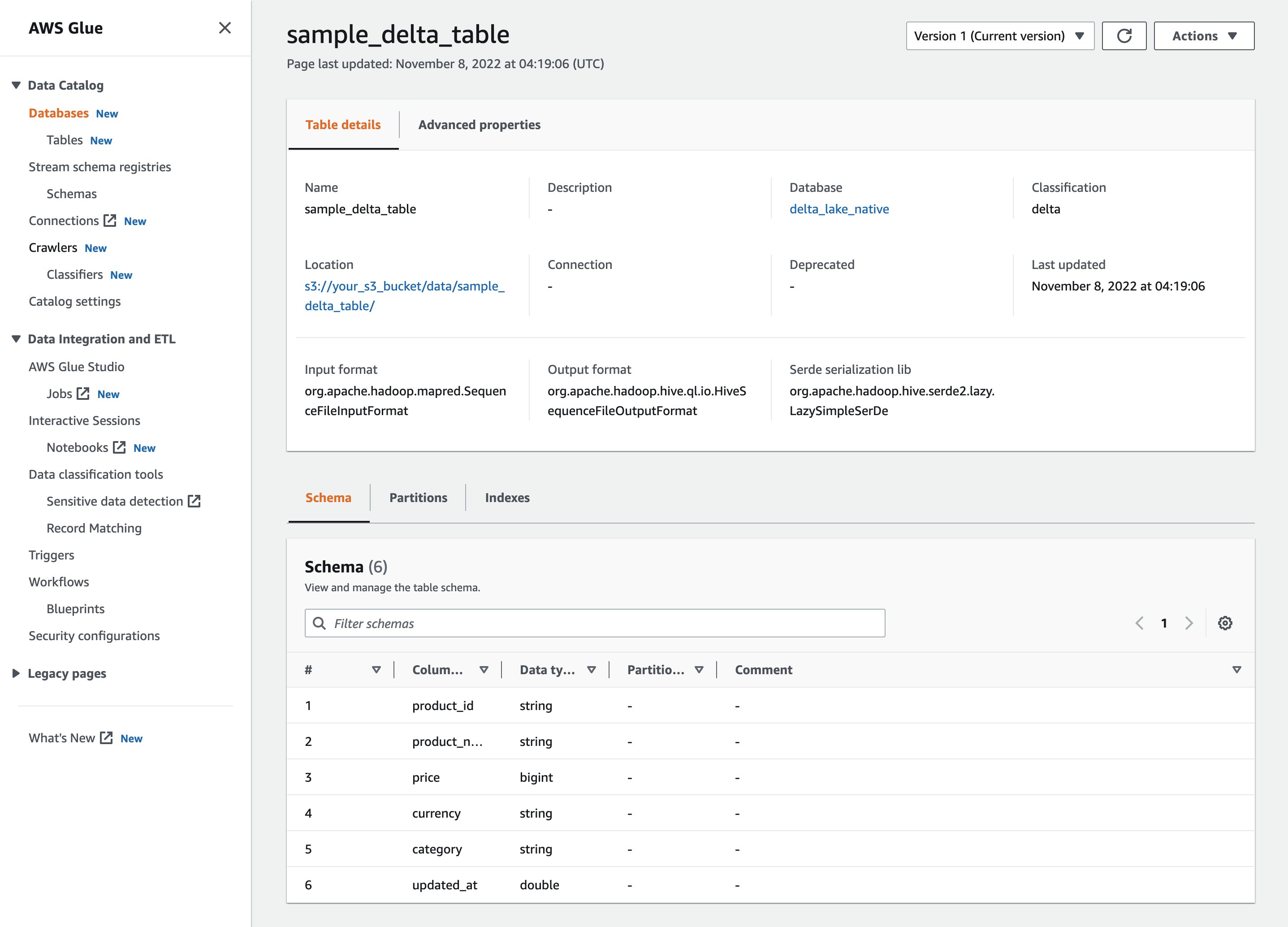
After the crawler has run, you can see the Delta Lake table definition in the AWS Glue console:
You can also verify an AWS Glue table definition through the following AWS CLI command:
After you create the table definition on AWS Glue Data Catalog, AWS analytics services such as Athena and AWS Glue Spark jobs are able to query the Delta Lake table.
Query Delta Lake tables using Amazon Athena
Amazon Athena is an interactive query service that makes it easy to analyze data in Amazon Simple Storage Service (Amazon S3) using standard SQL. Athena is serverless, so there is no infrastructure to manage, and you pay only for the queries that you run on datasets at petabyte scale. You can use Athena to query your S3 data lake for use cases such as data exploration for machine learning (ML) and AI, business intelligence (BI) reporting, and ad hoc querying.
There are now two ways to use Delta Lake tables in Athena:
- For native table: Use Athena’s newly launched native support for Delta Lake tables. You can learn more in Querying Delta Lake tables. This method no longer requires regenerating manifest files after every transaction. Data updates are available for queries in Athena as soon as they are performed in the original Delta Lake tables, and you get up to 40 percent improvement in query performance over querying manifest files. Since Athena optimizes data scans in native Delta Lake queries using statistics in Delta Lake files, you get the advantage of reduced cost for Athena queries. This post focuses on this approach.
- For symlink table: Use
SymlinkTextInputFormatto query symlink tables through manifest files generated from Delta Lake tables. This was previously the only manner in which Delta Lake table querying was supported via Athena and is no longer recommended when you use only Athena to query the Delta Lake tables.
To use the native Delta Lake connector in Athena, you need to use Athena engine version 3. If you are using an older engine version, change the engine version.
Complete following steps to start queries on Athena:
- Open the Amazon Athena console.
- Run the following query.
The following screenshot shows our output:

Query Delta Lake tables using AWS Glue for Apache Spark
AWS Glue for Apache Spark natively supports Delta Lake. AWS Glue version 3.0 (Apache Spark 3.1.1) supports Delta Lake 1.0.0, and AWS Glue version 4.0 (Apache Spark 3.3.0) supports Delta Lake 2.1.0. With this native support for Delta Lake, what you need for configuring Delta Lake is to provide a single job parameter --datalake-formats delta. There is no need to configure a separate connector for Delta Lake in AWS Marketplace. It reduces the configuration steps required to use these frameworks in AWS Glue for Apache Spark.
AWS Glue also provides a serverless notebook interface called AWS Glue Studio notebook to query and process data interactively. Complete the following steps to launch AWS Glue Studio notebook and query a Delta Lake table:
- On the AWS Glue console, choose Jobs in the navigation plane.
- Under Create job, select Jupyter Notebook.

- Choose Create a new notebook from scratch, and choose Create.
- For Job name, enter
delta-sql. - For IAM role, choose your IAM role. If you don’t have your own role for the AWS Glue job, create it by following the steps documented in the AWS Glue Developer Guide.
- Choose Start notebook job.
- Copy and paste the following code to the first cell and run the cell.
- Run the existing cell containing the following code.
- Copy and paste the following code to the third cell and run the cell.
The following screenshot shows our output:

Clean up
Now for the final step, cleaning up the resources:
- Delete your data under your S3 path:
s3://your\_s3\_bucket/data/sample\_delta\_table/. - Delete the AWS Glue crawler
delta-lake-native-crawler. - Delete the AWS Glue database
delta\_lake\_native. - Delete the AWS Glue notebook job
delta-sql.
Conclusion
This post demonstrated how to crawl native Delta Lake tables using an AWS Glue crawler and how to query the crawled tables from Athena and Glue Spark jobs. Start using AWS Glue crawlers for your own native Delta Lake tables.
If you have comments or feedback, please feel free to leave them in the comments.
About the authors
Noritaka Sekiyama is a Principal Big Data Architect on the AWS Glue team. He works based in Tokyo, Japan. He is responsible for building software artifacts to help customers. In his spare time, he enjoys cycling with his road bike.
 Kyle Duong is a Software Development Engineer on the AWS Glue and Lake Formation team. He is passionate about building big data technologies and distributed systems. In his free time, he enjoys cycling or playing basketball.
Sandeep Adwankar is a Senior Technical Product Manager at AWS. Based in the California Bay Area, he works with customers around the globe to translate business and technical requirements into products that enable customers to improve how they manage, secure, and access data.
Today, hundreds of thousands of customers use data lakes for analytics and machine learning. However, data engineers have to cleanse and prepare this data before it can be used. The underlying data has to be accurate and recent for customer to make confident business decisions. Otherwise, data consumers lose trust in the data and make suboptimal or incorrect decisions. It is a common task for data engineers to evaluate whether the data is accurate and recent or not. Today there are various data quality tools. However, common data quality tools usually require manual processes to monitor data quality.
AWS Glue Data Quality is a preview feature of AWS Glue that measures and monitors the data quality of Amazon Simple Storage Service (Amazon S3) data lakes and in AWS Glue extract, transform, and load (ETL) jobs. This is an open preview feature so it is already enabled in your account in the available Regions. You can easily define and measure the data quality checks in AWS Glue Studio console without writing codes. It simplifies your experience of managing data quality.
This post is Part 2 of a four-post series to explain how AWS Glue Data Quality works. Check out the previous post in this series:
Getting started with AWS Glue Data Quality
|
In this post, we show how to create an AWS Glue job that measures and monitors the data quality of a data pipeline. We also show how to take action based on the data quality results.
Solution overview
Let’s consider an example use case in which a data engineer needs to build a data pipeline to ingest the data from a raw zone to a curated zone in a data lake. As a data engineer, one of your key responsibilities—along with extracting, transforming, and loading data—is validating the quality of data. Identifying data quality issues upfront helps you prevent placing bad data in the curated zone and avoid arduous data corruption incidents.
In this post, you’ll learn how to easily set up built-in and custom data validation checks in your AWS Glue job to prevent bad data from corrupting the downstream high-quality data.
The dataset used for this post is synthetically generated; the following screenshot shows an example of the data.

Set up resources with AWS CloudFormation
This post includes an AWS CloudFormation template for a quick setup. You can review and customize it to suit your needs.
The CloudFormation template generates the following resources:
- An Amazon Simple Storage Service (Amazon S3) bucket (
gluedataqualitystudio-*). - The following prefixes and objects in the S3 bucket:
datalake/raw/customer/customer.csvdatalake/curated/customer/scripts/sparkHistoryLogs/temporary/
- AWS Identity and Access Management (IAM) users, roles, and policies. The IAM role (
GlueDataQualityStudio-*) has permission to read and write from the S3 bucket. - AWS Lambda functions and IAM policies required by those functions to create and delete this stack.
To create your resources, complete the following steps:
- Sign in to the AWS CloudFormation console in the
us-east-1Region. - Choose Launch Stack:
- Select I acknowledge that AWS CloudFormation might create IAM resources.
- Choose Create stack and wait for the stack creation step to complete.

Implement the solution
To start configuring your solution, complete the following steps:
- On the AWS Glue Studio console, choose Jobs in the navigation pane.

- Select Visual with a blank canvas and choose Create.

- Choose the Job Details tab to configure the job.

- For Name, enter
GlueDataQualityStudio. - For IAM Role, choose the role starting with
GlueDataQualityStudio-*. - For Glue version, choose Glue 3.0.
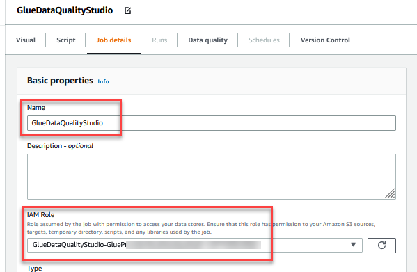
- For Job bookmark, choose Disable. This allows you to run this job multiple times with the same input dataset.
- For Number of retries, enter
0.

- In the Advanced properties section, provide the S3 bucket created by the CloudFormation template (starting with
gluedataqualitystudio-*).
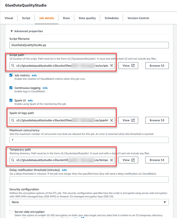
- Choose Save.

- After the job is saved, choose the Visual tab and on the Source menu, choose Amazon S3.
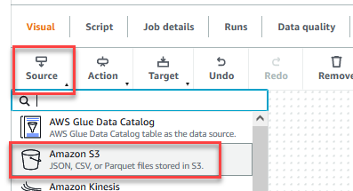
- On the Data source properties – S3 tab, for S3 source type, select S3 location.
- Choose Browse S3 and navigate to prefix
/datalake/raw/customer/in the S3 bucket starting withgluedataqualitystudio-*. - Choose Infer schema.

- On the Action menu, choose Evaluate Data Quality.
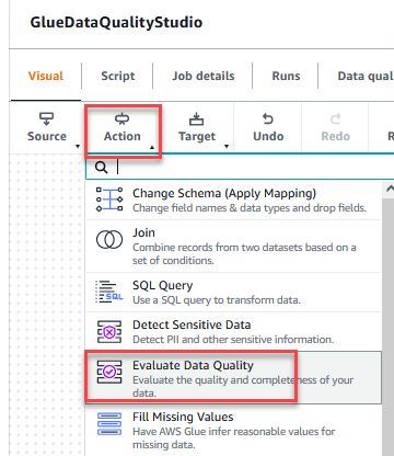
- Choose the Evaluate Data Quality node.

On the Transform tab, you can now start building data quality rules. The first rule you create is to check ifCustomer\_IDis unique and not null using theisPrimaryKeyrule. - On the Rule types tab of the DQDL rule builder, search for
isprimarykeyand choose the plus sign.

- On the Schema tab of the DQDL rule builder, choose the plus sign next to
Customer\_ID. - In the rule editor, delete
id.
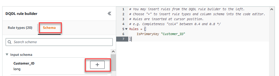
The next rule we add checks that theFirst\_Namecolumn value is present for all the rows. - You can also enter the data quality rules directly in the rule editor. Add a comma (,) and enter
IsComplete "First\_Name",after the first rule.

Next, you add a custom rule to validate that no row exists withoutTelephoneorEmail. - Enter the following custom rule in the rule editor:
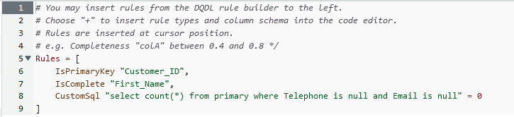
The Evaluate Data Quality feature provides actions to manage the outcome of a job based on the job quality results. - For this post, select Fail job when data quality fails and choose Fail job without loading target data actions. In the Data quality output setting section, choose Browse S3 and navigate to prefix
dqresultsin the S3 bucket starting withgluedataqualitystudio-*.

- On the Target menu, choose Amazon S3.

- Choose the Data target – S3 bucket node.
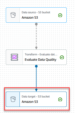
- On the Data target properties – S3 tab, for Format, choose Parquet, and for Compression Type, choose Snappy.
- For S3 Target Location, choose Browse S3 and navigate to the prefix
/datalake/curated/customer/in the S3 bucket starting withgluedataqualitystudio-*.

- Choose Save, then choose Run.
 You can view the job run details on the Runs tab. In our example, the job fails with the error message “AssertionError: The job failed due to failing DQ rules for node: <node>.”
 You can review the data quality result on the Data quality tab. In our example, the custom data quality validation failed because one of the rows in the dataset had no
 TelephoneorEmailvalue. Evaluate Data Quality results is also written to the S3 bucket in JSON format based on the data quality result location parameter of the node.
 - Navigate to
dqresultsprefix under the S3 bucket startinggluedataqualitystudio-*. You will see that the data quality result is partitioned by date.

The following is the output of the JSON file. You can use this file output to build custom data quality visualization dashboards.

You can also monitor the Evaluate Data Quality node through Amazon CloudWatch metrics and set alarms to send notifications about data quality results. To learn more on how to set up CloudWatch alarms, refer to Using Amazon CloudWatch alarms.

Clean up
To avoid incurring future charges and to clean up unused roles and policies, delete the resources you created:
- Delete the
GlueDataQualityStudiojob you created as part of this post. - On the AWS CloudFormation console, delete the
GlueDataQualityStudiostack.
Conclusion
AWS Glue Data Quality offers an easy way to measure and monitor the data quality of your ETL pipeline. In this post, you learned how to take necessary actions based on the data quality results, which helps you maintain high data standards and make confident business decisions.
To learn more about AWS Glue Data Quality, check out the documentation:
- Evaluating data quality with AWS Glue Studio
- AWS Glue Data Quality (preview)
- To dive into the AWS Glue Data Quality APIs, take a look at the documentation: Data Quality API
About the Authors
Deenbandhu Prasad is a Senior Analytics Specialist at AWS, specializing in big data services. He is passionate about helping customers build modern data architecture on the AWS Cloud. He has helped customers of all sizes implement data management, data warehouse, and data lake solutions.
 Yannis Mentekidis is a Senior Software Development Engineer on the AWS Glue team.
AWS Glue is a serverless data integration service that makes it simple to discover, prepare, and combine data for analytics, machine learning (ML), and application development. You can use AWS Glue to create, run, and monitor data integration and ETL (extract, transform, and load) pipelines and catalog your assets across multiple data stores.
Hundreds of thousands of customers use data lakes for analytics and machine learning to make data-driven business decisions. Data consumers lose trust in data if it is not accurate and recent, making data quality essential for undertaking optimal and correct decisions.
Evaluation of the accuracy and freshness of data is a common task for engineers. Currently, there are various tools available to evaluate data quality. However, these tools often require manual processes of data discovery and expertise in data engineering and coding.
We are pleased to announce the public preview launch of AWS Glue Data Quality. You can access this feature today without requesting any additional access in the available Regions. AWS Glue Data Quality is a new preview feature of AWS Glue that measures and monitors the data quality of Amazon S3-based data lakes and in AWS Glue ETL jobs. It does not require any expertise in data engineering or coding. It simplifies your experience of monitoring and evaluating the quality of your data.
This is Part 1 of a four-part series of posts to explain how AWS Glue Data Quality works. Check out the next posts in the series:
Getting started with AWS Glue Data Quality
|
In this post, we will go over the simplicity of using the AWS Glue Data Quality feature by:
- Starting data quality recommendations and runs on your data in AWS Glue Data Catalog.
- Creating an Amazon CloudWatch alarm for getting notifications when data quality results are below a certain threshold.
- Analyzing your AWS Glue Data Quality run results through Amazon Athena.
Set up resources with AWS CloudFormation
The provided CloudFormation script creates the following resources for you:
- The IAM role required to run AWS Glue Data Quality runs
- An Amazon Simple Storage Service (Amazon S3) bucket to store the NYC Taxi dataset
- An S3 bucket to store and analyze the results of AWS Glue Data Quality runs
- An AWS Glue database and table created from the NYC Taxi dataset
- Template: GlueDQBlog.json
- Data used: yellow\_tripdata\_2022-01.parquet
- Malformed data used in Section 2 of this blog: malformed\_yellow\_tripdata.parquet
Steps:
- Open the AWS CloudFormation console.
- Choose Create stack and then select With new resources (standard).

- For Template source, choose Upload a template File, and provide the above attached template file. Then choose Next.

- For Stack name, DataQualityDatabase, and DataQualityTable, leave as default. For DataQualityS3BucketName, enter the name of your S3 bucket. Then choose Next.

- On the final screen, make sure to acknowledge that this stack would create IAM resources for you, and choose Submit.

- Once the stack is successfully created, navigate to the S3 bucket created by the stack and upload the yellow\_tripdata\_2022-01.parquet file.
Start an AWS Glue Data Quality run on your data in AWS Glue Data Catalog
In this first section, we will generate data quality rule recommendations from the AWS Glue Data Quality service. Using these recommendations, we will then run a data quality task against our dataset to obtain an analysis of our data.
To get started, complete the following steps:
- Open AWS Glue console.
- Choose Tables under Data Catalog.
- Select the DataQualityTable table created via the CloudFormation stack.
- Select the Data quality tab.

- Choose Recommend ruleset.

- On the Recommend data quality rules page, check Save recommended rules as a ruleset. This will allow us to save the recommended rules in a ruleset automatically, for use in the next steps.
- For IAM Role, choose the IAM role that was created from the CloudFormation stack.
- For Additional configurations -optional, leave the default number of workers and timeout.
- Choose Recommend ruleset. This will start a data quality recommendation run, with the given number of workers.

- Wait for the ruleset to be completed.
- Once completed, navigate back to the Rulesets tab. You should see a successful recommendation run and a ruleset created.

Understand AWS Glue Data Quality recommendations
AWS Glue Data Quality recommendations are suggestions generated by the AWS Glue Data Quality service and are based on the shape of your data. These recommendations automatically take into account aspects like RowCounts, Mean, Standard Deviation etc. of your data, and generate a set of rules, for you to use as a starting point.
The dataset used here was the NYC Taxi dataset. Based on this, the columns in this dataset, and the values of those columns, AWS Glue Data Quality recommends a set of rules. In total, the recommendation service automatically took into consideration all the columns of the dataset, and recommended 55 rules.
Some of these rules are:
- “RowCount between <> and <> ” → Expect a count of number of rows based on the data it saw
- “ColumnValues “VendorID” in [ ] → Expect the ”VendorID“ column to be within a specific set of values
- IsComplete “VendorID” → Expect the “VendorID” to be a non-null value

How do I use the recommended AWS Glue Data Quality rules?
- From the Rulesets section, you should see your generated ruleset. Select the generated ruleset, and choose Evaluate ruleset.
- If you didn’t check the box to Save recommended rules as a ruleset when you ran the recommendation, you can still click on the recommendation task run and copy the rules to create a new ruleset

- If you didn’t check the box to Save recommended rules as a ruleset when you ran the recommendation, you can still click on the recommendation task run and copy the rules to create a new ruleset
- For Data quality actions under Data quality properties, select Publish metrics to Amazon CloudWatch. If this box isn’t checked, the data quality run will not publish metrics to Amazon CloudWatch.
- For IAM role, select the GlueDataQualityBlogRole created in the AWS CloudFormation stack.
- For Requested number of workers under Advanced properties, leave as default.
- For Data quality results location, select the value of the GlueDataQualityResultsS3Bucket location that was created via the AWS CloudFormation stack
- Choose Evaluate ruleset.

- Once the run begins, you can see the status of the run on the Data quality results tab.
- After the run reaches a successful stage, select the completed data quality task run, and view the data quality results shown in Run results.

Our recommendation service suggested that we enforce 55 rules, based on the column values and the data within our NYC Taxi dataset. We then converted the collection of 55 rules into a RuleSet. Then, we ran a Data Quality Evaluation task run using our RuleSet against our dataset. In our results above, we see the status of each within the RuleSet.
You can also utilize the AWS Glue Data Quality APIs to carry out these steps.
Get Amazon SNS notifications for my failing data quality runs through Amazon CloudWatch alarms
Each AWS Glue Data Quality evaluation run from the Data Catalog, emits a pair of metrics named glue.data.quality.rules.passed (indicating a number of rules that passed) and glue.data.quality.rules.failed (indicating the number of failed rules) per data quality run. This emitted metric can be used to create alarms to alert users if a given data quality run falls below a threshold.
To get started with setting up an alarm that would send an email via an Amazon SNS notification, follow the steps below:
- Open Amazon CloudWatch console.
- Choose All metrics under Metrics. You will see an additional namespace under Custom namespaces titled Glue Data Quality.
Note: When starting an AWS Glue Data Quality run, make sure the Publish metrics to Amazon CloudWatch checkbox is enabled, as shown below. Otherwise, metrics for that particular run will not be published to Amazon CloudWatch.

- Under the Glue Data Quality namespace, you should be able to see metrics being emitted per table, per ruleset. For the purpose of our blog, we shall be using the glue.data.quality.rules.failed rule and alarm, if this value goes over 1 (indicating that, if we see a number of failed rule evaluations greater than 1, we would like to be notified).

- In order to create the alarm, choose All alarms under Alarms.
- Choose Create alarm.
- Choose Select metric.

- Select the glue.data.quality.rules.failed metric corresponding to the table you’ve created, then choose Select metric.

- Under the Specify metric and conditions tab, under the Metrics section:
- For Statistic, select Sum.
- For Period, select 1 minute.
- Under the Conditions section:
- For Threshold type, choose Static.
- For Whenever glue.data.quality.rules.failed is…, select Greater/Equal.
- For than…, enter 1 as the threshold value.
- Expand the Additional configurations dropdown and select Treat missing data as good
These selections imply that if the glue.data.quality.rules.failed metric emits a value greater than or equal to 1, we will trigger an alarm. However, if there is no data, we will treat it as acceptable.
- Choose Next.


- On Configure actions:
- For the Alarm state trigger section, select In alarm .
- For Send a notification to the following SNS topic, choose Create a new topic to send a notification via a new SNS topic.
- For Email endpoints that will receive the notification…, enter your email address. Choose Next.
- For Alarm name, enter myFirstDQAlarm, then choose Next.
- Finally, you should see a summary of all the selections on the Preview and create screen. Choose Create alarm at the bottom.
- You should now be able to see the alarm being created from the Amazon CloudWatch alarms dashboard.
In order to demonstrate AWS Glue Data Quality alarms, we are going to go over a real-world scenario where we have corrupted data being ingested, and how we could use the AWS Glue Data Quality service to get notified of this, using the alarm we created in the previous steps. For this purpose, we will use the provided file malformed\_yellow\_taxi.parquet that contains data that has been tweaked on purpose.
- Navigate to the S3 location DataQualityS3BucketName mentioned in the CloudFormation template supplied at the beginning of the blog post.
- Upload the malformed\_yellow\_tripdata.parquet file to this location. This will help us simulate a flow where we have a file with poor data quality coming into our data lakes via our ETL processes.
- Navigate to the AWS Glue Data Catalog console, select the demo\_nyc\_taxi\_data\_input that was created via the provided AWS CloudFormation template and then navigate to the Data quality tab.
- Select the RuleSet we had created in the first section. Then select Evaluate ruleset.
- From the Evaluate data quality screen:
- Check the box to Publish metrics to Amazon CloudWatch. This checkbox is needed to ensure that the failure metrics are emitted to Amazon CloudWatch.
- Select the IAM role created via the AWS CloudFormation template.
- Optionally, select an S3 location to publish your AWS Glue Data Quality results.
- Select Evaluate ruleset.
- Navigate to the Data Quality results tab. You should now see two runs, one from the previous steps of this blog and one that we currently triggered. Wait for the current run to complete.
- As you see, we have a failed AWS Glue Data Quality run result, with only 52 of our original 55 rules passing. These failures are attributed to the new file we uploaded to S3.
- Navigate to the Amazon CloudWatch console and select the alarm we created at the beginning of this section.
- As you can see, we configured the alarm to fire every time the glue.data.quality.rules.failed metric crosses a threshold of 1. After the above AWS Glue Data Quality run, we see 3 rules failing, which triggered the alarm. Further, you also should have gotten an email detailing the alarm’s firing.
We have thus demonstrated an example where incoming malformed data, coming into our data lakes can be identified via the AWS Glue Data Quality rules, and subsequent alerting mechanisms can be created to notify appropriate personas.
Analyze your AWS Glue Data Quality run results through Amazon Athena
In scenarios where you have multiple AWS Glue Data Quality run results against a dataset, over a period of time, you might want to track the trends of the dataset’s quality over a period of time. To achieve this, we can export our AWS Glue Data Quality run results to S3, and use Amazon Athena to run analytical queries against the exported run. The results can then be further used in Amazon QuickSight to build dashboards to have a graphical representation of your data quality trends
In the third part of this post, we will see the steps needed to start tracking data on your dataset’s quality:
- For our data quality runs that we set up in the previous sections, we set the Data quality results location parameter to the bucket location specified by the AWS CloudFormation stack.
- After each successful run, you should see a single JSONL file being exported to your selected S3 location, corresponding to that particular run.
- Open the Amazon Athena console.
- In the query editor, run the following CREATE TABLE statement (replace the <my\_table\_name> with a relevant value, and <GlueDataQualityResultsS3Bucket\_from\_cfn> section with the
GlueDataQualityResultsS3Bucketvalue from the provided AWS CloudFormation template): - Once the above table is created, you should be able to run queries to analyze your data quality results.
For example, consider the following query that shows me the failed AWS Glue Data Quality runs against my table demo\_nyc\_taxi\_data\_input within a time window:
The output of the above query shows me details about all the runs with “outcome” = ‘Failed’ that ran against my NYC Taxi dataset table ( “tablename” = ‘demo\_nyc\_taxi\_data\_input’ ). The output also gives me information about the failure reason ( failurereason ) and the values it was evaluated against ( evaluatedmetrics ).
As you can see, we are able to get detailed information about our AWS Glue Data Quality runs, via the run results uploaded to S3, perform more detailed analysis and build dashboards on top of the data.
Clean up
- Navigate to the Amazon Athena console and delete the table created for data quality analysis.
- Navigate to the Amazon CloudWatch console and delete the alarms created.
- If you deployed the sample CloudFormation stack, delete the CloudFormation stack via the AWS CloudFormation console. You will need to empty the S3 bucket before you delete the bucket.
- If you have enabled your AWS Glue Data Quality runs to output to S3, empty those buckets as well.
Conclusion
In this post, we talked about the ease and speed of incorporating data quality rules using the AWS Glue Data Quality feature, into your AWS Glue Data Catalog tables. We also talked about how to run recommendations and evaluate data quality against your tables. We then discussed analyzing the data quality results via Amazon Athena, and the process for setting up alarms via Amazon CloudWatch in order to notify users of failed data quality.
To dive into the AWS Glue Data Quality APIs, take a look at the AWS Glue Data Quality API documentation
To learn more about AWS Glue Data Quality, check out the AWS Glue Data Quality Developer Guide
About the authors
Aniket Jiddigoudar is a Big Data Architect on the AWS Glue team.
 Joseph Barlan is a Frontend Engineer at AWS Glue. He has over 5 years of experience helping teams build reusable UI components and is passionate about frontend design systems. In his spare time, he enjoys pencil drawing and binge watching tv shows.
AWS Marketplace enables independent software vendors (ISVs), data providers, and consulting partners to sell software, services, and data to millions of AWS customers. Working in partnership with the AWS Partner Network (APN), AWS Marketplace helps ISVs and partners build, market and sell their AWS offerings by providing crucial business, technical, and marketing support.
The AWS Marketplace Seller Insights team helps AWS sellers scale their businesses by providing reports, data feeds, and insights. We share this data directly with sellers through the AWS Marketplace Management Portal (AMMP). In 2013, we launched the first version of reporting insights, delivered monthly via static CSV files. To improve the customer experience, the next iteration of reporting upgrades was launched in 2020 and provided more granular data, refreshed daily and delivered via feeds.
We’ve spent the past few months working closely with the QuickSight team and are excited to now offer AWS Marketplace sellers public preview access to two new Amazon QuickSight dashboards. QuickSight improves the reporting experience for AWS Marketplace sellers by making it easy for users to monitor key metrics, perform ad hoc analysis, and quickly get business insights from data at any time and on any device.
In this post, we discuss our decision to implement QuickSight Embedded, as well as some of the benefits to AWS Marketplace sellers.
Data agility is a key differentiator
Making informed decisions is a business-critical function for successful organizations. Being able to quickly view performance trends and adjust strategies accordingly can make all the difference between hitting or missing business goals. Investing time, effort, and resources in technical data integrations, or creating pivot tables and charts from downloaded raw data, means a slower response rate to analyze shifts in performance trends. The more agile we can be in providing fast, efficient access to key performance indicators, the better positioned AWS Marketplace sellers can be to take action based on what their data tells them.
After reviewing customer feedback on their reporting experience, several trends emerged in what would be most helpful to them. First, sellers wanted a visual representation of their data. Second, though some wanted data feeds available to integrate AWS Marketplace data into their own business intelligence tools, others wanted to be able to access and review data without needing to invest technical business intelligence bandwidth in integrating feeds to create more user-friendly reports. Finally, they wanted the ability to easily filter the data, as well as the option to download it. In researching options to provide the reporting experience AWS Marketplace sellers wanted, we found that QuickSight was a perfect fit.
Doing more with data
Billed Revenue and the Collections & Disbursements are two new QuickSight dashboards embedded directly into the AWS Marketplace Management Portal (AMMP), accessed via the Insights tab. These dashboards—pre-built with 10+ controls or filters, 15+ visualizations, and powered by daily refreshed data—provide a visual reporting experience for revenue recognition and disbursements tracking.
The following screenshot shows what the dashboards look like in the Finance operations section on the Insights tab within the AMMP.

The dashboards are divided into several sections:
- Controls provides filters to refine your dashboard data.
- Date Range Filter provides the ability to filter dashboard data based on the dates.
- Metrics, Trends, and Breakdowns all provide detailed analytics to understand business performance.
- Granular data provides the option to download the raw data from the dashboard by clicking on the table and choosing the Export to CSV option.
For quick help, sellers can select the Info button to view the side navigation panel with tips on how to use the dashboard. They can also reach out to our team by selecting Contact us from the Info panel.


Improving the customer experience
The Billed Revenue dashboard now reflects changes within 24 hours of a customer being billed or refunded—a major improvement over the 45 days it once took to access this data from the legacy AMMP Billed Revenue report. Similarly, the Collections & Disbursements dashboard provides disbursement information within 24 hours of AWS sending funds to sellers, whereas it used to take up to 4 days from the legacy AMMP Disbursement Report.
Our team’s decision to go with QuickSight was the direct result of a clear alignment between what our sellers told us they wanted and what QuickSight offered. With QuickSight Embedded dashboards, AWS Marketplace sellers now have a visual representation of their data that doesn’t require time or resources dedicated to technical integration implementations, and they can quickly and easily manipulate the data via filters, or they can download it to a CSV if that’s their preference. Embedded dashboards simplify the viewing, analyzing, and tracking of key business metrics and trends related to financial operations. Being able to easily show each seller only their relevant data (using row-level security) provides us with the flexibility we need, with the peace of mind of knowing everything is secure. AWS Marketplace data is hosted in an Amazon Redshift cluster; QuickSight’s seamless integration into Amazon Redshift made it a fantastic choice.
Data-driven decisions with QuickSight
Embedding these new QuickSight dashboards into the AMMP has enabled us to provide at-a-glance metrics to AWS Marketplace sellers in a faster, more efficient, and far more user-friendly way than ever before. QuickSight has made a significant impact on how quickly sellers can access their data, which helps them respond faster to shifting trends.
To learn more about how you can embed customized data visuals, interactive dashboards, and natural language querying into any application, visit Amazon QuickSight Embedded.
About the Authors
 Snigdha Sahi is a Senior Product Manager (Technical) with Amazon Web Services (AWS) Marketplace. She has diverse work experience across product management, product development and management consulting. A technology enthusiast, she loves brainstorming and building products that are intuitive and easy to use. In her spare time, she enjoys hiking, solving Sudoku and listening to music.
 Vincent Larchet is a Principal Software Development Engineer on the AWS Marketplace team based in Vancouver, BC. Outside of work, he is a passionate wood worker and DIYer.
Amazon EMR Serverless is a serverless option in Amazon EMR that makes it easy for data analysts and engineers to run applications using open-source big data analytics frameworks such as Apache Spark and Hive without configuring, managing, and scaling clusters or servers. You get all the features of the latest open-source frameworks with the performance-optimized runtime of Amazon EMR, and without having to plan and operate instances and clusters.
With Amazon EMR, you can run your analytics applications on dedicated EMR clusters, on existing Amazon Elastic Kubernetes Service (Amazon EKS) clusters, or using the new EMR Serverless deployment option where you don’t have to manage clusters or instances. When you build a Spark or Hive application using an Amazon EMR release, say Amazon EMR 6.8, you can run the application on EMR clusters, on EKS clusters using Amazon EMR on EKS, or using EMR Serverless without having to change the application.
To learn about the benefits of each deployment option in EMR Serverless, refer to What are some of the feature differences between EMR Serverless and Amazon EMR on EC2? in the Amazon EMR FAQ. You can also learn about the pricing for these options from the Amazon EMR pricing page. Many customers already run data analytics applications on EMR clusters, and find that the new serverless option is simpler and less expensive.
In this post, we discuss how you can estimate what it may cost to run an application that currently runs on EMR clusters using the new serverless option, and perform this analysis simply by using your current application metrics. This approach helps you evaluate and adopt the deployment option that is most cost effective for the application. However, the Amazon EMR pricing page doesn’t tell you how you can easily estimate the cost of running your existing EMR cluster applications on EMR Serverless. In the following sections, we describe an approach that enables you to do that.
Although the example in this post discusses how you can get a cost estimate for applications running on EMR clusters, you can also use the approach if you’re running a Spark or Hive application elsewhere, and want to estimate the cost of running it on EMR Serverless. For example, if you run self-managed Spark or Hive applications on Amazon Elastic Compute Cloud (Amazon EC2) clusters, or if you run Spark jobs on AWS Glue, we show you how you can use this approach to estimate the cost of running the application on EMR Serverless.
Estimating the cost of running applications on your EMR cluster
When you run applications on Amazon EMR clusters, you’re separately charged for the following:
- The Amazon EC2 price of running cluster instances (the price for the underlying servers)
- The price for Amazon Elastic Block Store (Amazon EBS) volumes, if you choose to attach EBS volumes
- The Amazon EMR price for the cluster instances
The total cost of running the cluster includes all three. There are a variety of Amazon EC2 pricing options you can choose from, including On Demand, 1-year and 3-year Reserved Instances, Capacity Savings Plans, and Spot Instances. The Amazon EC2 pricing option that you choose determines (a), the Amazon EC2 price. The cost of running the application on EMR clusters is the sum of (a), (b), and (c). You can compute this cost for the lifetime of running the cluster (from the time a cluster is started to the time the cluster is terminated), or for a specific period of time while the cluster is running. We recommend running the former, that is to compute (a), (b), and (c) from the time the cluster is started to the time the cluster is terminated. If you have set up tags for your Amazon EMR cluster, you can easily get the detailed cost report for your EMR cluster using AWS Cost Explorer.
Estimating the cost of running the same applications using EMR Serverless
When you run the same applications using EMR Serverless, you pay for the amount of vCPU, memory, and storage resources consumed by your applications. There is no separate charge for EC2 instances or EBS volumes. And, you only pay for the resources that are actually used by the application and not for EC2 instances provisioned. For example, when running applications on EMR clusters, when an EC2 instance in the cluster is partially utilized (say, 16 GB memory is used out of 64 GB available on the instance, or 4 VCPUs are utilized out of 16 VCPUs available on the instance), or when the EC2 instance is idle (for example, when the instance is initializing or waiting for an application to start), you still incur Amazon EC2, Amazon EMR, and Amazon EBS charges for the full EC2 instance and for the duration that the instance is active in the EMR cluster. With EMR Serverless, you only pay for the vCPU, memory, and storage resources used from the time workers start to run your Spark or Hive job until the time they stop.
To estimate the cost of running your EMR Spark or Hive application on EMR Serverless, you need to first aggregate the total compute vCore-seconds, memory MB-seconds, and storage GB-seconds consumed by each YARN application that ran on your EMR cluster, from the time the YARN container is started to the time the YARN container is terminated. You can obtain these metrics from YARN resource manager logs accessible from YARN timeline server or YARN CLI tools. You can retrieve the running time, vCore-seconds, and memory MB-seconds used by each of the YARN applications.
If your cluster only runs Spark applications, there is a simpler approach to estimate. Instead of obtaining the vCore-seconds, memory MB-seconds, and storage GB-seconds from YARN resource manager logs, you can obtain these metrics from Spark event logs. We have provided the tool EMR Servless Estimator, which can parse the Spark event logs for your applications and provide the aggregated metrics for your cost estimate.
After you get the usage metrics for your application, you can compute the estimated EMR Serverless cost using EMR Serverless pricing. Simply multiple your aggregated vCore-seconds with EMR Serverless vCPU pricing per second, multiply aggregated memory MB-seconds with the EMR Serverless memory pricing per second, and multiply storage GB-seconds with the EMR Serverless storage pricing per second (only if the storage requirements exceed 20 GB per worker). By adding up these costs for vCPU, memory, and storage, you can compare the cost of running the same applications on EMR Serverless.
In this approach, we assume that the performance of the application is equivalent. In other words, the size (vCPU, memory) and runtime duration for each YARN container on the EMR cluster is the same as the number, size, and runtime duration of workers needed to run the application on EMR Serverless. We make this assumption because the EMR runtime for an EMR release is the same regardless of whether the application is run on an EMR cluster or on EMR Serverless.
Example
Let’s do a sample cost comparison of Amazon EMR on EC2 and EMR Serverless using a single cluster.
We ran a Spark application on an EMR cluster with five nodes (one primary, two core, and two task and gathered YARN metrics using the YARN CLI. The following code shows our aggregate resource allocation.

We computed the Amazon EMR on EC2 costs as follows:
- Cluster instances
- Primary: m5.2xlarge:1
- Core: r5.2xlarge:2
- Task: r5.2xlarge:2
- Cluster runtime = 18 min
- Instance on-demand cost
- m5.2xlarge (8 vCPU, 32 GiB memory)
- Amazon EC2: $0.384/hr
- Amazon EMR incremental: $0.096/hr
- r5.2xlarge (8 vCPU, 64 GiB memory)
- Amazon EC2: $0.504/hr
- Amazon EMR incremental: $0.126/hr
- m5.2xlarge (8 vCPU, 32 GiB memory)
The following is the EMR on EC2 cost calculation:
- Amazon EMR cost = ((1 primary node x $0.096/hr) + (2 core nodes x $ 0.126/hr) + (2 task nodes x $0.126/hr)) = $0.60
- Amazon EC2 cost = ((1 primary x $0.384 /hr ) + (2 core nodes x $0.504/hr) + (2 task nodes x $0.504/hr)) = $2.40
- Amazon EMR on EC2 cluster cost/hr = $0.6 + $2.40 = $3/hr * 8/60 hr (runtime in hrs)
The total Amazon EMR on Amazon EC2 cost is $0.40/hr.
To calculate EMR Serverless cost, aggregate the vCore-seconds and memory MB-seconds for the same application you ran previously on the EMR cluster. Then multiply those numbers with the EMR Serverless vCPU and memory price. Our calculation results are as follows:
- Total\_vcore\_seconds = 5737
- Total\_Memory\_mb\_seconds = 120156631
- Convert to vCPU/hr and memory-GB/hr:
- Aggregated vCPU/hr: 5737/(60*60)=1.59
- Aggregated memory/hr: 120156631/(60*60*1024)=32.5
- Total vCPU-hours cost = 33 vCPU * 0.052624 VCPU/hr * 8/60 = $0.23
- Total memory GB cost = 1.59 MB * 0.0057785 memory/hr * 8/60 = $0.00122
In this example, the total EMR Serverless cost is $0.231, a 42% reduction.
Conclusion
Amazon EMR Serverless is a recently launched serverless option in Amazon EMR that makes it easy to run open-source frameworks such as Spark and Hive without configuring, managing, and scaling clusters. Customers that already use EMR clusters want to understand how they can estimate the cost of running their EMR applications using EMR Serverless. We have presented an approach that you can use to conduct a cost analysis based on analyzing application metrics from your EMR clusters.
We hope you give this a try, and share your feedback with us!
About the authors
 Radhika Ravirala is the Principal Product Manager at AWS.
Matthew Liem is the Senior Solution Architecture Manager at AWS.
Recent advances in ease of use and scalability have made streaming data easier to generate and use for real-time decision-making. Coupled with market forces that have forced businesses to react more quickly to industry changes, more and more organizations today are turning to streaming data to fuel innovation and agility.
Amazon Managed Streaming for Apache Kafka (MSK) is a fully managed service that makes it easy to build and run applications that use Apache Kafka, an open-source distributed event streaming platform designed for high-performance data pipelines, streaming analytics, data integration, and mission-critical applications. With Amazon MSK, you can capture real-time data from a wide range of sources such as database change events or web application user clickstreams. Since Kafka is highly optimized for writing and reading fresh data, it’s a great fit for operational reporting. However, gaining insight from this data often requires a specialized stream processing layer to write streaming records to a storage medium like Amazon S3, where it can be accessed by analysts, data scientists, and data engineers for historical analysis and visualization using tools like Amazon QuickSight.
When you want to analyze data where it lives and without developing separate pipelines and jobs, a popular choice is Amazon Athena. With Athena, you can use your existing SQL knowledge to extract insights from a wide range of data sources without learning a new language, developing scripts to extract (and duplicate) data, or managing infrastructure. Athena supports over 25 connectors to popular data sources including Amazon DynamoDB and Amazon Redshift which give data analysts, data engineers, and data scientists the flexibility to run SQL queries on data stored in databases running on-premises or in the cloud alongside data stored in Amazon S3. With Athena, there’s no data movement and you pay only for the queries you run.
What’s new
Starting today, you can now use Athena to query streaming data in MSK and self-managed Apache Kafka. This enables you to run analytical queries on real-time data held in Kafka topics and join that data with other Kafka topics as well as other data in your Amazon S3 data lake – all without the need for separate processes to first store the data on Amazon S3.
Solution overview
In this post, we show you how to get started with real-time SQL analytics using Athena and its connector for MSK. The process involves:
- Registering the schema of your streaming data with AWS Glue Schema Registry. Schema Registry is a feature of AWS Glue that allows you to validate and reliably evolve streaming data against JSON schemas. It can also serialize data into a compressed format, which helps you save on data transfer and storage costs.
- Creating a new instance of the Amazon Athena MSK Connector. Athena connectors are pre-built applications that run as serverless AWS Lambda applications, so there’s no need for standalone data export processes.
- Using the Athena console to run interactive SQL queries on your Kafka topics.
Get started with Athena’s connector for Amazon MSK
In this section, we’ll cover the steps necessary to set up your MSK cluster to work with Athena to run SQL queries on your Kafka topics.
Prerequisites
This post assumes you have a serverless or provisioned MSK cluster set up to receive streaming messages from a producing application. For information, see Setting up Amazon MSK and Getting started using Amazon MSK in the Amazon Managed Streaming for Apache Kafka Developer Guide.
You’ll also need to set up a VPC and a security group before you use the Athena connector for MSK. For more information, see Creating a VPC for a data source connector. Note that with MSK Serverless, VPCs and security groups are created automatically, so you can get started quickly.
Define the schema of your Kafka topics with AWS Glue Schema Registry
To run SQL queries on your Kafka topics, you’ll first need to define the schema of your topics as Athena uses this metadata for query planning. AWS Glue makes it easy to do this with its Schema Registry feature for streaming data sources.
Schema Registry allows you to centrally discover, control, and evolve streaming data schemas for use in analytics applications such as Athena. With AWS Glue Schema Registry, you can manage and enforce schemas on your data streaming applications using convenient integrations with Apache Kafka. To learn more, see AWS Glue Schema Registry and Getting started with Schema Registry.
If configured to do so, the producer of data can auto-register its schema and changes to it with AWS Glue. This is especially useful in use cases where the contents of the data is likely to change over time. However, you can also specify the schema manually and will resemble the following JSON structure.
When setting up your Schema Registry, be sure to give it an easy-to-remember name, such as customer\_schema, because you’ll reference it within SQL queries as you’ll see later on. For additional information on schema set up, see Schema examples for the AWS Glue Schema Registry.
Configure the Athena connector for MSK
With your schema registered with Glue, the next step is to set up the Athena connector for MSK. We recommend using the Athena console for this step. For more background on the steps involved, see Deploying a connector and connecting to a data source.
In Athena, federated data source connectors are applications that run on AWS Lambda and handle communication between your target data source and Athena. When a query runs on a federated source, Athena calls the Lambda function and tasks it with running the parts of your query that are specific to that source. To learn more about the query execution workflow, see Using Amazon Athena Federated Query in the Amazon Athena User Guide.
Start by accessing the Athena console and selecting Data sources on the left navigation, then choose Create data source:

Next, search for and select Amazon MSK from the available connectors and select Next.

In Data source details, give your connector a name, like msk, that’s easy to remember and reference in your future SQL queries. Under Connection details section, select Create Lambda function. This will bring you to the AWS Lambda console where you’ll provide additional configuration properties.
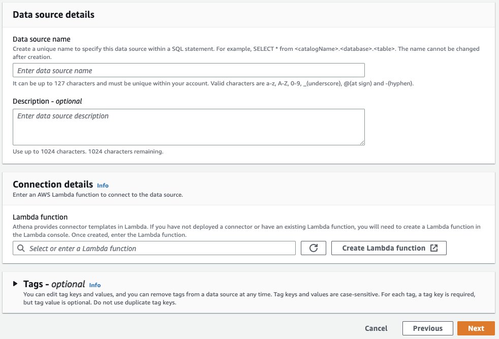
In the Lambda application configuration screen (not shown), you’ll provide the Application settings for your connector. To do this, you’ll need a few properties from your MSK cluster and schema registered in Glue.
On another browser tab, use the MSK console to navigate to your MSK cluster and then select the Properties tab. Here you’ll see the VPC subnets and security group IDs from your MSK cluster which you’ll provide in the SubnetIds and SecurityGroupIds fields in the Athena connector’s Application settings form. You can find the value for KafkaEndpoint by clicking View client information.
In the AWS Glue console, navigate to your Schema Registry to find the GlueRegistryArn for the schema you wish to use with this connector.
After providing these and the other required values, click Deploy.
Return to the Athena console and enter the name of the Lambda function you just created in the Connection details box, then click Create data source.
Run queries on streaming data using Athena
With your MSK data connector set up, you can now run SQL queries on the data. Let’s explore a few use cases in more detail.
Use case: interactive analysis
If you want to run queries that aggregate, group, or filter your MSK data, you can run interactive queries using Athena. These queries will run against the current state of your Kafka topics at the time the query was submitted.
Before running any queries, it may be helpful to validate the schema and data types available within your Kafka topics. To do this, run the DESCRIBE command on your Kafka topic, which appears in Athena as a table, as shown below. In this query, the orders table corresponds to the topic you specified in the Schema Registry.
Now that you know the contents of your topic, you can begin to develop analytical queries. A sample query for a hypothetical Kafka topic containing e-commerce order data is shown below:
Because the orders table (and underlying Kafka topic) can contain an unbounded stream of data, the query above is likely to return a different value for SUM(order\_total) with each execution of the query.
If you have data in one topic that you need to join with another topic, you can do that too:
Use case: ingesting streaming data to a table on Amazon S3
Federated queries run against the underlying data source which ensures interactive queries, like the ones above, are evaluated against the current state of your data. One consideration is that repeatedly running federated queries can put additional load on the underlying source. If you plan to perform multiple queries on the same source data, you can use Athena’s CREATE TABLE AS SELECT, also known as CTAS, to store the results of a SELECT query in a table on Amazon S3. You can then run queries on your newly created table without going back to the underlying source each time.
If you plan to do additional downstream analysis on this data, for example within dashboards on Amazon QuickSight, you can enhance the solution above by periodically adding new data to your table. To learn more, see Using CTAS and INSERT INTO for ETL and data analysis. Another benefit of this approach is that you can secure these tables with row-, column-, and table-level data governance policies powered by AWS Lake Formation to ensure only authorized users can access your table.
What else can you do?
With Athena, you can use your existing SQL knowledge to run federated queries that generate insights from a wide range of data sources without learning a new language, developing scripts to extract (and duplicate) data, or managing infrastructure. Athena provides additional integrations with other AWS services and popular analytics tools and SQL IDEs that allow you to do much more with your data. For example, you can:
- Visualize the data in business intelligence applications like Amazon QuickSight
- Design event-driven data processing workflows with Athena’s integration with AWS Step Functions
- Unify multiple data sources to produce rich input features for machine learning in Amazon SageMaker
Conclusion
In this post, we learned about the newly released Athena connector for Amazon MSK. With it, you can run interactive queries on data held in Kafka topics running in MSK or self-managed Apache Kafka. This helps you bring real-time insights to dashboards or enable point-in-time analysis of streaming data to answer time-sensitive business questions. We also covered how to periodically ingest new streaming data into Amazon S3 without the need for a separate sink process. This simplifies recurring analysis of your data without incurring round-trip queries to your underlying Kafka clusters and makes it possible to secure the data with access rules powered by Lake Formation.
We encourage you to evaluate Athena and federated queries on your next analytics project. For help getting started, we recommend the following resources:
- If you’re new to Athena and want to learn more about its features and capabilities, see Amazon Athena features.
- To learn more about Athena’s connector for MSK, see Amazon Athena MSK Connector.
- For a complete list of supported data sources, see Athena Data Source Connectors.
About the authors
 Scott Rigney is a Senior Technical Product Manager with Amazon Web Services (AWS) and works with the Amazon Athena team based out of Arlington, Virginia. He is passionate about building analytics products that enable enterprises to make data-driven decisions.
Kiran Matty is a Principal Product Manager with Amazon Web Services (AWS) and works with the Amazon Managed Streaming for Apache Kafka (Amazon MSK) team based out of Palo Alto, California. He is passionate about building performant streaming and analytical services that help enterprises realize their critical use cases.
This post was co-written with Mike Zorn, Software Architect at LaunchDarkly as the lead author.
LaunchDarkly’s feature management platform enables customers to release features and measure their impact. As part of this platform, SDKs gather event data, and the event ingestion platform consumes and analyzes this data to measure impact. As the platform launched and customer adoption increased, we had to scale the event data pipeline to meet the demands of the business for new use cases that required zero data loss. We will explain the challenges that we ran into with the initial architecture and the advantages achieved by using Amazon Kinesis Data Streams and additional AWS services in the new architecture. We will also go into the different factors that we considered in the Amazon Kinesis Data Streams implementation for cost efficiency and performance.
Problem statement
LaunchDarkly’s mission is to fundamentally change how companies deliver software by helping them innovate faster, deploy fearlessly, and make each release a masterpiece. With LaunchDarkly, we allow customers to deploy when they want, release when they are ready, and get total control of the code to ship fast, reduce risk, and reclaim their nights and weekends.
In 2017, the event ingestion platform consisted of a fleet of web servers that would write events to several databases, as shown below, that stored event data to power several features of the LaunchDarkly product. These features allow LaunchDarkly’s customers to gain full visibility into how a feature is performing over time, optimize features through experimentation, and quickly verify their implementation. Unfortunately, all of the database writes to power these features were performed within a single process on these web servers, so if any one of these databases had an availability issue, events would queue up in memory until that process ran out of memory and crashed. Since that same database would be used to write data from each web server, all of them would eventually run out of memory and crash. This cycle would repeat itself until the database availability issue was rectified. During that time, there was a permanent loss of all of the event data that was sent by the SDKs.
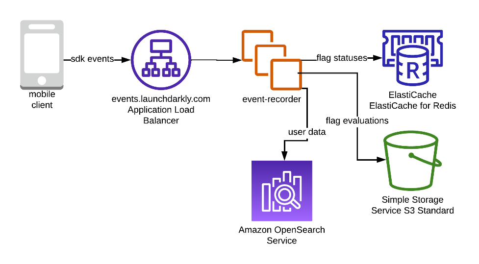
The current system was tolerant of some data loss as the applications that used this data was limited. But the new features and workflows had stringer requirements on data-loss prevention.
We decided to explore alternatives where all the consumers are built with isolated fault tolerance, so each consumer is independent of one another in case of any issues. We built an event-driven pipeline that would be highly durable, scalable, and also provide the ability for data replay. As a result, we scaled from ingesting about 1 TB of data a day to more than 100 TBs of data now.
Solution
The following diagram illustrates our updated design. To support the new use cases, we added Amazon Kinesis Data Streams, AWS Lambda, and Amazon Kinesis Data Firehose to the architecture.
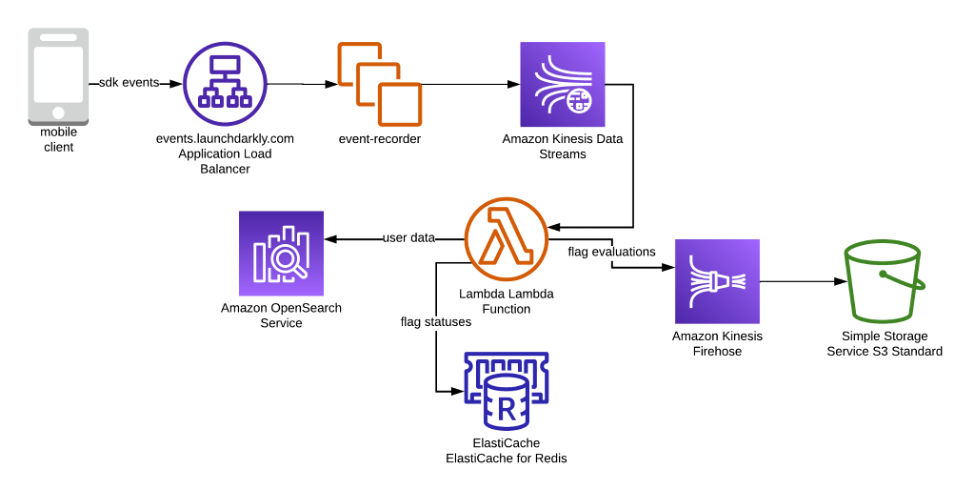
The design has the following key components
- Mobile client using the LaunchDarkly SDK to evaluate feature flags
- Application Load Balancer distributes traffic to Amazon EC2 nodes
- Amazon EC2 nodes run a go application that writes traffic to Amazon Kinesis Data Streams
- Amazon Kinesis Data Streams durably persist data
- AWS Lambda writes various types of data to databases
- Amazon OpenSearch Service records data about users
- Amazon ElastiCache records data about flag statuses
- Amazon Kinesis Firehose batches flag evaluation data and writes it to Amazon S3
- Amazon S3 records data about flag evaluations
Data flows from a LaunchDarkly SDK into the events API, which is backed by an Application Load Balancer (ALB). That ALB routes traffic to a fleet of Amazon EC2 servers. Those servers persist the data to Amazon Kinesis Data Streams. Data is then read out of Amazon Kinesis Data Streams by Lambda functions that transform and write the data in different formats to several databases. The design has a few properties that were very important to this use case.
- Durability
- Isolation
- Data replay
Durability would prevent data loss when issues in data processing arose. Isolation would prevent other consumers of data from failing when one consumer had a failure. Data replay would allow us to debug data anomalies and fix them retroactively.
Amazon Kinesis Data Streams satisfies these three properties. Data written to Amazon Kinesis Data Streams is persisted durably until the data ages out of the stream. Amazon Kinesis Data Streams allows for consumer isolation: each consumer maintains its own iterator position, so consumers can process data from a stream independently of one another. Finally, Amazon Kinesis Data Streams make data replay possible because consumers can set their shard iterator position to be in the past. For example, a consumer can be configured to start reading at 1 hour in the past if the last hour of data needs to be replayed.
A few additional technologies were considered that would allow us to achieve these design properties. Amazon Simple Notification Service (Amazon SNS) combined with Amazon Simple Queue Service (Amazon SQS) would allow for a system with durability and isolation. Data replay was not available out of the box and needed custom implementation to support this feature.
Apache Kafka was also considered, but in spite of the fact that it satisfies these design properties, it was not adopted because the team did not have prior experience with Apache Kafka. Amazon Kinesis Data Streams satisfies these design properties, and it is fully managed, which reduces the need to worry about a lack of operational expertise.
Amazon Kinesis Data Streams implementation deep dive
Before we started our Amazon Kinesis Data Streams implementation, during our initial proof-of-concept phase, we learned that although Amazon Kinesis Data Streams is fully managed, there are some aspects that need to be taken into consideration when implementing it at scale.
- Costs
- Client error handling
Amazon Kinesis Data Streams on-demand costs are proportional to the data volume put into the stream. However, if traffic is relatively even and predictable, provisioned throughput billing is more economical. Under provisioned throughput billing, customers also will be billed for put payloads, which is essentially an extra cost, especially if there are a number of small records. Since LaunchDarkly’s use case had predictable, even traffic, provisioned throughput was used. However, we had a small record size (about 100 bytes on average), so it was important to implement batching in order to control costs.
Kinesis Producer Library (KPL) supports a variety of languages, and if you use any of those, you can rely on that to efficiently batch records for you. However, since LaunchDarkly uses Go for backend applications, we had custom code because Go as a producer was not supported by KPL. Our solution was to batch data so that it was close to 25 kB (the size of a put payload). We did this by using protocol buffers and concatenating them together inside of a record.
Client errors occur when the application that writes to Amazon Kinesis Data Streams fails to write data successfully. These are important to minimize, and there are a few factors to consider to achieve that. First, design your application so that there are as few failure modes as possible in the final write path. In our application, we authenticate a request, check the value of some feature flags, and write the data to the Amazon Kinesis Data Stream. We optimized our code to not perform any database queries or network requests before the data is written to Amazon Kinesis Data Streams to avoid any query/call failures, which can cause data loss. Another step to implement is to increase the number of retries in the AWS SDK (we use 10). This way, if there’s a transient issue writing data to Amazon Kinesis Data Streams, the data will have a better likelihood of being persisted. Finally, having a coarse-grained rate limit is important if you’re using provisioned streams. Sometimes end producers will inadvertently configure an SDK to send incredible amounts of data to our system. In these scenarios, we have a rate limiter to prevent a single tenant from consuming too much of our provisioned capacity.
After we figured out how to address all these issues, we proceeded to migrate to the new architecture in two phases.
The first was to send our data into Amazon Kinesis Data Streams. The second was to move our consumer workload from our Amazon EC2 servers to AWS Lambda. For both of these phases, we used LaunchDarkly feature flag with a percentage rollout to gradually ramp up traffic to the new architecture.
The first phase, sending data to Amazon Kinesis Data Streams, went very smoothly. The batching mechanism worked as expected, and our throughput was also as expected. One thing that we had not expected was an increase in data transfer costs out of our virtual private cloud (VPC). By default, your Amazon Kinesis Data Streams traffic will go through your VPC’s network address translation (NAT) gateway. The charges are based on the data volume that flows through the NAT gateways. To reduce these costs, the design was optimized to configure a AWS Private Link endpoint in each Availability Zone where the Amazon EC2 application is hosted. This design optimization minimizes data transfer costs.
The second phase, moving the workload to AWS Lambda, did not go quite as smoothly. It turns out that dramatically changing the concurrency of a workload from tens of servers to hundreds of Lambda execution contexts can have some unintended consequences. In Amazon EC2, we aggregated our flag evaluation data on each host and flushed a file to Amazon S3 once a minute. In AWS Lambda, this aggregation became about 20 times less effective because of the increased concurrency. To overcome the issue of too many files for our downstream data processing systems to handle, we used Amazon Kinesis Data Firehose. We used it to automatically batch data into files in Amazon S3. Once we integrated that service into the architecture, we were able to migrate our entire workload to AWS Lambda.
Based on LaunchDarkly’s experience, Amazon Kinesis Data Streams are a good option for event data processing use cases. Once events are durably persisted in Amazon Kinesis Data Streams, stream consumers are easy to create, and event retention is managed for you. If you’re considering using Amazon Kinesis Data Streams, there are a few things you should account for in your implementation.
- Configure AWS Private Link endpoints to reduce data transfer costs.
- Use the KPL or implement your own record batching so that payloads are close to 25 kB.
- Use rate limits to ensure you do not exceed provisioned capacity (if you aren’t using on-demand streams).
- Increase retry counts to ensure data is written.
Conclusion
This system has been in production for over 3 years now, and we are very happy with it. It’s scaled from ingesting about 1 TB per day in 2018 to more than 100 TB per day now. Through that growth, this system has proven to be reliable, performant, and cost-effective. The system has maintained 99.99 percent availability and 99.99999 percent durability of data. End-to-end processing times have been within 30 s. Costs have scaled with increased usage, but they are well within our budget for this workload.
We hope that this post can guide you to build your event processing and analytics pipeline on top of Amazon Kinesis Data Streams while leveraging the power of fully managed technologies to not only accelerate business goals but also have a flexible system that onboards new use cases and features with ease.
About the Authors
 Mike Zorn is a Software Architect at LaunchDarkly. He’s helped LaunchDarkly’s infrastructure scale from a hundred million feature flag evaluations a day to the tens of trillions of evaluations that are served nowadays. He’s been in the software industry for over a decade, working at organizations ranging from the federal government to small startups.
 Chinmayi Narasimhadevara is a Solutions Architect focused on Analytics and Machine Learning at Amazon Web Services. She has over 15 years of experience in information technology. She helps AWS customers build advanced, highly scalable, and performant solutions.
Amazon Redshift is a fast, fully-managed, petabyte scale data warehouse that provides the flexibility to use provisioned or serverless compute for your analytical workloads. Using Amazon Redshift Serverless and Query Editor v2, you can load and query large datasets in just a few clicks and pay only for what you use. The decoupled compute and storage architecture of Amazon Redshift enables you to build highly scalable, resilient, and cost-effective workloads. Many customers migrate their data warehousing workloads to Amazon Redshift and benefit from the rich capabilities it offers. The following are just some of the notable capabilities:
- Amazon Redshift seamlessly integrates with broader analytics services on AWS. This enables you to choose the right tool for the right job. Modern analytics is much wider than SQL-based data warehousing. Amazon Redshift lets you build lake house architectures and then perform any kind of analytics, such as interactive analytics, operational analytics, big data processing, visual data preparation, predictive analytics, machine learning (ML), and more.
- You don’t need to worry about workloads, such as ETL, dashboards, ad-hoc queries, and so on, interfering with each other. You can isolate workloads using data sharing, while using the same underlying datasets.
- When users run many queries at peak times, compute seamlessly scales within seconds to provide consistent performance at high concurrency. You get one hour of free concurrency scaling capacity for 24 hours of usage. This free credit meets the concurrency demand of 97% of the Amazon Redshift customer base.
- Amazon Redshift is easy-to-use with self-tuning and self-optimizing capabilities. You can get faster insights without spending valuable time managing your data warehouse.
- Fault Tolerance is inbuilt. All of the data written to Amazon Redshift is automatically and continuously replicated to Amazon Simple Storage Service (Amazon S3). Any hardware failures are automatically replaced.
- Amazon Redshift is simple to interact with. You can access data with traditional, cloud-native, containerized, and serverless web services-based or event-driven applications and so on.
- Redshift ML makes it easy for data scientists to create, train, and deploy ML models using familiar SQL. They can also run predictions using SQL.
- Amazon Redshift provides comprehensive data security at no extra cost. You can set up end-to-end data encryption, configure firewall rules, define granular row and column level security controls on sensitive data, and so on.
- Amazon Redshift integrates seamlessly with other AWS services and third-party tools. You can move, transform, load, and query large datasets quickly and reliably.
In this post, we provide a walkthrough for migrating a data warehouse from Google BigQuery to Amazon Redshift using AWS Schema Conversion Tool (AWS SCT) and AWS SCT data extraction agents. AWS SCT is a service that makes heterogeneous database migrations predictable by automatically converting the majority of the database code and storage objects to a format that is compatible with the target database. Any objects that can’t be automatically converted are clearly marked so that they can be manually converted to complete the migration. Furthermore, AWS SCT can scan your application code for embedded SQL statements and convert them.
Solution overview
AWS SCT uses a service account to connect to your BigQuery project. First, we create an Amazon Redshift database into which BigQuery data is migrated. Next, we create an S3 bucket. Then, we use AWS SCT to convert BigQuery schemas and apply them to Amazon Redshift. Finally, to migrate data, we use AWS SCT data extraction agents, which extract data from BigQuery, upload it into the S3 bucket, and then copy to Amazon Redshift.

Prerequisites
Before starting this walkthrough, you must have the following prerequisites:
- A workstation with AWS SCT, Amazon Corretto 11, and Amazon Redshift drivers.
- You can use an Amazon Elastic Compute Cloud (Amazon EC2) instance or your local desktop as a workstation. In this walkthrough, we’re using Amazon EC2 Windows instance. To create it, use this guide.
- To download and install AWS SCT on the EC2 instance that you previously created, use this guide.
- Download the Amazon Redshift JDBC driver from this location.
- Download and install Amazon Corretto 11.
- A GCP service account that AWS SCT can use to connect to your source BigQuery project.
- Grant BigQuery Admin and Storage Admin roles to the service account.
- Copy the Service account key file, which was created in the Google cloud management console, to the EC2 instance that has AWS SCT.
- Create a Cloud Storage bucket in GCP to store your source data during migration.
This walkthrough covers the following steps:
- Create an Amazon Redshift Serverless Workgroup and Namespace
- Create the AWS S3 Bucket and Folder
- Convert and apply BigQuery Schema to Amazon Redshift using AWS SCT
- Connecting to the Google BigQuery Source
- Connect to the Amazon Redshift Target
- Convert BigQuery schema to an Amazon Redshift
- Analyze the assessment report and address the action items
- Apply converted schema to target Amazon Redshift
- Migrate data using AWS SCT data extraction agents
- Generating Trust and Key Stores (Optional)
- Install and start data extraction agent
- Register data extraction agent
- Add virtual partitions for large tables (Optional)
- Create a local migration task
- Start the Local Data Migration Task
- View Data in Amazon Redshift
Create an Amazon Redshift Serverless Workgroup and Namespace
In this step, we create an Amazon Redshift Serverless workgroup and namespace. Workgroup is a collection of compute resources and namespace is a collection of database objects and users. To isolate workloads and manage different resources in Amazon Redshift Serverless, you can create namespaces and workgroups and manage storage and compute resources separately.
Follow these steps to create Amazon Redshift Serverless workgroup and namespace:
- Navigate to the Amazon Redshift console.
- In the upper right, choose the AWS Region that you want to use.
- Expand the Amazon Redshift pane on the left and choose Redshift Serverless.
- Choose Create Workgroup.
- For Workgroup name, enter a name that describes the compute resources.
- Verify that the VPC is the same as the VPC as the EC2 instance with AWS SCT.
- Choose Next.

- For Namespace name, enter a name that describes your dataset.
- In Database name and password section, select the checkbox Customize admin user credentials.
- For Admin user name, enter a username of your choice, for example awsuser.
- For Admin user password: enter a password of your choice, for example MyRedShiftPW2022.

- Choose Next. Note that data in Amazon Redshift Serverless namespace is encrypted by default.
- In the Review and Create page, choose Create.
- Create an AWS Identity and Access Management (IAM) role and set it as the default on your namespace, as described in the following. Note that there can only be one default IAM role.
- Navigate to the Amazon Redshift Serverless Dashboard.
- Under Namespaces / Workgroups, choose the namespace that you just created.
- Navigate toSecurity and encryption.
- Under Permissions, choose Manage IAM roles.
- Navigate to Manage IAM roles. Then, choose the Manage IAM roles drop-down and choose Create IAM role.
- Under Specify an Amazon S3 bucket for the IAM role to access, choose one of the following methods:
- Choose No additional Amazon S3 bucket to allow the created IAM role to access only the S3 buckets with a name starting with redshift.
- Choose Any Amazon S3 bucket to allow the created IAM role to access all of the S3 buckets.
- Choose Specific Amazon S3 buckets to specify one or more S3 buckets for the created IAM role to access. Then choose one or more S3 buckets from the table.
- Choose Create IAM role as default. Amazon Redshift automatically creates and sets the IAM role as default.
- Capture the Endpoint for the Amazon Redshift Serverless workgroup that you just created.
- Navigate to the Amazon Redshift Serverless Dashboard.
- Under Namespaces / Workgroups, choose the workgroup that you just created.
- Under General information, copy the Endpoint.
Create the S3 bucket and folder
During the data migration process, AWS SCT uses Amazon S3 as a staging area for the extracted data. Follow these steps to create the S3 bucket:
- Navigate to the Amazon S3 console
- Choose Create bucket. The Create bucket wizard opens.
- For Bucket name, enter a unique DNS-compliant name for your bucket (e.g., uniquename-bq-rs). See rules for bucket naming when choosing a name.
- For AWS Region, choose the region in which you created the Amazon Redshift Serverless workgroup.
- Select Create Bucket.
- In the Amazon S3 console, navigate to the S3 bucket that you just created (e.g., uniquename-bq-rs).
- Choose “Create folder” to create a new folder.
- For Folder name, enter incoming and choose Create Folder.
Convert and apply BigQuery Schema to Amazon Redshift using AWS SCT
To convert BigQuery schema to the Amazon Redshift format, we use AWS SCT. Start by logging in to the EC2 instance that we created previously, and then launch AWS SCT.
Follow these steps using AWS SCT:
Connect to the BigQuery Source
- From the File Menu choose Create New Project.
- Choose a location to store your project files and data.
- Provide a meaningful but memorable name for your project, such as BigQuery to Amazon Redshift.
- To connect to the BigQuery source data warehouse, choose Add source from the main menu.
- Choose BigQuery and choose Next. The Add source dialog box appears.
- For Connection name, enter a name to describe BigQuery connection. AWS SCT displays this name in the tree in the left panel.
- For Key path, provide the path of the service account key file that was previously created in the Google cloud management console.
- Choose Test Connection to verify that AWS SCT can connect to your source BigQuery project.
- Once the connection is successfully validated, choose Connect.

Connect to the Amazon Redshift Target
Follow these steps to connect to Amazon Redshift:
- In AWS SCT, choose Add Target from the main menu.
- Choose Amazon Redshift, then choose Next. The Add Target dialog box appears.
- For Connection name, enter a name to describe the Amazon Redshift connection. AWS SCT displays this name in the tree in the right panel.
- For Server name, enter the Amazon Redshift Serverless workgroup endpoint captured previously.
- For Server port, enter 5439.
- For Database, enter dev.
- For User name, enter the username chosen when creating the Amazon Redshift Serverless workgroup.
- For Password, enter the password chosen when creating Amazon Redshift Serverless workgroup.
- Uncheck the “Use AWS Glue” box.
- Choose Test Connection to verify that AWS SCT can connect to your target Amazon Redshift workgroup.
- Choose Connect to connect to the Amazon Redshift target.
Note that alternatively you can use connection values that are stored in AWS Secrets Manager.

Convert BigQuery schema to an Amazon Redshift
After the source and target connections are successfully made, you see the source BigQuery object tree on the left pane and target Amazon Redshift object tree on the right pane.
Follow these steps to convert BigQuery schema to the Amazon Redshift format:
- On the left pane, right-click on the schema that you want to convert.
- Choose Convert Schema.
- A dialog box appears with a question, The objects might already exist in the target database. Replace?. Choose Yes.
Once the conversion is complete, you see a new schema created on the Amazon Redshift pane (right pane) with the same name as your BigQuery schema.

The sample schema that we used has 16 tables, 3 views, and 3 procedures. You can see these objects in the Amazon Redshift format in the right pane. AWS SCT converts all of the BigQuery code and data objects to the Amazon Redshift format. Furthermore, you can use AWS SCT to convert external SQL scripts, application code, or additional files with embedded SQL.
Analyze the assessment report and address the action items
AWS SCT creates an assessment report to assess the migration complexity. AWS SCT can convert the majority of code and database objects. However, some of the objects may require manual conversion. AWS SCT highlights these objects in blue in the conversion statistics diagram and creates action items with a complexity attached to them.
To view the assessment report, switch from the Main view to the Assessment Report view as follows:

The Summary tab shows objects that were converted automatically, and objects that weren’t converted automatically. Green represents automatically converted or with simple action items. Blue represents medium and complex action items that require manual intervention.

The Action Items tab shows the recommended actions for each conversion issue. If you select an action item from the list, AWS SCT highlights the object to which the action item applies.
The report also contains recommendations for how to manually convert the schema item. For example, after the assessment runs, detailed reports for the database/schema show you the effort required to design and implement the recommendations for converting Action items. For more information about deciding how to handle manual conversions, see Handling manual conversions in AWS SCT. Amazon Redshift takes some actions automatically while converting the schema to Amazon Redshift. Objects with these actions are marked with a red warning sign.

You can evaluate and inspect the individual object DDL by selecting it from the right pane, and you can also edit it as needed. In the following example, AWS SCT modifies the RECORD and JSON datatype columns in BigQuery table ncaaf\_referee\_data to the SUPER datatype in Amazon Redshift. The partition key in the ncaaf\_referee\_data table is converted to the distribution key and sort key in Amazon Redshift.

Apply converted schema to target Amazon Redshift
To apply the converted schema to Amazon Redshift, select the converted schema in the right pane, right-click, and then choose Apply to database.
Migrate data from BigQuery to Amazon Redshift using AWS SCT data extraction agents
AWS SCT extraction agents extract data from your source database and migrate it to the AWS Cloud. In this walkthrough, we show how to configure AWS SCT extraction agents to extract data from BigQuery and migrate to Amazon Redshift.
First, install AWS SCT extraction agent on the same Windows instance that has AWS SCT installed. For better performance, we recommend that you use a separate Linux instance to install extraction agents if possible. For big datasets, you can use several data extraction agents to increase the data migration speed.
Generating trust and key stores (optional)
You can use Secure Socket Layer (SSL) encrypted communication with AWS SCT data extractors. When you use SSL, all of the data passed between the applications remains private and integral. To use SSL communication, you must generate trust and key stores using AWS SCT. You can skip this step if you don’t want to use SSL. We recommend using SSL for production workloads.
Follow these steps to generate trust and key stores:
- In AWS SCT, navigate to Settings → Global Settings → Security.
- Choose Generate trust and key store.

- Enter the name and password for trust and key stores and choose a location where you would like to store them.

- Choose Generate.
Install and configure Data Extraction Agent
In the installation package for AWS SCT, you find a sub-folder agent (\aws-schema-conversion-tool-1.0.latest.zip\agents). Locate and install the executable file with a name like aws-schema-conversion-tool-extractor-xxxxxxxx.msi.
In the installation process, follow these steps to configure AWS SCT Data Extractor:
- For Listening port, enter the port number on which the agent listens. It is 8192 by default.
- For Add a source vendor, enter no, as you don’t need drivers to connect to BigQuery.
- For Add the Amazon Redshift driver, enter YES.
- For Enter Redshift JDBC driver file or files, enter the location where you downloaded Amazon Redshift JDBC drivers.
- For Working folder, enter the path where the AWS SCT data extraction agent will store the extracted data. The working folder can be on a different computer from the agent, and a single working folder can be shared by multiple agents on different computers.
- For Enable SSL communication, enter yes. Choose No here if you don’t want to use SSL.
- For Key store, enter the storage location chosen when creating the trust and key store.
- For Key store password, enter the password for the key store.
- For Enable client SSL authentication, enter yes.
- For Trust store, enter the storage location chosen when creating the trust and key store.
- For Trust store password, enter the password for the trust store.
Starting Data Extraction Agent(s)
Use the following procedure to start extraction agents. Repeat this procedure on each computer that has an extraction agent installed.
Extraction agents act as listeners. When you start an agent with this procedure, the agent starts listening for instructions. You send the agents instructions to extract data from your data warehouse in a later section.
To start the extraction agent, navigate to the AWS SCT Data Extractor Agent directory. For example, in Microsoft Windows, double-click C:\Program Files\AWS SCT Data Extractor Agent\StartAgent.bat.
- On the computer that has the extraction agent installed, from a command prompt or terminal window, run the command listed following your operating system.
- To check the status of the agent, run the same command but replace start with status.
- To stop an agent, run the same command but replace start with stop.
- To restart an agent, run the same RestartAgent.bat file.
Register the Data Extraction Agent
Follow these steps to register the Data Extraction Agent:
- In AWS SCT, change the view to Data Migration view (other) and choose + Register.
- In the connection tab:

- For Description, enter a name to identify the Data Extraction Agent.
- For Host name, if you installed the Data Extraction Agent on the same workstation as AWS SCT, enter 0.0.0.0 to indicate local host. Otherwise, enter the host name of the machine on which the AWS SCT Data Extraction Agent is installed. It’s recommended to install the Data Extraction Agents on Linux for better performance.
- For Port, enter the number entered for the Listening Port when installing the AWS SCT Data Extraction Agent.
- Select the checkbox to use SSL (if using SSL) to encrypt the AWS SCT connection to the Data Extraction Agent.
- If you’re using SSL, then in the SSL Tab:
- For Trust store, choose the trust store name created when generating Trust and Key Stores (optionally, you can skip this if SSL connectivity isn’t needed).
- For Key Store, choose the key store name created when generating Trust and Key Stores (optionally, you can skip this if SSL connectivity isn’t needed).

- Choose Test Connection.
- Once the connection is validated successfully, choose Register.

Add virtual partitions for large tables (optional)
You can use AWS SCT to create virtual partitions to optimize migration performance. When virtual partitions are created, AWS SCT extracts the data in parallel for partitions. We recommend creating virtual partitions for large tables.
Follow these steps to create virtual partitions:
- Deselect all objects on the source database view in AWS SCT.
- Choose the table for which you would like to add virtual partitioning.
- Right-click on the table, and choose Add Virtual Partitioning.

- You can use List, Range, or Auto Split partitions. To learn more about virtual partitioning, refer to Use virtual partitioning in AWS SCT. In this example, we use Auto split partitioning, which generates range partitions automatically. You would specify the start value, end value, and how big the partition should be. AWS SCT determines the partitions automatically. For a demonstration, on the Lineorder table:
- For Start Value, enter 1000000.
- For End Value, enter 3000000.
- For Interval, enter 1000000 to indicate partition size.
- Choose Ok.

You can see the partitions automatically generated under the Virtual Partitions tab. In this example, AWS SCT automatically created the following five partitions for the field:
-
- <1000000
- >=1000000 and <=2000000
- >2000000 and <=3000000
- >3000000
- IS NULL

Create a local migration task
To migrate data from BigQuery to Amazon Redshift, create, run, and monitor the local migration task from AWS SCT. This step uses the data extraction agent to migrate data by creating a task.
Follow these steps to create a local migration task:
- In AWS SCT, under the schema name in the left pane, right-click on Standard tables.
- Choose Create Local task.

- There are three migration modes from which you can choose:
- Extract source data and store it on a local pc/virtual machine (VM) where the agent runs.
- Extract data and upload it on an S3 bucket.
- Choose Extract upload and copy, which extracts data to an S3 bucket and then copies to Amazon Redshift.

- In the Advanced tab, for Google CS bucket folder enter the Google Cloud Storage bucket/folder that you created earlier in the GCP Management Console. AWS SCT stores the extracted data in this location.

- In the Amazon S3 Settings tab, for Amazon S3 bucket folder, provide the bucket and folder names of the S3 bucket that you created earlier. The AWS SCT data extraction agent uploads the data into the S3 bucket/folder before copying to Amazon Redshift.

- Choose Test Task.

- Once the task is successfully validated, choose Create.
Start the Local Data Migration Task
To start the task, choose the Start button in the Tasks tab.

- First, the Data Extraction Agent extracts data from BigQuery into the GCP storage bucket.
- Then, the agent uploads data to Amazon S3 and launches a copy command to move the data to Amazon Redshift.
- At this point, AWS SCT has successfully migrated data from the source BigQuery table to the Amazon Redshift table.
View data in Amazon Redshift
After the data migration task executes successfully, you can connect to Amazon Redshift and validate the data.
Follow these steps to validate the data in Amazon Redshift:
- Navigate to the Amazon Redshift QueryEditor V2.
- Double-click on the Amazon Redshift Serverless workgroup name that you created.
- Choose the Federated User option under Authentication.
- Choose Create Connection.

- Create a new editor by choosing the + icon.
- In the editor, write a query to select from the schema name and table name/view name you would like to verify. Explore the data, run ad-hoc queries, and make visualizations and charts and views.

The following is a side-by-side comparison between source BigQuery and target Amazon Redshift for the sports data-set that we used in this walkthrough.

Clean up up any AWS resources that you created for this exercise
Follow these steps to terminate the EC2 instance:
- Navigate to the Amazon EC2 console.
- In the navigation pane, choose Instances.
- Select the check-box for the EC2 instance that you created.
- Choose Instance state, and then Terminate instance.
- Choose Terminate when prompted for confirmation.
Follow these steps to delete Amazon Redshift Serverless workgroup and namespace
- Navigate to Amazon Redshift Serverless Dashboard.
- Under Namespaces / Workgroups, choose the workspace that you created.
- Under Actions, choose Delete workgroup.
- Select the checkbox Delete the associated namespace.
- Uncheck Create final snapshot.
- Enter delete in the delete confirmation text box and choose Delete.

Follow these steps to delete the S3 bucket
- Navigate to Amazon S3 console.
- Choose the bucket that you created.
- Choose Delete.
- To confirm deletion, enter the name of the bucket in the text input field.
- Choose Delete bucket.
Conclusion
Migrating a data warehouse can be a challenging, complex, and yet rewarding project. AWS SCT reduces the complexity of data warehouse migrations. Following this walkthrough, you can understand how a data migration task extracts, downloads, and then migrates data from BigQuery to Amazon Redshift. The solution that we presented in this post performs a one-time migration of database objects and data. Data changes made in BigQuery when the migration is in progress won’t be reflected in Amazon Redshift. When data migration is in progress, put your ETL jobs to BigQuery on hold or replay the ETLs by pointing to Amazon Redshift after the migration. Consider using the best practices for AWS SCT.
AWS SCT has some limitations when using BigQuery as a source. For example, AWS SCT can’t convert sub queries in analytic functions, geography functions, statistical aggregate functions, and so on. Find the full list of limitations in the AWS SCT user guide. We plan to address these limitations in future releases. Despite these limitations, you can use AWS SCT to automatically convert most of your BigQuery code and storage objects.
Download and install AWS SCT, sign in to the AWS Console, checkout Amazon Redshift Serverless, and start migrating!
About the authors
 Cedrick Hoodye is a Solutions Architect with a focus on database migrations using the AWS Database Migration Service (DMS) and the AWS Schema Conversion Tool (SCT) at AWS. He works on DB migrations related challenges. He works closely with EdTech, Energy, and ISV business sector customers to help them realize the true potential of DMS service. He has helped migrate 100s of databases into the AWS cloud using DMS and SCT.
 Amit Arora is a Solutions Architect with a focus on Database and Analytics at AWS. He works with our Financial Technology and Global Energy customers and AWS certified partners to provide technical assistance and design customer solutions on cloud migration projects, helping customers migrate and modernize their existing databases to the AWS Cloud.
 Jagadish Kumar is an Analytics Specialist Solution Architect at AWS focused on Amazon Redshift. He is deeply passionate about Data Architecture and helps customers build analytics solutions at scale on AWS.
 Anusha Challa is a Senior Analytics Specialist Solution Architect at AWS focused on Amazon Redshift. She has helped many customers build large-scale data warehouse solutions in the cloud and on premises. Anusha is passionate about data analytics and data science and enabling customers achieve success with their large-scale data projects.
Amazon Redshift is a fully managed and petabyte-scale cloud data warehouse which is being used by tens of thousands of customers to process exabytes of data every day to power their analytics workloads. Amazon Redshift comes with a feature called Amazon Redshift ML which puts the power of machine learning in the hands of every data warehouse user, without requiring the users to learn any new programming language, ML concepts or ML tools. Redshift ML abstracts all the intricacies that are involved in the traditional ML approach around data warehouse which traditionally involved repetitive, manual steps to move data back and forth between the data warehouse and ML tools for running long, complex, iterative ML workflow.
Redshift ML uses Amazon SageMaker Autopilot and Amazon SageMaker Neo in the background to make it easy for SQL users such as data analysts, data scientists, BI experts and database developers to create, train, and deploy machine learning (ML) models using familiar SQL commands and then use these models to make predictions on new data for use cases such as customer churn prediction, basket analysis for sales prediction, manufacturing unit lifetime value prediction, and product recommendations. Redshift ML makes the model available as SQL function within the Amazon Redshift data warehouse so you can easily use it in queries and reports.
Amazon Redshift ML supports supervised learning, including regression, binary classification, multi-class classification, and unsupervised learning using K-Means. You can optionally specify XGBoost, MLP, and linear learner model types, which are supervised learning algorithms used for solving either classification or regression problems, and provide a significant increase in speed over traditional hyperparameter optimization techniques. Amazon Redshift ML also supports bring-your-own-model to either import existing SageMaker models that are built using algorithms supported by SageMaker Autopilot, which can be used for local inference; or for the unsupported algorithms, one can alternatively invoke remote SageMaker endpoints for remote inference.
In this blog post, we show you how to use Redshift ML to solve binary classification problem using the Multi Layer Perceptron (MLP) algorithm, which explores different training objectives and chooses the best solution from the validation set.
A multilayer perceptron (MLP) is a deep learning method which deals with training multi-layer artificial neural networks, also called Deep Neural Networks. It is a feedforward artificial neural network that generates a set of outputs from a set of inputs. An MLP is characterized by several layers of input nodes connected as a directed graph between the input and output layers. MLP uses backpropagation for training the network. MLP is widely used for solving problems that require supervised learning as well as research into computational neuroscience and parallel distributed processing. It is also used for speech recognition, image recognition and machine translation.
As far as MLP usage with Redshift ML (powered by Amazon SageMaker Autopilot) is concerned, it supports tabular data as of now.
Solution Overview
To use the MLP algorithm, you need to provide inputs or columns representing dimensional values and also the label or target, which is the value you’re trying to predict.
With Redshift ML, you can use MLP on tabular data for regression, binary classification or multiclass classification problems. What is more unique about MLP is, is that the output function of MLP can be a linear or a continuous function as well. It need not be a straight line like the general regression model provides.
In this solution, we use binary classification to detect frauds based upon the credit cards transaction data. The difference between classification models and MLP is that logistic regression uses a logistic function, while perceptrons use a step function. Using the multilayer perceptron model, machines can learn weight coefficients that help them classify inputs. This linear binary classifier is highly effective in arranging and categorizing input data into different classes, allowing probability-based predictions and classifying items into multiple categories. Multilayer Perceptrons have the advantage of learning non-linear models and the ability to train models in real-time.
For this solution, we first ingest the data into Amazon Redshift, we then distribute it for model training and validation, then use Amazon Redshift ML specific queries for model creation and thereby create and utilize the generated SQL function for being able to finally predict the fraudulent transactions.
Prerequisites
To get started, we need an Amazon Redshift cluster or an Amazon Redshift Serverless endpoint and an AWS Identity and Access Management (IAM) role attached that provides access to SageMaker and permissions to an Amazon Simple Storage Service (Amazon S3) bucket.
For an introduction to Redshift ML and instructions on setting it up, see Create, train, and deploy machine learning models in Amazon Redshift using SQL with Amazon Redshift ML.
To create a simple cluster with a default IAM role, see Use the default IAM role in Amazon Redshift to simplify accessing other AWS services.
Data Set Used
In this post, we use the Credit Card Fraud detection data to create, train and deploy MLP model which can be used further to identify fraudulent transactions from the newly captured transaction records.
The dataset contains transactions made by credit cards in September 2013 by European cardholders.
This dataset presents transactions that occurred in two days, where we have 492 frauds out of 284,807 transactions. The dataset is highly unbalanced, the positive class (frauds) account for 0.172% of all transactions.
It contains only numerical input variables which are the result of a Principal Component Analysis transformation. Due to confidentiality issues, the original features and more background information about the data is not provided. Features V1, V2, … V28 are the principal components obtained with PCA, the only features which have not been transformed with PCA are ‘Time’ and ‘Amount’. Feature ‘Time’ contains the seconds elapsed between each transaction and the first transaction in the dataset. The feature ‘Amount’ is the transaction Amount. Feature ‘Class’ is the response variable and it takes value 1 in case of fraud and 0 otherwise.
Here are sample records:

Prepare the data
Load the credit card dataset into Amazon Redshift using the following SQL. You can use the Amazon Redshift query editor v2 or your preferred SQL tool to run these commands.
| Alternately we have provided a notebook you may use to execute all the sql commands that can be downloaded here. You will find instructions in this blog on how to import and use notebooks. |
To create the table, use the following command:
Load the data
To load data into Amazon Redshift, use the following COPY command:
Before creating the model, we want to divide our data into two sets by splitting 80% of the dataset for training and 20% for validation, which is a common practice in ML. The training data is input to the ML model to identify the best possible algorithm for the model. After the model is created, we use the validation data to validate the model accuracy.
So, in ‘creditcardsfrauds’ table, we check the distribution of data based upon ‘txtime’ value and identify the cutoff for around 80% of the data to train the model.
With this, the highest txtime value comes to 120954 (based upon the distribution of txtime’s min, max, ranking by window function and ceil(count(*)*0.80) values)), based upon which we consider the transaction records having ‘txtime’ field value less than 120954 for creating training data. We then validate the accuracy of that model by seeing if it correctly identifies the fraudulent transactions by predicting its ‘class’ attribute on the remaining 20% of the data.
This distribution for 80% cutoff need not always be based upon ordered time. It can be picked up randomly as well, based upon the use case under consideration.
Create a model in Redshift ML
To create the model, use the following command:
Here, in the settings section of the command, you need to set up an S3\_BUCKET which is used to export the data that is sent to SageMaker and store model artifacts.
S3\_BUCKET setting is a required parameter of the command, whereas MAX\_RUNTIME is an optional one which specifies the maximum amount of time to train. The default value of this parameter is 90 minutes (5400 seconds), however you can override it by explicitly specifying it in the command, just like we have done it here by setting it to run for 9600 seconds.
The preceding statement initiates an Amazon SageMaker Autopilot process in the background to automatically build, train, and tune the best ML model for the input data. It then uses Amazon SageMaker Neo to deploy that model locally in the Amazon Redshift cluster or Amazon Redshift Serverless as a user-defined function (UDF).
You can use the SHOW MODEL command in Amazon Redshift to track the progress of your model creation, which should be in the READY state within the max\_runtime parameter you defined while creating the model.
To check the status of the model, use the following command:
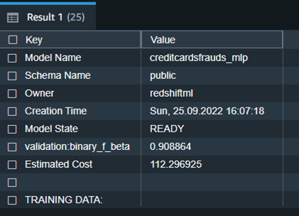
We notice from the preceding table that the F1-score for the training data is 0.908, which shows very good performance accuracy.
To elaborate, F1-score is the harmonic mean of precision and recall. It combines precision and recall into a single number using the following formula:

Where, Precision means: Of all positive predictions, how many are really positive?
And Recall means: Of all real positive cases, how many are predicted positive?
F1 scores can range from 0 to 1, with 1 representing a model that perfectly classifies each observation into the correct class and 0 representing a model that is unable to classify any observation into the correct class. So higher F1 scores are better.
The following is the detailed tabular outcome for the preceding command after model training was done.
| Model Name | creditcardsfrauds\_mlp |
| Schema Name | public |
| Owner | redshiftml |
| Creation Time | Sun, 25.09.2022 16:07:18 |
| Model State | READY |
| validation:binary\_f\_beta | 0.908864 |
| Estimated Cost | 112.296925 |
| TRAINING DATA: | . |
| Query | SELECT * FROM CREDITCARDSFRAUDS WHERE TXTIME < 120954 |
| Target Column | CLASS |
| PARAMETERS: | . |
| Model Type | mlp |
| Problem Type | BinaryClassification |
| Objective | F1 |
| AutoML Job Name | redshiftml-20221118035728881011 |
| Function Name | creditcardsfrauds\_mlp\_fn |
| . | creditcardsfrauds\_mlp\_fn\_prob |
| Function Parameters | txtime v1 v2 v3 v4 v5 v6 v7 v8 v9 v10 v11 v12 v13 v14 v15 v16 v17 v18 v19 v20 v21 v22 v23 v24 v25 v26 v27 v28 amount |
| Function Parameter Types | int4 float8 float8 float8 float8 float8 float8 float8 float8 float8 float8 float8 float8 float8 float8 float8 float8 float8 float8 float8 float8 float8 float8 float8 float8 float8 float8 float8 float8 float8 |
| IAM Role | default |
| S3 Bucket | redshift-ml-blog-mlp |
| Max Runtime | 54000 |
Redshift ML now supports Prediction Probabilities for binary classification models. For classification problem in machine learning, for a given record, each label can be associated with a probability that indicates how likely this record really belongs to the label. With option to have probabilities along with the label, customers could use the classification results when confidence based on chosen label is higher than a certain threshold value returned by the model
Prediction probabilities are calculated by default for binary classification models and an additional function is created while creating model without impacting performance of the ML model.
In above snippet, you will notice that predication probabilities enhancements have added another function as a suffix (\_prob) to model function with a name ‘creditcardsfrauds\_mlp\_fn\_prob’ which could be used to get prediction probabilities.
Additionally, you can check the model explainability to understand which inputs contributed effectively to derive the prediction.
Model explainability helps to understand the cause of prediction by answering questions such as:
- Why did the model predict a negative outcome such as blocking of credit card when someone travels to a different country and withdraws a lot of money in different currency?
- How does the model make predictions? Lots of data for credit cards can be put in a tabular format and as per MLP process where a fully connected neural network of several layers is involved, we can tell which input feature actually contributed to the model output and its magnitude.
- Why did the model make an incorrect prediction? E.g. Why is the card blocked even though the transaction is legitimate?
- Which features have the largest influence on the behavior of the model? Is it just based upon the location where the credit card is swiped, or even the time of the day and unusual credit consumption that is influencing the prediction?
Run the following SQL command to retrieve the values from the explainability report:

In the preceding screenshot, we have only selected the column that projects shapley values from the response returned by the explain\_model function. If you notice the response of the query, the values in every json object show the contribution of different features in terms of influencing the prediction. E.g. from the preceding snippet, v14 feature is influencing the prediction the most and txtime feature does not really play any significant role in predicting ‘class’.
Model validation
Now let’s run the prediction query and validate the accuracy of the model on the validation dataset:

We can observe here that Redshift ML is able to identify 99.88 percent of the transactions correctly as fraudulent or non-fraudulent.
Now you can continue to use this SQL function creditcardsfrauds\_mlp\_fn for local inference in any part of the SQL query while analyzing, visualizing or reporting the newly arriving as well as existing data!
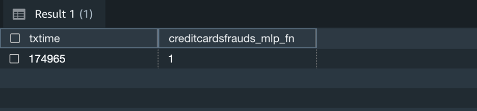
Here the output 1 means that the newly captured transaction is fraudulent as per the inference.
Additionally, you can change the above query to include prediction probabilities of label output for the above scenario and decide if you still like to use the prediction by the model.
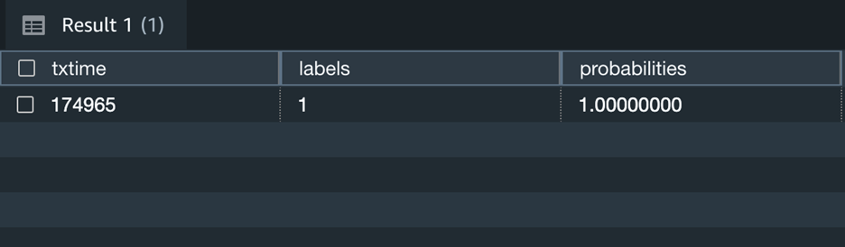
The above screenshot shows that this transaction has 100% likelihood of being fraudulent.
Clean up
To avoid incurring future charges, you can stop the Redshift cluster when not being used. You can even terminate the Redshift cluster altogether if you have run the exercise in this blog post just for experimental purpose. If you are instead using serverless version of Redshift, it will not cost you anything, until it is used. However, like mentioned before, you will have to stop or terminate the cluster if you are using a provisioned version of Redshift.
Conclusion
Redshift ML makes it easy for users of all levels to create, train, and tune models using SQL interface. In this post, we walked you through how to use the MLP algorithm to create binary classification model. You can then use those models to make predictions using simple SQL commands and gain valuable insights.
To learn more about RedShift ML, visit Amazon Redshift ML.
About the authors
 Anuradha Karlekar is a Solutions Architect at AWS working majorly for Partners and Startups. She has over 15 years of IT experience extensively in full stack development, deployment, building data ETL pipelines and visualizations. She is passionate about data analytics and text search. Outside work – She is a travel enthusiast!
 Phil Bates is a Senior Analytics Specialist Solutions Architect at AWS with over 25 years of data warehouse experience.
 Abhishek Pan is a Solutions Architect-Analytics working at AWS India. He engages with customers to define data driven strategy, provide deep dive sessions on analytics use cases & design scalable and performant Analytical applications. He has over 11 years of experience and is passionate about Databases, Analytics and solving customer problems with help of cloud solutions. An avid traveller and tries to capture world through my lenses
Debu Panda is a Senior Manager, Product Management at AWS, is an industry leader in analytics, application platform, and database technologies, and has more than 25 years of experience in the IT world. Debu has published numerous articles on analytics, enterprise Java, and databases and has presented at multiple conferences such as re:Invent, Oracle Open World, and Java One. He is lead author of the EJB 3 in Action (Manning Publications 2007, 2014) and Middleware Management (Packt).
Amazon QuickSight is a fully managed, cloud-native business intelligence (BI) service that makes it easy to connect to your data, create interactive dashboards, and share them with tens of thousands of users, either directly within a QuickSight application, or embedded in web apps and portals.
Let’s consider AnyCompany, which owns healthcare facilities across the country. The central IT team of AnyCompany is responsible for setting up and maintaining IT infrastructure and services for all the facilities in each state. Because AnyCompany is in the healthcare industry and holds sensitive data, they want to store their database credentials safely and don’t want to share them with individuals in the reporting or BI teams. Additionally, they need to encrypt their data at rest using their own encryption key instead of service-managed keys to satisfy their regulatory requirements. AnyCompany is able to audit access of their SPICE (the QuickSight robust in-memory calculation engine) datasets. In an unlikely case of a security incident, AnyCompany is in full control to immediately lock down access to their data by universally revoking access to their AWS Key Management Service (AWS KMS) keys. QuickSight is one of the services used by AnyCompany, and central IT needs to be able to set up these security measures.
QuickSight Enterprise Edition now supports storing database credentials in AWS Secrets Manager, a feature that allows you to put these credentials in Secrets Manager and not share with every BI user for data source creation. Secrets Manager is a secret storage service that you can use to protect database credentials, API keys, and other secret information. Using a key helps you ensure that the secret can’t be compromised by someone examining your code, because the secret isn’t stored in the code.
Additionally, QuickSight supports account administrators to use their own customer managed key (CMK) to encrypt and manage datasets in SPICE, through integration with AWS KMS. AWS KMS lets you create, manage, and control cryptographic keys across your applications and more than 100 AWS services. With AWS KMS, you can encrypt data across your AWS workloads, digitally sign data, encrypt within your applications using the AWS Encryption SDK, and generate and verify message authentication codes (MACs). Using a QuickSight SPICE CMK enables QuickSight users to revoke access to SPICE datasets with one click, and maintain an auditable log that tracks how SPICE datasets are accessed.
Both features help increase the level of security and transparency, give you more control over QuickSight, and help satisfy security requirements by company and government agency policies.
In this post, we walk you through the steps to use these features.
Solution overview
To enable both features (storing of database credentials in Secrets Manager and using KMS keys for encryption), we require an administrator of the QuickSight account. In the following sections, we walk you through the high-level steps to implement this solution:
- Enable Secrets Manager integration from the QuickSight management console.
- Create or update a data source with secret credentials using the QuickSight API.
- Create a dataset using the data source you created.
- Enable KMS keys from the QuickSight management console.
- Audit CMK usage and dataset access in AWS CloudTrail.
- Revoke access to CMK-encrypted datasets.
Prerequisites
Make sure you have the following prerequisites:
- A QuickSight subscription with Enterprise Edition
- A secret in Secrets Manager with your database credentials
- KMS keys to encrypt data in SPICE
Enable Secrets Manager integration
With this integration, you no longer need to manually enter data source credentials; you can store them in Secrets Manager and manage access via Secrets Manager. You can also rotate the keys and credentials in one place instead of updating all the data sources. Complete the following steps to enable the integration:
- Sign in to your QuickSight account.
- On the user name drop-down menu, choose Manage QuickSight.

- Choose Security & permissions in the navigation pane.
- Under QuickSight access to AWS services, choose Manage.

- From the list of services, choose Select secrets under AWS Secrets Manager.

- Select the appropriate secret from the list of secrets and choose Finish.

QuickSight creates an AWS Identity and Access Management (IAM) role called aws-quicksight-secretsmanager-role-v0 in your account. It grants users in the account read-only access to the specified secrets and looks similar to the following code:

Create a data source with secret credentials using the QuickSight API
At the time of this writing, creation of data sources using the stored secret in Secrets Manager is only available through the CreateDatasource public API.
The following code is an example API call to create a data source in QuickSight. This example uses the create-data-source API operation. You can also use the update-data-source operation to update an existing data source. For more information, see CreateDataSource and UpdateDataSource.
In the preceding call, QuickSight authorizes secretsmanager:GetSecretValue access to the secret based on the API caller’s IAM policy, not the IAM service role’s policy. The IAM service role acts on the account level and is used when an analysis or dashboard is viewed by a user. It can’t be used to authorize secret access when a user creates or updates the data source.
We get the following response:
In the initial response, the creation status is CREATION\_IN\_PROGRESS. To check if the data source was successfully created, use the DescribeDatasource API to receive a description of the data source:
A successful API call returns the data source object that includes status and data source details:
Create a dataset using the new data source
For instructions on creating a new SPICE dataset using the data source you just created, refer to Creating a dataset using an existing data source.
Enable KMS keys
To enable KMS keys, complete the following steps:
- On the QuickSight start page, choose Manage QuickSight.

- Choose KMS keys in the navigation pane.
- Choose Manage.

- On the KMS Keys page, choose Select key.

- In the Select key pop-up box, on the Key menu, choose the key that you want to add.

If your key isn’t on the list, you can manually enter the key’s ARN.
- Choose Use as default encryption key for all new SPICE datasets in this QuickSight account to set the selected key as your default key.
A blue badge appears next to the default key to indicate its status.
When you choose a default key, all new SPICE datasets that are created in the Region that hosts your QuickSight account are encrypted with the default key.

- Optionally, add more keys by repeating the previous steps.
Although you can add as many keys as you want, you can only have one default key at one time.
- Optionally, change or remove CMKs by changing or deleting the default key for all new SPICE datasets.
For existing datasets, you need to perform a full refresh after changing or deleting the default key to take effect.
Audit CMK usage and dataset access in CloudTrail
When a key is used (for example, when a CMK-encrypted SPICE dataset is accessed), an audit log is created in CloudTrail. You can use the log to track the key’s usage. For more information, see Logging operations with AWS CloudTrail. If you need to know which key a SPICE dataset is encrypted by, you can find this information in CloudTrail. Complete the following steps:
- On the CloudTrail console, navigate to your CloudTrail log.
- Locate the CMK usage (CMK-encrypted SPICE dataset access), using the following search arguments:
- The event name (
eventName) isGenerateDataKeyor Decrypt. - The eventTime denotes when the CMK is used (a CMK-encrypted SPICE dataset is accessed).
- The request parameters (
requestParameters) contain the QuickSight ARN for the dataset. - The request parameters (
requestParameters) contain the KMS ARN (keyId) of the CMK.
- The event name (
See the following code:
Now we can verify the CMK that’s currently used by a SPICE dataset.
- In your CloudTrail log, locate the most recent grant events for the SPICE dataset using the following search arguments:
- The event name (
eventName) contains Grant. - The request parameters (
requestParameters) contain the QuickSight ARN for the dataset.
- The event name (
See the following code:
Depending on the event type, one of the following applies:
- CreateGrant – You can find the most recently used CMK in the key ID (
keyID) for the last CreateGrant event for the SPICE dataset - RetireGrant – If latest CloudTrail event of the SPICE dataset is
RetireGrant, there is no key ID and the SPICE dataset is no longer CMK encrypted
Revoke access to CMK-encrypted datasets
You can revoke access to your CMK-encrypted SPICE datasets. When you revoke access to a key that is used to encrypt a dataset, access to the dataset is denied until you undo the revoke. The following method is one example of how you can revoke access:
- On the AWS KMS console, choose Customer managed keys in the navigation pane.
- Select the key that you want to turn off.
- On the Key actions menu, choose Disable.

After you revoke access by using any method, it can take up to 15 minutes for the SPICE dataset to become inaccessible.
Sample implementation
The following code shows a sample CreateDatasource API call for creating a QuickSight data source:
We get the following response:

To monitor the status of the new data source, run the DescribeDataSource API:
aws quicksight describe-data-source –aws-account-id <AccountId> \ –data-source-id hospitaldataASM
We get the following response:

To validate the KMS keys used, navigate to CloudTrail logs, as shown in the following code:

Finally, audit the CMK usage (dataset access) via CloudTrail logs. And in the unlikely case of a security incident, access to data can be locked down universally by revoking access to the KMS keys.
Clean up
Clean up the resources created as part of this post with the following steps:
- To remove the Secrets Manager integration, update the data source with regular service-level credentials.
- Remove the secret from the QuickSight admin console.
- On the QuickSight start page, choose Manage QuickSight.
- Choose KMS keys in the navigation pane.
- Choose Manage.
- Choose the Actions menu (three dots) on the row of the default key, then choose Delete.
- In the pop-up box that appears, choose Remove.
Conclusion
This post showcased the new features released in QuickSight to secure database credentials through integration with Secrets Manager and AWS KMS. We also demonstrated how to set up customer managed keys to enable encryption of data at rest in QuickSight SPICE, track key usage history using CloudTrail, and lock down access to data by revoking access to KMS keys.
Try out QuickSight support for Secrets Manager and AWS KMS integration to secure your credentials and data with QuickSight, and share your feedback and questions in the comments. For more information, refer to Key management and Using AWS Secrets Manager secrets instead of database credentials in Amazon QuickSight.
About the authors
Srikanth Baheti is a Specialized World Wide Sr. Solution Architect for Amazon QuickSight. He started his career as a consultant and worked for multiple private and government organizations. Later he worked for PerkinElmer Health and Sciences & eResearch Technology Inc, where he was responsible for designing and developing high traffic web applications, highly scalable and maintainable data pipelines for reporting platforms using AWS services and Serverless computing.
Raji Sivasubramaniam is a Sr. Solutions Architect at AWS, focusing on Analytics. Raji is specialized in architecting end-to-end Enterprise Data Management, Business Intelligence and Analytics solutions for Fortune 500 and Fortune 100 companies across the globe. She has in-depth experience in integrated healthcare data and analytics with wide variety of healthcare datasets including managed market, physician targeting and patient analytics.
The AWS Analytics sales team is a group of subject-matter experts who work to enable customers to become more data driven through the use of our native analytics services like Amazon Athena, Amazon Redshift, and Amazon QuickSight. Every month, each sales leader is responsible for reporting on observations and trends in their business. To support their observations, the leaders track key metrics for their region as part of their monthly business review (MBR).
Today, sales leaders use a QuickSight dashboard to analyze these key metrics. Establishing a baseline is a time-intensive process that requires navigating various tabs and filters. To save time, analytics sales managers for the Americas regions have been eager to ask QuickSight Q, in their own business language, questions like “Who are my top customers by month-over-month revenue?” or “How much did Customer X spend on Amazon Redshift this month compared with last?”
Rather than manually filtering their views to understand the underlying signals, they now use the native capabilities of QuickSight Q, resulting in many hours saved per leader.
These sales leaders can instead focus on “why it happened” and “what’s coming next” (spoiler alert: Q supports “why?” and forecast questions).
Since each leader reports on the same metrics each month, they would like to save each QuickSight Q answer, curated for their region, so they can focus on growing their business. With QuickSight Q pinboards, they can do just that. They can pin visuals for one-click access to frequently asked questions. Every time the dataset updates, the visual will reflect the latest data, all of which gets rendered in seconds because of SPICE (Super-fast, Parallel, In-memory Calculation Engine).
The features explored in this post are part of Amazon QuickSight Q. Powered by machine learning (ML), Q uses natural language processing to answer your business questions quickly. If you’re an existing QuickSight user, be sure that the Q add-on is enabled. For steps on how to do this, see Getting started with Amazon QuickSight Q.
Personalized data for sales managers
Kellie Burton, Sr. QuickSight Solutions Architect, and Amy Laresch, a Product Manager for QuickSight Q, worked with sales leaders Patrick Callahan, US West, and Jeff Pratt, US Central, to build a QuickSight Q topic for Americas Analytics revenue. A topic is a collection of one or more datasets that represents a subject area that business users can ask questions about. The Americas Analytics topic is built on a revenue dataset that is protected with row-level security (RLS), so any question asked is restricted by the same rules.
To keep the topic focused and avoid potential language ambiguity, Kellie and Amy used copies of previous MBR deliverables to understand what measures, dimensions, and calculated fields were required in the topic. With QuickSight Q automated data prep, the calculated fields were automatically added to the topic, so the topic authors did not have to recreate them. With Q, readers could ask questions like “year-to-date (YTD) YoY % for us-west analytics by segment” to get the exact table view that Patrick includes in his MBR. During a usability session, the authors worked with Jeff and Patrick to ask Q each required question and save it to their pinboard.
After opening his completed pinboard, Jeff said, “Wow, that is really cool. It answers all the questions I write the MBR for in my own custom pinboard. A report that used to take me 2-3 hours to pull together will now only take me 5 minutes.” With the extra time, he’s energized to focus more on the story behind the data and planning for future.
Patrick shared Jeff’s sentiment saying, “This will be awesome for next month when I write my MBR. What previously took a couple of hours, I can now do in a few minutes. Now I can spend more time working to deliver my customer’s outcomes.”

Sample pinboard for a sales leader for the Americas region with mock data (from the Software Sales sample topic)
Once you have an answer to a question, you might want to understand why that happened. This is where Q Why questions come into play.
Why questions
Understanding why is critical to making data-backed decisions to delight your customers and grow your business. For example, in this Software Sales sample topic, I asked Q for monthly revenue and noticed a drop in October 2022.

Mock data from the Software Sales sample topic
I ask Q, “Why?” and see four key drivers: Customer Contact, Country, Product, and Industry.
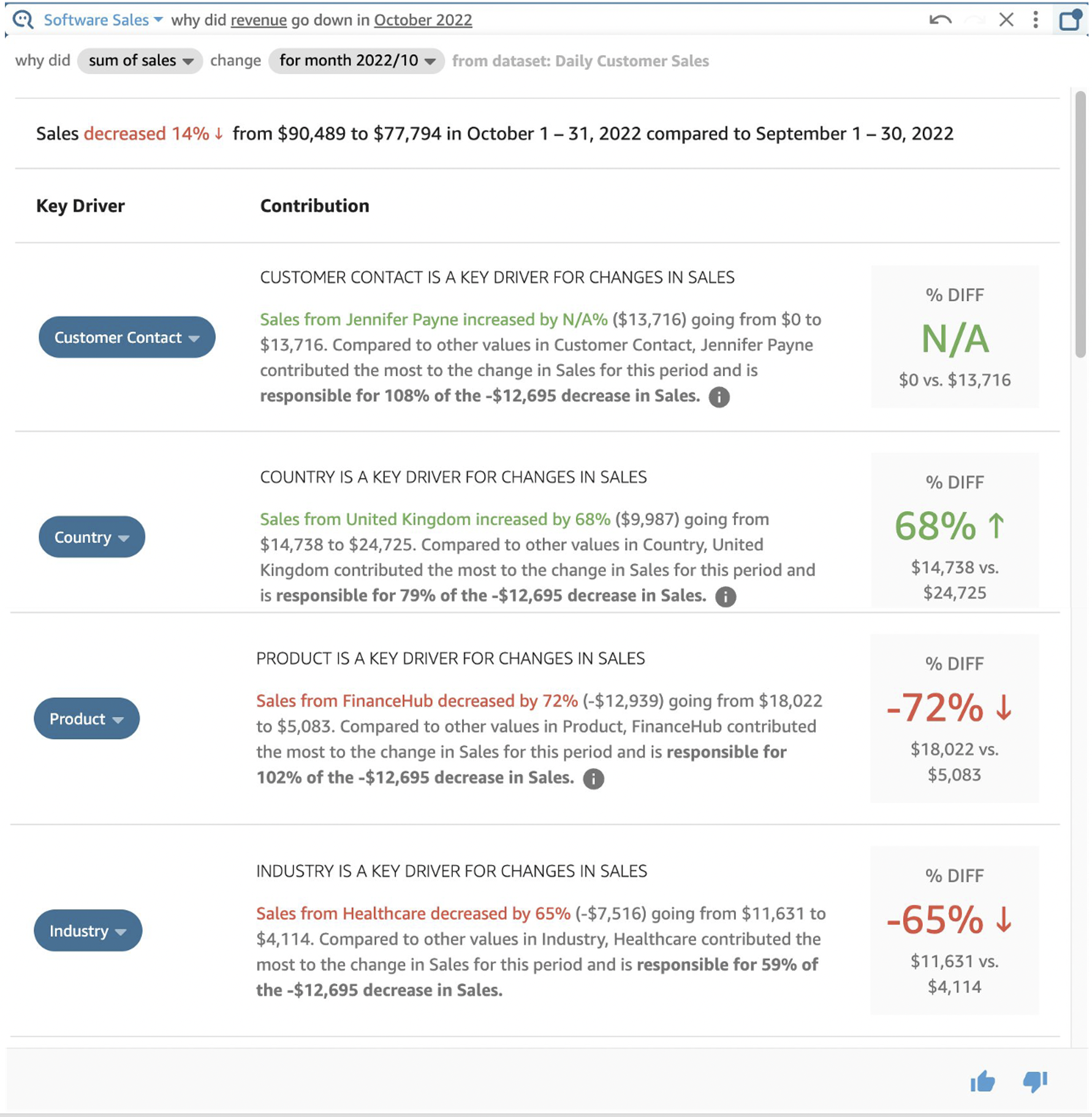
Next, I change Country to Region to see the impact at a higher level.
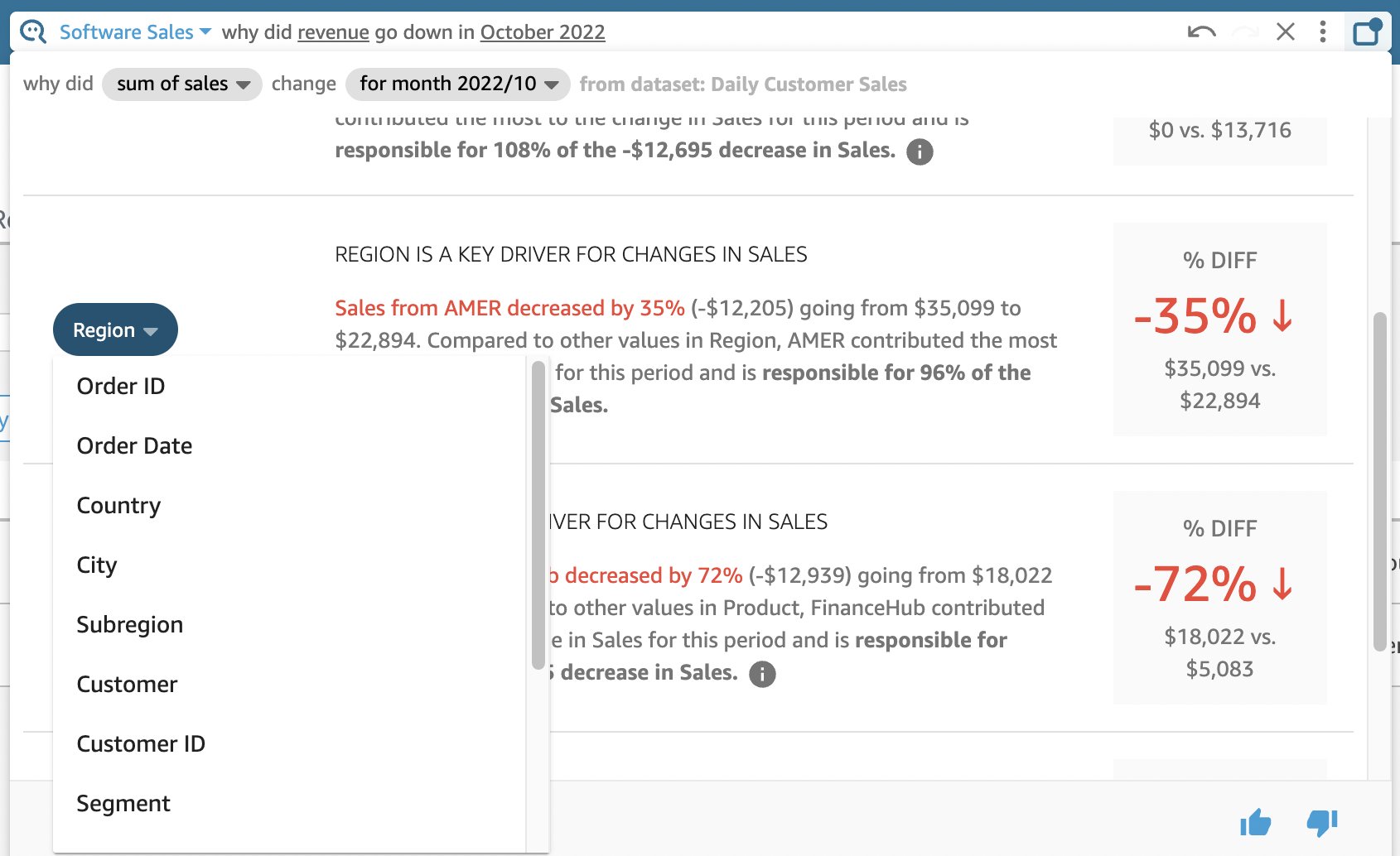
Forecast questions
Next, I can ask Q for a forecast that uses ML and factors, like seasonality, to predict the trend.

With pinboards, why questions, and forecast questions, QuickSight Q not only saves significant time and energy but delivers insights that previously required the help of an analyst or data scientist. Reflecting on the project, Kellie shared, “It’s been fun building on the bleeding edge of analytics. I’m so excited to see what Q will do in 2023!”
To learn more, watch What’s New for Readers with Amazon QuickSight Q and What’s New for Authors with Amazon QuickSight Q.
About the authors
 Amy Laresch is a product manager for Amazon QuickSight Q. She is passionate about analytics and is focused on delivering the best experience for every QuickSight Q reader. Check out her videos on the @AmazonQuickSight YouTube channel for best practices and to see what’s new for QuickSight Q.
 Kellie Burton is a Sr. Solutions Architect for Amazon QuickSight with over 25 years of experience in business analytics helping customers across a variety of industries. Kellie has a passion for helping customers harness the power of their data to uncover insights to make decisions.
Amazon EMR provides a managed service to easily run analytics applications using open-source frameworks such as Apache Spark, Hive, Presto, Trino, HBase, and Flink. The Amazon EMR runtime for Spark and Presto includes optimizations that provide over 2x performance improvements over open-source Apache Spark and Presto.
With Amazon EMR release 6.8, you can now use Amazon Elastic Compute Cloud (Amazon EC2) instances such as M6A and C6A, which use the third generation AMD EPYC processors. These instances improve the price performance of running Spark workloads on Amazon EMR by 15–50 percent over previous generation instances. In this blog post, we describe how we estimated this price performance benefit.
Amazon EMR runtime performance with EC2 M6A instances
We ran TPC-DS 3 TB benchmark queries on Amazon EMR 6.8 using Amazon EMR runtime for Apache Spark (compatible with Apache Spark 3.3) with M6a instances. Data was stored in Amazon Simple Storage Service (Amazon S3), and results were compared to equivalent clusters with M5a, which is the previous generation instance family. We measured performance improvements using the total query runtime and the geometric mean of query runtime across TPC-DS 3 TB benchmark queries.
Our results showed a 23.6–50.3 percent improvement in total query runtime performance and 22.8–52.4 percent in geometric mean on an EMR cluster with M6a compared to an equivalent EMR cluster with M5a instances. In comparing costs, we observed a 23.2–41.4 percent reduction in cost on the EMR cluster with M6a compared to the equivalent with M5a. M6A 48 XL and 32 XL instances were not benchmarked because the M5A generation does not offer equivalent sizes.
The following table shows the results from running TPC-DS 3 TB benchmark queries using Amazon EMR 6.8 over equivalent M6a and M5a instance EMR clusters.
| Instance Size | 24 XL | 16 XL | 12 XL | 8 XL | 4 XL | 2 XL | XL |
| Total size of the cluster (1 Leader + 5 core nodes) | 6 | 6 | 6 | 6 | 6 | 6 | 6 |
| Total query runtime on M5A (seconds) | 6624.1713838714 | 5466.7251180433 | 5269.0578151495 | 5366.1486275129 | 7753.6218015794 | 12118.0922180235 | 21070.6905510002 |
| Total query runtime on M6A (seconds) | 3295.2894058371 | 3063.7807673078 | 3399.1509249577 | 3482.8401591909 | 4906.2216891762 | 9184.4366036450 | 16107.9707619002 |
| Total query runtime improvement with M6A | 50.25% | 43.96% | 35.49% | 35.10% | 36.72% | 24.21% | 23.55% |
| Geometric mean query runtime M5A (sec) | 51.1422829354 | 40.9550798753 | 38.4890223194 | 35.3863834186 | 44.8454957416 | 61.0454658020 | 92.6414502105 |
| Geometric mean query runtime M6A (sec) | 24.3406154481 | 22.3484713891 | 22.9913163520 | 23.0351017440 | 28.2855683398 | 46.4363267349 | 71.5498816854 |
| Geometric mean query runtime improvement with M6A | 52.41% | 45.43% | 40.27% | 34.90% | 36.93% | 23.93% | 22.77% |
| EC2 M5A instance price ($ per hour) | $4.12800 | $2.75200 | $2.06400 | $1.37600 | $0.68800 | $0.34400 | $0.17200 |
| EMR M5A instance price ($ per hour) | $0.27000 | $0.27000 | $0.27000 | $0.27000 | $0.17200 | $0.08600 | $0.04300 |
| (EC2 + EMR) M5A instance price ($ per hour) | $4.39800 | $3.02200 | $2.33400 | $1.64600 | $0.86000 | $0.43000 | $0.21500 |
| Cost of running on M5A ($ per instance) | $8.09253 | $4.58901 | $3.41611 | $2.45352 | $1.85225 | $1.44744 | $1.25839 |
| EC2 M6A instance price ($ per hour) | $4.14720 | $2.76480 | $2.07360 | $1.38240 | $0.69120 | $0.34560 | $0.17280 |
| EMR M6A price ($ per hour per instance) | $1.03680 | $0.69120 | $0.51840 | $0.34560 | $0.17280 | $0.08640 | $0.04320 |
| (EC2 + EMR) M6A instance price ($ per hour) | $5.18400 | $3.45600 | $2.59200 | $1.72800 | $0.86400 | $0.43200 | $0.21600 |
| Cost of running on M6A ($ per instance) | $4.74522 | $2.94123 | $2.44739 | $1.67176 | $1.17749 | $1.10213 | $0.96648 |
| Total cost reduction with M6A including performance improvement | -41.36% | -35.91% | -28.36% | -31.86% | -36.43% | -23.86% | -23.20% |
The following graph shows per query improvements observed on M6a 2XL instances compared to equivalent M5a generation. We observed that two queries take longer to execute on M6a instance clusters compared to M5a instance clusters. Q91 regressed up to 6.64 percent and Q55 regressed up to 1.86 percent on 4 XL instance clusters.

Amazon EMR runtime performance with EC2 R6A instances
R6A instances showed a similar performance improvement while running Apache Spark workloads compared to equivalent R5A instances. R6A 32XL and 48XL instances were not benchmarked since R5A instances do not have 32XL and 48XL sizes available. Our results showed 16–58.22 percent improvement in total query runtime for seven different instance sizes within the instance family and 20.04–59.59 percent improvement in geometric mean. In comparing costs, we observed 15.85–-50.07 percent reduction in cost on R6A instance EMR clusters compared to R5A EMR instance clusters.
The following table shows the results from running TPC-DS 3 TB benchmark queries using Amazon EMR 6.8 over equivalent R6A and R5A instance EMR clusters.
| Instance Size | 24 XL | 16 XL | 12 XL | 8 XL | 4 XL | 2 XL | XL |
| Total size of the cluster (1 Leader + 5 core nodes) | 6 | 6 | 6 | 6 | 6 | 6 | 6 |
| Total query runtime on R5A (seconds) | 6934.22936 | 5530.74672 | 5834.32344 | 5718.72582 | 7615.58392 | 11431.37368 | 20688.58642 |
| Total query runtime on R6A (seconds) | 2897.44817 | 2906.49952 | 3017.85315 | 3488.83875 | 4661.32856 | 7717.33575 | 17378.49043 |
| Total query runtime improvement with R6A | 58.22% | 47.45% | 48.27% | 38.99% | 38.79% | 32.49% | 16.00% |
| Geometric mean query runtime R5A (sec) | 53.27574 | 41.76973 | 42.50324 | 37.62155 | 44.58173 | 58.88182 | 91.72095 |
| Geometric mean query runtime R6A (sec) | 21.52803 | 21.36831 | 19.94607 | 21.59493 | 26.90097 | 36.57557 | 73.3405 |
| Geometric mean query runtime improvement with R6A | 59.59% | 48.84% | 53.07% | 42.60% | 39.66% | 37.88% | 20.04% |
| EC2 R5A instance price ($ per hour) | $5.42400 | $3.61600 | $2.71200 | $1.80800 | $0.90400 | $0.45200 | $0.22600 |
| EMR R5A instance price ($ per hour) | $0.27000 | $0.27000 | $0.27000 | $0.27000 | $0.22600 | $0.11300 | $0.05700 |
| (EC2 + EMR) R5A instance price ($ per hour) | $5.69400 | $3.88600 | $2.98200 | $2.07800 | $1.13000 | $0.56500 | $0.28300 |
| Cost of running on R5A ($ per instance) | $10.96764 | $5.97013 | $4.83276 | $3.30098 | $2.39045 | $1.79409 | $1.62635 |
| EC2 R6A instance price ($ per hour) | $5.44320 | $3.62880 | $2.72160 | $1.81440 | $0.90720 | $0.45360 | $0.22680 |
| EMR R6A price ($ per hour per instance) | $1.36080 | $0.90720 | $0.68040 | $0.45360 | $0.22680 | $0.11340 | $0.05670 |
| (EC2 + EMR) R6A instance price ($ per hour) | $6.80400 | $4.53600 | $3.40200 | $2.26800 | $1.13400 | $0.56700 | $0.28350 |
| Cost of running on R6A ($ per instance) | $5.47618 | $3.66219 | $2.85187 | $2.19797 | $1.46832 | $1.21548 | $1.36856 |
| Total cost reduction with R6A including performance improvement | -50.07% | -38.66% | -40.99% | -33.41% | -38.58% | -32.25% | -15.85% |
Benchmarking methodology
The benchmark used in this post is derived from the industry-standard TPC-DS benchmark and uses queries from the Spark SQL Performance Tests GitHub repo with the following fixes applied.
We calculated TCO by multiplying cost per hour by number of instances in the cluster and time taken to run the queries on the cluster. We used the on-demand pricing in the US East (N. Virginia) Region for all instances.
Conclusion
In this post, we described how we estimated the cost-performance benefit from using Amazon EMR with M6A and R6A instances compared to using equivalent previous-generation instances. Using these new instances with Amazon EMR improves price performance by 15–50%.
About the authors
Al MS is a product manager for Amazon EMR at Amazon Web Services.
Kyeonghyun Ryoo is a Software Development Engineer for EMR at Amazon Web Services. He primarily works on designing and building automation tools for internal teams and customers to maximize their productivity. Outside of work, he is a retired world champion in professional gaming who still enjoy playing video games.
Amazon OpenSearch Service makes it easy for you to perform interactive log analytics, real-time application monitoring, website search, and more. Amazon OpenSearch is an open source, distributed search and analytics suite. Amazon OpenSearch Service offers the latest versions of OpenSearch, support for 19 versions of Elasticsearch (1.5 to 7.10 versions), as well as visualization capabilities powered by OpenSearch Dashboards and Kibana (1.5 to 7.10 versions). Amazon OpenSearch Service currently has tens of thousands of active customers with hundreds of thousands of clusters under management processing trillions of requests per month.
To meet the needs of customers who want simplicity in their network setup with the Amazon OpenSearch Service, you can now use Amazon OpenSearch Service-managed virtual private cloud (VPC) endpoints (powered by AWS PrivateLink) to connect to your applications using Amazon OpenSearch Service domains launched in Amazon Virtual Private Cloud (VPC). With Amazon OpenSearch Service-managed VPC endpoints, you can privately access your Amazon OpenSearch Service domain from multiple VPCs in your account or other AWS accounts based on your application needs without configuring other services features such as VPC peering, AWS Transit Gateway (TGW), or other more complex network routing strategies that place operational burden on your support and engineering teams.
The feature is built using AWS PrivateLink. AWS PrivateLink provides private connectivity between VPCs, supported AWS services, and your on-premises networks without exposing your traffic to the public internet. It provides you with the means to connect multiple application deployments effortlessly to your Amazon OpenSearch Service domains.
This post introduces Amazon OpenSearch Service-managed VPC endpoints that build on top of AWS PrivateLink and shows how you can access a private Amazon OpenSearch Service from one or more VPCs hosted in the same account, or even VPCs hosted in other AWS accounts using AWS PrivateLink managed by Amazon OpenSearch Service.
Amazon OpenSearch Service managed VPC endpoints
Before the launch of Amazon OpenSearch Service managed VPC endpoints, if you needed to gain access to your domain outside of your VPC, you had three options:
- Use VPC peering to connect your VPC with other VPCs
- Use AWS Transit Gateway to connect your VPC with other VPCs
- Create your own implementation of an AWS PrivateLink setup
The first two options require you to setup your VPCs so that the Classless Inter-Domain Routing (CIDR) block ranges don’t overlap. If they did, then your options are more complicated. The third option, create your own implementation of AWS PrivateLink, involve configuring a network load balancer (NLB) and associating a target group with the NLB as one of the steps in the setup. The architecture discussed in this post, demonstrates these additional layers of complexity.
With Amazon OpenSearch Service managed VPC endpoints (i.e., powered by AWS PrivateLink), these complex setups and processes are no longer needed!
You can access your Amazon OpenSearch Service private domain as if it were deployed in all the VPCs that you want to connect to your domain. If you need private connectivity from your on-premises hybrid deployments, then AWS PrivateLink helps you bring access from your Amazon OpenSearch Service domain to your data centers with minimal effort.
By using AWS PrivateLink with Amazon OpenSearch Service, you can realize the following benefits:
- You simplify your network architecture between hybrid, multi-VPC, and multi account solutions
- You address a multitude of compliance concerns by better controlling the traffic that moves between your solutions and Amazon OpenSearch Service domains
Shared search cluster for multiple development teams
Imagine that your company hosts a service as a software (SaaS) application that provides a search application programming interface (API) for the healthcare industry. Each team works on a different function of the API. The development teams API team 1 and API team 2 are in two different AWS accounts and each has their own VPCs within these accounts. Another team (data refinement team) works on the ingestion and data refinement to populate the Amazon OpenSearch Service domain hosted in the same account as API team 2 but in different VPC. Each team shares the domain during the development cycles to save costs and foster collaboration on the data modeling.
Solution overview
Self-managed AWS PrivateLink architecture to connect different VPCs
In this scenario prior to Amazon OpenSearch Service manage VPC endpoints (i.e., powered by AWS PrivateLink), you would have to create the following items:
- Deploy an NLB in your VPC
- Create a target group that points to the IP addresses of the Elastic Network Interfaces (ENIs), which the Amazon OpenSearch Service creates in your VPC and is used to launch the Amazon OpenSearch Service
- Create an AWS PrivateLink deployment and reference your newly created NLB
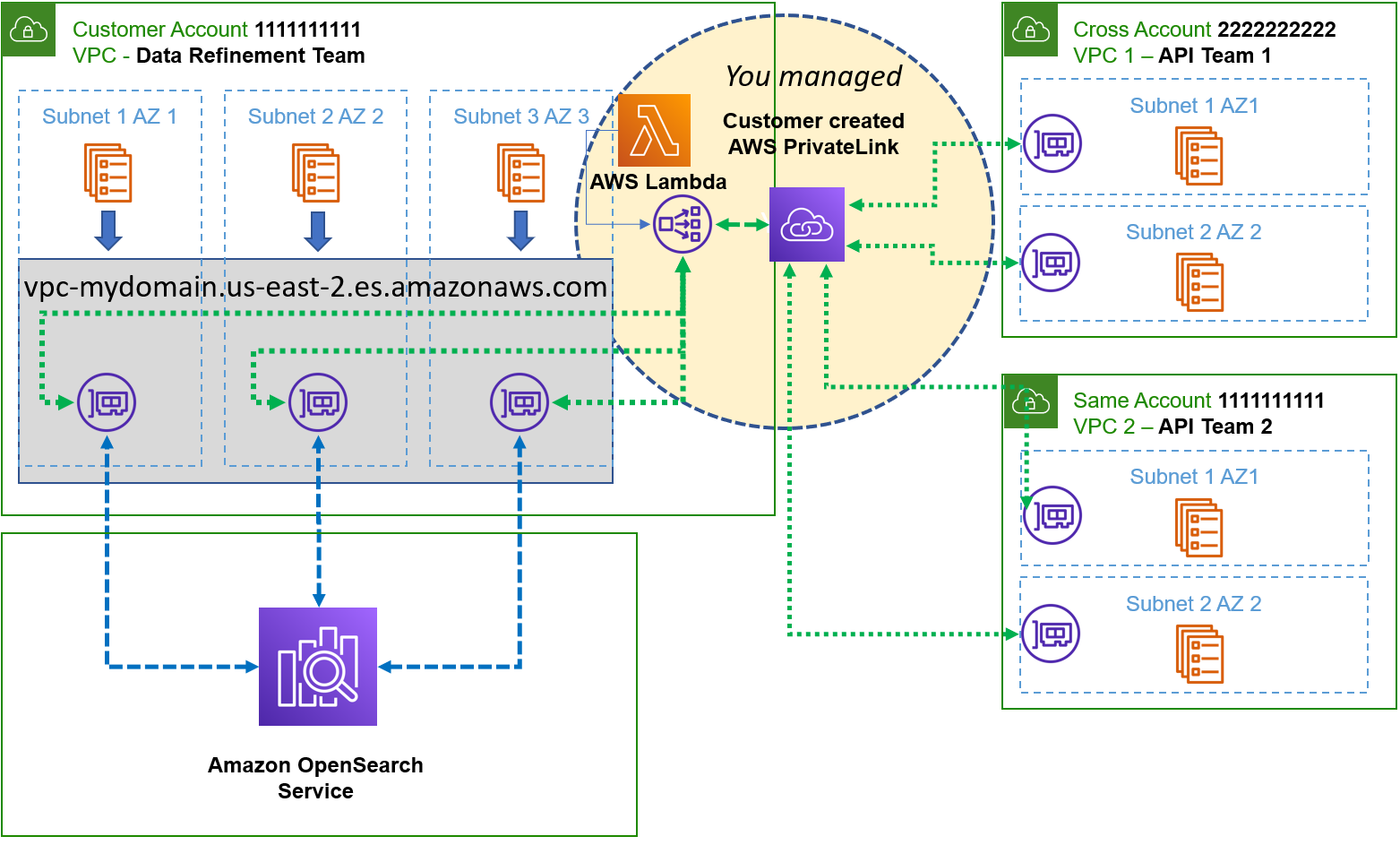
When you implement the NLB, a target group can only reference IP addresses, an Amazon EC2 instance, or an Application Load Balancer (ALB). If you referenced the IP addresses as targets, then you had to build a process that detected the changes in the IP address if the domain changed due to service initiated or self-initiated blue/green deployments. You must maintain yet another complex process to ensure that you always have active ENIs with which to point your target groups or you lose connectivity.
Typically, customers use an AWS Lambda with scheduled events in Amazon CloudWatch. This means that you use the AWS Lambda to detect the current state where the ENIs that provided the IP addresses were marked as active for the description that matched the ENIs your domain creates. You schedule AWS Lambda to wake up within the time to live (TTL) of the Domain Name Service (DNS) settings (typically 60 seconds) and compare the existing IP addresses in the target group with any new ones found when you query all ENIs with a description referencing your domain in the VPC. You then build a new target group with the deltas and you swap the target groups and drop the old one. It’s tricky, it’s complex, and you have to maintain the solution!
With the new simplified networking architecture, your teams go through the following steps.
OpenSearch Service managed VPC endpoints architecture (powered by AWS PrivateLink)
Since the Amazon OpenSearch Service takes care of the infrastructure described previously — but not necessarily on the same implementation — all you really need to concern yourself with is creating the connections using the instructions in our service documentation.
Once you complete the steps in the instructions and remove your own implementation, your architecture is then simplified as seen in the following diagram.
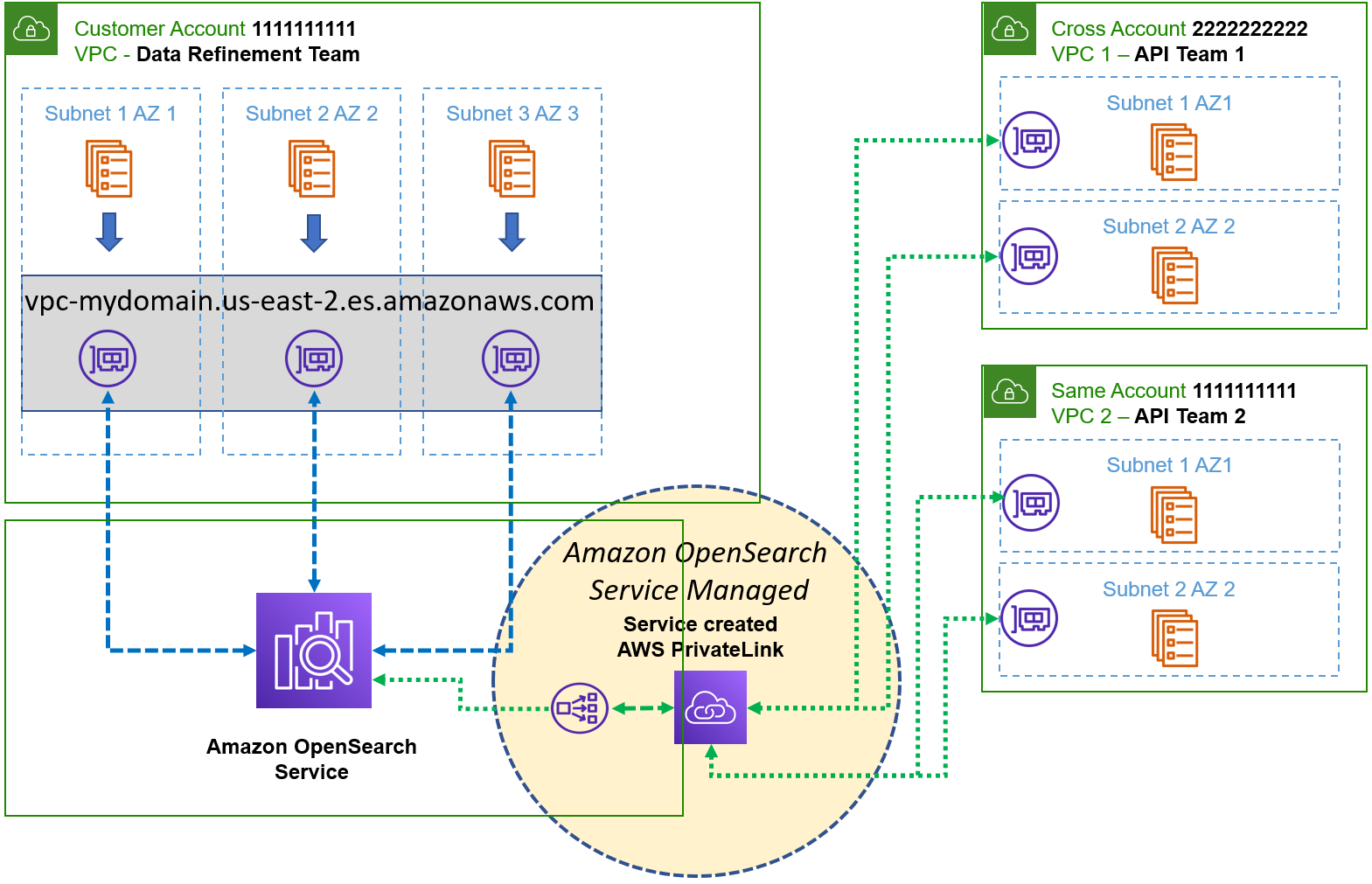
At this point, the development teams (API team 1 and API team 2) can access the Amazon OpenSearch cluster via Amazon OpenSearch Service Managed VPC Endpoint. This option is highly scalable with a simplified network architecture in which you don’t have to worry about managing a NLB, or setting up target groups and the additional resources. If the number of development teams and VPCs grow in the future, you associate the domain with the associated interface VPC endpoint. You can access services in VPCs in same or different accounts, even if there are overlapping CIDR Block IP ranges.
Conclusion
In this post, we walked through the architectural design of accessing Amazon OpenSearch cluster from different VPCs across different accounts using OpenSearch Service-managed VPC endpoint (AWS PrivateLink). Using Transit Gateway, self-managed AWS PrivateLink or VPC peering required complex networking strategies that increased operation burden. With the introduction of VPC endpoints for Amazon OpenSearch Service, the complexity of your solutions is greatly simplified and what’s even better, it’s managed for you!
About the authors
Aish Gunasekar is a Specialist Solutions architect with a focus on Amazon OpenSearch Service. Her passion at AWS is to help customers design highly scalable architectures and help them in their cloud adoption journey. Outside of work, she enjoys hiking and baking.
Kevin Fallis (@AWSCodeWarrior) is an AWS specialist search solutions architect. His passion at AWS is to help customers leverage the correct mix of AWS services to achieve success for their business goals. His after-work activities include family, DIY projects, carpentry, playing drums, and all things music.
Amazon Redshift is a fast, fully managed, petabyte-scale cloud data warehouse that enables you to analyze large datasets using standard SQL. The concurrency scaling feature in Amazon Redshift automatically adds and removes capacity by adding concurrency scaling to handle demands from thousands of concurrent users, thereby providing consistent SLAs for unpredictable and spiky workloads such as BI reports, dashboards, and other analytics workloads.
Until now, concurrency scaling only supported auto scaling for read queries; write queries had to run on the main cluster. Now, we are extending concurrency scaling to support auto scaling for common write queries including COPY, INSERT, UPDATE, and DELETE. This is available on Amazon Redshift RA3 provisioned instance types in the Regions where concurrency scaling is available. Amazon Redshift serverless comes with built in dynamic auto scaling capability for read workload scaling.
In this post, we discuss how to enable concurrency scaling to offer consistent SLAs for concurrent workloads such as data loads, ETL (extract, transform, and load), and data processing with reduced queue times.
Concurrency scaling overview
With concurrency scaling, Amazon Redshift automatically and elastically scales query processing power to provide consistently fast performance for hundreds of concurrent queries. Concurrency scaling resources are added to your Amazon Redshift cluster transparently in seconds, as concurrency increases, to serve sudden spikes in concurrent requests with fast performance without wait time. When the workload demand subsides, Amazon Redshift automatically shuts down concurrency scaling resources to save you cost.
The following diagram shows how concurrency scaling works at a high level.
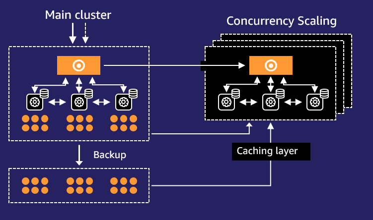
The workflow contains the following steps:
- All queries go to the main cluster.
- When queries in the designated workload management (WLM) queue begin queuing, Amazon Redshift automatically routes eligible queries to the new clusters, enabling concurrency scaling.
- Amazon Redshift automatically spins up a new cluster, processes waiting queries, and shuts down the concurrency scaling cluster when no longer needed.
Enable Amazon Redshift concurrency scaling
You can manage concurrency scaling at the WLM queue level, where you set concurrency scaling policies for specific queues. When concurrency scaling is enabled for a queue, eligible write and read queries are sent to concurrency scaling clusters without having to wait for resources to free up on the main Amazon Redshift cluster. Amazon Redshift handles spinning up concurrency scaling clusters, routing of the queries to the transient clusters, and relinquishing the concurrency clusters.
You can enable concurrency scaling on both automatic and manual WLM.
You first need to determine which parameter group your cluster is. To do so, complete the following steps:
- On the Amazon Redshift console, choose Clusters in the navigation pane.
- Choose your cluster.

- On the Properties tab, note the parameter group associated to the cluster.
 Now you can configure your WLM parameters.
 - Under Configurations in the navigation pane, choose Workload management.
- Choose the parameter group associated to the cluster.If you’re using the default parameter group default.redshift-1.0, you need to create a custom parameter group and assign that to the cluster. The default parameter group has preset values for each of its parameters, and it can’t be modified.
- On the Parameters tab, you can choose between 1–10
max\_concurrency\_scaling\_clusters.This is the max number of concurrent Amazon Redshift clusters you can have running at the same time. Ten is the soft limit; this limit can be increased by submitting a service limit increase request with a support case.
- On the Workload management tab, choose auto mode for the concurrency scaling cluster.
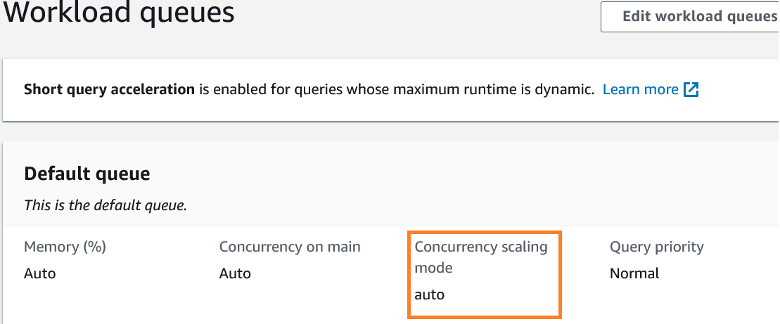
Example use cases
In this section, we use three use cases to help you understand how concurrency scaling for read and write heavy workloads can seamlessly scale to improve workload performance SLAs.
We used a 3 TB Cloud DW benchmark dataset. The test included a total of 103 concurrent queries, with each run using a separate database connection. The 103 queries constituted 60 queries from the 99 TPC-DS queries and 43 write queries, with a mix of copy, insert, update and delete statements. We used RA3.4xlarge 5 compute nodes.
The following scenarios showcase how concurrency scaling for reads and writes can seamlessly auto scale and positively impact a heavy concurrent mixed workload:
- All queries triggered concurrently with concurrency scaling turned off
- All queries triggered concurrently with concurrency scaling cluster limit set to 5 clusters
- All queries triggered concurrently with concurrency scaling cluster limit set to 10 clusters
Scenario 1: All queries triggered concurrently with concurrency scaling turned off
In this benchmark test, all queries completed in 299 minutes. The following are the test details.
The Amazon Redshift query optimizer turned the 103 queries into 257 sub-queries for better performance in this run. Amazon Redshift continuous to learn from operational statistics to optimize your workload.
The following screenshot shows how Amazon Redshift auto WLM mode chose to run 16 queries concurrently while queuing the rest. Because concurrency scaling is turned off, no additional clusters are spun up and the queries continue to wait for running queries to complete before they can be processed. Notice the number of queries queued stayed at a higher number for a long period of time and eventually lowered as only a few queries could concurrently run.

No additional concurrent clusters spun up during the window of the workload, as seen in the following screenshot, requiring the primary cluster to process all the queries.

Scenario 2: All queries triggered concurrently with concurrency scaling cluster max limit set to 5 clusters
In this test, all queries completed in 49 minutes.
The following screenshot depicts significant queuing. Within seconds, five additional Amazon Redshift clusters are spun up into ready state, allowing 53 queries to run simultaneously. This number can change in your cluster based on the query types. Notice the number of queries queued starts lowering as more queries are completed using the five additional clusters.
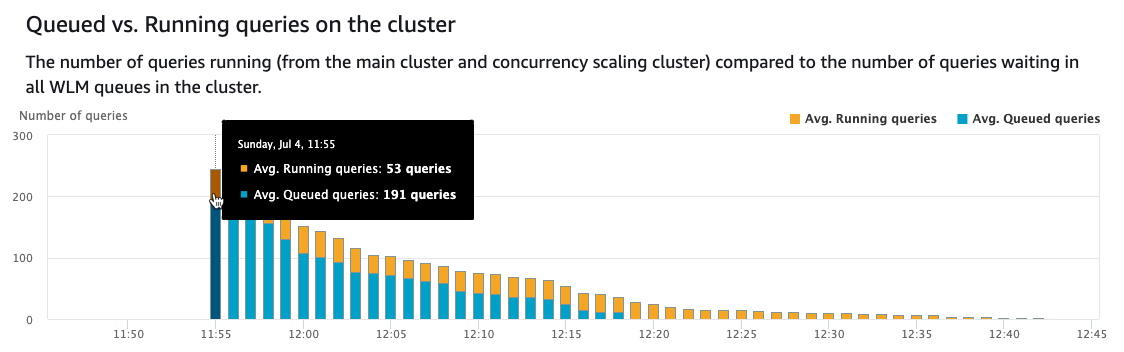
Over time, the concurrency scaling clusters start to wind down progressively to 0 as the queries no longer waited.

Scenario 3: All queries triggered concurrently with concurrency scaling cluster limit set to 10 clusters
In this test, all queries completed in 28 minutes.
The following screenshot depicts significant queuing. Within seconds, 10 additional Amazon Redshift clusters are spun up into ready state, allowing multiple queries to run simultaneously. This number can change in your cluster based on the query types. Notice the number of queries queued starts lowering as more queries are completed using the five additional clusters.

Over time, the concurrency scaling clusters start to wind down progressively to 0 as the queries no longer waited.
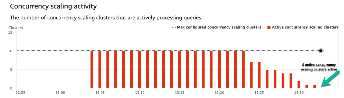
Test results review
The following table summarizes our test results.
| . | Test Scenario 1 | Test Scenario 2 | Test Scenario 3 |
| Total Workload Completion Time | 299 Minutes | 49 Minutes | 28 Minutes |
The test results reveal how concurrency scaling for a mixed workload of reads and writes lowered the total workload completion time from 299 minutes to 28 minutes, which is more than 10 times an improvement in SLAs while being cost effective by only paying for the additional clusters when scaling is necessary.
Monitor concurrency scaling
One method to monitor concurrency scaling is via system views. To monitor which queries benefitted from concurrency scaling, you can use concurrency\_scaling\_status from stl\_query. Concurrency scaling of 1 indicates that the query ran on a concurrency scaling cluster. To monitor concurrency scaling usage, you can use the SVCS\_CONCURRENCY\_SCALING\_USAGE system view.
The Amazon CloudWatch metrics ConcurrencyScalingActiveClusters and ConcurrencyScalingSeconds enable you to set up monitoring of concurrency scaling usage. For more information, refer to Monitoring Amazon Redshift using CloudWatch metrics.
Configure usage limit
With every 24 hours used of the main Amazon Redshift cluster, you accrue 1 hour of concurrency scaling credit. This free credit can be used by both read and write queries. For any usage that exceeds the accrued free usage credits, you’re billed on a per-second basis based on the on-demand rate of your Amazon Redshift cluster. You can apply cost controls for concurrency scaling at the cluster level. You can choose to create multiple queues for ETL, Dashboard, and adhoc workload. With this you can choose to turn on concurrency scaling for selective queues.
As shown in the following screenshot, you can choose a time period (daily, weekly, or monthly) and specify the desired usage limit. You can then choose an action option (Alert, Log to system table, or Disable feature). For more details on how to set cost controls for concurrency scaling, refer to Manage and control your cost with Amazon Redshift Concurrency Scaling and Spectrum.

Summary
In this post, we showed how you can enable concurrency scaling to help you meet the SLAs for both read and write workloads by seamlessly scaling out to the maximum number of clusters you configured, thereby increasing your cluster throughput while controlling your costs. Concurrency scaling with read and write capability can enable you to handle a number of scenarios, such as sudden increases in the volume of data in your data pipeline, backfill operations, ad hoc reporting, and month end processing. It’s now time to put this learning into action and begin optimizing your Redshift cluster(s) for both read and write throughput!
About the Authors
 Harsha Tadiparthi is a specialist Principal Solutions Architect, Analytics at AWS. He enjoys solving complex customer problems in databases and analytics and delivering successful outcomes. Outside of work, he loves to spend time with his family, watch movies, and travel whenever possible.
 Harshida Patel is a Specialist Principal Solutions Architect, Analytics with AWS.
 Ramu Ponugumati is a Sr. Technical Account Manager, specialist in Analytics and AI/ML at AWS. He works with enterprise customers to modernize and cost optimize workloads, and helps them build reliable and secure applications on the AWS platform. Outside of work, he loves spending time with his family, playing tennis, and gardening.
In this third post of a multi-part series, we explore some of the edge cases in migrating a large data warehouse from Greenplum to Amazon Redshift using AWS Schema Conversion Tool (AWS SCT) and how to handle these challenges. Challenges include how best to use virtual partitioning, edge cases for numeric and character fields, and arrays.
You can check out the first post of this series for guidance on planning, running, and validating the migration. You can also check out the second post for best practices for choosing the optimal Amazon Redshift cluster, data architecture, converting stored procedures, compatible functions and queries widely used for SQL conversions, and recommendations for optimizing the length of data types for table columns.
Unbounded character data type
Greenplum supports creating columns as text and varchar without specifying the length of the field. This works without an issue in Greenplum but doesn’t work well in migrating to Amazon Redshift. Amazon Redshift stores data in columnar format and gets better compression when using shorter column lengths. Therefore, the Amazon Redshift best practice is to use the smallest character length possible.
AWS SCT will convert these unbounded fields as large objects (LOBs) instead of treating the columns as character fields with a specified length. LOBs are implemented differently in each database product on the market, but in general, a LOB is not stored with the rest of the table data. Instead, there is a pointer to the location of the data. When the LOB is queried, the database reconstitutes the data automatically for you, but this typically requires more resources.
Amazon Redshift doesn’t support LOBs, so AWS SCT resolves this by loading the data into Amazon Simple Storage Service (Amazon S3) and in the column, it stores the S3 URL. When you need to retrieve this data, you have to query the table, get the S3 URL, and then fetch the data from Amazon S3. This isn’t ideal because most of the time, the actual maximum length of the field doesn’t require it to be treated as a LOB, and storing the data remotely means it will take much longer to fetch the data for queries.
The current resolution is to calculate the maximum length of these columns and update the Greenplum tables before converting to Amazon Redshift with AWS SCT.
Note that in a future release of AWS SCT, the collection of statistics will include calculating the maximum length for each column, and the conversion of unbounded varchar and text will set the length in Amazon Redshift automatically.
The following code is an example of an unbounded character data type:
This table uses a primary key column on an unbounded text column. This needs to be converted to varchar(n), where n is the maximum length found in this column.
- Drop unique constraints on affected columns:
- Drop indexes on affected columns:
- Calculate maximum length of affected columns:
Note that in this example, the description1 and description2 columns only contain NULL values, or the table doesn’t have any data in it, or the calculated length of the columns is 10.
- Alter the length of the affected columns:
You can now proceed with using AWS SCT to convert the Greenplum schema to Amazon Redshift and avoiding using LOBs to store the column values.
GitHub help
If you have many tables to update and want an automated solution, you can use the add\_varchar\_lengths.sh script found in the GitHub repo to fix all of the unbounded varchar and text columns in a given schema in Greenplum. The script calculates the appropriate maximum length and then alters the Greenplum tables so the varchar data type is bounded by a length.
Please note that the script also will drop any constraints or indexes on the affected columns.
Empty character data
Greenplum and Amazon Redshift support an empty string value in a field that is different from NULL. The behavior is the same between the two databases. However, AWS SCT defaults to convert empty strings to NULL. This simply needs to be disabled to avoid problems.
- In AWS SCT, open your project, choose Settings, Project settings, and Data migration.
- Scroll to the bottom and find Use empty as null value.
- Deselect this so that AWS SCT doesn’t convert empty strings to NULL.
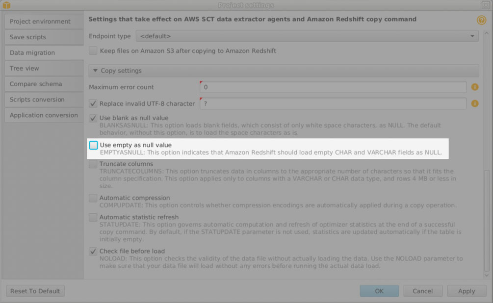
NaN and Infinity numeric data type
Greenplum supports NaN and Infinity in a numeric field to represent an undefined calculation result and infinity. NaN is very uncommon because when using aggregate functions on a column with a NaN row, the result will also be NaN. Infinity is also uncommon and not useful when aggregating data. However, you may encounter these values in a Greenplum database.
Amazon Redshift doesn’t support NaN and Infinity, and AWS SCT doesn’t check for this in your data. If you do encounter this when using AWS SCT, the task will fail with a numeric conversion error.
To resolve this, it’s suggested to use NULL instead of NaN and Infinity. This allows you to aggregate data and get results other than NaN and, importantly, allow you to convert the Greenplum data to Amazon Redshift.
The following code is an example NaN numeric value:
- Drop the NOT NULL constraint:
- Update the table:
You can now proceed with using AWS SCT to migrate the Greenplum data to Amazon Redshift.
Note that in a future release of AWS SCT, there will be an option to convert NaN and Infinity to NULL so that you won’t have to update your Greenplum data to migrate to Amazon Redshift.
Virtual partitioning on GP\_SEGMENT\_ID
For large tables, it’s recommended to use virtual partitioning to extract data from Greenplum. Without virtual partitioning, AWS SCT will run a single query to unload data from Greenplum. For example:
If this table is very large, it will take a long time to extract the data because this is a single process querying the data. With virtual partitioning, multiple queries are run in parallel so that the extraction of data is completed faster. It also makes it easier to recover if there is an issue with the task.
Virtual partitioning is very flexible, but a simple way to do this in Amazon Redshift is to utilize the Greenplum hidden column gp\_segment\_id. This column identifies which segment in Greenplum has the data, and each segment should have an equal number of rows. Therefore, creating partitions for each gp\_segment\_id is an easy way to implement virtual partitioning.
If you’re not familiar with the term segment, it’s similar to an Amazon Redshift slice.
For example:
- First, determine the number of segments in Greenplum:
Now you can configure AWS SCT.
- In AWS SCT, go to Data Migration view (other) and choose (right-click) a large table.
- Scroll down to Add virtual partitioning.
- For the partition type, choose Auto Split and change the column name to
GP\_SEGMENT\_ID. - Use
0for Start value, the number of segments found in Step 1 as End value, and Interval of1.
When you create a local task to load this table, the task will have a sub-task for each gp\_segment\_id value.
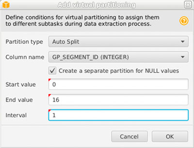
Note that in a future release of AWS SCT, there will be an option to automatically virtually partition tables based on GP\_SEGMENT\_ID. This option will also retrieve the number of segments automatically.
Arrays
Greenplum supports arrays such as bigint[] that are unbounded. Typically, arrays are kept relatively small in Greenplum because arrays consume more memory in Greenplum than using an alternative strategy. However, it’s possible to have a very large array in Greenplum that isn’t supported by Amazon Redshift.
AWS SCT converts a Greenplum array to varchar(65535), but if the converted array is longer than 65,535 characters, then the load will fail.
The following code is an example of a large array:
In this example, the sales items are stored in an array for each sales\_id. If you encounter an error while loading that the length is too long to load this data into Amazon Redshift with AWS SCT, then this is the solution. It’s also a more efficient pattern to store data in both Greenplum and Amazon Redshift!
- Create a new sales table that has all columns from the existing sales table, but exclude the array column:
- Populate the new sales table with the existing data except for the array column:
We create a new table that is a cross-reference of sales IDs with the sales items. Instead of having a single row for this association, now there will be a row for each relationship.
- Create a new sales item table:
- To unnest the array, create a row for each array element:
- Rename the sales tables:
In AWS SCT, refresh the tables and migrate the revised sales and the new sales\_items table.
The following are some example queries before and after.
Before:
After:
Before:
After:
VACUUM ANALYZE
Greenplum, like Amazon Redshift, supports the VACUUM command, which reclaims storage space after UPDATE and DELETE commands are run on a table. Greenplum also allows you to add the ANALYZE option to run both statements with a single command.
The following code is the Greenplum command:
This is not very common, but you’ll see this from time to time. If you’re just inserting data into a table, there is no need to run VACUUM, but for ease of use, sometimes developers will use VACUUM ANALYZE.
The following are the Amazon Redshift commands:
Amazon Redshift doesn’t support adding ANALYZE to the VACUUM command, so instead, this needs to be two different statements. Also note that Amazon Redshift performs VACUUM and ANALYZE automatically for you so in most cases, you can remove these commands from your scripts entirely.
DISTINCT ON query
Greenplum supports an unusual shortcut for eliminating duplicates in a table. This feature keeps the first row for each set of rows based on the order of the data being fetched. It’s easiest to understand by looking at an example:
We get the following results:
The solution for running this in Amazon Redshift is to use the ANSI standard row\_number() analytical function, as shown in the following code:
Clean up
The examples in this post create tables in Greenplum. To remove these example tables, run the following commands:
Conclusion
In this post, we covered some of the edge cases when migrating Greenplum to Amazon Redshift and how to handle these challenges, including easy virtual partitioning, edge cases for numeric and character fields, and arrays. This is not an exhaustive list of migrating Greenplum to Amazon Redshift, but this series should help you navigate modernizing your data platform by moving to Amazon Redshift.
For additional details, see the Amazon Redshift Getting Started Guide and the AWS SCT User Guide.
About the Authors
 Jon Roberts is a Sr. Analytics Specialist based out of Nashville, specializing in Amazon Redshift. He has over 27 years of experience working in relational databases. In his spare time, he runs.
 Nelly Susanto is a Senior Database Migration Specialist of AWS Database Migration Accelerator. She has over 10 years of technical experience focusing on migrating and replicating databases along with data warehouse workloads. She is passionate about helping customers in their cloud journey.
 Suresh Patnam is a Principal BDM – GTM AI/ML Leader at AWS. He works with customers to build IT strategy, making digital transformation through the cloud more accessible by leveraging Data & AI/ML. In his spare time, Suresh enjoys playing tennis and spending time with his family.
AWS Lake Formation is an integrated data lake service that makes it easy for you to ingest, clean, catalog, transform, and secure your data and make it available for analysis and machine learning (ML). Lake Formation provides a single place to define fine-grained access control on catalog resources. These permissions are granted to the principals by a data lake admin, and integrated engines like Amazon Athena, AWS Glue, Amazon EMR, and Amazon Redshift Spectrum enforce the access controls defined in Lake Formation. It also allows principals to securely share data catalog resources across multiple AWS accounts and AWS organizations through a centralized approach.
As organizations are adopting Lake Formation for scaling their permissions, there is steady increase in the access policies established and managed within the enterprise. However, it becomes more difficult to analyze and understand the permissions for auditing. Therefore, customers are looking for a simple way to collect, analyze, and visualize permissions data so that they can inspect and validate the policies. It also enables organizations to take actions that help them with compliance requirements.
This solution offers the ability to consolidate and create a central inventory of Lake Formation permissions that are registered in the given AWS account and Region. It provides a high-level view of various permissions that Lake Formation manages and aims at answering questions like:
- Who has select access on given table
- Which tables have delete permission granted
- Which databases or tables does the given principal have select access to
In this post, we walk through how to set up and collect the permissions granted on resources in a given account using the Lake Formation API. AWS Glue makes it straightforward to set up and run jobs for collecting the permission data and creating an external table on the collected data. We use Amazon QuickSight to create a permissions dashboard using an Athena data source and dataset.
Overview of solution
The following diagram illustrates the architecture of this solution.
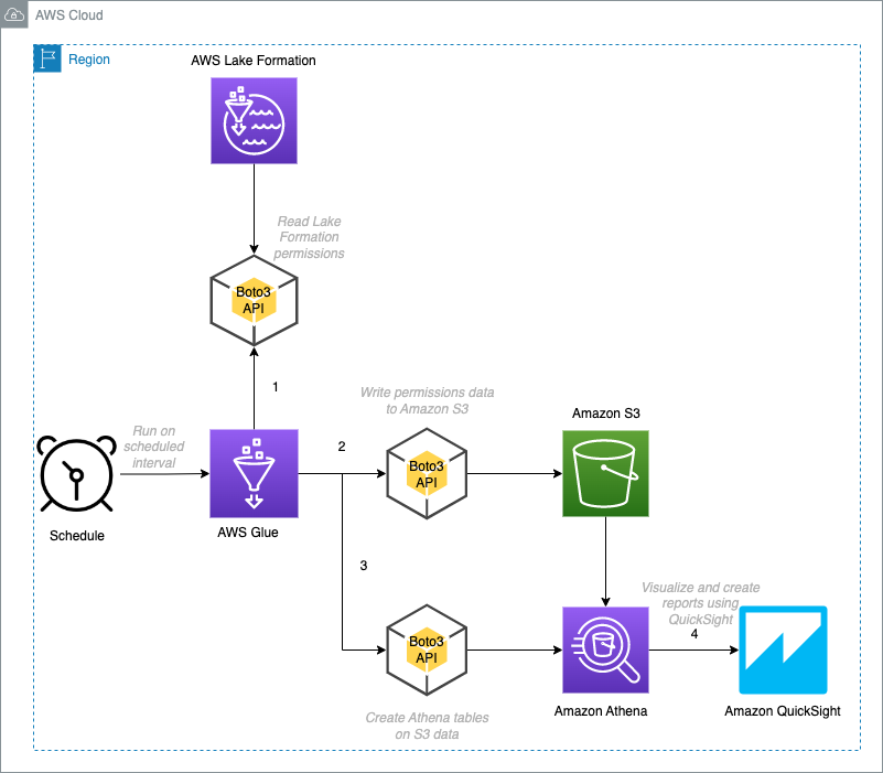
In this solution, we walk through the following tasks:
- Create an AWS Glue job to collect and store permissions data, and create external tables using Boto3.
- Verify the external tables created using Athena.
- Sign up for a QuickSight Enterprise account and enable Athena access.
- Create a dataset using an Athena data source.
- Use the datasets for analysis.
- Publish the analyses as a QuickSight dashboard.
The collected JSON data is flattened and written into an Amazon Simple Storage Service (Amazon S3) bucket as Parquet files partitioned by account ID, date, and resource type. After the data is stored in Amazon S3, external tables are created on them and filters are added for different types of resource permissions. These datasets can be imported into SPICE, an in-memory query engine that is part of QuickSight, or queried directly from QuickSight to create analyses. Later, you can publish these analyses as a dashboard and share it with other users.
Dashboards are created for the following use cases:
- Database permissions
- Table permissions
- Principal permissions
Prerequisites
You should have the following prerequisites:
- An S3 bucket to store the permissions inventory data
- An AWS Glue database for permissions inventory metadata
- An AWS Identity and Access Management (IAM) role for the AWS Glue job with access to the inventory AWS Glue database and S3 bucket and added as a data lake admin
- A QuickSight account with access to Athena
- An IAM role for QuickSight with access to the inventory AWS Glue database and S3 bucket
Set up and run the AWS Glue job
We create an AWS Glue job to collect Lake Formation permissions data for the given account and Region that is provided as job parameters, and the collected data is flattened before storage. Data is partitioned by account ID, date, and permissions type, and is stored as Parquet in an S3 bucket using Boto3. We create external tables on the data and add filters for different types of resource permissions.
To create the AWS Glue job, complete the following steps:
- Download the Python script file to local.
- On the AWS Glue console, under Data Integration and ETL in the navigation pane, choose Jobs.
- Under Create job, select Python Shell script editor.
- For Options, select Upload and edit an existing script.
- For File upload, choose Choose file.
- Choose the downloaded file (
lf-permissions-inventory.py). - Choose Create.

- After the job is created, enter a name for the job (for this post, lf-inventory-builder) and choose Save.

- Choose the Job details tab.
- For Name, enter a name for the job.
- For IAM Role¸ choose an IAM role that has access to the inventory S3 bucket and inventory schema and registered as data lake admin.
- For Type, choose Python Shell.
- For Python version, choose Python 3.9.

- You can leave other property values at their default.
- Under Advanced properties¸ configure the following job parameters and values:
catalog-id: with the value as the current AWS account ID whose permissions data are collected.databasename: with the value as the AWS Glue database where the inventory-related schema objects are created.region: with the value as the current Region where the job is configured and whose permissions data is collected.s3bucket: with the value as the S3 bucket where the collected permissions data is written.createtable: with the value yes, which enables external table creation on the data.

- Choose Save to save the job settings.

- Choose Run to start the job.
When the job is complete, the run status changes to Succeeded. You can view the log messages in Amazon CloudWatch Logs.

Permissions data is collected and stored in the S3 bucket (under lfpermissions-data) that you provided in the job parameters.

The following external tables are created on the permissions data and can be queried using Athena:
- lfpermissions – A summary of resource permissions
- lfpermissionswithgrant – A summary of grantable resource permissions
For both tables, the schema structure is the same and the lftype column indicates what type of permissions the row applies to.

Verify the tables using Athena
You can use Athena to verify the data using the following queries.
For more information, refer to Running SQL queries using Amazon Athena
- List the database permissions:
- List the table permissions:
- List the data lake permissions:
- List the grantable database permissions:
- List the grantable table permissions:
- List grantable data lake permissions:
As the next step, we create a QuickSight dashboard with three sheets, each focused on different sets of permissions (database, table, principal) to slice and dice the data.
Sign up for a QuickSight account
If you haven’t signed up for QuickSight, complete the following steps:
- Sign in to the AWS Management Console as Admin, search for QuickSight and choose Sign up for QuickSight.

- For Edition, select Enterprise.
- Choose Continue.
- For Authentication method, select Use IAM federated identities & QuickSight-managed users.
- Under QuickSight Region, choose the same Region as your inventory S3 bucket.
- Under Account info, enter a QuickSight account name and email address for notification.

- In the Quick access to AWS services section, for IAM Role, select Use QuickSight-managed role (default).
- Allow access to IAM, Athena, and Amazon S3.
- Specify the S3 bucket that contains the permissions data.
- Choose Finish to complete the signup process.

Note: If the inventory bucket and database is managed by Lake Formation, grant database and table access to the created QuickSight IAM role. For instructions, refer to Granting and revoking permissions on Data Catalog resources.
Configure your dataset in QuickSight
QuickSight is configured with an Athena data source the same Region as the S3 bucket. To set up your dataset, complete the following steps:
- On the QuickSight console, choose Datasets in the navigation pane.
- Choose New dataset.

- Choose Athena as your data source.

- Enter
LF\_DASHBOARD\_DSas the name of your data source. - Choose Create data source.
- For Catalog, leave it as AwsDataCatalog.
- For Database, choose database name provided as parameter to the Job.
- For Tables, select lfpermissions.
- Choose Select.

- Select Directly query your data and choose Visualize to take you to the analysis.

Create analyses
We create three sheets for our dashboard to view different levels of permissions.
Sheet 1: Database permission view
To view database permissions, complete the following steps:
- On the QuickSight console, choose the plus sign to create a new sheet.
- Choose Add, then choose Add title.

- Name the sheet Database Permissions.
- Repeat steps (5-7) to add the following parameters:
catalogiddatabasenamepermissiontablename
- On the Add menu, choose Add parameter.
- Enter a name for the parameter.
- Leave the other values as default and choose Create.
- Choose Insights in the navigation pane, then choose Add control.

- Add a control for each parameter:
- For each parameter, for Style¸ choose List, and for Values, select Link to a dataset field.

- Provide additional information for each parameter according to the following table.
- For each parameter, for Style¸ choose List, and for Values, select Link to a dataset field.
| Parameter | Display Name | Dataset | Field |
| catalogid | AccountID | lfpermissions | catalog\_id |
| databasename | DatabaseName | lfpermissions | databasename |
| permission | Permission | lfpermissions | permission |
- Add a control dependency and for Database, choose the options menu and choose Edit.

- Under Format control, choose Control options.
- Change the relevant values, choose AccountID, and choose Update.
- Similarly, under Permission control, choose Control options.
- Change the relevant values, choose AccountID, and choose Update.
We create two visuals for this view.
- For the first visual, choose Visualize and choose pivot table as the visual type.
- Drag and drop
catalog\_idanddatabasenameinto Rows. - Drag and drop
permissioninto Column. - Drag and drop
principalinto Values and change the aggregation to Count distinct.

- Add a filter on the
lftypefield with the following options:- Custom filter as the filter type.
- Equals as the filter condition.
- DATABASE as the value.
- Add a filter on
catalog\_idthe following options:- Custom filter as the filter type.
- Equals as the filter condition.
- Select Use parameters and choose
catalogid.
- Add a filter on
databasenamewith the following options:- Custom filter as the filter type.
- Equals as the filter condition.
- Select Use parameters and choose
databasename.
- Add a filter on
permissionwith the following options:- Custom filter as the filter type.
- Equals as the filter condition.
- Select Use parameters and choose
permission.
- Choose Actions in the navigation pane.
- Define a new action with the following parameters:
- For Activation, select Select.
- For Filter action, select All fields.
- For Target visuals, select Select visuals and Check principal.
Now we add our second visual.
- Add a second visual and choose the table visual type.
- Drag and drop
principalto Group by. - Add a filter on the
lftypefield with the following options:- Custom filter as the filter type.
- Equals as the filter condition.
- DATABASE as the value.
- Add a filter on
catalog\_idthe following options:- Custom filter as the filter type.
- Equals as the filter condition.
- Select Use parameters and choose
catalogid.
- Add a filter on
databasenamethe following options:- Custom filter as the filter type.
- Equals as the filter condition.
- Select Use parameters and choose
databasename.
- Add a filter on
permissionwith the following options:- Custom filter as the filter type.
- Equals as the filter condition.
- Select Use parameters and choose
permission.
Now the Database and Permission drop-down menus are populated based on the relevant attributes and changes dynamically.

Sheet 2: Table permission view
Now that we have created the database permissions sheet, we can add a table permissions sheet.
- Choose the plus sign to add a new sheet.
- On the QuickSight console, choose Add, then choose Add title.
- Name the sheet Table Permissions.
- Choose Insights in the navigation pane, then choose Add control.
- Add a control for each parameter:
- For each parameter, for Style¸ choose List, and for Values, select Link to a dataset field.
- Provide the additional information for each parameter according to the following table.
| Parameter | Display Name | Dataset | Field |
| catalogid | AccountID | lfpermissions | catalog\_id |
| databasename | DatabaseName | lfpermissions | databasename |
| permission | Permission | lfpermissions | permission |
| tablename | TableName | lfpermissions | tablename |
We create two visuals for this view.
- For the first visual, choose Visualize and choose pivot table as the visual type.
- Drag and drop
catalog\_id,databasename, andtablenameinto Rows. - Drag and drop
permissioninto Column. - Drag and drop
principalinto Values and change the aggregation to Count distinct. - Add a filter on the
lftypefield with the following options:- Custom filter as the filter type.
- Equals as the filter condition.
- TABLE as the value.
- Add a filter on
catalog\_idthe following options:- Custom filter as the filter type.
- Equals as the filter condition.
- Select Use parameters and choose
catalogid.
- Add a filter on the
databasenamewith the following options:- Custom filter as the filter type.
- Equals as the filter condition.
- Select Use parameters and choose
databasename.
- Add a filter on
tablenamewith the following options:- Custom filter as the filter type.
- Equals as the filter condition.
- Select Use parameters and choose
tablename.
- Add a filter on
permissionwith the following options:- Custom filter as the filter type.
- Equals as the filter condition.
- Select Use parameters and choose
permission.
- Choose Actions in the navigation pane.
- Define a new action with the following parameters:
- For Activation, select Select.
- For Filter action, select All fields.
- For Target visuals, select Select visuals and Check principal.
Now we add our second visual.
- Add a second visual and choose the table visual type.
- Drag and drop
principalto Group by. - Add a filter on the
lftypefield with the following options:- Custom filter as the filter type.
- Equals as the filter condition.
- TABLE as the value.
- Add a filter on
catalog\_idthe following options:- Custom filter as the filter type.
- Equals as the filter condition.
- Select Use parameters and choose
catalogid.
- Add a filter on the
databasenamewith the following options:- Custom filter as the filter type.
- Equals as the filter condition.
- Select Use parameters and choose
databasename.
- Add a filter on
tablenamewith the following options:- Custom filter as the filter type.
- Equals as the filter condition.
- Select Use parameters and choose
tablename.
- Add a filter on
permissionwith the following options:- Custom filter as the filter type.
- Equals as the filter condition.
- Select Use parameters and choose
permission.
Now the Databasename, Tablename, and Permission drop-down menus are populated based on the relevant attributes.

Sheet 3: Principal permission view
Now we add a third sheet for principal permissions.
- Choose the plus sign to add a new sheet.
- On the QuickSight console, choose Add, then choose Add title.
- Name the sheet Principal Permissions.
- Choose Insights in the navigation pane, then choose Add control.
- Add a control for the
catalogidparameter:- For Style¸ choose List, and for Values, select Link to a dataset field.
- Provide the additional information for the parameter according to the following table.
| Parameter | Display Name | Dataset | Field |
| catalogid | AccountID | lfpermissions | catalog\_id |
We create four visuals for this view.
- For the first visual, choose Visualize and choose pivot table as the visual type.
- Drag and drop
catalog\_idandprincipalinto Rows. - Drag and drop
permissioninto Column. - Drag and drop
databasenameinto Values and change the aggregation to Count distinct. - Add a filter on the
lftypefield with the following options:- Custom filter as the filter type.
- Equals as the filter condition.
- DATABASE as the value.
- Add a filter on the
catalog\_idfield with the following options:- Custom filter as the filter type.
- Equals as the filter condition.
- Select Use parameters and choose
catalogid.
- Choose Actions in the navigation pane.
- Define a new action with the following parameters:
- For Activation, select Select.
- For Filter action, select All fields.
- For Target visuals, select Select visuals and Check Databasename.
- For the second visual, choose Visualize and choose table as the visual type.
- Drag and drop
databasenameinto Group by. - Add a filter on the
lftypefield with the following options:- Custom filter as the filter type.
- Equals as the filter condition.
- DATABASE as the value.
- Add a filter on the
catalog\_idfield with the following options:- Custom filter as the filter type.
- Equals as the filter condition.
- Select Use parameters and choose
catalogid.
- For the third visual, choose Visualize and choose pivot table as the visual type.
- Drag and drop
catalog\_idandprincipalinto Rows. - Drag and drop
permissioninto Column. - Drag and drop
tablenameinto Values and change the aggregation to Count distinct. - Add a filter on the
lftypefield with the following options:- Custom filter as the filter type.
- Equals as the filter condition.
- TABLE as the value.
- Add a filter on the
catalog\_idfield with the following options:- Custom filter as the filter type.
- Equals as the filter condition.
- Select Use parameters and choose
catalogid.
- Choose Actions in the navigation pane.
- Define a new action with the following parameters:
- For Activation, select Select.
- For Filter action, select All fields.
- For Target visuals, select Select visuals and Check Tablename.
- For the final visual, choose Visualize and choose table as the visual type.
- Drag and drop
tablenameinto Group by. - Add a filter on the
lftypefield with the following options:- Custom filter as the filter type.
- Equals as the filter condition.
- TABLE as the value.
- Add a filter on the
catalog\_idfield with the following options:- Custom filter as the filter type.
- Equals as the filter condition.
- Select Use parameters and choose
catalogid.
The following screenshot shows our sheet.

Create a dashboard
Now that the analysis is ready, you can publish it as a dashboard and share it with other users. For instructions, refer to the tutorial Create an Amazon QuickSight dashboard.
Clean up
To clean up the resources created in this post, complete the following steps:
- Delete the AWS Glue job
lf-inventory-builder. - Delete the data stored under the bucket provided as the value of the
s3bucketjob parameter. - Drop the external tables created under the schema provided as the value of the
databasenamejob parameter. - If you signed up for QuickSight to follow along with this post, you can delete the account.
- For an existing QuickSight account, delete the following resources:
lfpermissionsdatasetlfpermissionsanalysislfpermissionsdashboard
Conclusion
In this post, we provided a design and implementation steps for a solution to collect Lake Formation permissions in a given Region of an account and consolidate them for analysis. We also walked through the steps to create a dashboard using Amazon QuickSight. You can utilize other QuickSight visuals to create more sophisticated dashboards based on your requirements.
You can also expand this solution to consolidate permissions for a multi-account setup. You can use a shared bucket across organizations and accounts and configure an AWS Glue job in each account or organization to write their permission data. With this solution, you can maintain a unified dashboard view of all the Lake Formation permissions within your organization, thereby providing a central audit mechanism to comply with business requirements.
Thanks for reading this post! If you have any comments or questions, please don’t hesitate to leave them in the comments section.
About the Author
Srividya Parthasarathy is a Senior Big Data Architect on the AWS Lake Formation team. She enjoys building analytics and data mesh solutions on AWS and sharing them with the community.
Amazon Redshift is a fully managed, petabyte scale cloud data warehouse that enables you to analyze large datasets using standard SQL. Data warehouse workloads are increasingly being used with business-critical analytics applications that require the highest levels of availability and resiliency. Amazon Redshift is a cloud-based data warehouse that already supports many recovery capabilities to address unforeseen outages and minimize downtime. Amazon Redshift RA3 instance types store their data in Redshift Managed Storage (RMS), which is backed by Amazon Simple Storage Service (Amazon S3), which is highly available and durable by default. Amazon Redshift also supports automatic backups that can be used to recover a data warehouse, automatic remediation of failures, and the ability to relocate a cluster to another Availability Zone without changes to applications. Although many customers benefit from these features, enterprise data warehouse customers require a low RTO and higher availability to support their business continuity with minimal impact to applications.
Amazon Redshift now supports Multi-AZ deployments (Preview) for provisioned RA3 clusters. Multi-AZ deployments support running your data warehouse in multiple Availability Zones simultaneously and can continue operating in unforeseen failure scenarios. A Multi-AZ deployment is intended for customers with business-critical analytics applications that require the highest levels of availability and resiliency.
A Redshift Multi-AZ deployment leverages compute resources in multiple AZs to scale data warehouse workload processing. In situations where there is a high level or concurrency Redshift will automatically leverage the resources in both AZs to scale the workload for both read and write requests using active-active processing.
In this post, we show how to configure an Amazon Redshift Multi-AZ deployment in multiple Availability Zones.
Overview of solution
We provide a walkthrough of how to perform a Multi-AZ deployment for an Amazon Redshift cluster using the AWS Management Console. We also provide a walkthrough on how to test fault tolerance of an Amazon Redshift Multi-AZ data warehouse and monitor queries in your Multi-AZ deployment.
Single-AZ vs. Multi-AZ deployment
Amazon Redshift requires a cluster subnet group to create a cluster in your VPC. The cluster subnet group includes information about the VPC ID and a list of subnets in your VPC. When you launch a cluster, Amazon Redshift either creates a default cluster subnet group automatically or you choose a cluster subnet group of your choice so that Amazon Redshift can provision your cluster in one of the subnets in the VPC. You can configure your cluster subnet group to add subnets from different Availability Zones that you want Amazon Redshift to use for cluster deployment.
All Amazon Redshift clusters today are created and situated in a particular Availability Zone within an AWS Region and thus called Single-AZ deployments. For a Single-AZ deployment, Amazon Redshift selects the subnet from one of the Availability Zones within a Region and deploys the cluster there. You can choose an Availability Zone for deployment, and Amazon Redshift will deploy your cluster in the chosen Availability Zone based on the subnets provided.
On the other hand, a multi-AZ deployment is provisioned in multiple Availability Zones simultaneously. For a Multi-AZ deployment, Amazon Redshift automatically selects two subnets from two different Availability Zones and deploys an equal number of compute nodes in each Availability Zone. All these compute nodes are utilized via a single endpoint as compute nodes from both Availability Zones are used for workload processing.
As shown in the following diagrams, Amazon Redshift deploys a cluster in a single Availability Zone for Single-AZ deployment, and multiple Availability Zones for Multi-AZ deployment.
 |  |
Auto recovery of multi-AZ deployment
In the unlikely event of an Availability Zone failure, Amazon Redshift Multi-AZ deployments continue to serve your workloads by automatically using resources in the other Availability Zone. You are not required to make any application changes to maintain business continuity during unforeseen outages since a multi-AZ deployment is accessed as a single data warehouse with one endpoint. Amazon Redshift Multi-AZ deployments are designed to ensure there is no data loss, and you can query all data committed up until the point of failure.
As shown in the below diagram, if there is an unlikely event that causes compute nodes in AZ1 to fail, then a multi-AZ deployment automatically recovers to use compute resources in AZ2. Amazon Redshift will also automatically provision identical compute nodes in another availability zone (AZ3) to continue operating simultaneously in two Availability zones (AZ2 and AZ3).
 |  |
Amazon Redshift Multi-AZ deployment is not only used for protection against the possibility of Availability Zone failures, but it can also maximize your data warehouse performance by automatically distributing workload processing across multiple Availability Zones. A Multi-AZ deployment will always process an individual query using compute resources only from one Availability Zone, but it can automatically distribute processing of multiple simultaneous queries to both Availability Zones to increase overall performance for high concurrency workloads.
It’s a good practice to set up automatic retries in your extract, transform, and load (ETL) processes and dashboards so that they can be reissued and served by the cluster in the secondary Availability Zone when an unlikely failure happens in the primary Availability Zone. If a connection is dropped, it can then be retried or reestablished immediately. In addition, queries and loads that were running in the failed Availability Zone will be aborted. New queries issued at or after a failure occurs may experience run delays while the multi-AZ data warehouse is being are recovered to a two AZ setup.
Create a new Multi-AZ deployment from the console
You can easily create a new multi-AZ deployments through Amazon Redshift console. Amazon Redshift will deploy the same number of nodes in each of the two Availability Zones for a Multi-AZ deployment. All nodes of a multi-AZ deployment can perform read and write workload processing during normal operation. A Multi-AZ deployment will support only provisioned RA3 clusters.
Follow these steps to create an Amazon Redshift provisioned cluster in multiple Availability Zones:
- On the Amazon Redshift console, in the navigation pane, choose Clusters.
- A banner displays on the Clusters list page that introduces preview mode. Choose the button Create preview cluster to open the create cluster page.
- For Preview track, choose preview\_2022.
- We recommend entering a name for the cluster that indicates that it is on a preview track. Choose options for your cluster, including options labeled as -preview, for the features you want to test.
For general information about creating clusters, see Creating a cluster.
- Choose one of the RA3 node types on the Node type drop-down menu. The Multi-AZ deployment option only becomes available when you choose an RA3 node type.
- For Multi-AZ deployment, select Yes.
- For Number of nodes per AZ, enter the number of nodes that you need for your cluster.

- Under the Database configurations, choose Admin user name and Admin user password.
- Turn Use defaults on next to Additional configurations to modify the default settings.
- Under Network and security, specify the following:
- For Virtual private cloud (VPC), choose the VPC you want to deploy the cluster in.
- For VPC security groups, either leave as default or add the security groups of your choice.
- For Cluster subnet group, either leave as default or add a cluster subnet group of your choice. For a Multi-AZ deployment, a cluster subnet group must include one subnet each from at least three or more different Availability Zones.
For general information about managing cluster subnet groups, see Cluster subnet groups

- Under Database configuration, for Database port, you either use the default value 5439 or choose a value from the range of 5431–5455 and 8191–8215.
- Under Database configuration, in the Database encryption section, to use a custom AWS Key Management Service (AWS KMS) key other than the default KMS key, choose Customize encryption settings. This option is deselected by default.
- Under Choose an AWS KMS key, you can either choose an existing KMS key, or choose Create an AWS KMS key to create a new KMS key.
For more information to create key using KMS, refer to Creating keys.

- Choose Create cluster.
When the cluster creation succeeds, you can view the details on the cluster details page.
Under General information, you can see Multi-AZ as Yes.

On the Properties tab, under Network and security settings, you can find the details on the primary and secondary Availability Zone.

Convert a Single-AZ deployment to Multi-AZ deployment
To convert an existing Single-AZ deployment to a Multi-AZ deployment, you can restore from a snapshot to configure it into a Multi-AZ data warehouse. When migrating to a Multi-AZ deployment from an existing Single-AZ deployment, maintaining performance of a single query may require the same number of nodes used in the current Single-AZ deployment to be provisioned in both Availability Zones, resulting in doubling the amount of cluster nodes needed when migrating to Multi-AZ to ensure that single query performance is maintained.
Complete the following steps to create a Multi-AZ deployment restored from a snapshot:
- On the Amazon Redshift console, in the navigation pane under Clusters, choose Snapshots.
- Select the snapshot to use.
- The snapshot needs to be encrypted in order to restore to a Multi-AZ deployment.
- On the Restore snapshot menu, choose Restore to provisioned cluster.

- Choose the Preview mode.
- For Preview track, choose preview\_2022
- We recommend entering a name for the cluster that indicates that it is on a preview track. Choose options for your cluster, including options labeled as -preview, for the features you want to test.
For general information about creating clusters, see Creating a cluster.
- Make sure that you choose one of the RA3 node types on the Node type drop-down menu. The Multi-AZ deployment option only becomes available when you chose an RA3 node type.
- For Multi-AZ deployment, select Yes.
- For Number of nodes per AZ, enter the number of nodes that you need for your cluster.

- Scroll down to Additional configurations, expand Network and security, make sure that you either accept the default for Cluster subnet group or choose another one of your choice. For a Multi-AZ deployment, a cluster subnet group must include one subnet each from at least three or more different Availability Zones.
- Under Additional configurations, expand Database configurations.
- Under Database encryption, to use a custom KMS key other than the default KMS key, choose Customize encryption settings. This option is deselected by default.
- Under Choose an AWS KMS key, you can either choose a KMS key or enter an ARN. Or, you can choose Create an AWS Key Management Service key to create a key.

- Choose Restore cluster from snapshot.
When the cluster restoration succeeds, you can view the details on the cluster details page.
Test fault tolerance of your multi-AZ data warehouse
You can test the fault tolerance of your Amazon Redshift Multi-AZ deployment by injecting a failure that causes compute nodes in one Availability Zone to become unavailable. Amazon Redshift detects this event and triggers an automatic recovery. When the cluster successfully recovers, Multi-AZ deployment becomes available. Your Multi-AZ deployment also automatically provisions new compute nodes in another Availability Zone as soon as it is available.
Let’s test the fault tolerance of the Amazon Redshift Multi-AZ deployment.
- On the Amazon Redshift console, choose Clusters in the navigation pane.
- Navigate to the cluster detail page
- On the Actions menu, choose Inject Failure (Public Preview).

- When prompted, choose Confirm.

After the cluster is back to Available status, you can observe that the primary and secondary Availability Zones have changed.
The following screenshot shows the status before injecting failure.

The following screenshot shows the status after injecting failure.

Monitor queries for Multi-AZ deployments
A Multi-AZ deployment uses compute resources that are deployed in both Availability Zones and can continue operating in the event that the resources in a given Availability Zone are not available. All the compute resources are used at all times, which allows full operation across two Availability Zones in both read and write operations.
You can query SYS\_ views in the pg\_catalog schema to monitor Multi-AZ query runs. The SYS\_ views cover query run activities and stats from primary and secondary clusters.
The following are the system tables in the SYS\_ view list:
- SYS\_QUERY\_HISTORY
- SYS\_QUERY\_DETAIL
- SYS\_CONNECTION\_LOG
- SYS\_DATASHARE\_CHANGE\_LOG
- SYS\_DATASHARE\_USAGE\_CONSUMER
- SYS\_DATASHARE\_USAGE\_PRODUCER
- SYS\_EXTERNAL\_QUERY\_DETAIL
- SYS\_LOAD\_HISTORY
- SYS\_LOAD\_ERROR\_DETAIL
- SYS\_UNLOAD\_HISTORY
Follow these steps to monitor the query run on Multi-AZ deployment from the Amazon Redshift Console:
- On the Amazon Redshift console, connect to the database in your Multi-AZ deployment and run queries through the query editor.
- Run any sample query on the Multi-AZ Redshift deployment.
- For a Multi-AZ deployment, you can identify a query and the Availability Zone where it is being run (running on the primary cluster or secondary availability zone) by using the
compute\_typecolumn in theSYS\_QUERY\_HISTORYtable. The valid values for thecompute typecolumn are as follows:- primary – When run on primary availability zone in the Multi-AZ deployment.
- secondary – When run on secondary availability zone in the Multi-AZ deployment.
The following is a sample query using the compute\_type column to monitor a query:
You can also access the query history from the console to analyze your query diagnostics.
- On the Query monitoring tab, choose Connect to database.

- For Authentication, choose Temporary credentials
- For Database name, enter the database name (for example,
dev). - For Database user, enter the database user name (for example,
awsuser). - Choose Connect.

After you’re connected, under Query Monitoring, on the Query history tab, you can view all the queries and loads, as shown in the following screenshot.

Under Metric filters, you can use the various filters in the Additional filtering options section to view query history based on Time interval, Users, Databases, or SQL commands.

There are a few limitations when working with Amazon Redshift Multi-AZ in preview mode, refer here for the limitations.
Customer feedback
 | Janssen Pharmaceuticals, a subsidiary of Johnson & Johnson, researches and manufactures medicines with a focus on the changing needs of patients and the healthcare industry.
– Shyam Mohapatra, Director of Information Technology – Janssen Pharmaceutical Companies of Johnson & Johnson |
Conclusion
This post demonstrated how to configure an Amazon Redshift Multi-AZ deployment in multiple Availability Zones and test the fault tolerance of your workloads during an unlikely failure of an Availability Zone. Amazon Redshift Multi-AZ deployment also helps improve overall performance of your data warehouse because compute nodes in both Availability Zones are used for read and write operations. Amazon Redshift Multi-AZ data warehouse helps meets the demands of customers with business critical analytics applications that require the highest levels of availability and resiliency.
For more details, refer Configuring Multi-AZ deployment.
About the Authors
 Ranjan Burman is an Analytics Specialist Solutions Architect at AWS. He specializes in Amazon Redshift and helps customers build scalable analytical solutions. He has more than 16 years of experience in different database and data warehousing technologies. He is passionate about automating and solving customer problems with cloud solutions.
 Jeff Sosa leads the Redshift product management team responsible for the core redshift compute and storage platform, availability, backup/recovery and disaster recovery areas. Jeff has been at AWS for over 3 years and has focused on high-scale distributed systems processing and storage throughout his 20 year career in product management.
 Saurav Das is part of the Amazon Redshift Product Management team. He has more than 16 years of experience in working with relational databases technologies and data protection. He has a deep interest in solving customer challenges centered around high availability and disaster recovery.
Anusha Challa is a Senior Analytics Specialist Solutions Architect focused on Amazon Redshift. She has helped many customers build large-scale data warehouse solutions in the cloud and on premises. She is passionate about data analytics and data science.
 Nita Shah is an Analytics Specialist Solutions Architect at AWS based out of New York. She has been building data warehouse solutions for over 20 years and specializes in Amazon Redshift. She is focused on helping customers design and build enterprise-scale well-architected analytics and decision support platforms.
 Suresh Patnam is a Principal BDM – GTM AI/ML Leader at AWS. He works with customers to build IT strategy, making digital transformation through the cloud more accessible by using data and AI/ML. In his spare time, Suresh enjoys playing tennis and spending time with his family.
Amazon DynamoDB is ideal for applications that need a flexible NoSQL database with low read and write latencies and the ability to scale storage and throughput up or down as needed without code changes or downtime. You can use DynamoDB for use cases including mobile apps, gaming, digital ad serving, live voting, audience interaction for live events, sensor networks, log ingestion, access control for web-based content, metadata storage for Amazon S3 objects, e-commerce shopping carts, and web session management.
What if you have the need to allow other AWS accounts to query your DynamoDB table? What if other accounts need to join data on your DynamoDB table with their data stored in data sources like Amazon CloudWatch, Amazon DocumentDB, Amazon Redshift, Amazon OpenSearch, MySQL, PostgreSQL connected with Athena data source connectors, and Amazon S3?
Amazon Athena cross-account federated query enables you to run SQL queries across data stored in relational, non-relational, object, and custom data sources where data source and its connector are in different AWS accounts from the user querying the data. There are no new charges for querying connectors in another account, but Athena’s standard rates for data scanned, Lambda usage, and other services apply.
This post will demonstrate Athena in an AWS account accessing a DynamoDB table of another AWS account by using the Athena cross-account federated query. It also explains deploying Amazon Athena DynamoDB connector using AWS Serverless Application Repository and setting up Athena cross-account federation between two accounts for the Demo.
Walkthrough
The solution has the following steps to demonstrate Athena cross-account federated query:
- Set up Athena federation – To deploy a Lambda function for the data source connector and connect it to a data source.
- Set up Athena cross-account federation – To set up IAM permissions for Athena cross-account federation.
- Test Athena cross-account federated query – To show a demo of how an AWS account can share its DynamoDB table as an Athena data source with another AWS account.
Prerequisites
For this walkthrough, you should have the following prerequisites:
- Two AWS Accounts
- AWS resources: Amazon Simple Storage Service (Amazon S3), Amazon Athena, Amazon DynamoDB, AWS Lambda
Data source connectors
A data source connector is a piece of code that can translate between your target data source and Athena. Athena uses data source connectors that run on AWS Lambda to run federated queries. You can think of a connector as an extension of Athena’s query engine.
Connectors use Apache Arrow as the format for returning data requested in a query, which enables connectors to be implemented in languages such as C, C++, Java, Python, and Rust.
Athena uses data source connectors that run on AWS Lambda to run federated queries. Since connectors are processed in Lambda, they can be used to access data from any data source on the cloud or on premises that is accessible from Lambda
To use a connector in your Athena queries, deploy it to your account using one of the following ways:
- AWS Serverless Application Repository
- Athena and Lambda consoles
This blog uses the AWS Serverless Application Repository to deploy the Amazon Athena DynamoDB connector.
After you deploy data source connectors, the connector is associated with a catalog that you can specify in SQL queries. You can combine SQL statements from multiple catalogs and span multiple data sources with a single query. When a query is submitted against a data source, Athena invokes the corresponding connector to identify parts of the tables that need to be read, manages parallelism, and pushes down filter predicates. Based on the user submitting the query, connectors can provide or restrict access to specific data elements.
Architecture
- AWS Account-A has a DynamoDB table called
Music. - Account-A has an Athena data source connector to federate into DynamoDB.
- AWS Account-B has Analysts who need to query the DynamoDB table.
- Account-A is sharing the Athena data source with Account-B by using Athena cross-account federated query.
The following figure shows Amazon Athena cross-account federation for Account-B to access DynamoDB in Account-A.

To demonstrate the Athena cross-account federation, create a sample DynamoDB table called music in Account-A. Follow the instructions at Getting started with DynamoDB to create the table Music and load thesample data.
Set up Athena federation
Preparing to create federated queries is a two-part process: deploying a Lambda function for the data source connector and connecting the Lambda function to a data source. For more details, see Enabling cross-account federated queries.
Deploy AthenaDynamoDBConnector using AWS Serverless Application Repository
- Sign in as an administrator to AWS Account-A.
- Open the Serverless Application Repository.
- In the navigation pane, choose Available applications.
- Select the option Show apps that create custom IAM roles or resource policies.
- In the search box, type the name of the connector
AthenaDynamoDBConnector.


- Choosing a connector opens the Lambda function’s Application details page in the AWS Lambda console.
- On the right side of the details page, for Application settings, fill in the required information.
- Application name – Name of AWS CloudFormation Stack to deploy the connector:
AthenaDynamoDBConnector. - AthenaCatalogName – It is the catalog name to create in Athena. It is also the name of the Lambda function. Give it in lowercase:
acct1dynamodb. - SpillBucket – Specify an existing S3 bucket (
spill-bucket) in your account to receive data from any large response payloads that exceed Lambda function response size limits.

- Application name – Name of AWS CloudFormation Stack to deploy the connector:
- Select I acknowledge that this app creates custom IAM roles and resource policies. For more information, choose the Info link.
- At the bottom right of the Application settings section, choose Deploy.
- Serverless Application Repository will create an AWS CloudFormation stack to deploy the connector.
- When the deployment is complete, you will see the Lambda function in the Resources section of the AWS CloudFormation stack. Note down the Lambda function name.


Connect Athena to the data source
- Go to Athena console in Account-A.
- Choose Data sources. Click Create Data source.

- In Choose data source, search for Amazon DynamoDB and select it.

- In Data source details, give a Data source name
acct1dynamodb

- For Lambda function in the Connection details section, choose the name of the function
acct1dynamodbfrom the dropdown.

- On the Review and create page, review the data source details, and then choose Create data source.


- You will see the data source
acctdynamodbin the Data sources.

- Go to Query editor. Choose the Data Source
acct1dynamodbfrom the dropdown.

- You will see all the tables in the shared data source.

- Run the following SQL in Athena Query editor
- Verify Athena federation works.

Set up Athena cross-account federation
In Account-A: Set up IAM permissions for cross-account
- Sign in as an administrator to Account-A.
- On the S3 spill bucket (of the Lambda function), grant GetObject and ListBucket permissions to the IAM user analyst of Account-B.
Note: Replace Account-B-id with your actual AWS cross-account id to which you want to share the DynamoDB table. Replace spill-bucket with your actual S3 bucket in Account-A.
- Grant InvokeFunction on Lambda function
acct1dynamodbto IAM user analyst of Account-B.
Note: Replace Account-A-id with your actual AWS account id where you have the DynamoDB table. Replace Account-B-id with your actual AWS cross-account id to which you want to share the DynamoDB table.
- Go to the Lambda function
acct1dynamodb. Choose Configuration and Permissions.

- Go to Resource-based policy and Add permissions.


When you save the above permissions, you can see them under Policy statements in Resource-based policy of the Lambda function.

In Account-B: Set up IAM permissions for cross-account
- Sign in as an administrator to AWS Account-B.
- Create IAM role called
AthenaCrossAccountFederated-Account-A-idfor Account-A to assume. Add the following inline policy to the role.
Note: Replace Account-B-id with your actual AWS cross-account id to which you want to share the DynamoDB table.
- Grant permission to the IAM user analyst to invoke the Lambda function
acct1dymanodbof Account-A

Note: Replace Account-A-id with your actual AWS account id where you have the DynamoDB table.
Share the Athena Data source with Account-B
After the permissions are in place, you share a data connector in your account (Account-A) with another account (Account-B). Account-A retains full control and ownership of the connector. When Account-A makes configuration changes to the connector, the updated configuration applies to the shared connector in Account-B.
- Sign in as an administrator to Account-A.
- On Athena, go to Data sources, choose data source
acct1dynamodbyou want to share. Go to the Share option in the top right corner.

- For Account ID, enter the Account-B-id to share your data source with Account-B and click Share.


Test Athena cross-account federated query: Access the shared data source from Account-B
- Sign in as IAM user analyst to Account-B.
- In Athena, go to Data sources. You will see the data source
acct1dynamodb.

- Go to Query editor. Choose the Data Source
acct1dynamodbfrom the dropdown.
- You will see all the tables in the shared data source.
- Run the following SQL in Athena Query editor
- Athena cross-account federated has worked! This validates that user analyst in Account-B can see the data of the DynamoDB table of Account-A.
Clean up
To avoid incurring future charges, delete the following resources that were provisioned for this demo:
- S3 spill bucket used in AWS Lambda
- Lambda function used for the data source connector
- Sample DynamoDB table
Conclusion
In this post, we saw how you can access a cross-account DynamoDB table using Athena Federated Query to query the data in place. You can execute a single SQL query to join this data across data sources like Amazon CloudWatch, Amazon DocumentDB, Amazon Redshift, Amazon OpenSearch, MySQL, PostgreSQL, Oracle, SQL Server, HBase, Redis, BigQuery, Snowflake, Teradata with Athena data source connectors and Amazon S3.
About the author
 Satya Adimula is a Senior Data Architect at AWS based in Boston. With extensive experience in data and analytics, Satya helps organizations derive their business insights from the data at scale.
This post was co-written with Vijay Chitoor, Co-Founder & CEO, and Mehul Shah, Co-Founder and CTO from the Blueshift team, as the lead authors.
Blueshift is a San Francisco-based startup that helps marketers deliver exceptional customer experiences on every channel, delivering relevant personalized marketing. Blueshift’s SmartHub Customer Data Platform (CDP) empowers marketing teams to activate their first-party customer data to drive 1:1 personalization on owned (email, mobile) and paid (Google, Facebook, and so on) website and customer (CX) channels.
In this post, Blueshift’s founding team discuss how they used Amazon Redshift Data API to integrate data from their customer’s Amazon Redshift data warehouse with their CDP environment to help marketers activate their enterprise data and drive growth for their businesses.
Business need
In today’s omnichannel world, marketing teams at modern enterprises are being tasked with engaging customers on multiple channels. To successfully deliver intelligent customer engagement, marketers need to operate with a 360 degree view of their customers that takes into account various types of data, including customer behavior, demographics, consent and preferences, transactions, data from human assisted and digital interactions, and more. However, unifying this data and making it actionable for marketers is often a herculean task. Now, for the first time, with the integration of Blueshift with Amazon Redshift, companies can use more data than ever for intelligent cross-channel engagement.
Amazon Redshift is a fast, fully managed cloud data warehouse. Tens of thousands of customers use Amazon Redshift as their analytics infrastructure. Users such as data analysts, database developers, and data scientists use SQL to analyze their data in Amazon Redshift data warehouses. Amazon Redshift provides a web-based query editor in addition to supporting connectivity via ODBC/JDBC or the Redshift Data API.
Blueshift aims at empowering business users to unlock data in such data warehouses and activate audiences with personalized journeys for segmentation, 1:1 messaging, website, mobile, and paid media use cases. Moreover, Blueshift can help combine this data in Amazon Redshift data warehouses with real-time website and mobile data for real-time profiles and activation, enabling this data to be used by marketers in these businesses.
Although the data in Amazon Redshift is incredibly powerful, marketers are unable to use it in it’s original form for customer engagement for a variety of reasons. Firstly, querying the data requires knowledge of query languages like SQL, which marketers aren’t necessarily adept at. Furthermore, marketers need to combine the data in the warehouse with additional sources of data that are critical for customer engagement, including real-time events (for example, a website page viewed by a customer), as well as channel-level permissions and identity.
With the new integration, Blueshift customers can ingest multidimensional data tables from Amazon Redshift (for example, a customer table, transactions table, and product catalog table) into Blueshift to build a single customer view that is accessible by marketers. The bi-directional integration also ensures that predictive data attributes computed in Blueshift, as well as campaign engagement data from Blueshift, are written back into Amazon Redshift tables, enabling technology and analytics teams to have a comprehensive view of the data.
In this post, we describe how Blueshift integrates with Amazon Redshift. We highlight the bi-directional integration with data flowing from a customer’s Amazon Redshift data warehouse to Blueshift’s CDP environment and vice versa. These mechanisms are facilitated through the use of the Redshift Data API.
Solution overview
The integration between the two environments is achieved through a connector. We discuss the connector’s core components in this section. Blueshift uses a hybrid approach using Redshift S3 UNLOAD, Redshift S3 COPY, and the Redshift Data API to simplify the integration between Blueshift and Amazon Redshift, thereby facilitating the data needs to empower marketing teams. The following flow diagram shows the overview of the solution.
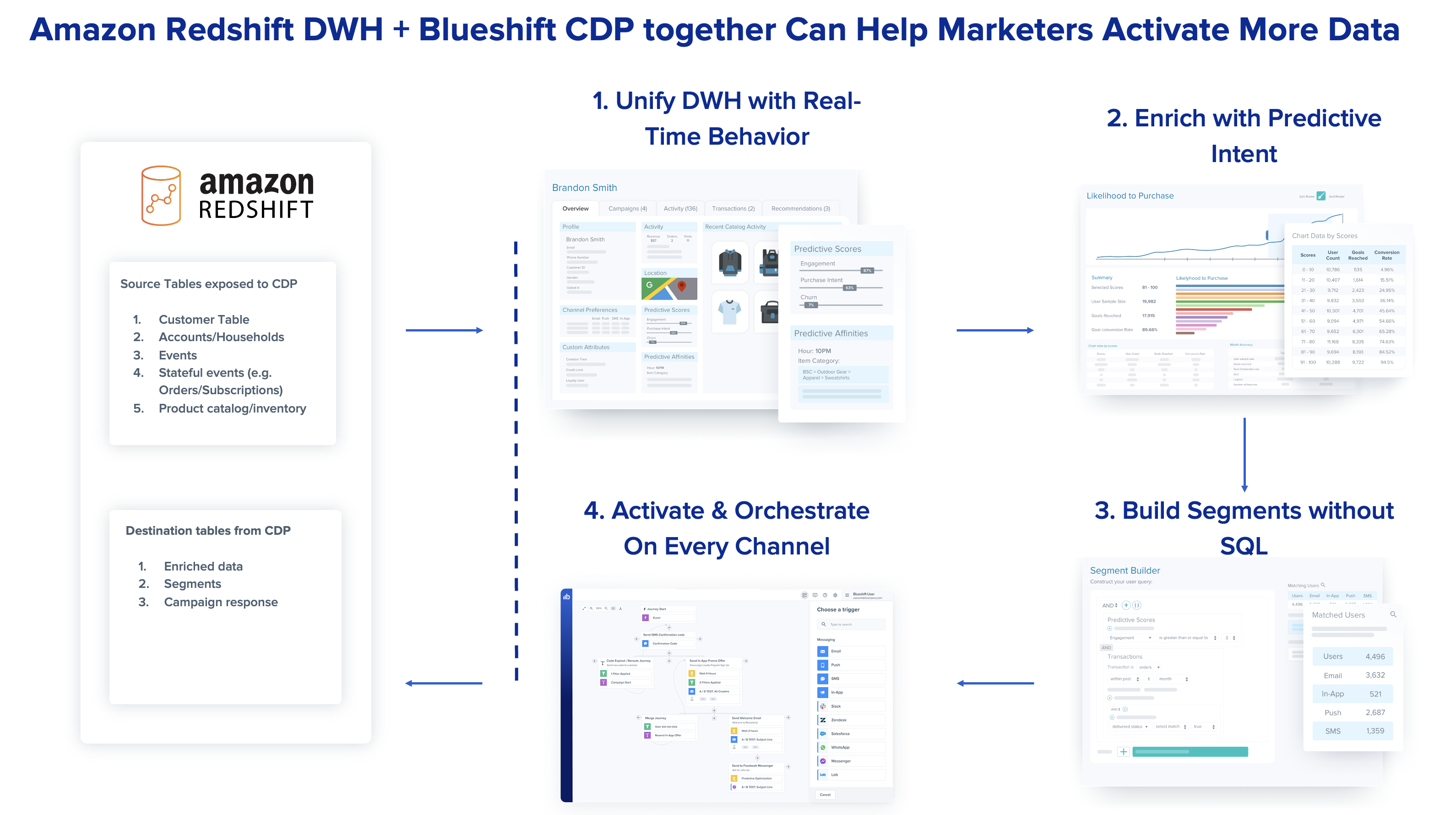
Blueshift uses container technology to ingest and process data. The data ingestion and egress containers are scaled up and down depending on the amount of data being processed. One of the key design tenets was to simplify the design by not having to manage connections or active connection pools. The Redshift Data API supports a HTTP-based SQL interface without the need for actively managing connections. As depicted in the process flow, the Redshift Data API lets you access data from Amazon Redshift with various types of traditional, cloud-native, containerized, serverless web service-based applications and event-driven applications. The Blueshift application includes a mix of programming languages, including Ruby (for the customer-facing dashboard), Go (for container workloads), and Python (for data science workloads). The Redshift Data API supports bindings in Python, Go, Java, Node.js, PHP, Ruby, and C++, which makes it simple for developer teams to integrate quickly.
With the Redshift Data API integration in place in Blueshift’s application, IT users from Blueshift customers can set up and validate the data connection, and subsequently Blueshift’s business users (marketers) can seamlessly extract value from data by developing insights and putting those insights into action for the customer data housed in AWS Redshift seamlessly. Therefore, the process developed by Blueshift using the Redshift Data API significantly lowers the barrier for entry for new users without needing data warehousing experience or ongoing IT dependencies for the business user.
The solution architecture depicted in the following figure shows how the various components of the CDP environment and Amazon Redshift integrate to provide the the end-to-end solution.
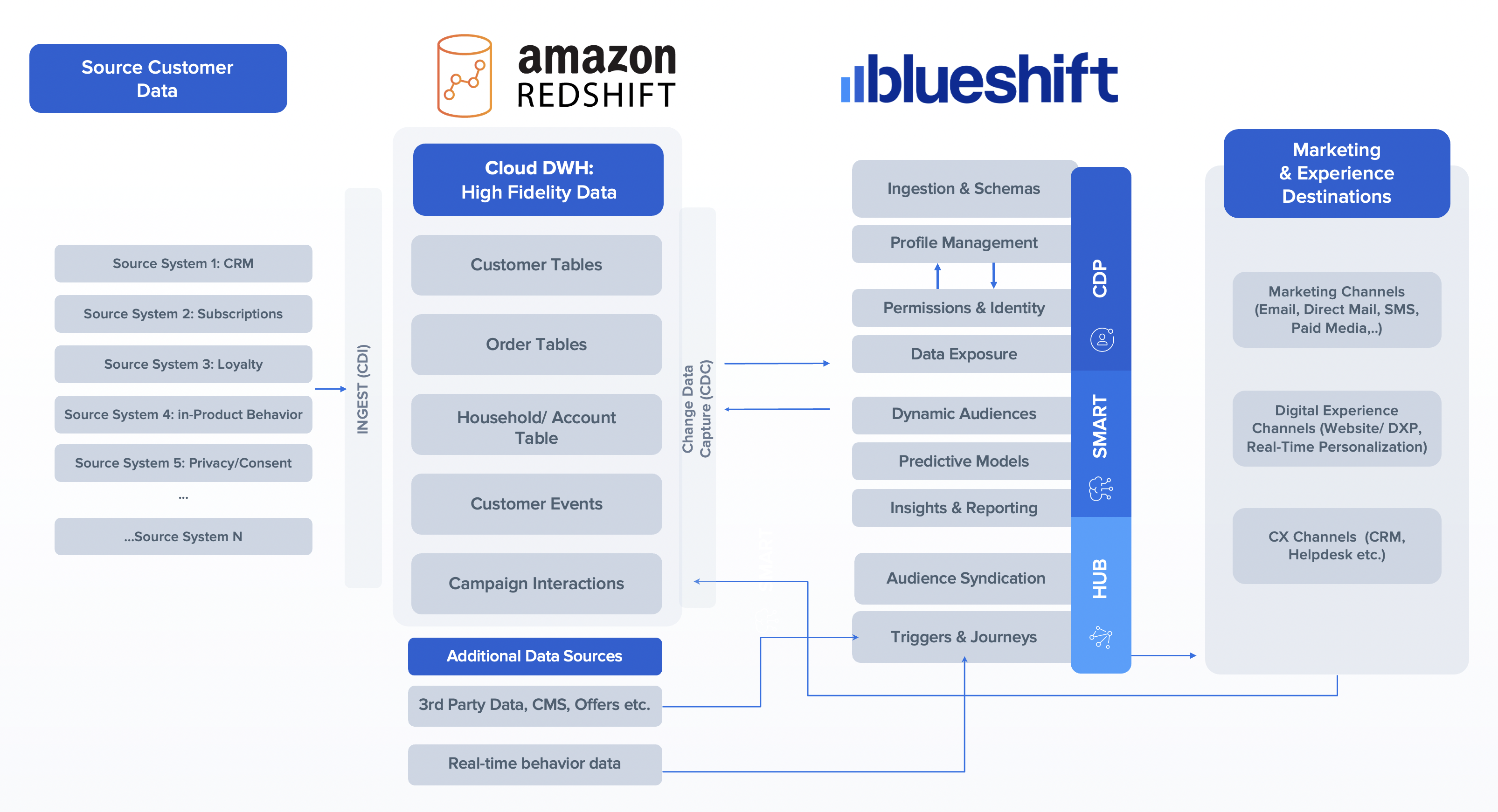
Prerequisites
In this section, we describe the requirements of the integration solution between the two infrastructures. A typical data implementation with customers involves data from Amazon Redshift ingesting into the Blueshift CDP environment. This ingestion mechanism must accommodate different data types, such as the following:
- Customer CRM data (user identifiers and various CRM fields). A typical range for data volume to be supported for this data type is 50–500 GB ingested once initially.
- Real-time behavior or events data (for example, playing or pausing a movie).
- Transactions data, such as subscription purchases. Typical data volumes ingested daily for events and transactions are in the 500 GB – 1 TB range.
- Catalog content (for example, a list of shows or movies for discovery), which is typically about 1 GB in size ingested daily.
The integration also needs to support Blueshift’s CDP platform environment to export data to Amazon Redshift. This includes data such as campaign activities like emails being viewed, which can run into tens of TB, and segment or user exports to support a list of users that are part of a segment definition, typically 50–500 GB exported daily.
Integrate Amazon Redshift with data applications
Amazon Redshift provides several ways to quickly integrate data applications.
For the initial data loads, Blueshift uses Redshift S3 UNLOAD to dump Amazon Redshift data into Amazon Simple Storage Service (Amazon S3). Blueshift natively uses Amazon S3 as a persistent object store and supports bulk ingestion and export from Amazon S3. Data loads from Amazon S3 are ingested in parallel and cut down on data load times, enabling Blueshift clients to quickly onboard.
For incremental data ingestion, Blueshift data import jobs track the last time an import was run, and import new rows of data that have been added or updated since the previous import ran. Blueshift stays in sync with changes (updates or inserts) to the Amazon Redshift data warehouse using the Redshift Data API. Blueshift uses the last\_updated\_at column in Amazon Redshift tables to determine new or updated rows and subsequently ingest those using the Redshift Data API. Blueshift’s data integration cron job syncs data in near-real time using the Redshift Data API by polling for updates on a regular cadence (for example, every 10 minutes, hourly, or daily). The cadence can be tuned depending on data freshness requirements.
The following table summarizes the integration types.
| Integration type | Integration mechanism | Advantage |
| Initial data ingestion from Amazon Redshift to Blueshift | Redshift S3 UNLOAD command | Initial data is exported from Amazon Redshift via Amazon S3 to allow faster parallel loads into Blueshift using the Amazon Redshift UNLOAD command. |
| Incremental data ingestion from Amazon Redshift to Blueshift | Redshift Data API | Incremental data changes are synchronized using the Redshift Data API in near-real time. |
| Data export from Blueshift to Amazon Redshift | Redshift S3 COPY command | Blueshift natively stores campaign activity and segment data in Amazon S3, which is loaded into Amazon Redshift using the Redshift S3 COPY command. |
Redshift supports numerous out-of-the-box mechanisms to provide data access. Blueshift was able to cut down the data onboarding time for clients by using a hybrid approach of integrating with Amazon Redshift with Redshift S3 UNLOAD, the Redshift Data API, and Redshift S3 COPY. Blueshift is able to cut down the initial data load time, as well as be updated in near-real time with changes in Amazon Redshift and vice versa.
Conclusion
In this post, we showed how Blueshift integrated with the Redshift Data API to ingest customer data. This integration was seamless and demonstrated how straightforward the Redshift Data API makes integration with external applications, such as Blueshift’s CDP environment for marketing, with Amazon Redshift. The outlined use cases in this post are just a few examples of how to use the Redshift Data API to simplify interactions between users and Amazon Redshift clusters.
Now go build and integrate Amazon Redshift with Blueshift.
About the authors
 Vijay Chittoor is the CEO & co-founder of Blueshift. Vijay has a wealth of experience in AI, marketing technology and e-commerce domains. Vijay was previously the co-founder & CEO of Mertado (acquired by Groupon to become Groupon Goods), and an early team member at Kosmix (acquired by Walmart to become @WalmartLabs). A former consultant with McKinsey & Co., Vijay is a graduate of Harvard Business School’s MBA Program. He also holds Bachelor’s and Master’s degrees in Electrical Engineering from the Indian Institute of Technology, Bombay.
 Mehul Shah is co-Founder & CTO at Blueshift. Previously, he was a co-founder & CTO at Mertado, which was acquired by Groupon to become Groupon Goods. Mehul was an early employee at Kosmix that was acquired by Walmart to become @WalmartLabs. Mehul is a Y Combinator alumni and a graduate of University of Southern California. Mehul is a co-inventor of 12+ patents, and coaches a middle school robotics team.
 Manohar Vellala is a Senior Solutions Architect at AWS working with digital native customers on their cloud native journey. He is based in San Francisco Bay Area and is passionate about helping customers build modern applications that can take the full advantage of the cloud. Prior to AWS he worked at H2O.ai where he helped customers build ML models. His interests are Storage, Data Analytics and AI/ML.
 Prashant Tyagi joined AWS in September 2020, where he now manages the solutions architecture team focused on enabling digital native businesses. Prashant worked previously at ThermoFisher Scientific, and GE Digital where he held roles as Sr. Director for their Digital Transformation initiatives. Prashant has enabled digital transformation for customers in the Life Sciences and other industry verticals. He has experience in IoT, Data Lakes and AI/ML technical domains. He lives in the bay area in California.
Amazon Redshift is a fully managed, petabyte-scale, massively parallel data warehouse that offers simple operations and high performance. It makes it fast, simple, and cost-effective to analyze all your data using standard SQL and your existing business intelligence (BI) tools. Today, Amazon Redshift is the most widely used cloud data warehouse.
Dynamic data masking (DDM) support (preview) in Amazon Redshift enables you to simplify the process of protecting sensitive data in your Amazon Redshift data warehouse. You can now use DDM to protect data based on your job role or permission rights and level of data sensitivity through a SQL interface. DDM support (preview) in Amazon Redshift enables you to hide, obfuscate, or pseudonymize column values within the tables in your data warehouse without incurring additional storage costs. It is configurable to allow you to define consistent, format-preserving, and irreversible masked data values.
DDM support (preview) in Amazon Redshift provides a native feature to support your need to mask data for regulatory or compliance requirements, or to increase internal privacy standards. Compared to static data masking where underlying data at rest gets permanently replaced or redacted, DDM support (preview) in Amazon Redshift enables you to temporarily manipulate the display of sensitive data in transit at query time based on user privilege, leaving the original data at rest intact. You control access to data through masking policies that apply custom obfuscation rules to a given user or role. That way, you can respond to changing privacy requirements without altering the underlying data or editing SQL queries.
With DDM support (preview) in Amazon Redshift, you can do the following:
- Define masking policies that apply custom obfuscation policies (for example, masking policies to handle credit card, PII entries, HIPAA or GDPR needs, and more)
- Transform the data at query time to apply masking policies
- Attach masking policies to roles or users
- Attach multiple masking policies with varying levels of obfuscation to the same column in a table and assign them to different roles with priorities to avoid conflicts
- Implement cell-level masking by using conditional columns when creating your masking policy
- Use masking policies to partially or completely redact data, or hash it by using user-defined functions (UDFs)
Here’s what our customers have to say on DDM support(private beta) in Amazon Redshift:
“Baffle delivers data-centric protection for enterprises via a data security platform that is transparent to applications and unique to data security. Our mission is to seamlessly weave data security into every data pipeline. Previously, to apply data masking to an Amazon Redshift data source, we had to stage the data in an Amazon S3 bucket. Now, by utilizing the Amazon Redshift Dynamic Data Masking capability, our customers can protect sensitive data throughout the analytics pipeline, from secure ingestion to responsible consumption reducing the risk of breaches.”
-Ameesh Divatia, CEO & co-founder of Baffle
“EnergyAustralia is a leading Australian energy retailer and generator, with a mission to lead the clean energy transition for customers in a way that is reliable, affordable and sustainable for all. We enable all corners of our business with Data & Analytics capabilities that are used to optimize business processes and enhance our customers’ experience. Keeping our customers’ data safe is a top priority across our teams. In the past, this involved multiple layers of custom built security policies that could make it cumbersome for analysts to find the data they require. The new AWS dynamic data masking feature will significantly simplify our security processes so we continue to keep customer data safe, while also reducing the administrative overhead.”
-William Robson, Data Solutions Design Lead, EnergyAustralia
Use case
For our use case, a retail company wants to control how they show credit card numbers to users based on their privilege. They also don’t want to duplicate the data for this purpose. They have the following requirements:
- Users from Customer Service should be able to view the first six digits and the last four digits of the credit card for customer verification
- Users from Fraud Prevention should be able to view the raw credit card number only if it’s flagged as fraud
- Users from Auditing should be able to view the raw credit card number
- All other users should not be able to view the credit card number
Solution overview
The solution encompasses creating masking policies with varying masking rules and attaching one or more to the same role and table with an assigned priority to remove potential conflicts. These policies may pseudonymize results or selectively nullify results to comply with retailers’ security requirements. We refer to multiple masking policies being attached to a table as a multi-modal masking policy. A multi-modal masking policy consists of three parts:
- A data masking policy that defines the data obfuscation rules
- Roles with different access levels depending on the business case
- The ability to attach multiple masking policies on a user or role and table combination with priority for conflict resolution
The following diagram illustrates how DDM support (preview) in Amazon Redshift policies works with roles and users for our retail use case.
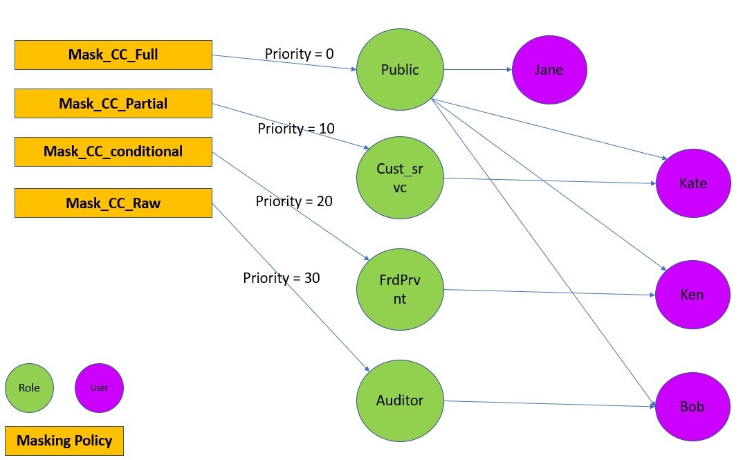
For a user with multiple roles, the masking policy with the highest attachment priority is used. For example, in the following example, Ken is part of the Public and FrdPrvnt role. Because the FrdPrvnt role has a higher attachment priority, card\_number\_conditional\_mask will be applied.

Prerequisites
To implement this solution, you need to complete the following prerequisites:
- Have an AWS account.
- Have an Amazon Redshift cluster provisioned with DDM support (preview) or a serverless workgroup with DDM support (preview).
- Navigate to the provisioned or serverless Amazon Redshift console and choose Create preview cluster.

- In the create cluster wizard, choose the preview track.

- Navigate to the provisioned or serverless Amazon Redshift console and choose Create preview cluster.
- Have Superuser privilege, or the
sys:secadminrole on the Amazon Redshift data warehouse created in step 2.
Preparing the data
To set up our use case, complete the following steps:
- On the Amazon Redshift console, choose Query editor v2 in Explorer.
If you’re familiar with SQL Notebooks, you can download the Jupyter notebook for the demonstration, and import it to quickly get started. - Create the table and populate contents.
- Create users.
Implement the solution
To satisfy the security requirements, we need to make sure that each user sees the same data in different ways based on their granted privileges. To do that, we use user roles combined with masking policies as follows:
- Create user roles and grant different users to different roles:
- Create masking policies:
- Attach the masking policies on the table or column to the user or role:
Test the solution
Let’s confirm that the masking policies are created and attached.
- Check that the masking policies are created with the following code:

- Check that the masking policies are attached:

Now we can test that different users can see the same data masked differently based on their roles.
- Test that the Customer Service agents can only view the first six digits and the last four digits of the credit card number:

- Test that the Fraud Prevention users can only view the raw credit card number when it’s flagged as fraud:
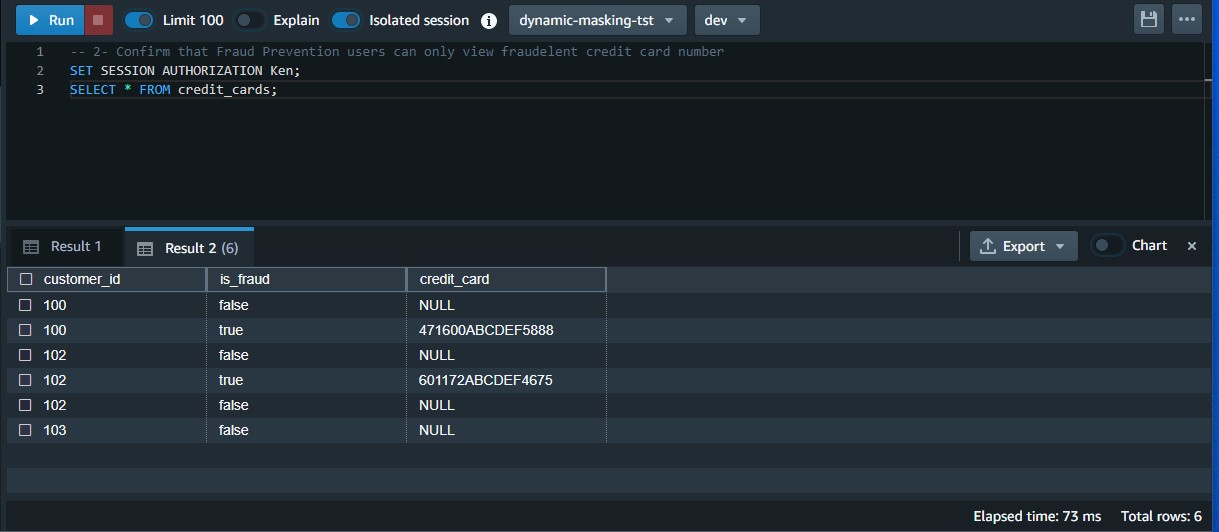
- Test that Auditor users can view the raw credit card number:

- Test that general users can’t view any digits of the credit card number:

Modify the masking policy
To modify an existing masking policy, you must detach it from the role first and then drop and recreate it.
In our use case, the business changed direction and decided that Customer Service agents should only be allowed to view the last four digits of the credit card number.
- Detach and drop the policy:
- Recreate the policy and reattach the policy on the table or column to the intended user or role.Note that this time we created a scalar Python UDF. It’s possible to create a SQL, Python, and Lambda UDF based on your use case.
- Test that Customer Service agents can only view the last four digits of the credit card number:

Clean up
When you’re done with the solution, clean up your resources:
- Detach the masking policies from the table:
- Drop the masking policies:
- Revoke and drop each user and role:
- Drop the function and table:
Considerations and best practices
Consider the following:
- Always create a default policy attached to the public user. If you create a new user, they will always have a minimum policy attached. It will enforce the intended security posture.
- Remember that DDM policies in Amazon Redshift always follow invoker permissions convention, not definer (for more information, refer to Security and privileges for stored procedures ). That being said, the masking policies are applicable based on the user or role running it.
- For best performance, create the masking functions using a scalar SQL UDF, if possible. The performance of scalar UDFs typically goes by the order of SQL to Python to Lambda, in that order. Generally, SQL UDF outperforms Python UDFs and the latter outperforms scalar Lambda UDFs.
- DDM policies in Amazon Redshift are applied ahead of any predicate or join operations. For example, if you’re running a join on a masked column (per your access policy) to an unmasked column, the join will lead to a mismatch. That’s an expected behavior.
- Always detach a masking policy from all users or roles before dropping it.
- As of this writing, the solution has the following limitations:
- You can apply a mask policy on tables and columns and attach it to a user or role, but groups are not supported.
- You can’t create a mask policy on views, materialized views, and external tables.
- The DDM support (preview) in Amazon Redshift is available in following regions: US East (Ohio), US East (N. Virginia), US West (Oregon), Asia Pacific (Tokyo), Europe (Ireland), and Europe (Stockholm).
Performance benchmarks
Based on various tests performed on TPC-H datasets, we’ve found built-in functions to be more performant as compared to functions created externally using scalar Python or Lambda UDFs.
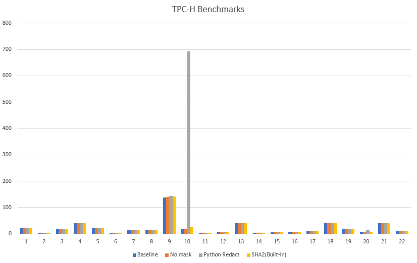
Expand the solution
You can take this solution further and set up a masking policy that restricts SSN and email address access as follows:
- Customer Service agents accessing pre-built dashboards may only view the last four digits of SSNs and complete email addresses for correspondence
- Analysts cannot view SSNs or email addresses
- Auditing services may access raw values for SSNs as well as email addresses
For more information, refer to Use DDM support (preview) in Amazon Redshift for E-mail & SSN Masking.
Conclusion
In this post, we discussed how to use DDM support (preview) in Amazon Redshift to define configuration-driven, consistent, format-preserving, and irreversible masked data values. With DDM support (preview) in Amazon Redshift, you can control your data masking approach using familiar SQL language. You can take advantage of the Amazon Redshift role-based access control capability to implement different levels of data masking. You can create a masking policy to identify which column needs to be masked, and you have the flexibility of choosing how to show the masked data. For example, you can completely hide all the information of the data, replace partial real values with wildcard characters, or define your own way to mask the data using SQL expressions, Python, or Lambda UDFs. Additionally, you can apply a conditional masking based on other columns, which selectively protects the column data in a table based on the values in one or more columns.
We encourage you to create your own user defined functions for various use-cases and accomplish desired security posture using dynamic data masking support in Amazon Redshift.
About the Authors
 Rohit Vashishtha is a Senior Analytics Specialist Solutions Architect at AWS based in Dallas, TX. He has more than 16 years of experience architecting, building, leading, and maintaining big data platforms. Rohit helps customers modernize their analytic workloads using the breadth of AWS services and ensures that customers get the best price/performance with the utmost security and data governance.
 Ahmed Shehata is a Senior Analytics Specialist Solutions Architect at AWS based on Toronto. He has more than two decades of experience helping customers modernize their data platforms. Ahmed is passionate about helping customers build efficient, performant, and scalable analytic solutions.
 Variyam Ramesh is a Senior Analytics Specialist Solutions Architect at AWS based in Charlotte, NC. He is an accomplished technology leader helping customers conceptualize, develop, and deliver innovative analytic solutions.
 Yanzhu Ji is a Product Manager in the Amazon Redshift team. She has experience in product vision and strategy in industry-leading data products and platforms. She has outstanding skill in building substantial software products using web development, system design, database, and distributed programming techniques. In her personal life, Yanzhu likes painting, photography, and playing tennis.
 James Moore is a Technical Lead at Amazon Redshift focused on SQL features and security. His work over the last 10 years has spanned distributed systems, machine learning, and databases. He is passionate about building scalable software that enables customers to solve real-world problems.
Amazon Redshift is a fast, scalable, secure, and fully managed cloud data warehouse that makes it simple and cost-effective to analyze all of your data using standard SQL and your existing business intelligence (BI) tools. Tens of thousands of customers today rely on Amazon Redshift to analyze exabytes of data and run complex analytical queries, making it the most widely used cloud data warehouse.
Data ingestion is the process of getting data from the source system to Amazon Redshift. This can be done by using one of many AWS cloud-based ETL tools like AWS Glue, Amazon EMR, or AWS Step Functions, or you can simply load data from Amazon Simple Storage Service (Amazon S3) to Amazon Redshift using the COPY command. A COPY command is the most efficient way to load a table because it uses the Amazon Redshift massively parallel processing (MPP) architecture to read and load data in parallel from a file or multiple files in an S3 bucket.
Now SQL users can easily automate data ingestion from Amazon S3 to Amazon Redshift with a simple SQL command using the Amazon Redshift auto-copy preview feature. COPY statements are triggered and start loading data when Amazon Redshift auto-copy detects new files in the specified Amazon S3 paths. This also ensures end-users have the latest data available in Amazon Redshift shortly after the source data is available.
This post shows you how to easily build continuous file ingestion pipelines in Amazon Redshift using auto-copy when source files are located on Amazon S3 using a simple SQL command. In addition, we show you how to enable auto-copy using copy jobs, how to monitor jobs, considerations, and best practices.
Overview of the auto-copy feature in Amazon Redshift
The auto-copy feature in Amazon Redshift simplifies automatic data loading from Amazon S3 with a simple SQL command. You can enable Amazon Redshift auto-copy by creating copy jobs. A copy job is a database object that stores, automates, and reuses the COPY statement for newly created files that land in the S3 folder.
The following diagram illustrates this process.
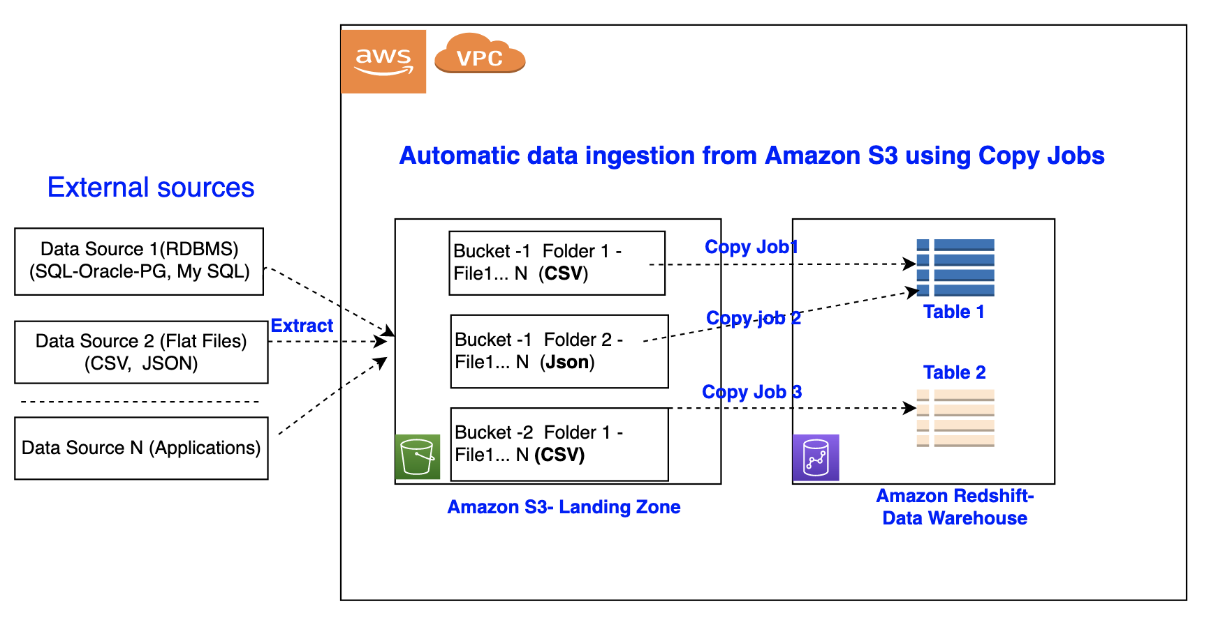
Copy jobs have the following benefits:
- SQL users such as data analysts can now load data from Amazon S3 automatically without having to build a pipeline or using an external framework
- Copy jobs offer continuous and incremental data ingestion from an Amazon S3 location without the need to implement a custom solution
- This functionality comes at no additional cost
- Existing COPY statements can be converted into copy jobs by appending the
JOB CREATE<job\_name> parameter - It keeps track of all loaded files and prevents data duplication
- It can be easily set up using a simple SQL statement and any JDBC or ODBC client
Prerequisites
To get started with auto-copy preview, you need the following prerequisites:
- An AWS account
- An Amazon Redshift cluster with a maintenance track of
PREVIEW\_AUTOCOPY\_2022


The Amazon Redshift auto-copy support from Amazon S3 is available as a preview for provisioned clusters in the following AWS Regions: US East (Ohio), US East (N. Virginia), US West (Oregon), Asia Pacific (Tokyo), Europe (Ireland), and Europe (Stockholm). Please note that for the preview track, restore from snapshot is not supported.
You can refer to the SQL notebook redshift-auto-copy-preview-demo-sql-notebook.ipynb for the SQL statements used in this post.
Set up copy jobs
In this section, we demonstrate how to automate data loading of files from Amazon S3 into Amazon Redshift. With the existing COPY syntax, we add the JOB CREATE parameter to perform a one-time setup for automatic file ingestion. See the following code:
Auto ingestion is enabled by default on copy jobs.
Automate ingestion from a single data source
With a copy job, you can automate ingestion from a single data source by creating one job and specifying the path to the S3 objects that contain the data. The S3 object path can reference a set of folders that have the same key prefix.
In this example, we have multiple files that are being loaded on a daily basis containing the sales transactions across all the stores in the US. Each day’s sales transactions are loaded to their own folder in Amazon S3.
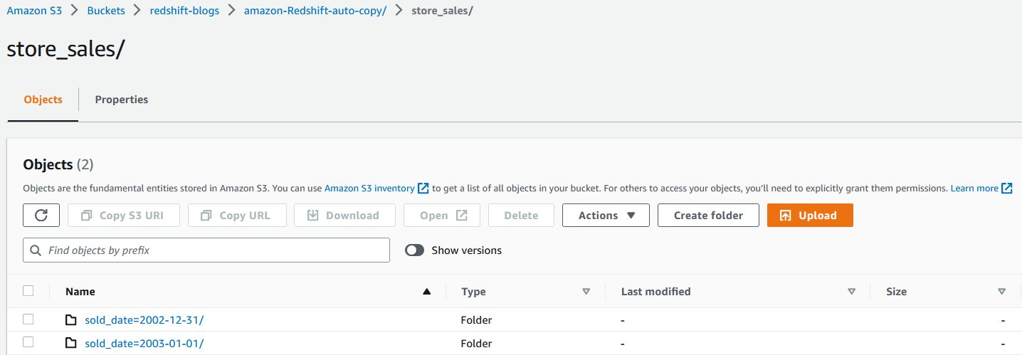
Each folder contains multiple gzip-compressed files.
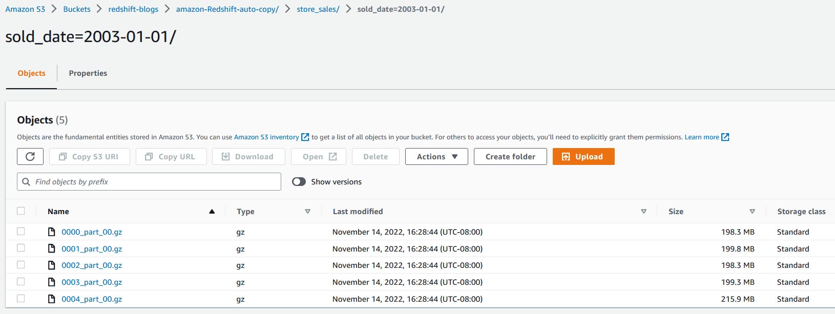
The following code creates the store\_sales table:
Next, we create the copy job to automatically load the gzip-compressed files into the store\_sales table:
When the copy job is created, it automatically loads the existing gzip-compressed files located in the S3 object path specified in the command to the store\_sales table.
Let’s run a query to get the daily total of sales transactions across all the stores in the US:
The output shown comes from the transactions sold on 2002-12-31 and 2003-01-01, respectively.
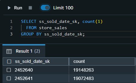
The following day, incremental sales transactions data are loaded to a new folder in the same S3 object path.
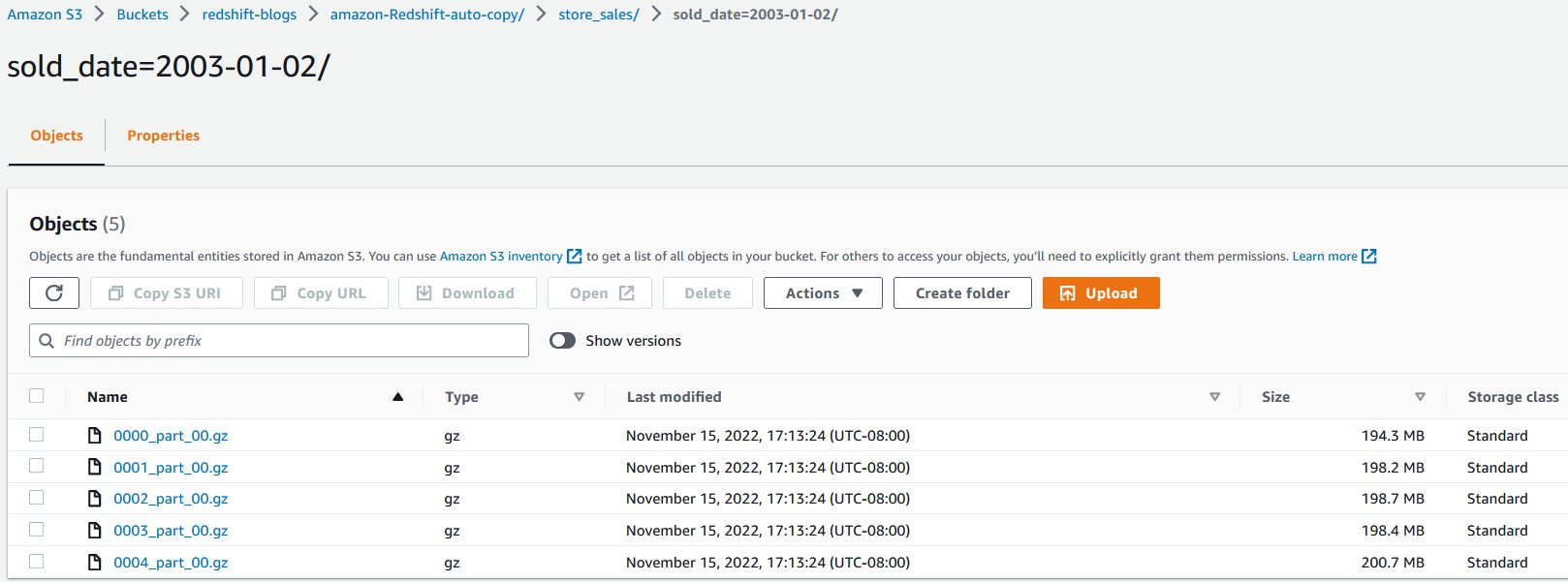
As new files arrive to the same S3 object path, the copy job automatically loads the unprocessed files to the store\_sales table in an incremental fashion.
All new sales transactions for 2003-01-02 are automatically ingested, which can be verified by running the following query:

Automate ingestion from multiple data sources
We can also load an Amazon Redshift table from multiple data sources. When using a pub/sub pattern where multiple S3 buckets populate data to an Amazon Redshift table, you have to maintain multiple data pipelines for each source/target combination. With new parameters in the COPY command, this can be automated to handle data loads efficiently.
In the following example, the Customer\_1 folder has Green Cab Company sales data, and the Customer\_2 folder has Red Cab Company sales data. We can use the COPY command with the JOB parameter to automate this ingestion process.
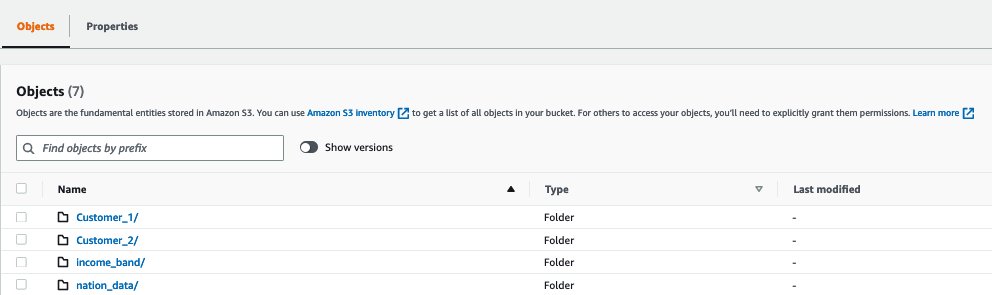
The following screenshot shows sample data stored in files. Each folder has similar data but for different customers.

The target for these files in this example is the Amazon Redshift table cab\_sales\_data.
Define the target table cab\_sales\_data:
You can define two copy jobs as shown in the following code to handle and monitor ingestion of sales data belonging to different customers , in our case Customer\_1 and Customer\_2. These jobs monitor the Customer\_1 and Customer\_2 folders and load any new files that are added here.
Each customer is assigned its own vendorid, as shown in the following output:

Manually run a copy job
There might be scenarios wherein the copy job needs to be paused, meaning it needs to stop looking for new files, for example, to fix a corrupted data pipeline at the data source.
In that case, either use the COPY JOB ALTER command to set AUTO to OFF or create a new COPY JOB with AUTO OFF. Once this is set, auto copy will no longer look for new files.
If in case required, users can manually invoke COPY JOB which will do the work and ingest if any new files found.
COPY JOB RUN <Copy Job Name>
You can disable “AUTO ON” in the existing copy job using the following command:
COPY JOB ALTER <Copy Job Name> AUTO OFF
The following table compares the syntax and data duplication between a regular copy statement and the new auto-copy job.
| . | Copy | Auto-Copy Job (preview) |
| Syntax | COPY <table-name> | COPY <table-name> |
| Data Duplication | If it is run multiple times against the same S3 folder, it will load the data again, resulting in data duplication. | It will not load the same file twice, preventing data duplication. |
For the copy job preview, support on other data formats will be expanded.
Error handling and monitoring for copy jobs
Copy jobs continuously monitor the S3 folder specified during job creation and perform ingestion whenever new files are created. New files created under the S3 folder are loaded exactly once to avoid data duplication.
By default, if there are any data or format issues with the specific files, the copy job will fail to ingest the files with a load error and log details to the system tables. The copy job will remain AUTO ON with new data files and will continue to ignore previously failed files.
Amazon Redshift provides the following system tables for users to monitor or troubleshoot copy jobs as needed:
- List copy jobs – Use SYS\_COPY\_JOB to list all the copy jobs stored in the database:

- Get a summary of a copy job – Use the SYS\_LOAD\_HISTORY view to get the aggregate metrics of a copy job operation by specifying the
copy\_job\_id. It shows the aggregate metrics of all the files that have been processed by a copy job.

- Get details of a copy job – Use STL\_LOAD\_COMMITS to get the status and details of each file that was processed by a copy job:

- Get exception details of a copy job – Use STL\_LOAD\_ERRORS to get the details of files that failed to ingest from a copy job:

Copy job best practices
In a copy job, when a new file is detected and ingested (automatically or manually), Amazon Redshift stores the file name and doesn’t run this specific job when a new file is created with the same file name.
The following are the recommended best practices when working with files using the copy job:
- Use unique file names for each file in a copy job (for example,
2022-10-15-batch-1.csv). However, you can use the same file name as long as it’s from different copy jobs:- job\_customerA\_sales –
s3://redshift-blogs/sales/customerA/2022-10-15-sales.csv - job\_customerB\_sales –
s3://redshift-blogs/sales/customerB/2022-10-15-sales.csv
- job\_customerA\_sales –
- Do not update file contents. Do not overwrite existing files. Changes in existing files will not be reflected to the target table. The copy job doesn’t pick up updated or overwritten files, so make sure they’re renamed as new file names for the copy job to pick up.
- Run regular COPY statements (not a job) if you need to ingest a file that was already processed by your copy job. (COPY without a copy job doesn’t track loaded files.) For example, this is helpful in scenarios where you don’t have control of the file name and the initial file received failed. The following figure shows a typical workflow in this case.
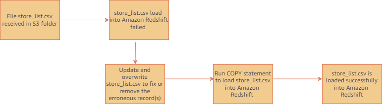
- Delete and recreate your copy job if you want to reset file tracking history and start over.
Copy job considerations
During the preview, here are the main things to consider when using auto-copy:
- The copy job must be created using an empty S3 folder (no existing files)
- The following features are unsupported:
- MAXERROR parameter
- manifest files
- key-based access control
- columnar data format (Parquet, ORC, RCFile, SequenceFile)
- use of
IAM\_ROLEdefault
For additional details on other considerations for auto-copy preview, refer to the AWS documentation.
Customer feedback
GE Aerospace is a global provider of jet engines, components, and systems for commercial and military aircraft. The company has been designing, developing, and manufacturing jet engines since World War I.
“GE Aerospace uses AWS analytics and Amazon Redshift to enable critical business insights that drive important business decisions. With the support for auto-copy from Amazon S3, we can build simpler data pipelines to move data from Amazon S3 to Amazon Redshift. This accelerates our data product teams’ ability to access data and deliver insights to end users. We spend more time adding value through data and less time on integrations.”
– Alcuin Weidus Sr Principal Data Architect at GE Aerospace
Conclusion
This post demonstrated how to automate data load from Amazon S3 to Amazon Redshift using the auto-copy preview feature. This new functionality helps make Amazon Redshift data ingestion easier than ever, and will allow SQL users to get access to the most recent data using a simple SQL command.
As an analysts or SQL users, you can begin ingesting data to Redshift from Amazon S3 with simple SQL commands and gain access to the most up-to-date data without the need for third-party tools or custom implementation.
About the authors
 Jason Pedreza is an Analytics Specialist Solutions Architect at AWS with data warehousing experience handling petabytes of data. Prior to AWS, he built data warehouse solutions at Amazon.com. He specializes in Amazon Redshift and helps customers build scalable analytic solutions.
 Nita Shah is an Analytics Specialist Solutions Architect at AWS based out of New York. She has been building data warehouse solutions for over 20 years and specializes in Amazon Redshift. She is focused on helping customers design and build enterprise-scale well-architected analytics and decision support platforms.
 Eren Baydemir, a Technical Product Manager at AWS, has 15 years of experience in building customer-facing products and is currently focusing on data lake and file ingestion topics in the Amazon Redshift team. He was the CEO and co-founder of DataRow, which was acquired by Amazon in 2020.
 Eesha Kumar is an Analytics Solutions Architect with AWS. He works with customers to realize the business value of data by helping them build solutions using the AWS platform and tools.
Satish Sathiya is a Senior Product Engineer at Amazon Redshift. He is an avid big data enthusiast who collaborates with customers around the globe to achieve success and meet their data warehousing and data lake architecture needs.
 Hangjian Yuan is a Software Development Engineer at Amazon Redshift. He’s passionate about analytical databases and focuses on delivering cutting-edge streaming experiences for customers.
This is a guest post by AWS Data Hero and co-founder of Conduktor, Stephane Maarek.
Deploying Apache Kafka on AWS is now easier, thanks to Amazon Managed Streaming for Apache Kafka (Amazon MSK). In a few clicks, it provides you with a production-ready Kafka cluster on which you can run your applications and create data streams.
Apache Kafka is an open-source project, and no official user interfaces are available. The lack of visibility into Apache Kafka is a factor in the slow development of applications.
The recent announcement of the Conduktor Platform makes Amazon MSK operations simple, and you can solve Kafka issues end to end with solutions for testing, monitoring, data quality, governance, and security.
You can use the Conduktor Platform to monitor both types of MSK clusters, provisioned and serverless. In this post, we demonstrate how to use AWS Identity and Access Management (IAM) based security to administer our MSK cluster.
Solution overview
We look at how we can deploy the Conduktor Platform on Amazon MSK in a production-ready deployment so you can try it out today.
The solution is fully serverless and customizable. Everything is deployed using AWS CloudFormation templates.
The source code and CloudFormation templates used in this post are available in the GitHub repo.
To implement this solution, we complete the following high-level steps:
- Deploy a CloudFormation template to create our customized Docker image for the Conduktor Platform using AWS CodeBuild.
- Optionally, deploy an MSK cluster in provisioned or serverless mode using a CloudFormation template.
- Deploy the Conduktor Platform as an AWS Fargate container against our MSK cluster using a CloudFormation template.
Create a customized configuration for the Conduktor Platform
The Conduktor Platform uses a YAML configuration file to define the cluster connection endpoints. Therefore, we must create a customized Docker image of the Conduktor Platform that is able to connect to a cluster on Amazon MSK with a customized YAML file. For this, we use CodeBuild, and we store our configuration files in Amazon Simple Storage Service (Amazon S3). The final image is stored in Amazon Elastic Container Registry (Amazon ECR). The following diagram illustrates this workflow.
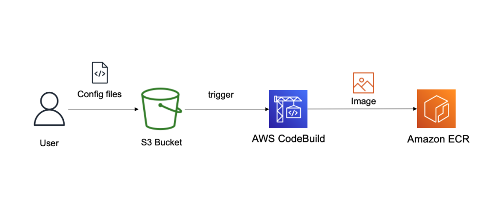
- Deploy the first CloudFormation template to create the following resources:
- An S3 bucket to store our configuration files.
- An ECR repository to store our final Docker image.
- A CodeBuild project to build that Docker image.
- An IAM role and policy to allow CodeBuild to perform the build.
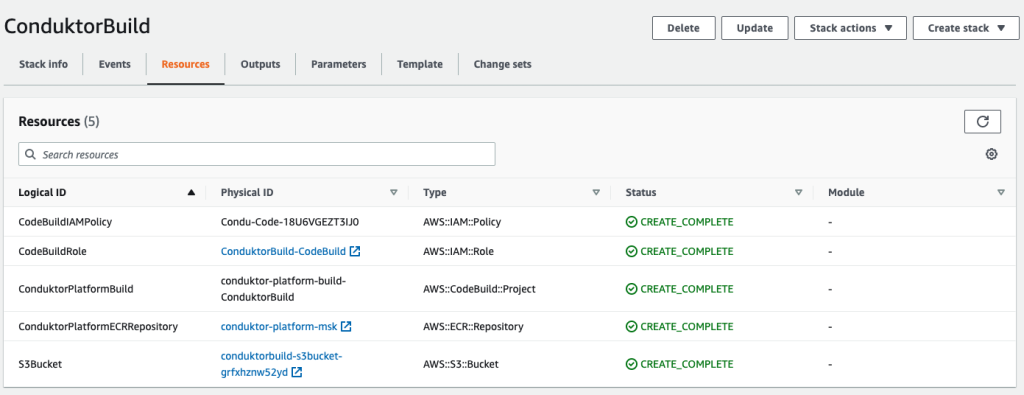
Now we need to upload our files into Amazon S3.
- Upload the following files:
- The file buildspec.yml, which is used by CodeBuild to build our primary Docker image.
- The Dockerfile, which contains instructions on how to build our final Docker image.
- The folder conduktor-platform-config (as is), which contains the configuration files to connect to Amazon MSK.
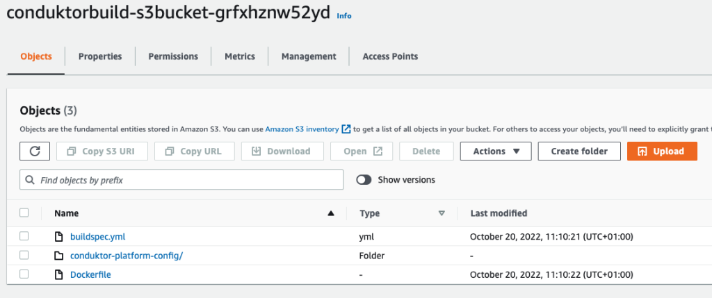
- At this stage, you can customize the
conduktor-platform.yamlfile, allowing you to connect to one MSK cluster:
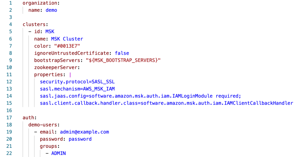
Alternatively, you can connect to multiple MSK clusters or external ones by specifying multiple Kafka bootstrap servers, as shown in the following code. You can also use the same configuration file to specify the schema registry URL, Kafka Connect connection details, and SSO.
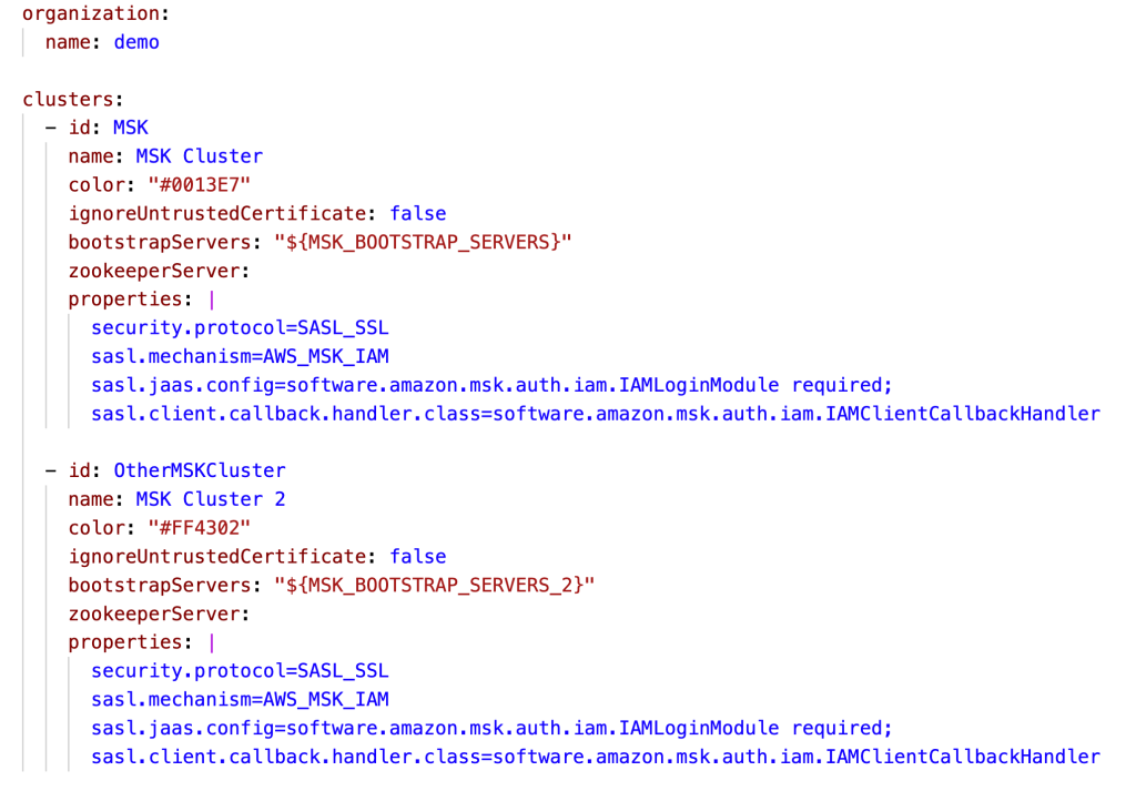
A single-Region Conduktor Platform deployment can work for multi-Region MSK clusters, although natural latency is expected. For latency-sensitive usage, you can deploy this solution in every Region in which you’re using Amazon MSK.
After uploading the files and configurations in your S3 bucket, let’s run CodeBuild to generate a new image.
- On the CodeBuild console, navigate to the project and choose Start build.
The build should complete in about 3 minutes.
The final image is pushed to Amazon ECR thanks to the script hosted in our build-spec.yml script run by CodeBuild. We’re now done with our first step. Your Conduktor Platform setup can now fully connect to your MSK cluster.
Start the MSK cluster
If you already have an MSK cluster set up with IAM access control, you can skip this step. If not, you can create one using the provided CloudFormation template.
From the MSK cluster (the new one or existing one), retrieve two essential pieces of information:
- The bootstrap servers connection string, which is accessed by choosing Client Information
- The MSK security group ID (see the following screenshot)
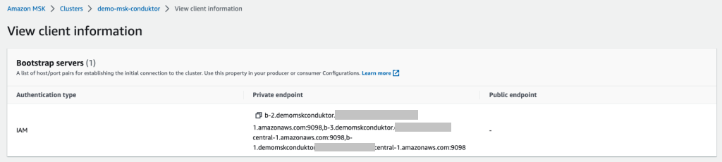
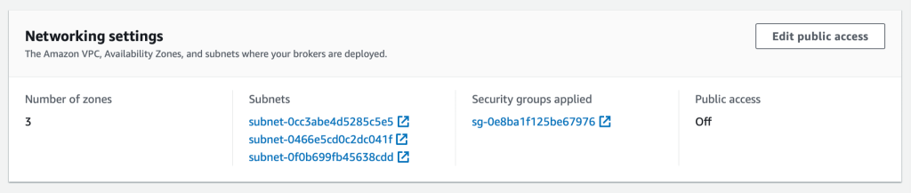
We use IAM access control so that we only need to use IAM policies to connect to our cluster.
If you’re using another security mechanism (such as SASL/SCRAM), you need to modify the Conduktor configuration files with the right properties, upload them back into Amazon S3, and rebuild the Conduktor image using CodeBuild.
Conduktor supports every single Kafka authentication method, including the ones supported by Amazon MSK: IAM access control, mutual TLS authentication, and user name/password using SASL/SCRAM.
Deploy the Conduktor Platform on Amazon ECS with Fargate
The last step is to deploy the Conduktor Platform. For this, we prefer running serverless solutions using Amazon Elastic Container Service (Amazon ECS) with Fargate. This allows you to right-size your containers in the future in case your usage of Conduktor grows over time.
Conduktor stores persistent data in the /var/conduktor file system folder, to store configuration, cache computation results, store logs, and run an internal database (for example, if you start creating data masking rules). For the persistence layer, we use Amazon Elastic File System (Amazon EFS), an elastic network file system that can be mounted on Fargate to provide a persistence layer.
Finally, we expose our Fargate container through an Application Load Balancer, giving us a public static DNS endpoint to expose the Conduktor Platform and giving us complete control over the network security to access the Conduktor Platform. The following diagram illustrates our architecture.
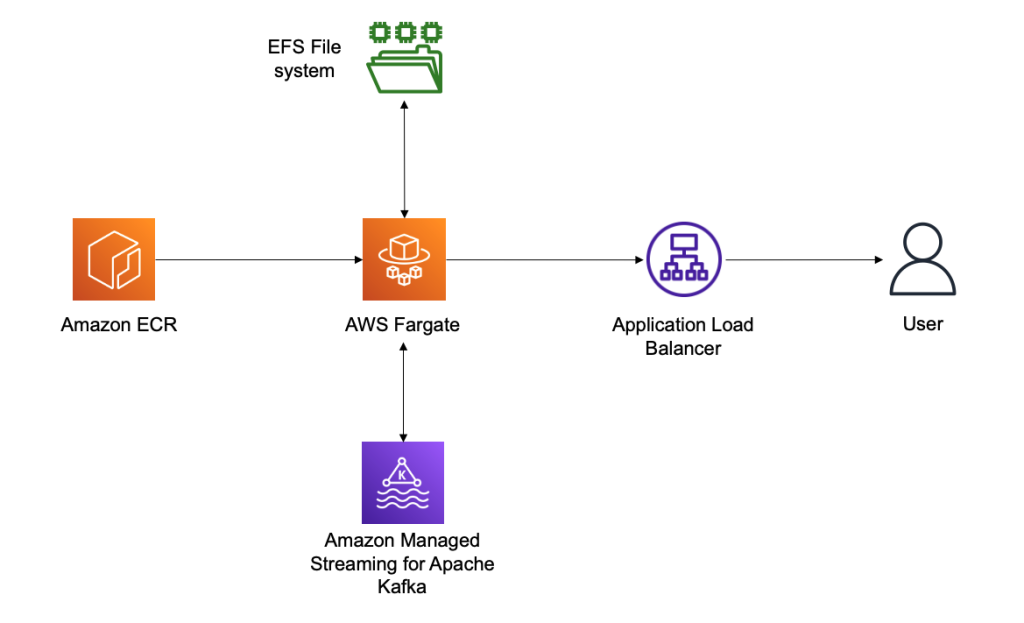
We deploy our last CloudFormation file and specify some important parameters:
- MSKBookstrapServersURL – This parameter is necessary to tell Conduktor which MSK cluster to connect to
- MSKSecurityGroupID – The MSK security group is necessary to allow the template to add a security group ingress rule to it, thereby allowing our ECS task
- PublicSubnetIDs – The public subnet IDs are for your Application Load Balancer
- SubnetIDs – The subnet IDs are for your ECS task and can be the same subnets or private subnets (as long as they have access to the MSK cluster and the other public subnets)
- VpcID – This is the VPC you’re deploying to
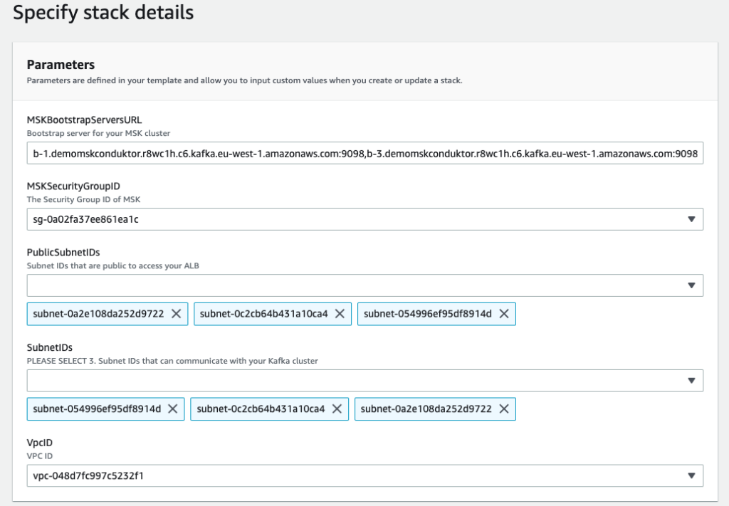
After deploying the template, on the Output tab of the stack, you can find the Application Load Balancer URL.
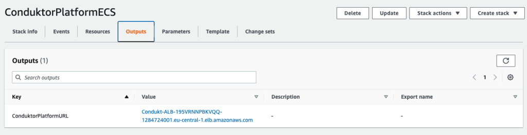
We use this URL and log in to the Conduktor Platform with the user name admin@example.com and password password. These login credentials can be changed using the YAML configuration file, and you can even enable SSO and LDAP.
On the Conduktor console, you can start creating topics, producing data, consuming data, and much more! AWS Glue Schema Registry support is coming soon, and Confluent Schema Registry compatibility is already available.
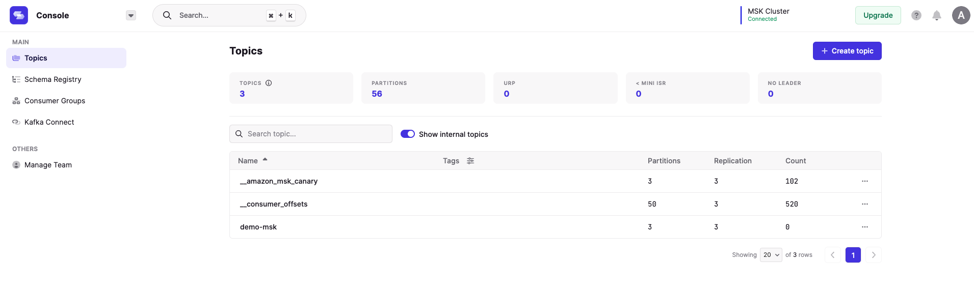
Clean up
To clean up your AWS account, perform the following steps in order:
- Delete the third CloudFormation template (3 – create ECS Service.yaml).
- Delete the second CloudFormation template (2 – create MSK cluster.yaml).
- Empty the contents of your S3 bucket.
- Delete all your images in your ECR repository.
- Delete the first CloudFormation template (1 – base conduktor.yaml).
Conclusion
You can use the Conduktor Platform against as many MSK clusters as desired by editing the file conduktor-platform.yaml. You can even connect to your clusters running elsewhere, for example on Amazon Elastic Compute Cloud (Amazon EC2).
On our roadmap, we’re working on a complete integration with Amazon MSK, including AWS Glue Schema Registry support, Amazon MSK Connect support, and complete monitoring capabilities.
The Conduktor Platform offers a limited free tier with no time limit. Head to Conduktor’s Get Started page and create an account to start using the Platform alongside MSK clusters today.
About the Author
 Stéphane Maarek is the co-founder of Conduktor. He is also the lead instructor on Udemy for learning Apache Kafka and AWS Certifications, having taught these technologies to over 1.5 million learners. Through Conduktor, he wants to democratize access to Apache Kafka and make its usage seamless and enterprise-ready.
Amazon EMR provides a managed service to easily run analytics applications using open-source frameworks such as Apache Spark, Hive, Presto, Trino, HBase, and Flink. The Amazon EMR runtime for Spark and Presto includes optimizations that provide over two times performance improvements over open-source Apache Spark and Presto, so that your applications run faster and at lower cost.
With Amazon EMR release 6.8, you can now use Amazon Elastic Compute Cloud (Amazon EC2) instances such as C6i, M6i, I4i, R6i, and R6id, which use the third-generation Intel Xeon scalable processors. Using these new instances with Amazon EMR improves cost-performance by an additional 5–33% over previous generation instances.
In this post, we describe how we estimated the cost-performance benefit from using Amazon EMR with these new instances compared to using equivalent previous generation instances.
Amazon EMR runtime performance improvements with EC2 I4i instances
We ran TPC-DS 3 TB benchmark queries on Amazon EMR 6.8 using the Amazon EMR runtime for Apache Spark (compatible with Apache Spark 3.3) with five node clusters of I4i instances with data in Amazon Simple Storage Service (Amazon S3), and compared it to equivalent sized I3 instances. We measured performance improvements using the total query runtime and geometric mean of query runtime across the TPC-DS 3 TB benchmark queries.
Our results showed between 36.41–44.39% improvement in total query runtime performance on I4i instance EMR clusters compared to equivalent I3 instance EMR clusters, and between 36–45.2% improvement in geometric mean. To measure cost improvement, we added up the Amazon EMR and Amazon EC2 cost per instance per hour (on-demand) and multiplied it by the total query runtime. Note that I4i 32XL instances were not benchmarked because I3 instances don’t have the 32 XL size available. We observed between 22.56–33.1% reduced instance hour cost on I4i instance EMR clusters compared to equivalent I3 instance EMR clusters to run the TPC-DS benchmark queries. All TPC-DS queries ran faster on I4i instance clusters compared to I3 instance clusters.
The following table shows the results from running TPC-DS 3 TB benchmark queries using Amazon EMR 6.8 over equivalent I3 and I4i instance EMR clusters.
| Instance Size | 16 XL | 8 XL | 4 XL | 2 XL | XL |
| Number of core instances in EMR cluster | 5 | 5 | 5 | 5 | 5 |
| Total query runtime on I3 (seconds) | 4752.15457 | 4506.43694 | 7110.03042 | 11853.40336 | 21333.05743 |
| Total query runtime on I4I (seconds) | 2642.77407 | 2812.05517 | 4415.0023 | 7537.52779 | 12981.20251 |
| Total query runtime improvement with I4I | 44.39% | 37.60% | 37.90% | 36.41% | 39.15% |
| Geometric mean query runtime on I3 (sec) | 34.99551 | 29.14821 | 41.53093 | 60.8069 | 95.46128 |
| Geometric mean query runtime on I4I (sec) | 19.17906 | 18.65311 | 25.66263 | 38.13503 | 56.95073 |
| Geometric mean query runtime improvement with I4I | 45.20% | 36.01% | 38.21% | 37.29% | 40.34% |
| EC2 I3 instance price ($ per hour) | $4.990 | $2.496 | $1.248 | $0.624 | $0.312 |
| EMR I3 instance price ($ per hour) | $0.270 | $0.270 | $0.270 | $0.156 | $0.078 |
| (EC2 + EMR) I3 instance price ($ per hour) | $5.260 | $2.766 | $1.518 | $0.780 | $0.390 |
| Cost of running on I3 ($ per instance) | $6.943 | $3.462 | $2.998 | $2.568 | $2.311 |
| EC2 I4I instance price ($ per hour) | $5.491 | $2.746 | $1.373 | $0.686 | $0.343 |
| EMR I4I price ($ per hour per instance) | $1.373 | $0.687 | $0.343 | $0.172 | $0.086 |
| (EC2 + EMR) I4I instance price ($ per hour) | $6.864 | $3.433 | $1.716 | $0.858 | $0.429 |
| Cost of running on I4I ($ per instance) | $5.039 | $2.681 | $2.105 | $1.795 | $1.546 |
| Total cost reduction with I4I including performance improvement | -27.43% | -22.56% | -29.79% | -30.09% | -33.10% |
The following graph shows per query improvements we observed on I4i 2XL instances with EMR Runtime for Spark on Amazon EMR version 6.8 compared to equivalent I3 2XL instances for the TPC-DS 3 TB benchmark.

Amazon EMR runtime performance improvements with EC2 M6i instances
M6i instances showed a similar performance improvement while running Apache Spark workloads compared to equivalent M5 instances. Our test results showed between 13.45–29.52% improvement in total query runtime for seven different instance sizes within the instance family, and between 7.98–25.37% improvement in geometric mean. On cost comparison, we observed 7.98–25.37% reduced instance hour cost on M6i instance EMR clusters compared to M5 EMR instance clusters to run the TPC-DS benchmark queries.
The following table shows the results from running TPC-DS 3 TB benchmark queries using Amazon EMR 6.8 over equivalent M6i and M5 instance EMR clusters.
| Instance Size | 24 XL | 16 XL | 12 XL | 8 XL | 4 XL | 2 XL | XL |
| Number of core instances in EMR cluster | 5 | 5 | 5 | 5 | 5 | 5 | 5 |
| Total query runtime on M5 (seconds) | 4027.58043 | 3782.10766 | 3348.05362 | 3516.4308 | 5621.22532 | 10075.45109 | 17278.15146 |
| Total query runtime on M6I (seconds) | 3106.43834 | 2665.70607 | 2714.69862 | 3043.5975 | 4195.02715 | 8226.88301 | 14515.50394 |
| Total query runtime improvement with M6I | 22.87% | 29.52% | 18.92% | 13.45% | 25.37% | 18.35% | 15.99% |
| Geometric mean query runtime M5 (sec) | 30.45437 | 28.5207 | 23.95314 | 23.55958 | 32.95975 | 49.43178 | 75.95984 |
| Geometric mean query runtime M6I (sec) | 23.76853 | 19.21783 | 19.16869 | 19.9574 | 24.23012 | 39.09965 | 60.79494 |
| Geometric mean query runtime improvement with M6I | 21.95% | 32.62% | 19.97% | 15.29% | 26.49% | 20.90% | 19.96% |
| EC2 M5 instance price ($ per hour) | $4.61 | $3.07 | $2.30 | $1.54 | $0.77 | $0.38 | $0.19 |
| EMR M5 instance price ($ per hour) | $0.27 | $0.27 | $0.27 | $0.27 | $0.19 | $0.10 | $0.05 |
| (EC2 + EMR) M5 instance price ($ per hour) | $4.88 | $3.34 | $2.57 | $1.81 | $0.96 | $0.48 | $0.24 |
| Cost of running on M5 ($ per instance) | $5.46 | $3.51 | $2.39 | $1.76 | $1.50 | $1.34 | $1.15 |
| EC2 M6I instance price ($ per hour) | $4.61 | $3.07 | $2.30 | $1.54 | $0.77 | $0.38 | $0.19 |
| EMR M6I price ($ per hour per instance) | $1.15 | $0.77 | $0.58 | $0.38 | $0.19 | $0.10 | $0.05 |
| (EC2 + EMR) M6I instance price ($ per hour) | $5.76 | $3.84 | $2.88 | $1.92 | $0.96 | $0.48 | $0.24 |
| Cost of running on M6I ($ per instance) | $4.97 | $2.84 | $2.17 | $1.62 | $1.12 | $1.10 | $0.97 |
| Total cost reduction with M6I including performance improvement | -8.92% | -19.02% | -9.28% | -7.98% | -25.37% | -18.35% | -15.99% |
Amazon EMR runtime performance improvements with EC2 R6i instances
R6i instances showed a similar performance improvement while running Apache Spark workloads compared to equivalent R5 instances. Our test results showed between 14.25–32.23% improvement in total query runtime for six different instance sizes within the instance family, and between 16.12–36.5% improvement in geometric mean. R5.xlarge instances didn’t have sufficient memory to run TPC-DS benchmark queries, and weren’t included in this comparison. On cost comparison, we observed 5.48–23.5% reduced instance hour cost on R6i instance EMR clusters compared to R5 EMR instance clusters to run the TPC-DS benchmark queries.
The following table shows the results from running TPC-DS 3 TB benchmark queries using Amazon EMR 6.8 over equivalent R6i and R5 instance EMR clusters.
| Instance Size | 24 XL | 16 XL | 12 XL | 8 XL | 4 XL | 2XL |
| Number of core instances in EMR cluster | 5 | 5 | 5 | 5 | 5 | 5 |
| Total query runtime on R5 (seconds) | 4024.4737 | 3715.74432 | 3552.97298 | 3535.69879 | 5379.73168 | 9121.41532 |
| Total query runtime on R6I (seconds) | 2865.83169 | 2518.24192 | 2513.4849 | 3031.71973 | 4544.44854 | 6977.9508 |
| Total query runtime improvement with R6I | 28.79% | 32.23% | 29.26% | 14.25% | 15.53% | 23.50% |
| Geometric mean query runtime R5 (sec) | 30.59066 | 28.30849 | 25.30903 | 23.85511 | 32.33391 | 47.28424 |
| Geometric mean query runtime R6I (sec) | 21.87897 | 17.97587 | 17.54117 | 20.00918 | 26.6277 | 34.52817 |
| Geometric mean query runtime improvement with R6I | 28.48% | 36.50% | 30.69% | 16.12% | 17.65% | 26.98% |
| EC2 R5 instance price ($ per hour) | $6.0480 | $4.0320 | $3.0240 | $2.0160 | $1.0080 | $0.5040 |
| EMR R5 instance price ($ per hour) | $0.2700 | $0.2700 | $0.2700 | $0.2700 | $0.2520 | $0.1260 |
| (EC2 + EMR) R5 instance price ($ per hour) | $6.3180 | $4.3020 | $3.2940 | $2.2860 | $1.2600 | $0.6300 |
| Cost of running on R5 ($ per instance) | $7.0630 | $4.4403 | $3.2510 | $2.2452 | $1.8829 | $1.5962 |
| EC2 R6I instance price ($ per hour) | $6.0480 | $4.0320 | $3.0240 | $2.0160 | $1.0080 | $0.5040 |
| EMR R6I price ($ per hour per instance) | $1.5120 | $1.0080 | $0.7560 | $0.5040 | $0.2520 | $0.1260 |
| (EC2 + EMR) R6I instance price ($ per hour) | $7.5600 | $5.0400 | $3.7800 | $2.5200 | $1.2600 | $0.6300 |
| Cost of running on R6I ($ per instance) | $6.0182 | $3.5255 | $2.6392 | $2.1222 | $1.5906 | $1.2211 |
| Total cost reduction with R6I including performance improvement | -14.79% | -20.60% | -18.82% | -5.48% | -15.53% | -23.50% |
Amazon EMR runtime performance improvements with EC2 C6i instances
C6i instances showed a similar performance improvement while running Apache Spark workloads compared to equivalent C5 instances. Our test results showed between 16.9–58.22% improvement in total query runtime for four different instance sizes within the instance family, and between 20.25–59.59% improvement in geometric mean. Only C6i 24, 12, 4, and 2xlarge sizes were benchmarked because C5 doesn’t have 32, 16 and 8 xlarge sizes. C5.xlarge instances didn’t have sufficient memory to run TPC-DS benchmark queries, and weren’t included in this comparison. On cost comparison, we observed 16.75–50.07% reduced instance hour cost on C6i instance EMR clusters compared to C5 EMR instance clusters to run the TPC-DS benchmark queries.
The following table shows the results from running TPC-DS 3 TB benchmark queries using Amazon EMR 6.8 over equivalent C6i and C5 instance EMR clusters.
| Instance Size * | 24 XL | 12 XL | 4 XL | 2 XL |
| Number of core instances in EMR cluster | 5 | 5 | 5 | 5 |
| Total query runtime on C5 (seconds) | 3435.59808 | 2900.84981 | 5945.12879 | 10173.00757 |
| Total query runtime on C6I (seconds) | 2711.16147 | 2471.86778 | 5195.30093 | 8787.43422 |
| Total query runtime improvement with C6I | 21.09% | 14.79% | 12.61% | 13.62% |
| Geometric mean query runtime C5 (sec) | 25.67058 | 20.06539 | 31.76582 | 46.78632 |
| Geometric mean query runtime C6I (sec) | 20.4458 | 17.14133 | 26.92196 | 39.32622 |
| Geometric mean query runtime improvement with C6I | 20.35% | 14.57% | 15.25% | 15.95% |
| EC2 C5 instance price ($ per hour) | $4.080 | $2.040 | $0.680 | $0.340 |
| EMR C5 instance price ($ per hour) | $0.270 | $0.270 | $0.170 | $0.085 |
| (EC2 + EMR) C5 instance price ($ per hour) | $4.35000 | $2.31000 | $0.85000 | $0.42500 |
| Cost of running on C5 ($ per instance) | $4.15135 | $1.86138 | $1.40371 | $1.20098 |
| EC2 C6I instance price ($ per hour) | $4.0800 | $2.0400 | $0.6800 | $0.3400 |
| EMR C6I price ($ per hour per instance) | $1.02000 | $0.51000 | $0.17000 | $0.08500 |
| (EC2 + EMR) C6I instance price ($ per hour) | $5.10000 | $2.55000 | $0.85000 | $0.42500 |
| Cost of running on C6I ($ per instance) | $3.84081 | $1.75091 | $1.22667 | $1.03741 |
| Total cost reduction with C6I including performance improvement | -7.48% | -5.93% | -12.61% | -13.62% |
Amazon EMR runtime performance improvements with EC2 R6id instances
R6id instances showed a similar performance improvement while running Apache Spark workloads compared to equivalent R5D instances. Our test results showed between 11.8–28.7% improvement in total query runtime for five different instance sizes within the instance family, and between 15.1–32.0% improvement in geometric mean. R6ID 32 XL instances were not benchmarked because R5D instances don’t have these sizes available. On cost comparison, we observed 6.8–11.5% reduced instance hour cost on R6ID instance EMR clusters compared to R5D EMR instance clusters to run the TPC-DS benchmark queries.
The following table shows the results from running TPC-DS 3 TB benchmark queries using Amazon EMR 6.8 over equivalent R6id and R5d instance EMR clusters.
| Instance Size | 24 XL | 16 XL | 12 XL | 8 XL | 4 XL | 2 XL | XL |
| Number of core instances in EMR cluster | 5 | 5 | 5 | 5 | 5 | 5 | 5 |
| Total query runtime on R5D (seconds) | 4054.4492975042 | 3691.7569385583 | 3598.6869168064 | 3532.7398928104 | 5397.5330161574 | 9281.2627059927 | 16862.8766838096 |
| Total query runtime on R6ID (seconds) | 2992.1198446983 | 2633.7131630720 | 2632.3186613402 | 2729.8860537867 | 4583.1040980373 | 7921.9960917943 | 14867.5391541445 |
| Total query runtime improvement with R6ID | 26.20% | 28.66% | 26.85% | 22.73% | 15.09% | 14.65% | 11.83% |
| Geometric mean query runtime R5D (sec) | 31.0238156851 | 28.1432927726 | 25.7532157307 | 24.0596427675 | 32.5800246829 | 48.2306670294 | 76.6771994376 |
| Geometric mean query runtime R6ID (sec) | 22.8681174894 | 19.1282742957 | 18.6161830746 | 18.0498249257 | 25.9500918360 | 39.6580341258 | 65.0947323858 |
| Geometric mean query runtime improvement with R6ID | 26.29% | 32.03% | 27.71% | 24.98% | 20.35% | 17.77% | 15.11% |
| EC2 R5D instance price ($ per hour) | $6.912000 | $4.608000 | $3.456000 | $2.304000 | $1.152000 | $0.576000 | $0.288000 |
| EMR R5D instance price ($ per hour) | $0.270000 | $0.270000 | $0.270000 | $0.270000 | $0.270000 | $0.144000 | $0.072000 |
| (EC2 + EMR) R5D instance price ($ per hour) | $7.182000 | $4.878000 | $3.726000 | $2.574000 | $1.422000 | $0.720000 | $0.360000 |
| Cost of running on R5D ($ per instance) | $8.088626 | $5.002331 | $3.724641 | $2.525909 | $2.132026 | $1.856253 | $1.686288 |
| EC2 R6ID instance price ($ per hour) | $7.257600 | $4.838400 | $3.628800 | $2.419200 | $1.209600 | $0.604800 | $0.302400 |
| EMR R6ID price ($ per hour per instance) | $1.814400 | $1.209600 | $0.907200 | $0.604800 | $0.302400 | $0.151200 | $0.075600 |
| (EC2 + EMR) R6ID instance price ($ per hour) | $9.072000 | $6.048000 | $4.536000 | $3.024000 | $1.512000 | $0.756000 | $0.378000 |
| Cost of running on R6ID ($ per instance) | $7.540142 | $4.424638 | $3.316722 | $2.293104 | $1.924904 | $1.663619 | $1.561092 |
| Total cost reduction with R6ID including performance improvement | -6.78% | -11.55% | -10.95% | -9.22% | -9.71% | -10.38% | -7.42% |
Benchmarking methodology
The benchmark used in this post is derived from the industry-standard TPC-DS benchmark, and uses queries from the Spark SQL Performance Tests GitHub repo with the following fixes applied.
We calculated TCO by multiplying cost per hour by number of instances in the cluster and time taken to run the queries on the cluster. We used the on-demand pricing in the US East (N. Virginia) Region for all instances.
Conclusion
In this post, we described how we estimated the cost-performance benefit from using Amazon EMR with C6i, M6i, I4i, R6i, and R6id, instances compared to using equivalent previous generation instances. Using these new instances with Amazon EMR improves cost-performance by an additional 5–33%.
About the authors
Al MS is a product manager for Amazon EMR at Amazon Web Services.
Kyeonghyun Ryoo is a Software Development Engineer for EMR at Amazon Web Services. He primarily works on designing and building automation tools for internal teams and customers to maximize their productivity. Outside of work, he is a retired world champion in professional gaming who still enjoy playing video games.
Organizations are working towards centralizing their identity and access strategy across all their applications, including on-premises, third-party, and applications on AWS. Many organizations use identity providers (IdPs) based on OIDC or SAML-based protocols like Microsoft Azure Active Directory (Azure AD) and manage user authentication along with authorization centrally. This authorizes users to access Amazon QuickSight assets-analyses, dashboards, folders, and datasets-through centrally managed Azure AD and AWS IAM Identity Center (successor to AWS Single Sign-On).
IAM Identity Center is an authentication process that allows users to sign into multiple applications with a single set of usernames and passwords. IAM Identity Center makes it easy to centrally manage access to multiple AWS accounts and business applications. It provides your workforce with single sign-on (SSO) access to all assigned accounts and applications from one place.
In this post, we walk you through the steps required to configure federated SSO along with automated email sync between QuickSight and Azure AD via IAM Identity Center. We also demonstrate ways System for Cross-domain Identity Management (SCIM) keeps your IAM Identity Center identities in sync with identities from your IdP.
Solution overview
The following is the reference architecture for configuring IAM Identity Center with Azure AD for automated federation to QuickSight and the AWS Management Console.

The following are the steps involved to set up federated SSO from Azure to QuickSight:
- Configure Azure as an IdP in IAM Identity Center.
- Register an IAM Identity Center application in Azure AD.
- Configure the application in Azure AD.
- Enable automatic provisioning of users and groups.
- Enable email syncing for federated users in QuickSight console.
- Create a QuickSight application in IAM Identity Center.
- Add the IAM Identity Center application as a SAML IdP.
- Configure AWS Identity and Access Management (IAM) policies and roles.
- Configure attribute mappings in IAM Identity Center.
- Validate federation to QuickSight from IAM Identity Center.
Prerequisites
To complete this walkthrough, you must have the following prerequisites:
- An Azure AD subscription with Administrator permission.
- QuickSight account subscription with Administrator permission.
- IAM Administrator account.
- IAM Identity Center Administrator account.
Configure Azure as IdP in IAM Identity Center
To configure Azure as an IdP, complete the following steps:
- On the IAM Identity Center console, choose Enable.

- Choose Choose your identity source.

- Select External identity provider to manage all users and groups.
- Choose Next.

- In the Configure external identity provider section, download the service provider metadata file.
- Save the AWS access portal sign-in URL, IAM Identity Center Assertion Consumer Service (ACS) URL, and IAM Identity Center issuer URL.
These are used later in this post.
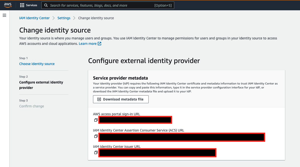
- Leave this tab open in your browser while proceeding to the next steps.
Register an IAM Identity Center application in Azure AD
To register an IAM Identity Center application in Azure AD, complete the following steps:
- Sign in to your Azure portal using an administrator account.
- Under Azure Services, choose Azure AD and under Manage, choose Enterprise applications.

- Choose New application.
- Choose Create your own application.
- Enter a name for the application.
- Select the option Integrate any other application you don’t find in the gallery (Non-gallery).
- Choose Create.

Configure the application in Azure AD
To configure your application, complete the following steps:
- Under Enterprise applications, choose All applications and select the application created in the previous step.
- Under Manage, choose Single Sign-on.
- Choose SAML.

- Choose Single Sign-on to set up SSO with SAML.
- Choose Upload metadata file, and upload the file you downloaded from IAM Identity Center.

- Choose Edit to edit the Basic SAML Configuration section.
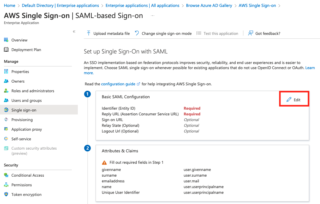
- For Identifier (Entity ID), enter the IAM Identity Center issuer URL.
- For Reply URL (Assertion Consumer Service URL), enter the IAM Identity Center ACS URL.
- Under SAML Signing Certificate, choose Download next to Federation Metadata XML.

We use this XML document in later steps when setting up the SAML provider in IAM and in IAM Identity Center.
- Leave this tab open in your browser while moving to the next steps.
- Switch to the IAM Identity Center tab to complete its setup.
- Under Identity provider metadata, choose IdP SAML metadata and upload the federation metadata XML file you downloaded.

- Review and confirm the changes.

Enable automatic provisioning of users and groups
IAM Identity Center supports System for Cross-domain Identity Management (SCIM) v2.0 standard. SCIM keeps your IAM Identity Center identities in sync with external IdPs. This includes any provisioning, updates, and deprovisioning of users between IdP and IAM Identity Center. To enable SCIM, complete the following steps:
- On the IAM Identity Center console, choose Settings in the navigation pane.
- Next to Automatic provisioning, choose Enable.

- Copy the SCIM endpoint and Access token.
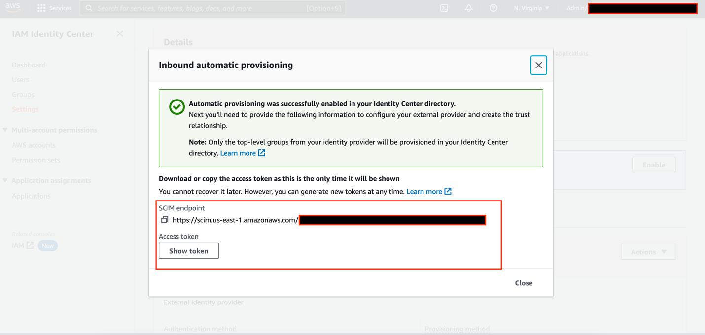
- Switch to the Azure AD tab.
- On the Default Directory Overview page, under Manage, choose Users.

- Choose New user and Create new user(s).
Make sure the user profile has valid information under First name, Last name, and Email attribute.
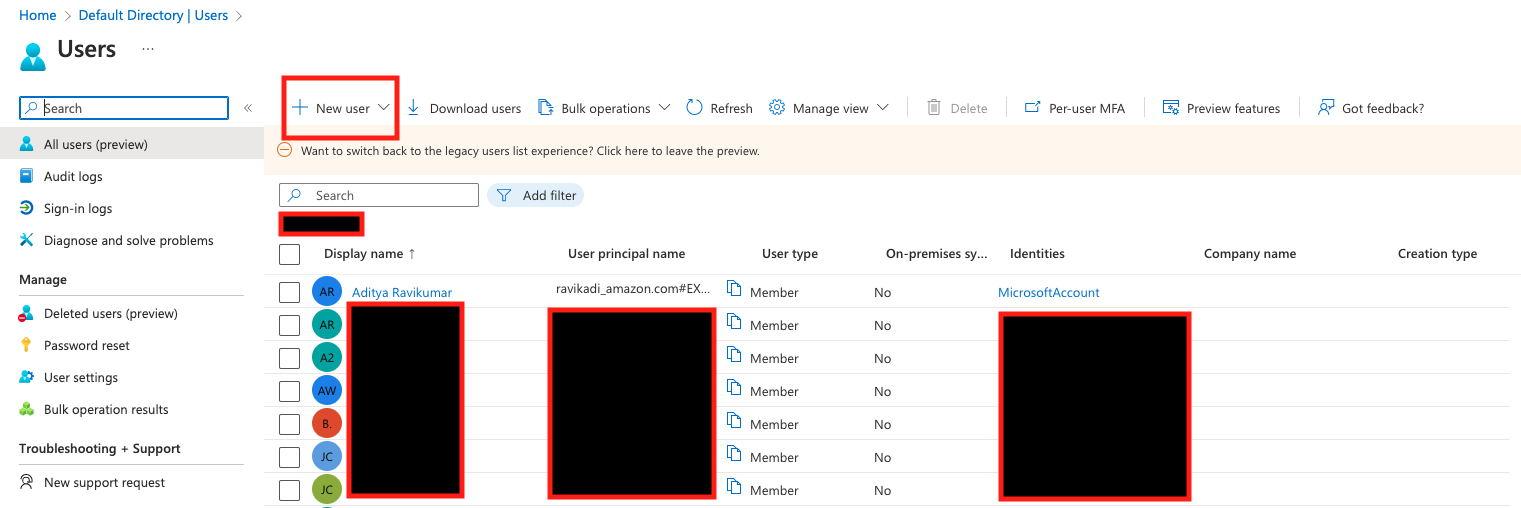
- Under Enterprise applications, choose All applications and select the application you created earlier.
- Under Manage, choose Users and groups.
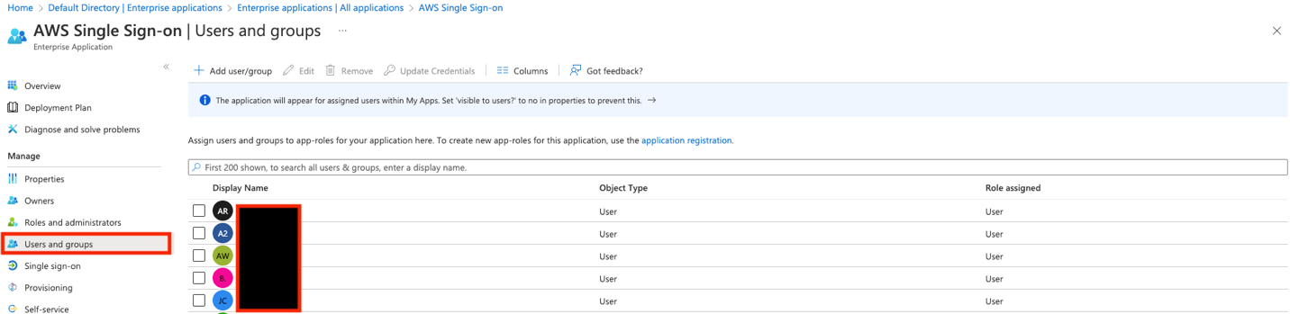
- Choose Add user/group, and select the users you created earlier.
- Choose Assign.
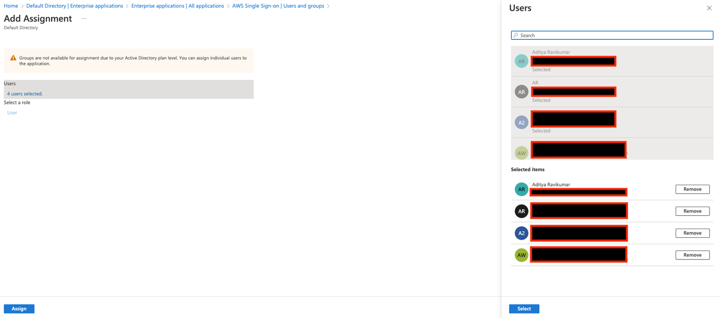
- Under Manage, choose Provisioning and Get started.
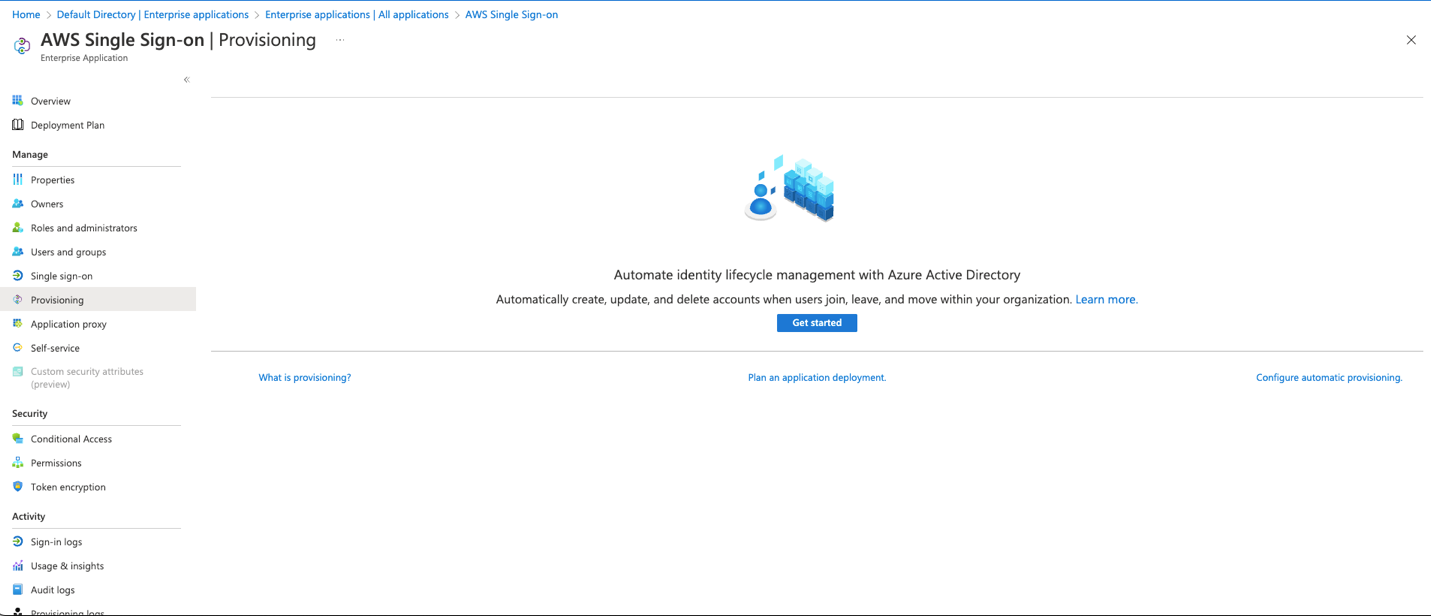
- Choose Provisioning Mode as Automatic.
- For Tenant URL, enter the SCIM endpoint.
- For Secret Token, enter the Access token.
- Choose Test Connection and Save.

- Under Provisioning, choose Start provisioning.

Make sure the user profile has valid information under First name, Last name, and Email attribute. This is the key value for email sync with QuickSight.

On the IAM Identity Center console, under Users, you can now see all the users provisioned from Azure AD.

Enable email syncing for federated users in QuickSight console
Complete the following steps to enable email syncing for federated users:
- Sign in as an admin user to the QuickSight console and choose Manage QuickSight from the user name menu.

- Choose Single sign-on (SSO) in the navigation pane.

- Under Email Syncing for Federated Users, select ON.

Create a QuickSight application in IAM Identity Center
Complete the following steps to create a custom SAML 2.0 application in IAM Identity Center.
- On the IAM Identity Center console, choose Applications in the navigation pane.
- Choose Add application.

- Under Preintegrated applications, search for and choose Amazon QuickSight.
- Choose Next.
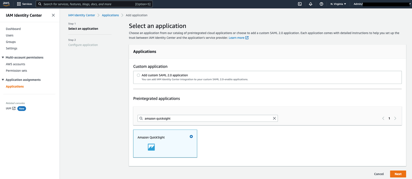
- For Display name, enter a name, such as
Amazon QuickSight. - For Description, enter a description.
- Download the IAM Identity Center SAML metadata file to use later in this post.
- For Application start URL, leave as is.
- For Relay state, enter
https://quicksight.aws.amazon.com. - For Session duration, choose your session duration. The recommended value is 8 hours.
- For Application ACS URL, enter
https://signin.aws.amazon.com/saml. - For Application SAML audience, enter
urn:amazon:webservices. - Choose Submit
After your settings are saved, your application configuration should look similar to the following screenshot.

You can now assign your users to this application, so that the application appears in their IAM Identity Center portal after login.
- On the application page, under Assigned users, choose Assign Users.

- Select your users.
- Optionally, if you want to enable multiple users in your organization to use QuickSight, the fastest and easiest way is to use IAM Identity Center groups.
- Choose Assign Users.

Add the IAM Identity Center application as a SAML IdP
Complete the following steps to configure IAM Identity Center as your SAML IdP:
- Open a new tab in your browser.
- Sign in to the IAM console in your AWS account with admin permissions.
- Choose Identity providers in the navigation pane.
- Choose Add provider.
- Select SAML for Provider type.
- For Provider name, enter
IAM\_Identity\_Center. - Choose Choose File to upload the metadata document you downloaded earlier from the Amazon QuickSight application.
- Choose Add Provider.

- On the summary page, record the value for the provider ARN (
arn:aws:iam::<AccountID>:saml-provider/IAM\_Identity\_Center).
You will use this ARN while configuring claims rules later in this post.
Configure IAM policies
In this step, you create three IAM policies for different role permissions in QuickSight:
QuickSight-Federated-AdminQuickSight-Federated-AuthorQuickSight-Federated-Reader
Use the following steps to set up QuickSight-Federated-Admin policy. This policy grants admin privileges in QuickSight to the federated user:
- On the IAM console, choose Policies in the navigation pane
- Choose Create policy.
- Choose JSON and replace the existing text with the following code:
Ignore the “Missing ARN Region: Add a Region to the quicksight resource ARN” error and continue. Optionally, you could also add a specific AWS region in the ARN.
- Choose Review policy
- For Name enter
QuickSight-Federated-Admin. - Choose Create policy.
- Repeat these steps to create the
QuickSight-Federated-Authorpolicy using the following JSON code to grant author privileges in QuickSight to the federated user:
Ignore the “Missing ARN Region: Add a Region to the quicksight resource ARN” error and continue. Optionally, you could also add a specific AWS region in the ARN.
- Repeat these steps to create the
QuickSight-Federated-Readerpolicy using the following JSON code to grant reader privileges in QuickSight to the federated user:
Ignore the “Missing ARN Region: Add a Region to the quicksight resource ARN” error and continue. Optionally, you could also add a specific AWS region in the ARN.
Configure IAM roles
Next, create roles that your Azure AD and IAM Identity Center users assume when federating into QuickSight. The following steps set up the admin role:
- On the IAM console, choose Roles in the navigation pane.
- Choose Create role.
- For Select type of trusted entity, choose SAML 2.0 federation.
- For SAML provider, choose the provider you created earlier (
IAM\_Identity\_Center). - Select Allow programmatic and AWS Management Console access.
- For Attribute, make sure SAML:aud is selected.
- For Value, make sure
https://signin.aws.amazon.com/samlis selected. - Choose Next.

- Choose the
QuickSight-Federated-AdminIAM policy you created earlier. - Choose Next: Tags.
- Choose Next: Review.
- For Role name, enter
QuickSight-Admin-Role. - For Role description, enter a description.
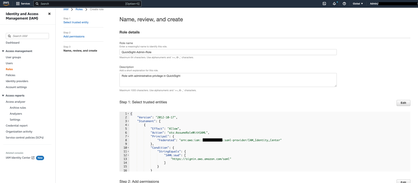
- Choose Create role.
- On the IAM console, in the navigation pane, choose Roles.
- Choose the
QuickSight-Admin-Rolerole you created to open the role’s properties. - Record the role ARN to use later.
- On the Trust relationships tab, choose Edit trust policy.

- For the policy details, enter the following JSON:
- Choose Update Policy.
- Repeat these steps to create the roles
QuickSight-Author-RoleandQuickSight-Reader-Role. Attach theQuickSight-Federated-AuthorandQuickSight-Federated-Readerpolicies to their respectively roles.
Configure attribute mappings in IAM Identity Center
The final step is to configure the attribute mappings in IAM Identity Center. The attributes you map here become part of the SAML assertion that is sent to the QuickSight application. You can choose which user attributes in your application map to corresponding user attributes in your connected directory. For more information, refer to Attribute mappings.
- On IAM Identity Center console, choose Applications in the navigation pane.

- Select the
Amazon QuickSightapplication you created earlier.
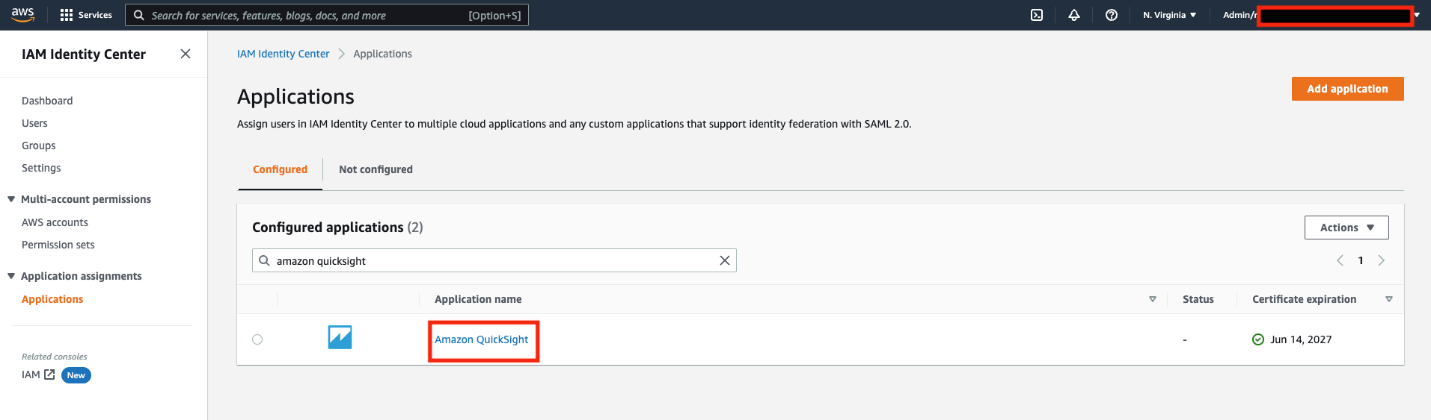
- On the Actions menu, choose Edit attribute mappings.
- Configure the following mappings:
| User attribute in the application | Maps to this string value or user attribute in IAM Identity Center | Format |
Subject | ${user:email} | emailAddress |
https://aws.amazon.com/SAML/Attributes/Role | arn:aws:iam:: <YourAWSAccount ID>:saml-provider/IAM\_Identity\_Center, arn:aws:iam:: <YourAWSAccount ID>:role/QuickSight-Admin-Role | unspecified |
https://aws.amazon.com/SAML/Attributes/RoleSessionName | ${user:email} | unspecified |
https://aws.amazon.com/SAML/Attributes/PrincipalTag:Email | ${user:email} | url |
- Choose Save changes.
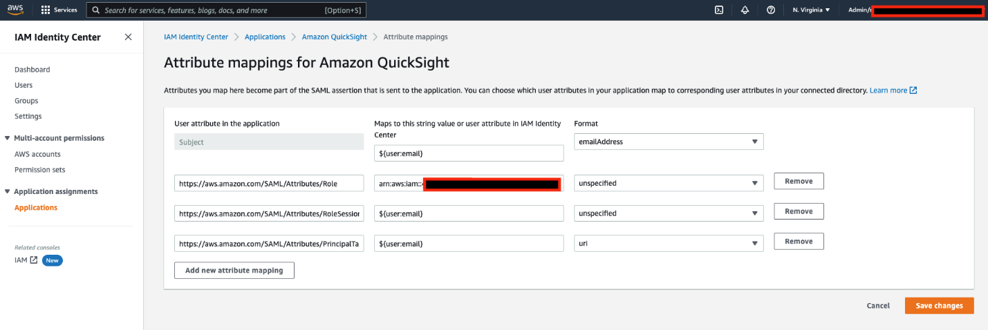
Validate federation to QuickSight from IAM Identity Center
On the IAM Identity Center console, note down the user portal URL available on the Settings page. We suggest you log out of your AWS account first, or open an incognito browser window. Navigate to the user portal URL, sign in with the credentials of an AD user, and choose your QuickSight application.


You’re automatically redirected to the QuickSight console.


Summary
This post provided step-by-step instructions to configure federated SSO with Azure AD as IdP through IAM Identity Center. We also discussed how SCIM keeps your IAM Identity Center identities in sync with identities from your IdP. This includes any provisioning, updating, and deprovisioning of users between your IdP and IAM Identity Center.
If you have any questions or feedback, please leave a comment.
For additional discussions and help getting answers to your questions, check out the QuickSight Community.
About the author
 Aditya Ravikumar is a Solutions Architect at Amazon Web Services. He is based in Seattle, USA. Aditya’s core interests include software development, databases, data analytics and machine learning. He works with AWS customers/partners to provide guidance and technical assistance to transform their business through innovative use of cloud technologies.
Srikanth Baheti is a Specialized World Wide Sr. Solution Architect for Amazon QuickSight. He started his career as a consultant and worked for multiple private and government organizations. Later he worked for PerkinElmer Health and Sciences & eResearch Technology Inc, where he was responsible for designing and developing high traffic web applications, highly scalable and maintainable data pipelines for reporting platforms using AWS services and Serverless computing.
Raji Sivasubramaniam is a Sr. Solutions Architect at AWS, focusing on Analytics. Raji is specialized in architecting end-to-end Enterprise Data Management, Business Intelligence and Analytics solutions for Fortune 500 and Fortune 100 companies across the globe. She has in-depth experience in integrated healthcare data and analytics with wide variety of healthcare datasets including managed market, physician targeting and patient analytics.
In this post, we show how to use Amazon QuickSight and Amazon Athena Federated Query to build dashboards and visualizations on data that is stored in Microsoft Azure Synapse databases.
Organizations today use data stores that are best suited for the applications they build. Additionally, they may also continue to use some of their legacy data stores as they modernize and migrate to the cloud. These disparate data stores might be spread across on-premises data centers and different cloud providers. This presents a challenge for analysts to be able to access, visualize, and derive insights from the disparate data stores.
QuickSight is a fast, cloud-powered business analytics service that enables employees within an organization to build visualizations, perform ad hoc analysis, and quickly get business insights from their data on their devices anytime. Amazon Athena is a serverless interactive query service that provides full ANSI SQL support to query a variety of standard data formats, including CSV, JSON, ORC, Avro, and Parquet, that are stored on Amazon Simple Storage Service (Amazon S3). For data that isn’t stored on Amazon S3, you can use Athena Federated Query to query the data in place or build pipelines that extract data from multiple data sources and store it in Amazon S3.
Athena uses data source connectors that run on AWS Lambda to run federated queries. A data source connector is a piece of code that can translate between your target data source and Athena. You can think of a connector as an extension of Athena’s query engine. In this post, we use the Athena connector for Azure Synapse analytics that enables Athena to run SQL queries on your Azure Synapse databases using JDBC.
Solution overview
Consider the following reference architecture for visualizing data from Azure Synapse Analytics.
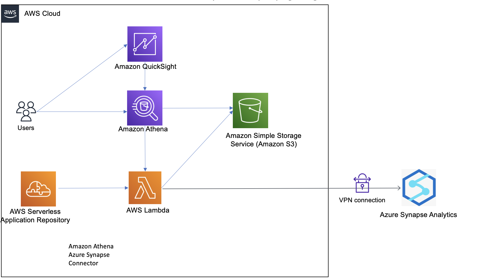
In order to explain this architecture, let’s walk through a sample use case of analyzing fitness data of users. Our sample dataset contains users’ fitness information like age, height, and weight, and daily run stats like miles, calories, average heart rate, and average speed, along with hours of sleep.
We run queries on this dataset to derive insights using visualizations in QuickSight. With QuickSight, you can create trends of daily miles run, keep track of the average heart rate over a period of time, and detect anomalies, if any. You can also track your daily sleep patterns and compare how rest impacts your daily activities. The out-of-the-box insights feature gives vital weekly insights that can help you be on top of your fitness goals. The following screenshot shows sample rows of our dataset stored in Azure Synapse.
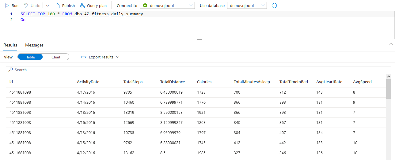
Prerequisites
Make sure you have the following prerequisites:
- An AWS account set up with QuickSight enabled. If you don’t have a QuickSight account, you can sign up for one. You can access the QuickSight free trial as part of the AWS Free Tier option.
- An Azure account with data pre-loaded in Synapse. We use a sample fitness dataset in this post. We used a data generator to generate this data.
- A virtual private connection (VPN) between AWS and Azure.
Note that the AWS resources for the steps in this post need to be in the same Region.
Configure a Lambda connector
To configure your Lambda connector, complete the following steps:
- Load the data.
In the Azure account, the sample data for fitness devices is stored and accessed in an Azure Synapse Analytics workspace using a dedicated SQL pool table. The firewall settings for Synapse should allow for access to a VPC through a VPN. You can use your data or tables that you need to connect QuickSight to in this step.

- On the Amazon S3 console, create a spillover bucket and note the name to use in a later step.
This bucket is used for storing the spillover data for the Synapse connector.
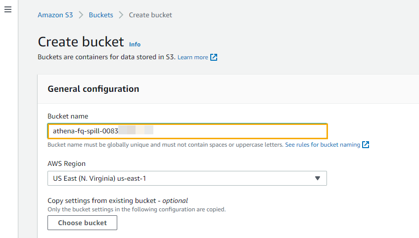
- On the AWS Serverless Application Repository console, choose Available applications in the navigation pane.
- On the Public applications tab, search for
synapseand choose AthenaSynapseConnector with the AWS verified author tag.
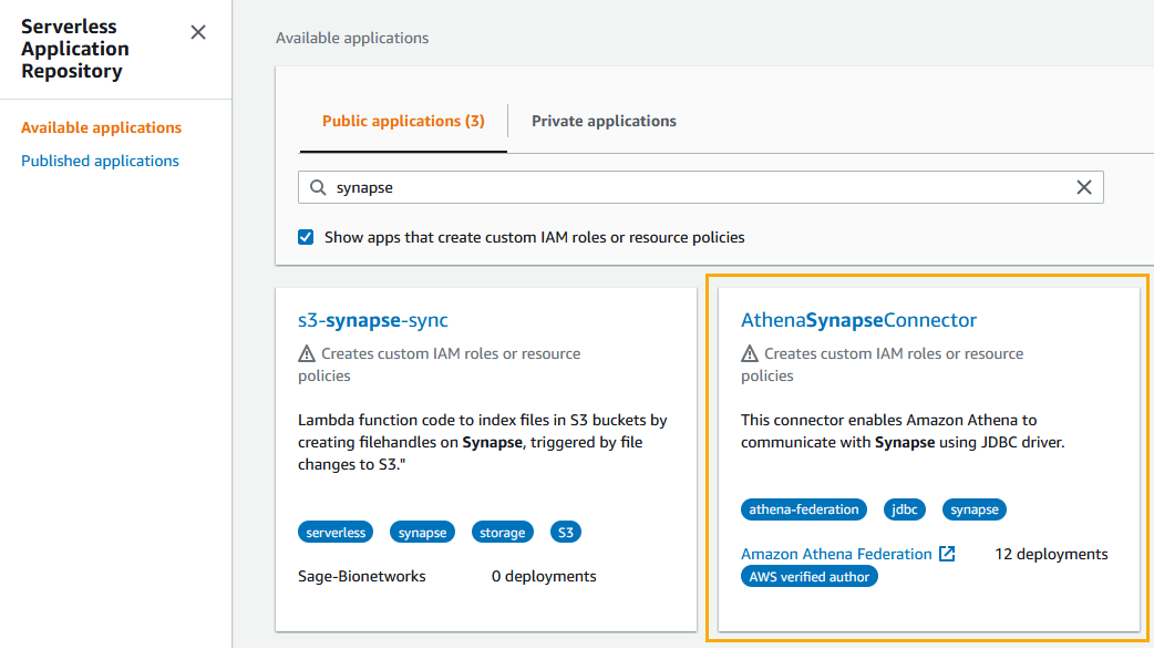
- Create the Lambda function with the following configuration:
- For Name, enter
AthenaSynapseConnector. - For SecretNamePrefix, enter
AthenaJdbcFederation. - For SpillBucket, enter the name of the S3 bucket you created.
- For DefaultConnectionString, enter the JDBC connection string from the Azure SQL pool connection strings property.
- For LambdaFunctionName, enter a function name.
- For SecurityGroupIds and SubnetIds, enter the security group and subnet for your VPC (this is needed for the template to run successfully).
- Leave the remaining values as their default.
- For Name, enter
- Choose Deploy.
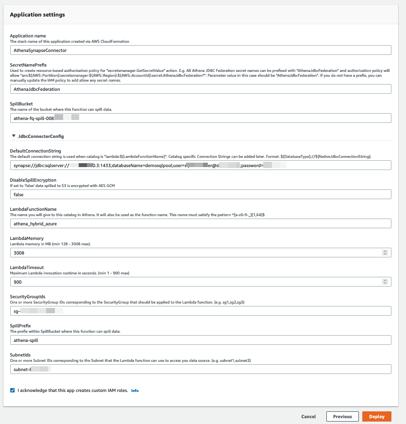
- After the function is deployed successfully, navigate to the
athena\_hybrid\_azurefunction. - On the Configurations tab, choose Environment variables in the navigation pane.
- Add the key
azure\_synapse\_demo\_connection\_stringwith the same value as the default key (the JDBC connection string from the Azure SQL pool connection strings property).
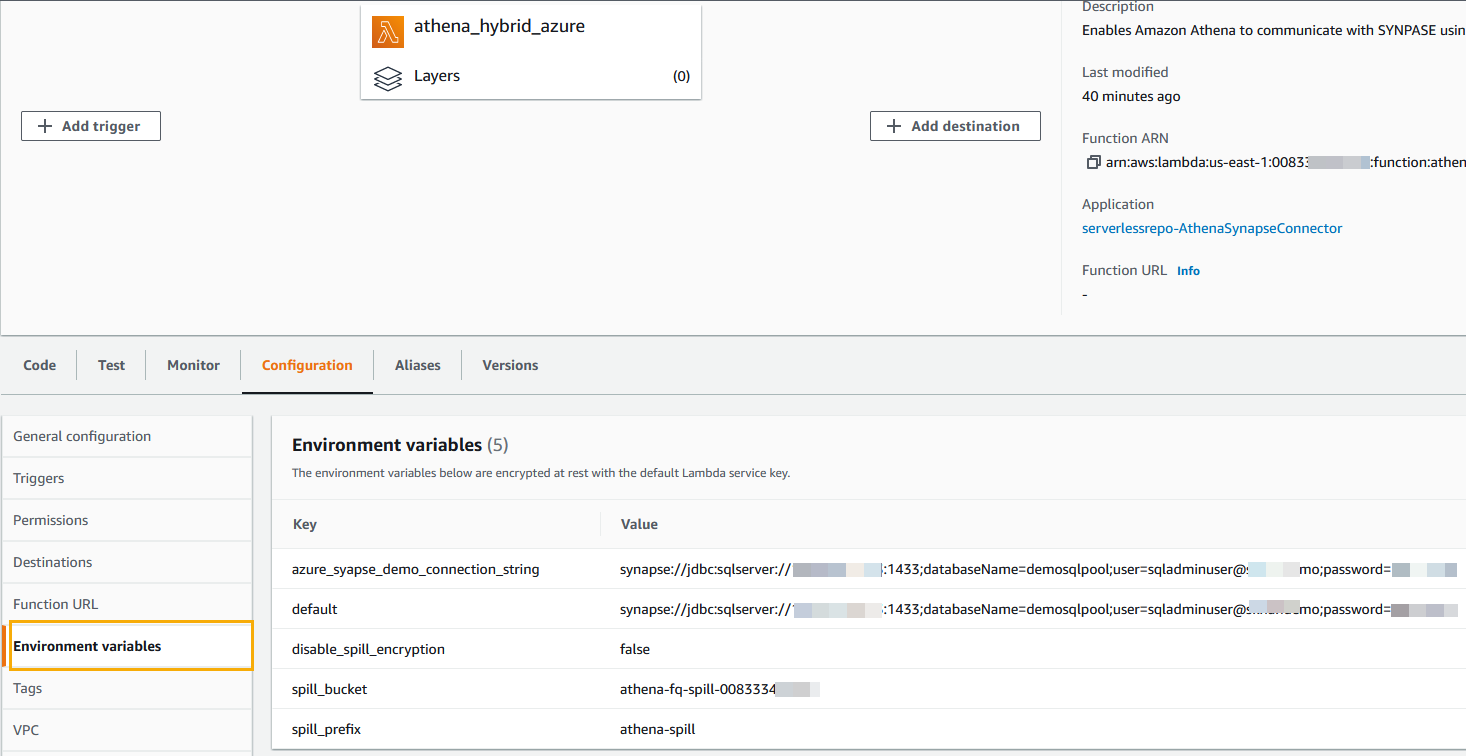
For this post, we removed the VPC configuration. - Choose VPC in the navigation pane and choose None to remove the VPC configuration.
Now you’re ready to configure the data source. - On the Athena console, choose Data sources in the navigation pane.
- Choose Create data source.
- Choose Microsoft Azure Synapse as your data source.
- Choose Next.
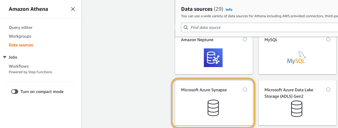
- Create a data source with the following parameters:
- For Data source name, enter
azure\_synapse\_demo. - For Connection details, choose the Lambda function
athena\_hybrid\_azure.
- For Data source name, enter
- Choose Next.

Create a dataset on QuickSight to read the data from Azure Synapse
Now that the configuration on the Athena side is complete, let’s configure QuickSight.
- On the QuickSight console, on the user name menu, choose Manage QuickSight.

- Choose Security & permissions in the navigation pane.
- Under QuickSight access to AWS services, choose Manage.

- Choose Amazon Athena and in the pop-up permissions box, choose Next.

- On the S3 Bucket tab, select the spill bucket you created earlier.
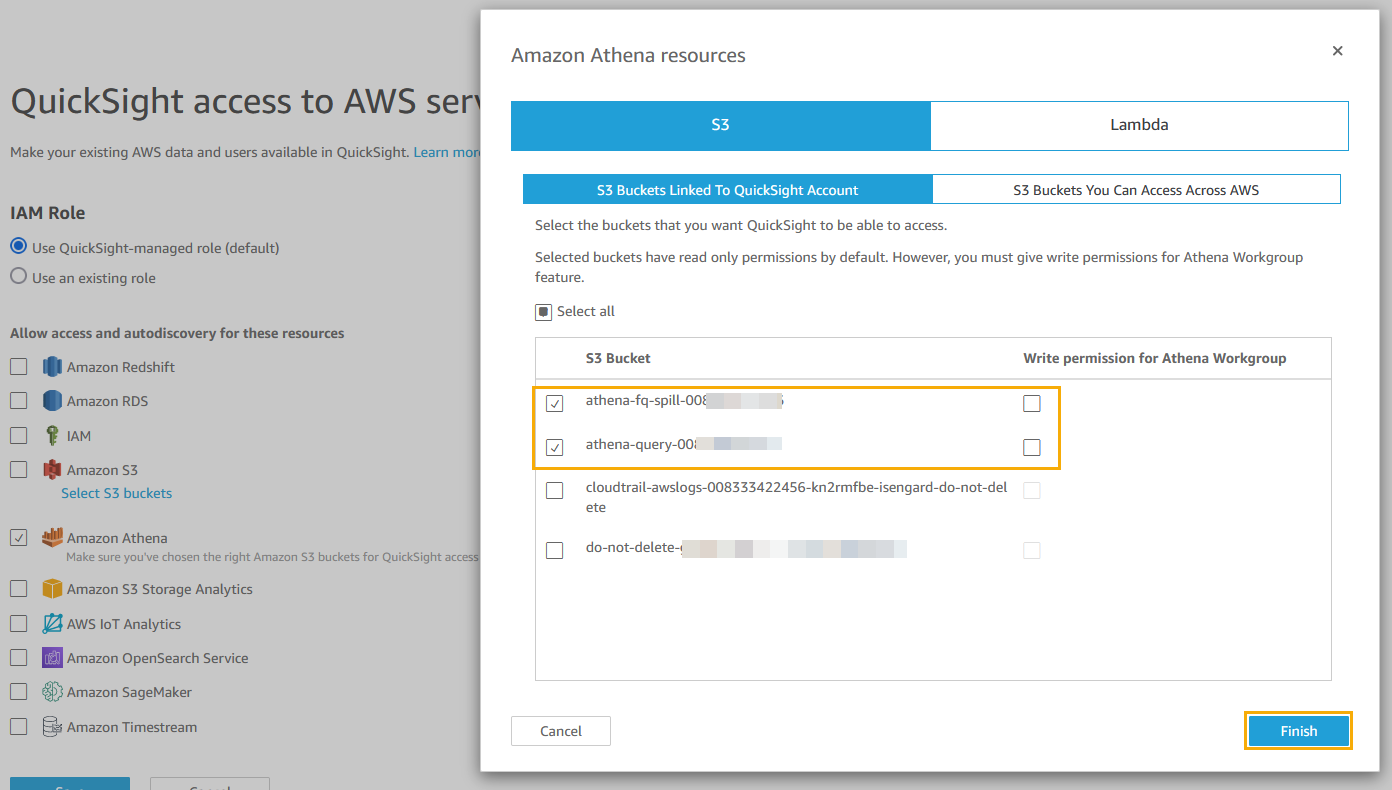
- On the Lambda tab, select the
athena\_hybrid\_azurefunction. - Choose Finish.

- If the QuickSight access to AWS services window appears, choose Save.

- Choose the QuickSight icon on the top left and choose New dataset.

- Choose Athena as the data source.
- For Data source name, enter a name.
- Check the Athena workgroup settings where the Athena data source was created.
- Choose Create data source.

- Choose the catalog
azure\_synapse\_demoand the databasedbo. - Choose Edit/Preview data.
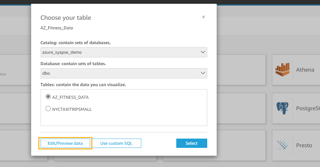
- Change the query mode to SPICE.
- Choose Publish & Visualize.

- Create an analysis in QuickSight.
- Publish a QuickSight dashboard.
If you’re new to QuickSight or looking to build stunning dashboards, this workshop provides step-by-step instructions to grow your dashboard building skills from basic to advanced level. The following screenshot is an example dashboard to give you some inspiration.

Clean up
To avoid ongoing charges, complete the following steps:
- Delete the S3 bucket created for the Athena spill data.
- Delete the Athena data source.
- On the AWS CloudFormation console, select the stack you created for
AthenaSynapseConnectorand choose Delete.
This will delete the created resources, such as the Lambda function. Check the stack’s Events tab to track the progress of the deletion, and wait for the stack status to change to DELETE\_COMPLETE. - Delete the QuickSight datasets.
- Delete the QuickSight analysis.
- Delete your QuickSight subscription and close the account.
Conclusion
In this post, we showed you how to overcome the challenges of connecting to and analyzing data in other clouds by using AWS analytics services to connect to Azure Synapse Analytics with Athena Federated Query and QuickSight. We also showed you how to visualize and derive insights from the fitness data using QuickSight. With QuickSight and Athena Federated Query, organizations can now access additional data sources beyond those already supported natively by QuickSight. If you have data in sources other than Amazon S3, you can use Athena Federated Query to analyze the data in place or build pipelines that extract and store data in Amazon S3.
For more information and resources for QuickSight and Athena, visit Analytics on AWS.
About the authors
 Harish Rajagopalan is a Senior Solutions Architect at Amazon Web Services. Harish works with enterprise customers and helps them with their cloud journey.
 Salim Khan is a Specialist Solutions Architect for Amazon QuickSight. Salim has over 16 years of experience implementing enterprise business intelligence (BI) solutions. Prior to AWS, Salim worked as a BI consultant catering to industry verticals like Automotive, Healthcare, Entertainment, Consumer, Publishing and Financial Services. He has delivered business intelligence, data warehousing, data integration and master data management solutions across enterprises.
 Sriram Vasantha is a Senior Solutions Architect at AWS in Central US helping customers innovate on the cloud. Sriram focuses on application and data modernization, DevSecOps, and digital transformation. In his spare time, Sriram enjoys playing different musical instruments like Piano, Organ, and Guitar.
 Adarsha Nagappasetty is a Senior Solutions Architect at Amazon Web Services. Adarsha works with enterprise customers in Central US and helps them with their cloud journey. In his spare time, Adarsha enjoys spending time outdoors with his family!
Amazon Athena now enables data analysts and data engineers to enjoy the easy-to-use, interactive, serverless experience of Athena with Apache Spark in addition to SQL. You can now use the expressive power of Python and build interactive Apache Spark applications using a simplified notebook experience on the Athena console or through Athena APIs. For interactive […]
AWS Glue is a serverless data integration service that makes it easy to discover, prepare, and combine data for analytics, machine learning (ML), and application development. In AWS Glue, you can use Apache Spark, an open-source, distributed processing system for your data integration tasks and big data workloads. Apache Spark utilizes in-memory caching and optimized […]
Today’s global, data-driven organizations treat data as an asset and use it across different lines of business (LOBs) to drive timely insights and better business decisions. Amazon Redshift data sharing allows you to securely share live, transactionally consistent data in one Amazon Redshift data warehouse with another Amazon Redshift data warehouse within the same AWS […]
It only takes one groundbreaking invention—one iconic idea that solves a widespread pain point for customers—to create or transform an industry forever. From the invention of the telegraph, to the discovery of GPS, to the earliest cloud computing services, history is filled with examples of these “eureka” moments that continue to have long-lasting impacts on […]
We recently announced the preview release of Amazon OpenSearch Serverless, a new serverless option for Amazon OpenSearch Service, which makes it easy for you to run large-scale search and analytics workloads without having to configure, manage, or scale OpenSearch clusters. It automatically provisions and scales the underlying resources to deliver fast data ingestion and query […]
Amazon QuickSight Q uses machine learning (ML) to enable any user to ask questions about business data in natural language and receive accurate answers with relevant visualizations in seconds. Today, Amazon QuickSight announces support for two new question types that simplify and scale complex analytical tasks using natural language: “forecast” and “why.” In this post, […]
Amazon Redshift is the fastest, most widely used, fully managed, petabyte-scale cloud data warehouse. Tens of thousands of customers use Amazon Redshift to process exabytes of data every day to power their analytics workloads. Data engineers, data analysts, and data scientists want to use this data to power analytics workloads such as business intelligence (BI), […]
Amazon Redshift is a fast, fully managed, petabyte-scale cloud data warehouse. You have the flexibility to choose from provisioned and serverless compute modes. You can start loading and querying large datasets conveniently in Amazon Redshift using Amazon Redshift Query Editor v2, a web-based SQL client application. Query Editor v2 empowers your technical and business teams […]
Calculation at the right granularity always needs to be handled carefully when performing data analytics. Especially when data is generated through joining across multiple tables, the denormalization of datasets can add a lot of complications to make accurate calculations challenging. Amazon QuickSight recently launched a new functionality called level-aware calculations (LAC), which enables you to […]
AWS SDK for pandas is an open-source library that extends the popular Python pandas library, enabling you to connect to AWS data and analytics services using pandas data frames. We’ve seen customers use the library in combination with pandas for both data engineering and AI workloads. Although pandas data frames are simple to use, they […]
AWS Glue is a serverless data integration service that makes it simple to discover, prepare, move, and integrate data from multiple sources for analytics, machine learning (ML), and application development. Today, AWS Glue processes customer jobs using either Apache Spark’s distributed processing engine for large workloads or Python’s single-node processing engine for smaller workloads. Customers […]
Amazon OpenSearch Service makes it easy for you to perform interactive log analytics, real-time application monitoring, website search, and more. OpenSearch is an open-source, distributed search and analytics suite comprising OpenSearch, a distributed search and analytics engine, and OpenSearch Dashboards, a UI and visualization tool. When you use Amazon OpenSearch Service, you configure a set […]
We’re excited to announce the launch of small multiples in Amazon QuickSight at AWS re:Invent 2022! Small multiples is one of the most powerful data visualization features when it comes to comparative analysis. Previously, you had to either use a filter or create multiple visuals side by side to analyze multiples slices of the same […]
We are excited to announce the launch of text boxes in Amazon QuickSight. Now you can add text for common use cases, including but not limited to titles, subtitles, annotations, adding additional information for KPIs etc has been simplified than ever before with the new text box. You can reposition, resize, and make your text […]
Amazon QuickSight is a serverless, cloud-based business intelligence (BI) service that brings data insights to your teams and end-users through machine learning (ML)-powered dashboards and data visualizations that can be accessed via QuickSight or embedded in apps and portals that your users access. Line charts in QuickSight have undergone a major overhaul this year, starting […]
This is a guest post co-written with Siva Bangaru and Leon Liu from ADP. ADP helps organizations of all types and sizes by providing human capital management (HCM) solutions that unite HR, payroll, talent, time, tax, and benefits administration. ADP is a leader in business outsourcing services, analytics, and compliance expertise. ADP’s unmatched experience, deep […]
Apache Hudi is an open-source transactional data lake framework that greatly simplifies incremental data processing and data pipeline development. It does this by bringing core warehouse and database functionality directly to a data lake on Amazon Simple Storage Service (Amazon S3) or Apache HDFS. Hudi provides table management, instantaneous views, efficient upserts/deletes, advanced indexes, streaming […]
Amazon Redshift Serverless lets you avoid managing infrastructure while only paying for what you use. Etleap provides data integration software that is natively built on AWS. It’s an AWS Advanced Technology Partner with the AWS Data & Analytics Competency and Amazon Redshift Service Ready designation. In this post, we share how you can minimize the […]
Amazon QuickSight is a fully-managed, cloud-native business intelligence (BI) service that makes it easy to connect to your data, create interactive dashboards, and share these with tens of thousands of users, either within the QuickSight interface or embedded in software as a service (SaaS) applications or web portals. With QuickSight providing insights to power daily […]
The Amazon Alexa Audio Data & Insights (AUDI) team strives to make business intelligence (BI) accessible for engineers across Amazon Alexa Audio. Amazon Alexa Audio helps you stay entertained with your favorite music, podcasts, books, and radio from providers such as Amazon Music, Spotify, and iHeart Radio. The AUDI team manages dashboards and reports to […]
Amazon QuickSight is a fully managed, cloud-native business intelligence (BI) service that makes it easy to connect to your data, create interactive dashboards, and share these with tens of thousands of users, either within the QuickSight interface, or embedded in software as a service (SaaS) applications or web portals. We’re excited to announce the availability […]
This is a guest post co-written with Ankit Jhalaria from GoDaddy. GoDaddy is empowering everyday entrepreneurs by providing all the help and tools to succeed online. With more than 20 million customers worldwide, GoDaddy is the place people come to name their idea, build a professional website, attract customers, and manage their work. GoDaddy is […]
Organizations are placing a high priority on data integration, especially to support analytics, machine learning (ML), business intelligence (BI), and application development initiatives. Data is growing exponentially and is generated by increasingly diverse data sources. Data integration becomes challenging when processing data at scale and the inherent heavy lifting associated with infrastructure required to manage […]
AWS Controllers for Kubernetes (ACK) was announced in August, 2020, and now supports 14 AWS service controllers as generally available with an additional 12 in preview. The vision behind this initiative was simple: allow Kubernetes users to use the Kubernetes API to manage the lifecycle of AWS resources such as Amazon Simple Storage Service (Amazon […]
For data lake customers who need to discover petabytes of data, AWS Glue crawlers are a popular way to scan data in the background, so you can focus on using the data to make better intelligent decisions. You may also have data in data warehouses such as Snowflake and want the ability to discover the […]
ENGIE—one of the largest utility providers in France and a global player in the zero-carbon energy transition—produces, transports, and deals in electricity, gas, and energy services. With 160,000 employees worldwide, ENGIE is a decentralized organization and operates 25 business units with a high level of delegation and empowerment. ENGIE’s decentralized global customer base had accumulated […]
We are delighted to announce the latest version of the Data Analytics Lens, an AWS Well-Architected whitepaper. AWS Well-Architected provides a consistent approach to evaluate architectures and implement scalable designs. The AWS Well-Architected Framework is based on six pillars—operational excellence, security, reliability, performance efficiency, cost optimization, and sustainability. With the framework, cloud architects, system architects, engineers, and developers can build secure, high-performance, resilient, and efficient infrastructure for their applications and workloads.
Amazon Redshift is a fully managed, petabyte-scale data warehouse service in the cloud. You can start with just a few hundred gigabytes of data and scale to a petabyte or more. Today, tens of thousands of AWS customers—from Fortune 500 companies, startups, and everything in between—use Amazon Redshift to run mission-critical business intelligence (BI) dashboards, […]
Amazon EMR on Amazon EKS is a deployment option for Amazon EMR that allows organizations to run Apache Spark on Amazon Elastic Kubernetes Service (Amazon EKS). With EMR on EKS, the Spark jobs run on the Amazon EMR runtime for Apache Spark. This increases the performance of your Spark jobs so that they run faster […]
Fulfillment by Amazon (FBA) was launched in 2006, allowing businesses to outsource shipping to Amazon. With this fulfillment option, Amazon stores, picks, packs, ships, and delivers the products to customer as well as handling the customer service and returns for those orders. Within Seller Central, a website where sellers can monitor their Amazon sales activity, […]
AWS re:Invent is a learning conference hosted by AWS for the global cloud computing community. This year’s re:Invent will be held in Las Vegas, Nevada, from November 28 to December 2. AWS Glue is a serverless data integration service that makes it easier for analytics users to discover, prepare, move, and integrate data from multiple […]
Mark your calendars for November 28 through December 2, 2022 to attend AWS re:Invent in Las Vegas – a learning conference hosted by AWS for the global cloud computing community. To maximize the value of your data, you need to act upon it in real time, instead of waiting for hours, days, or week. AWS […]
In this post, we take the data mesh design discussed in Design a data mesh architecture using AWS Lake Formation and AWS Glue, and demonstrate how to initialize data domain accounts to enable managed sharing; we also go through how we can use an event-driven approach to automate processes between the central governance account and […]
Data engineers and data scientists are dependent on distributed data processing infrastructure like Amazon EMR to perform data processing and advanced analytics jobs on large volumes of data. In most mid-size and enterprise organizations, cloud operations teams own procuring, provisioning, and maintaining the IT infrastructures, and their objectives and best practices differ from the data […]
This is a guest blog post co-written with Addison Higley and Ramzi Yassine from Hudl. Hudl Agile Sports Technologies, Inc. is a Lincoln, Nebraska based company that provides tools for coaches and athletes to review game footage and improve individual and team play. Its initial product line served college and professional American football teams. Today, […]
SOCAR is the leading Korean mobility company with strong competitiveness in car-sharing. SOCAR has become a comprehensive mobility platform in collaboration with Nine2One, an e-bike sharing service, and Modu Company, an online parking platform. Backed by advanced technology and data, SOCAR solves mobility-related social problems, such as parking difficulties and traffic congestion, and changes the […]
Amazon Kinesis Data Analytics is a fully managed service for Apache Flink that reduces the complexity of building, managing, and integrating Apache Flink applications with other AWS services. Apache Flink is an open-source framework and engine for stateful processing of data streams. It’s highly available and scalable, delivering high throughput and low latency for the […]
VPC Flow Logs is an AWS feature that captures information about the network traffic flows going to and from network interfaces in Amazon Virtual Private Cloud (Amazon VPC). Visibility to the network traffic flows of your application can help you troubleshoot connectivity issues, architect your application and network for improved performance, and improve security of […]
This post was co-written with Daniel Gu and Yolanda Wang, from Kyligence. Today, more than ever, organizations realize that modern business runs on data—almost all our interactions with business are based on data, and organizations must use analytics to understand, plan, and improve their operations. That is where Online Analytical Processing (OLAP) comes in. OLAP […]
Amazon OpenSearch Service is fully open-source search and analytics engine that securely unlocks real-time search, monitoring, and analysis of business and operational data for use cases like application monitoring, log analytics, observability, and website search. But what if you have personal identifiable information (PII) data in your log data? How do you control and audit […]
Amazon Athena is an interactive query service that makes it easy to analyze data in Amazon Simple Storage Service (Amazon S3) using standard SQL. Athena is serverless, so there is no infrastructure to manage, and you pay only for the queries that you run on datasets at petabyte scale. You can use Athena to query […]
AWS re:Invent is a learning conference hosted by AWS for the global cloud computing community. This year’s re:Invent will be held in Las Vegas, Nevada, from November 28 to December 2. Amazon QuickSight is the most popular cloud-native serverless BI service. This post walks you through the details of all QuickSight-related sessions and activities to […]
The California State University Chancellor’s Office (CSUCO) sits at the center of America’s most significant and diverse 4-year universities. The California State University (CSU) serves approximately 477,000 students and employs more than 55,000 staff and faculty members across 23 universities and 7 off-campus centers. The CSU provides students with opportunities to develop intellectually and personally, […]
In the first post in our series , we discussed setting up a microservice observability architecture and application troubleshooting steps using log and trace correlation with Amazon OpenSearch Service. In this post, we discuss using PPL to create visualizations in operational panels, and creating a simple incident report using notebooks. To try out the solution […]
This is a guest post by Mehdi Bendriss, Mohamad Shaker, and Arvid Reiche from Scout24. At Scout24 SE, we love data pipelines, with over 700 pipelines running daily in production, spread across over 100 AWS accounts. As we democratize data and our data platform tooling, each team can create, maintain, and run their own data pipelines […]
Join the global cloud community at AWS re:Invent this year to meet, get inspired, and rethink what’s possible! Reserved seating is available for registered attendees to secure seats in the sessions of their choice. You can reserve a seat in your favorite sessions by signing in to the attendee portal and navigating to Event > Sessions. For those who can’t […]
Modern enterprises are increasingly adopting microservice architectures and moving away from monolithic structures. Although microservices provide agility in development and scalability, and encourage use of polyglot systems, they also add complexity. Troubleshooting distributed services is hard because the application behavioral data is distributed across multiple machines. Therefore, in order to have deep insights to troubleshoot […]
Organizations are adopting Apache Kafka and Amazon Managed Streaming for Apache Kafka (Amazon MSK) to capture and analyze data in real-time. Amazon MSK allows you to build and run production applications on Apache Kafka without needing Kafka infrastructure management expertise or having to deal with the complex overheads associated with running Apache Kafka on your […]
Amazon QuickSight is a fully managed, cloud-native business intelligence (BI) service. If you plan to deploy enterprise-grade QuickSight dashboards, measuring user adoption and usage patterns is an important ingredient for the success of your BI investment. For example, knowing the usage patterns like geo location, department, and job role can help you fine-tune your dashboards […]
Amazon Redshift Query Editor V2.0 is a web-based analyst workbench that you can use to author and run queries on your Amazon Redshift data warehouse. You can visualize query results with charts, and explore, share, and collaborate on data with your teams in SQL through a common interface. With SQL Notebooks, Amazon Redshift Query Editor […]
This post is co-written with Darren Demicoli from The Mill Adventure. The Mill Adventure is an iGaming industry enabler offering customizable turnkey solutions to B2B partners and custom branding enablement for its B2C partners. They provide a complete gaming platform, including licenses and operations, for rapid deployment and success in iGaming, and are committed to […]
In the first post of this series, we discussed the need of a metadata management solution for organizations. We used DataHub as an open-source metadata platform for metadata management and deployed it using AWS managed services with the AWS Cloud Development Kit (AWS CDK). In this post, we focus on how to populate technical metadata […]
Many organizations are establishing enterprise data warehouses, data lakes, or a modern data architecture on AWS to build data-driven products. As the organization grows, the number of publishers and subscribers to data and the volume of data keeps increasing. Additionally, different varieties of datasets are introduced (structured, semistructured, and unstructured). This can lead to metadata […]
This post is co-written with Dr. Quan Hoang Nguyen, CTO at Fantom Foundation. Here at Fantom Foundation (Fantom), we have developed a high performance, highly scalable, and secure smart contract platform. It’s designed to overcome limitations of the previous generation of blockchain platforms. The Fantom platform is permissionless, decentralized, and open source. The majority of […]
In this post, we show how to use MSK Connect for MirrorMaker 2 deployment with AWS Identity and Access Management (IAM) authentication. We create an MSK Connect custom plugin and IAM role, and then replicate the data between two existing Amazon Managed Streaming for Apache Kafka (Amazon MSK) clusters. The goal is to have replication […]
As the industry grows with more data volume, big data analytics is becoming a common requirement in data analytics and machine learning (ML) use cases. Data comes from many different sources in structured, semi-structured, and unstructured formats. For semi-structured data, one of the most common lightweight file formats is JSON. However, due to the complex […]
Amazon Redshift Serverless makes it simple to run and scale analytics without having to manage the instance type, instance size, lifecycle management, pausing, resuming, and so on. It automatically provisions and intelligently scales data warehouse compute capacity to deliver fast performance for even the most demanding and unpredictable workloads, and you pay only for what […]
In September 2017, during the annual Splunk.conf, Splunk and AWS jointly announced Amazon Kinesis Data Firehose integration to support Splunk Enterprise and Splunk Cloud as a delivery destination. This native integration between Splunk Enterprise, Splunk Cloud, and Kinesis Data Firehose is designed to make AWS data ingestion setup seamless, while offering a secure and fault-tolerant […]
You can use the Amazon EMR Steps API to submit Apache Hive, Apache Spark, and others types of applications to an EMR cluster. You can invoke the Steps API using Apache Airflow, AWS Steps Functions, the AWS Command Line Interface (AWS CLI), all the AWS SDKs, and the AWS Management Console. Jobs submitted with the […]
Many organizations build data lakes on Amazon Simple Storage Service (Amazon S3) using a modern architecture for a scalable and cost-effective solution. Open-source storage formats like Parquet and Avro are commonly used, and data is stored in these formats as immutable files. As the data lake is expanded to additional use cases, there are still […]
AWS Glue includes crawlers, a capability that make discovering datasets simpler by scanning data in Amazon Simple Storage Service (Amazon S3) and relational databases, extracting their schema, and automatically populating the AWS Glue Data Catalog, which keeps the metadata current. This reduces the time to insight by making newly ingested data quickly available for analysis […]
AWS Glue now offers integration with Git, an open-source version control system widely used across the developer community. Thanks to this integration, you can incorporate your existing DevOps practices on AWS Glue jobs. AWS Glue is a serverless data integration service that helps you create jobs based on Apache Spark or Python to perform extract, […]
Customers tell us they want to have stronger performance and lower costs for their data analytics applications and workloads. Customers also want to use AWS as a platform that hosts managed versions of their favorite open-source projects, which will frequently adopt the latest features from the open-source communities. With Amazon Athena engine version 3, we […]
Today, many companies are building real-time applications to improve their customer experience and get immediate insights from their data before it loses its value. As the result, companies have been facing increasing demand to provide data streaming services such as Apache Kafka for developers. To meet this demand, companies typically start with a small- or […]
In modern data architectures, it’s common to store data in multiple data sources. However, organizations embracing this approach still need insights from their data and require technologies that help them break down data silos. Amazon Athena is an interactive query service that makes it easy to analyze structured, unstructured, and semi-structured data stored in Amazon […]
To build a data lake on AWS, a common data ingestion pattern is to use AWS Glue jobs to perform extract, transform, and load (ETL) data from relational databases to Amazon Simple Storage Service (Amazon S3). A project often involves extracting hundreds of tables from source databases to the data lake raw layer. And for […]
In today’s world with technology modernization, the need for near-real-time streaming use cases has increased exponentially. Many customers are continuously consuming data from different sources, including databases, applications, IoT devices, and sensors. Organizations may need to ingest that streaming data into data lakes built on Amazon Simple Storage Service (Amazon S3). You may also need […]
Stream data processing allows you to act on data in real time. Real-time data analytics can help you have on-time and optimized responses while improving overall customer experience. Apache Flink is a distributed computation framework that allows for stateful real-time data processing. It provides a single set of APIs for building batch and streaming jobs, […]
Amazon QuickSight has launched a new user interface for dataset management. Previously, the dataset management experience was a popup dialog modal with limited space, and all functionality was displayed in this one small modal. The new dataset management experience replaces the existing popup dialog with a full-page experience, providing a clearer breakdown of a dataset’s […]
Amazon Redshift is a fast, scalable, secure, and fully managed cloud data warehouse that makes it simple and cost-effective to analyze all of your data using standard SQL. Tens of thousands of customers today rely on Amazon Redshift to analyze exabytes of data and run complex analytical queries, making it the most widely used cloud […]
This blog post was co-authored with Federico Piccinini. The data landscape has been changing in recent years: there is a proliferation of entities producing and consuming large quantities of data within companies, and for most of them defining a proper data strategy has become of fundamental importance. A modern data strategy gives you a comprehensive […]
AWS Glue is a serverless data integration service that makes it easy to discover, prepare, and combine data for analytics, machine learning (ML), and application development. It’s serverless, so there’s no infrastructure to set up or manage. This post provides a step-by-step guide to build a continuous integration and continuous delivery (CI/CD) pipeline using AWS […]
Data lakes on Amazon Simple Storage Service (Amazon S3) have become the default repository for all enterprise data and serve as a common choice for a large number of users querying from a variety of analytics and machine learning (ML) tools. Oftentimes you want to ingest data continuously into the data lake from multiple sources […]
Amazon OpenSearch Service is a fully managed service that you can use to deploy and operate OpenSearch and legacy Elasticsearch clusters, cost-effectively, at scale in the AWS Cloud. The service makes it easy for you to perform interactive log analytics, real-time application monitoring, website search, and more by offering the latest versions of OpenSearch, support […]
This post is co-written by Martin Zoellner, Thomas Ehrlich and Veronika Bogusch from BMW Group. BMW Group and AWS announced a comprehensive strategic collaboration in 2020. The goal of the collaboration is to further accelerate BMW Group’s pace of innovation by placing data and analytics at the center of its decision-making. A key element of […]
Amazon QuickSight users now can add bookmarks in dashboards to save customized dashboard preferences into a list of bookmarks for easy one-click access to specific views of the dashboard without having to manually make multiple filter and parameter changes every time. Combined with the “Share this view” functionality, you can also now share your bookmark […]
A data lake is a centralized repository that allows you to store all your structured and unstructured data at any scale. You can keep your data as is in your object store or file-based storage without having to first structure the data. Additionally, you can run different types of analytics against your loosely formatted data […]
Nowadays many customers are following a multi-cloud strategy. They might choose to use various cloud-managed services, such as Amazon Relational Database Service (Amazon RDS) for SQL Server and Azure SQL Managed Instances, to perform data analytics tasks, but still use traditional extract, transform, and load (ETL) tools to integrate and process the data. However, traditional ETL tools may […]
There are several infrastructure as code (IaC) frameworks available today, to help you define your infrastructure, such as the AWS Cloud Development Kit (AWS CDK) or Terraform by HashiCorp. Terraform, an AWS Partner Network (APN) Advanced Technology Partner and member of the AWS DevOps Competency, is an IaC tool similar to AWS CloudFormation that allows […]
If you are currently running Amazon EMR 5.X clusters, consider moving to Amazon EMR 6.X as it includes new features that helps you improve performance and optimize on cost. For instance, Apache Hive is two times faster with LLAP on Amazon EMR 6.X, and Spark 3 reduces costs by 40%. Additionally, Amazon EMR 6.x releases […]
IMM (Institutional Money Market) is a mutual fund that invests in highly liquid instruments, cash, and cash equivalents. IMM funds are large financial intermediaries that are crucial to financial stability in the US. Due to its criticality, IMM funds are highly regulated under the security laws, notably Rule 2a-7, Which states that during market stress, […]
Amazon QuickSight Q uses machine learning (ML) and natural language technology to empower you to ask business questions about your data and get answers instantly. You can simply enter your questions (for example, “What is the year-over-year sales trend?”) and get the answer in seconds in the form of a QuickSight visual. Some business questions […]
Many AWS customers use Amazon Elastic Kubernetes Service (Amazon EKS) in order to take advantage of Kubernetes without the burden of managing the Kubernetes control plane. With Kubernetes, you can centrally manage your workloads and offer administrators a multi-tenant environment where they can create, update, scale, and secure workloads using a single API. Kubernetes also […]
Data lakes offer the possibility of sharing diverse types of data with different teams and roles to cover numerous use cases. This is very important in order to implement a data democratization strategy and incentivize the collaboration between lines of business. When a data lake is being designed, one of the most important aspects to […]
This is post is co-authored by Manish Mehra, Anirudh Vohra, Sidrah Sayyad, and Abhishek I S (from ZS), and Parnab Basak (from AWS). The team at ZS collaborated closely with AWS to build a modern, cloud-native data orchestration platform. ZS is a management consulting and technology firm focused on transforming global healthcare and beyond. We […]
Customers migrating from large on-premises Hadoop clusters to Amazon EMR like to reduce their operational costs while running resilient applications. On-premises customers typically use in-elastic, large, fixed-size Hadoop clusters, which incurs high capital expenditure. You can now migrate your mixed workloads to managed scaling Amazon EMR, which saves costs without compromising performance. This solution can […]
In today’s world, organizations are collecting an unprecedented amount of data from all kinds of different data sources, such as transactional data stores, clickstreams, log data, IoT data, and more. This data is often in different formats, such as structured data or unstructured data, and is usually referred to as the three Vs of big […]
Data warehouses and data lakes are key to an enterprise data management strategy. A data lake is a centralized repository that consolidates your data in any format at any scale and makes it available for different kinds of analytics. A data warehouse, on the other hand, has cleansed, enriched, and transformed data that is optimized […]
Enterprise customers are modernizing their data warehouses and data lakes to provide real-time insights, because having the right insights at the right time is crucial for good business outcomes. To enable near-real-time decision-making, data pipelines need to process real-time or near-real-time data. This data is sourced from IoT devices, change data capture (CDC) services like […]
Amazon QuickSight is a fully-managed, cloud-native business intelligence (BI) service that makes it easy to create and deliver insights to everyone in your organization or even with your customers and partners. You can make your data come to life with rich interactive charts and create beautiful dashboards to share with thousands of users, either directly […]
With Amazon EMR, you can use a security configuration to specify settings for encrypting data in transit. When in-transit encryption is configured, you can enable application-specific encryption features, for example: Hadoop HDFS NameNode or DataNode user interfaces use HTTPS Hadoop MapReduce encrypted shuffle uses Transport Layer Security (TLS) Presto nodes internal communication uses SSL/TLS (Amazon […]
Amazon Redshift Serverless makes it easy to run and scale analytics in seconds without the need to setup and manage data warehouse clusters. With Redshift Serverless, users such as data analysts, developers, business professionals, and data scientists can get insights from data by simply loading and querying data in the data warehouse. With Redshift Serverless, […]
In legacy relational database management systems, data is stored in several complex data types, such XML, JSON, BLOB, or CLOB. This data might contain valuable information that is often difficult to transform into insights, so you might be looking for ways to load and use this data in a modern cloud data warehouse such as […]
Amazon QuickSight is a scalable, serverless, embeddable, machine learning (ML)-powered business intelligence (BI) service built for the cloud that supports identity federation in both Standard and Enterprise editions. Organizations are working towards centralizing their identity and access strategy across all of their applications, including on-premises, third-party, and applications on AWS. Many organizations use Ping One […]
Amazon QuickSight is a serverless, cloud-based business intelligence (BI) service that brings data insights to your teams and end-users through machine learning (ML)-powered dashboards and data visualizations, which can be accessed via QuickSight or embedded in apps and portals that your users access. This post shares the top QuickSight features and updates launched in Q2 […]
A data lake is a centralized, curated, and secured repository that stores all your data, both in its original form and prepared for analysis. Setting up and managing data lakes today involves a lot of manual, complicated, and time-consuming tasks. AWS Glue and AWS Lake Formation make it easy to build, secure, and manage data […]
Grafana is a popular open-source analytics platform that you can employ to create, explore, and share your data through flexible dashboards. Its use cases include application and IoT device monitoring, and visualization of operational and business data, among others. You can create your dashboard with your own datasets or publicly available datasets related to your […]
Applications today generate enormous amounts of data. This provides an incredible opportunity for independent software vendors (ISV) to deliver business intelligence (BI) offerings as a part of their application, providing visuals, dashboards, and self-service capabilities to customers. These insights are crucial for data-driven decision-making for end-users of these apps, especially if surfaced in the moments […]
This post is co-written by Kanti Singh, Director of Data & Analytics at Fresenius Medical Care. Fresenius Medical Care is the world’s leading provider of kidney care products and services, and operates more than 2,600 dialysis centers in the US alone. The company provides comprehensive solutions for people living with chronic kidney disease and related […]
This is a guest post co-written by Sergei Dubinin, Oleksandr Ierenkov, Illia Popov and Joel Thompson, from Bridgewater. Bridgewater’s core mission is to understand how the world works by analyzing the drivers of markets and turning that understanding into high-quality portfolios and investment advice for our clients. Within Bridgewater Technology, we strive to make our […]
Amazon Managed Streaming for Apache Kafka (Amazon MSK) runs Apache Kafka clusters for you in the cloud. Although using cloud services means you don’t have to manage racks of servers any more, we take advantage of rack aware features in Apache Kafka to spread risk across AWS Availability Zones and increase availability of Amazon MSK […]
This post is co-written by Kiran Ramineni and Basava Hubli, from Fannie Mae. Amazon Redshift data sharing enables instant, granular, and fast data access across Amazon Redshift clusters without the need to copy or move data around. Data sharing provides live access to data so that users always see the most up-to-date and transactionally consistent […]
Tens of thousands of AWS customers choose Amazon Simple Storage Service (Amazon S3) as their data lake to run big data analytics, interactive queries, high-performance computing, and artificial intelligence (AI) and machine learning (ML) applications to gain business insights from their data. On top of these data lakes, you can use AWS Lake Formation to […]
Amazon Redshift is a fast, fully managed cloud data warehouse that makes it simple and cost-effective to analyze all your data using standard SQL and your existing business intelligence (BI) tools. Amazon Redshift data sharing allows for a secure and easy way to share live data for reading across Amazon Redshift clusters. It allows an […]
Amazon QuickSight is a fully-managed, cloud-native business intelligence (BI) service that makes it easy to create and deliver insights to everyone in your organization. You can make your data come to life with rich interactive charts and create beautiful dashboards to share with thousands of users, either directly within a QuickSight application, or embedded in […]
Interactive Sessions for Jupyter is a new notebook interface in the AWS Glue serverless Spark environment. Starting in seconds and automatically stopping compute when idle, interactive sessions provide an on-demand, highly-scalable, serverless Spark backend to Jupyter notebooks and Jupyter-based IDEs such as Jupyter Lab, Microsoft Visual Studio Code, JetBrains PyCharm, and more. Interactive sessions replace […]
Amazon Redshift is a fully managed, petabyte-scale, massively parallel data warehouse that offers simple operations and high performance. It makes it fast, simple, and cost-effective to analyze all your data using standard SQL and your existing business intelligence (BI) tools. Today, Amazon Redshift has become the most widely used cloud data warehouse. With the significant […]
Apache Hadoop YARN (Yet Another Resource Negotiator) is a cluster resource manager responsible for assigning computational resources (CPU, memory, I/O), and scheduling and monitoring jobs submitted to a Hadoop cluster. This generic framework allows for effective management of cluster resources for distributed data processing frameworks, such as Apache Spark, Apache MapReduce, and Apache Hive. When […]
Amazon Redshift provides resiliency in the event of a single point of failure in a cluster, including automatically detecting and recovering from drive and node failures. The Amazon Redshift relocation feature adds an additional level of availability, and this post is focused on explaining this automatic recovery feature. When the cluster relocation feature is enabled […]
Amazon EMR on EKS is a deployment option that enables you to run Spark workloads on Amazon Elastic Kubernetes Service (Amazon EKS) easily. It allows you to innovate faster with the latest Apache Spark on Kubernetes architecture while benefiting from the performance-optimized Spark runtime powered by Amazon EMR. This deployment option elects Amazon EKS as […]
AWS Glue is the central service of an AWS modern data architecture. It is a serverless data integration service that allows you to discover, prepare, and combine data for analytics and machine learning. AWS Glue offers you a comprehensive range of tools to perform ETL (extract, transform, and load) at the right scale. AWS Glue […]
According to an article in MIT Sloan Management Review, 9 out of 10 companies believe their industry will be digitally disrupted. In order to fuel the digital disruption, companies are eager to gather as much data as possible. Given the importance of this new asset, lawmakers are keen to protect the privacy of individuals and […]
This is a guest post by Kevin Chun, Staff Software Engineer in Core Engineering at NerdWallet. NerdWallet’s mission is to provide clarity for all of life’s financial decisions. This covers a diverse set of topics: from choosing the right credit card, to managing your spending, to finding the best personal loan, to refinancing your mortgage. […]
AWS Glue is a serverless data integration service that makes it simple to discover, prepare, and combine data for analytics, machine learning (ML), and application development. You can use AWS Glue to create, run, and monitor data integration and ETL (extract, transform, and load) pipelines and catalog your assets across multiple data stores. Typically, these […]
This is a guest post by Faye Crompton from Forwood Safety. Forwood provides fatality prevention solutions to organizations across the globe. At Forwood Safety, we have a laser focus on saving lives. Our solutions, which provide full content and proven methodology via verification tools and analytical capabilities, have one purpose: eliminating fatalities in the workplace. […]
Amazon EMR on Amazon EKS enables you to submit Apache Spark jobs on demand on Amazon Elastic Kubernetes Service (Amazon EKS) without provisioning clusters. With EMR on EKS, you can consolidate analytical workloads with your other Kubernetes-based applications on the same Amazon EKS cluster to improve resource utilization and simplify infrastructure management. Kubernetes uses namespaces to provide isolation between […]
AWS Glue streaming extract, transform, and load (ETL) jobs allow you to process and enrich vast amounts of incoming data from systems such as Amazon Kinesis Data Streams, Amazon Managed Streaming for Apache Kafka (Amazon MSK), or any other Apache Kafka cluster. It uses the Spark Structured Streaming framework to perform data processing in near-real […]
Amazon Redshift is a fully managed, petabyte-scale data warehouse service in the cloud. You can start with just a few hundred gigabytes of data and scale to a petabyte or more. Amazon Redshift enables you to use your data to acquire new insights for your business and customers while keeping costs low. Together with price-performance, […]
Amazon Redshift RSQL is a command-line client for interacting with Amazon Redshift clusters and databases. You can connect to an Amazon Redshift cluster, describe database objects, query data, and view query results in various output formats. You can use enhanced control flow commands to replace existing extract, transform, load (ETL) and automation scripts. This post […]
Epos Now provides point of sale and payment solutions to over 40,000 hospitality and retailers across 71 countries. Their mission is to help businesses of all sizes reach their full potential through the power of cloud technology, with solutions that are affordable, efficient, and accessible. Their solutions allow businesses to leverage actionable insights, manage their […]
In the post Data preparation using Amazon Redshift with AWS Glue DataBrew, we saw how to create an AWS Glue DataBrew job using a JDBC connection for Amazon Redshift. In this post, we show you how to create a DataBrew profile job and a recipe job using an Amazon Redshift connection with custom SQL. DataBrew […]
Amazon QuickSight is a cloud-scale business intelligence (BI) service that you can use to deliver easy-to-understand insights to the people you work with, wherever they are. You can build dashboards using combinations of data in the cloud, on premises, in other software as a service (SaaS) apps, and in flat files. Although users can always […]
This is the sixth in a series of posts. We’re excited to share dozens of new features to automate your schema conversion; preserve your investment in existing scripts, reports, and applications; accelerate query performance; and potentially simplify your migrations from legacy data warehouses to Amazon Redshift. Check out all the previous posts in this series: […]
Amazon QuickSight is a fully-managed, cloud-native business intelligence (BI) service that makes it easy to connect to your data, create interactive dashboards, and share these with tens of thousands of users, either within QuickSight itself or embedded in apps and portals. QuickSight Enterprise Edition recently introduced the ability to dynamically allow list the domains where […]
Building a robust data lake is very beneficial because it enables organizations have a holistic view of their business and empowers data-driven decisions. The curated layer of a data lake is able to hydrate multiple homogeneous data products, unlocking limitless capabilities to address current and future requirements. However, some concepts of how data lakes work […]
This post was co-authored by Vadym Dolin, Data Architect at SumUp. In their own words, SumUp is a leading financial technology company, operating across 35 markets on three continents. SumUp helps small businesses be successful by enabling them to accept card payments in-store, in-app, and online, in a simple, secure, and cost-effective way. Today, SumUp […]
Transactional data lake technologies such as Apache Hudi, Delta Lake, Apache Iceberg, and AWS Lake Formation governed tables is evolving rapidly, and gaining great popularity. These technologies simplified the data processing pipeline significantly, and they provided further useful capabilities like upserts, rolling back, and time travel queries. In the first post of this series, we went […]
Amazon Redshift is a fast, fully managed cloud data warehouse that makes it simple and cost-effective to analyze all your data using standard SQL and your existing business intelligence (BI) tools. Many customers look to build their data warehouse on Amazon Redshift, and they have many requirements where they want to convert data from row […]
Spark jobs running on Amazon EMR on EKS generate logs that are very useful in identifying issues with Spark processes and also as a way to see Spark outputs. You can access these logs from a variety of sources. On the Amazon EMR virtual cluster console, you can access logs from the Spark History UI. […]
Amazon Redshift is a fully managed, petabyte-scale data warehouse service in the cloud. You can start with just a few hundred gigabytes of data and scale to a petabyte or more. This enables you to use your data to acquire new insights for your business and customers. As enterprise customers look to build their data […]
Managing data through a central data platform simplifies staffing and training challenges and reduces the costs. However, it can create scaling, ownership, and accountability challenges, because central teams may not understand the specific needs of a data domain, whether it’s because of data types and storage, security, data catalog requirements, or specific technologies needed for […]
Cloud data lakes provides a scalable and low-cost data repository that enables customers to easily store data from a variety of data sources. Data scientists, business analysts, and line of business users leverage data lake to explore, refine, and analyze petabytes of data. AWS Glue is a serverless data integration service that makes it easy […]
Plugsurfing aligns the entire car charging ecosystem—drivers, charging point operators, and carmakers—within a single platform. The over 1 million drivers connected to the Plugsurfing Power Platform benefit from a network of over 300,000 charging points across Europe. Plugsurfing serves charging point operators with a backend cloud software for managing everything from country-specific regulations to providing […]
In this second post of a multi-part series, we share best practices for choosing the optimal Amazon Redshift cluster, data architecture, converting stored procedures, compatible functions and queries widely used for SQL conversions, and recommendations for optimizing the length of data types for table columns. You can check out the first post of this series […]
A data warehouse collects and consolidates data from various sources within your organization. It’s used as a centralized data repository for analytics and business intelligence. When working with on-premises legacy data warehouses, scaling the size of your data warehouse or improving performance can mean purchasing new hardware or adding more powerful hardware. This is often […]
Amazon Redshift has improved the performance of the classic resize feature and increased the flexibility of the cluster snapshot restore operation. You can use the classic resize operation to resize a cluster when you need to change the instance type or transition to a configuration that can’t be supported by elastic resize. This could take […]
Amazon OpenSearch Service is a fully managed service that you can use to deploy and operate OpenSearch clusters cost-effectively at scale in the AWS Cloud. The service makes it easy for you to perform interactive log analytics, real-time application monitoring, website search, and more by offering the latest versions of OpenSearch, support for 19 versions […]
We are excited to announce Embedded Analytics Data Lab (EADL), a no-cost collaborative engagement that helps engineering and development teams cut down time required to launch applications with embedded analytics from Amazon QuickSight in production by providing hands-on guidance and architectural best practices. Embedding rich analytics such as interactive visuals and dashboards directly into applications […]
Amazon Redshift is a fast, fully managed cloud data warehouse database that makes it cost-effective to analyze your data using standard SQL and business intelligence tools. Amazon Redshift allows you to analyze structured and semi-structured data and seamlessly query data lakes and operational databases, using AWS designed hardware and automated machine learning (ML)-based tuning to […]
Amazon Redshift is a fully managed, petabyte-scale data warehouse service in the cloud. With Amazon Redshift, you can analyze all your data to derive holistic insights about your business and your customers. One of the challenges with security is that enterprises want to provide fine-grained access control at the row level for sensitive data. You […]
Amazon Athena now provides you more flexibility to use parameterized queries, and we recommend you use them as the best practice for your Athena queries moving forward so you benefit from the security, reusability, and simplicity they offer. In a previous post, Improve reusability and security using Amazon Athena parameterized queries, we explained how parameterized […]
Amazon Redshift ML makes it easy for SQL users to create, train, and deploy ML models using familiar SQL commands. Redshift ML allows you to use your data in Amazon Redshift with Amazon SageMaker, a fully managed ML service, without requiring you to become an expert in ML. AWS Data Exchange makes it easy to […]
This blog post is co-authored with Erick Leon, Sr. Technical Alliance Manager from Dynatrace. Amazon Kinesis Data Firehose is the easiest way to reliably load streaming data into data lakes, data stores, and analytics services. With just a few clicks, you can create fully-managed delivery streams that auto scale on demand to match the throughput of […]
Social gaming and online sports betting are competitive environments. The game must be able to handle large volumes of unpredictable traffic while simultaneously promising zero downtime. In this domain, user retention is no longer just desirable, it’s critical. William Hill is a global online gambling company based in London, England, and it is the founding […]
Amazon Redshift is a fast, scalable, secure, and fully-managed cloud data warehouse that makes it simple and cost-effective to analyze all of your data using standard SQL. Amazon Redshift has comprehensive security capabilities to satisfy the most demanding requirements. To help you to monitor the database for security and troubleshooting purposes, Amazon Redshift logs information […]
Amazon QuickSight is a fully-managed, cloud-native business intelligence (BI) service that makes it easy to connect to your data, create interactive dashboards, and share these with tens of thousands of users, either within the QuickSight interface or embedded in software as a service (SaaS) applications or web portals. With QuickSight providing insights to power your […]
Amazon Keyspaces (for Apache Cassandra) is a scalable, highly available, and managed Apache Cassandra–compatible database service. With Amazon Keyspaces you don’t have to provision, patch, or manage servers, and you don’t have to install, maintain, or operate software. Amazon Keyspaces is serverless, so you only pay for the resources that you use. You can use […]
As the most widely used cloud data warehouse, Amazon Redshift makes it simple and cost-effective to analyze your data using standard SQL and your existing ETL (extract, transform, and load), business intelligence (BI), and reporting tools. Tens of thousands of customers use Amazon Redshift to analyze exabytes of data per day and power analytics workloads […]
Amazon EMR is a cloud big data platform for running large-scale distributed data processing jobs, interactive SQL queries, and machine learning (ML) applications using open-source analytics frameworks such as Apache Spark, Apache Hive, and Presto. Amazon EMR launches all nodes for a given cluster in the same Amazon Elastic Compute Cloud (Amazon EC2) Availability Zone […]
Amazon EMR is a cloud big data platform for running large-scale distributed data processing jobs, interactive SQL queries, and machine learning (ML) applications using open-source analytics frameworks such as Apache Spark, Apache Hive, and Presto. Apache Iceberg is an open table format for huge analytic datasets. Table formats typically indicate the format and location of […]
Amazon QuickSight is a scalable, serverless, embeddable, machine learning (ML)-powered business intelligence (BI) service built for the cloud that supports identity federation in both Standard and Enterprise editions. Organizations are working towards centralizing their identity and access strategy across all their applications, including on premises, third-party, and applications on AWS. Many organizations use identity providers […]
Modern data architectures encourage the integration of data lakes, data warehouses, and purpose-built data stores, enabling unified governance and easy data movement. With a modern data architecture on AWS, you can store data in a data lake and use a ring of purpose-built data services around the lake, allowing you to make decisions with speed […]
In this post, we discuss how to use AWS Database Migration Service (AWS DMS) native change data capture (CDC) capabilities to stream changes into Amazon Kinesis Data Streams. AWS DMS is a cloud service that makes it easy to migrate relational databases, data warehouses, NoSQL databases, and other types of data stores. You can use […]
Amazon Managed Grafana recently announced a new data source plugin for Amazon Redshift, enabling you to query, visualize, and alert on your Amazon Redshift data from Amazon Managed Grafana workspaces. With the new Amazon Redshift data source, you can now create dashboards and alerts in your Amazon Managed Grafana workspaces to analyze your structured and […]
Nowadays, many customers have built their data lakes as the core of their data analytic systems. In a typical use case of data lakes, many concurrent queries run to retrieve consistent snapshots of business insights by aggregating query results. A large volume of data constantly comes from different data sources into the data lakes. There […]
Most businesses store their critical data in a data lake, where you can bring data from various sources to a centralized storage. The data is processed by specialized big data compute engines, such as Amazon Athena for interactive queries, Amazon EMR for Apache Spark applications, Amazon SageMaker for machine learning, and Amazon QuickSight for data […]
Amazon Redshift is a popular cloud data warehouse that allows you to process exabytes of data across your data warehouse, operational database, and data lake using standard SQL. Amazon Redshift offers different node types like DC2 (dense compute) and RA3, which you can use for your different workloads and use cases. For more information about […]
As the implementation of data lakes and modern data architecture increases, customers’ expectations around its features also increase, which include ACID transaction, UPSERT, time travel, schema evolution, auto compaction, and many more. By default, Amazon Simple Storage Service (Amazon S3) objects are immutable, which means you can’t update records in your data lake because it […]
This is post is co-authored by Jyothin Madari, Madhusudhan Muppagowni and Ayush Srivastava from GE. GE Proficy Manufacturing Data Cloud (MDC), part of the GE Digital’s Manufacturing Execution Systems (MES) suite of solutions, allows GED’s customers to increase the derived value easily and quickly from the MES by reliably bringing enterprise-wide manufacturing data into the […]
Amazon Athena is an interactive query service that makes it easy to analyze data in Amazon Simple Storage Service (Amazon S3) using standard SQL. Athena is serverless, so there is no infrastructure to manage, and you pay only for the queries that you run. In 2019, Athena added support for federated queries to run SQL […]
Security-conscious customers often adopt a Zero Trust security architecture. Zero Trust is a security model centered on the idea that access to data shouldn’t be solely based on network location, but rather require users and systems to prove their identities and trustworthiness and enforce fine-grained identity-based authorization rules before granting access to applications, data, and […]
Data engineers use various Python packages to meet their data processing requirements while building data pipelines with AWS Glue PySpark Jobs. Languages like Python and Scala are commonly used in data pipeline development. Developers can take advantage of their open-source packages or even customize their own to make it easier and faster to perform use […]
Amazon QuickSight is a serverless business intelligence (BI) service used by organizations of any size to make better data-driven decisions. QuickSight dashboards can also be embedded into SaaS apps and web portals to provide interactive dashboards, natural language query or data analysis capabilities to app users seamlessly. The QuickSight Demo Central contains many dashboards, feature showcase […]
Amazon QuickSight was launched in November 2016 as a fast, cloud-powered business analytics service to build visualizations, perform ad hoc analysis, and quickly get business insights from a variety of data sources. In 2018, ML Insights for QuickSight (Enterprise Edition) was announced to add machine learning (ML)-powered forecasting and anomaly detection with a few clicks. […]
Do you want to reduce stockouts at stores? Do you want to improve order delivery timelines? Do you want to provide your customers with accurate product availability, down to the millisecond? A retail operational data lake can help you transform the customer experience by providing deeper insights into a variety of operational aspects of your […]
A lot of the power behind business intelligence (BI) and data visualization tools such as Amazon QuickSight comes from the ability to work interactively with data through a GUI. Report authors create dashboards using GUI-based tools, then in just a few clicks can share the dashboards with business users and decision-makers. This workflow empowers authors […]
Organizations today have continuous incoming data, and analyzing this data in a timely fashion is becoming a common requirement for data analytics and machine learning (ML) use cases. As part of this, you need clean data in order to gain insights that can enable enterprises to get the most out of their data for business […]
Metadata is an integral part of data management and governance. The AWS Glue Data Catalog can provide a uniform repository to store and share metadata. The main purpose of the Data Catalog is to provide a central metadata store where disparate systems can store, discover, and use that metadata to query and process the data. […]
This is a guest post by Dhanraj Gaikwad, Principal Engineer on Dream11 Data Engineering team. Dream11 is the world’s largest fantasy sports platform, with over 120 million users playing fantasy cricket, football, kabaddi, basketball, hockey, volleyball, handball, rugby, futsal, American football, and baseball. Dream11 is the flagship brand of Dream Sports, India’s leading Sports Technology […]
In this post, you will learn how to use Amazon Athena Federated Query to connect a MongoDB database to Amazon QuickSight in order to build dashboards and visualizations. Amazon Athena is a serverless interactive query service, based on Presto, that provides full ANSI SQL support to query a variety of standard data formats, including CSV, […]
AWS Glue has become a popular option for integrating data from disparate data sources due to its ability to integrate large volumes of data using distributed data processing frameworks. Many customers use AWS Glue to build data lakes and data warehouses. Data engineers who prefer to develop data processing pipelines visually using AWS Glue Studio […]
Amazon QuickSight is a scalable, serverless, embeddable, machine learning (ML)-powered business intelligence (BI) service built for the cloud that supports identity federation in both Standard and Enterprise editions. Organizations are working towards centralizing their identity and access strategy across all of their applications, including on-premises, third-party, and applications on AWS. Many organizations use Google Workspace […]
Amazon QuickSight is cloud-native business intelligence (BI) service. QuickSight automatically optimizes queries and execution to help dashboards load quickly, but you can make your dashboard loads even faster and make sure you’re getting the best possible performance by following the tips and tricks outlined in this post. Data flow and execution of QuickSight dashboard loads […]
Amazon Athena is an interactive query service that makes it easy to analyze data in Amazon Simple Storage Service (Amazon S3) using standard SQL. Athena is serverless, so there is no infrastructure to manage, and you pay only for the queries that you run. Amazon Ion is a richly typed, self-describing, hierarchical data serialization format […]
Amazon Redshift is a fully managed, petabyte-scale data warehouse service in the cloud. You can start with just a few hundred gigabytes of data and scale to a petabyte or more. This enables you to use your data to acquire new insights for your business and customers. Over the years, Amazon Redshift has evolved a […]
Enterprises typically host a myriad of business applications for varying data needs. As companies grow, so does the demand for insights from a complete set of business data. Having data from various applications that store data in disparate silos can delay the decision-making process. However, building and maintaining an API integration or a third-party extract, […]
Starting June 30, 2022, Amazon QuickSight is introducing the new look and feel for your dashboards. In this post, we walk through the changes to expect with the new look. The new dashboard experience includes the following improvements: Simplified toolbar Discoverable visual menu Polished controls, menu, and submenus Non-blocking right pane for secondary experiences like […]
Amazon Redshift is the fastest, most widely used, fully managed, and petabyte-scale cloud data warehouse. Tens of thousands of customers use Amazon Redshift to process exabytes of data every day to power their analytics workloads. Amazon Redshift ML, powered by Amazon SageMaker, makes it easy for SQL users such as data analysts, data scientists, and […]
Many of our customers that use Amazon EMR as their big data platform need to integrate with their existing Microsoft Active Directory (AD) for user authentication. This integration requires the Kerberos daemon of Amazon EMR to establish a trusted connection with an AD domain, which involves a lot of moving pieces and can be difficult […]
Amazon Redshift query editor v2 is a web-based SQL client application that you can use to author and run queries on your Amazon Redshift data warehouse. You can visualize query results with charts and collaborate by sharing queries with members of your team. You can use query editor v2 to create databases, schemas, tables, and […]
In the first post of this series, Federate access to your Amazon Redshift cluster with Active Directory Federation Services (AD FS): Part 1, you set up Microsoft Active Directory Federation Services (AD FS) and Security Assertion Markup Language (SAML) based authentication and tested the SAML federation using a web browser. In Part 2, you learned […]
This post was co-written by Rajat Bhardwaj, Senior Technical Account Manager at AWS and Kunal Upadhyay, General Manager at Paytm. Paytm is India’s leading payment platform, pioneering the digital payment era in India with 130 million active users. Paytm operates multiple lines of business, including banking, digital payments, bill recharges, e-wallet, stocks, insurance, lending and […]
Customers with specific needs to run big data compute jobs on an on-premises infrastructure often require a scalable orchestration solution. For large-scale distributed compute clusters, the orchestration of jobs must be scalable to maximize their utilization, while at the same time remain resilient to any failures to prevent blocking the ever-growing influx of data and […]
Email is one of the most important methods for business communication across many organizations. It’s also one of the primary methods for many businesses to communicate with their customers. With the ever-increasing necessity to send emails at scale, monitoring and analysis has become a major challenge. Amazon Simple Email Service (Amazon SES) is a cost-effective, […]
With real-time information about customers, products, and applications in hand, organizations can take action as events happen in their business application. For example, you can prevent financial fraud, deliver personalized offers, and identify and prevent failures before they occur in near real time. Although batch analytics provides abilities to analyze trends and process data at […]
Many organizations prefer SQL for data preparation because they already have developers for extract, transform, and load (ETL) jobs and analysts preparing data for machine learning (ML) who understand and write SQL queries. Amazon Athena is an interactive query service that makes it easy to analyze data in Amazon Simple Storage Service (Amazon S3) using […]
This is a guest blog post co-written by Tal Knopf at Coralogix. Digital data is expanding exponentially, and the existing limitations to store and analyze it are constantly being challenged and overcome. According to Moore’s Law, digital storage becomes larger, cheaper, and faster with each successive year. The advent of cloud databases is just one […]
Amazon QuickSight is a serverless, cloud-based business intelligence (BI) service that brings data insights to your teams and end users through machine learning (ML) powered dashboards and data visualizations, which can be access via QuickSight or embedded in apps and portals that your users access. This post shares the top QuickSight features and updates launched […]
Amazon EMR is a cloud big data platform for running large-scale distributed data processing jobs, interactive SQL queries, and machine learning (ML) applications using open-source analytics frameworks such as Apache Spark, Apache Hive, and Presto. Amazon EMR supports Kerberos for authentication; you can enable Kerberos on Amazon EMR and put the cluster in a private […]
Data lakes use a ring of purpose-built data services around a central data lake. Data needs to move between these services and data stores easily and securely. The following are some examples of such services: Amazon Simple Storage Service (Amazon S3), which stores structured, unstructured, and semi-structured data Amazon Redshift, a fully managed, petabyte-scale data […]
Amazon Redshift is a fast, scalable, secure, and fully managed cloud data warehouse that makes it simple and cost-effective to analyze all your data using standard SQL. Amazon Redshift offers up to three times better price performance than any other cloud data warehouse. Tens of thousands of customers use Amazon Redshift to process exabytes of […]
Amazon EMR on Amazon EKS is a deployment option offered by Amazon EMR that enables you to run Apache Spark applications on Amazon Elastic Kubernetes Service (Amazon EKS) in a cost-effective manner. It uses the EMR runtime for Apache Spark to increase performance so that your jobs run faster and cost less. In our benchmark […]
Customers are exploring building a data mesh on their AWS platform using AWS Lake Formation and sharing their data lakes across the organization. A data mesh architecture empowers business units (organized into domains) to have high ownership and autonomy for the technologies they use, while providing technology that enforces data security policies both within and […]
With the shift to value-based care, tapping data to its fullest to improve patient satisfaction tops the priority of healthcare executives everywhere. To achieve this, reliance on key technology relevant to their sphere is a must. This is where data lakes can help. A data lake is an architecture that can assist providers in storing, […]
This post is co-written with Richard Li from SailPoint. SailPoint Technologies is an identity security company based in Austin, TX. Its software as a service (SaaS) solutions support identity governance operations in regulated industries such as healthcare, government, and higher education. SailPoint distinguishes multiple aspects of identity as individual identity security services, including cloud governance, […]
Data lakes, business intelligence, operational analytics, and data warehousing share a common core characteristic—the ability to extract, transform, and load (ETL) data for analytics. Since its launch in 2017, AWS Glue has provided serverless data integration service that makes it easy to discover, prepare, and combine data for analytics, machine learning, and application development. AWS […]
When we first launched Amazon Athena, our mission was to make it simple to query data stored in Amazon Simple Storage Service (Amazon S3). Athena customers found it easy to get started and develop analytics on petabyte-scale data lakes, but told us they needed to join their Amazon S3 data with data stored elsewhere. We […]
dbt has established itself as one of the most popular tools in the modern data stack, and is aiming to bring analytics engineering to everyone. The dbt tool makes it easy to develop and implement complex data processing pipelines, with mostly SQL, and it provides developers with a simple interface to create, test, document, evolve, […]
Amazon QuickSight is a fully managed, cloud-native business intelligence (BI) service that makes it easy to connect to your data, create interactive dashboards, and share these with tens of thousands of users, either directly within a QuickSight application, or embedded in web apps and portals. QuickSight Enterprise Edition now supports 1-click public embedding, a feature […]
Data created in the cloud is growing fast in recent days, so scalability is a key factor in distributed data processing. Many customers benefit from the scalability of the AWS Glue serverless Spark runtime. Today, we’re pleased to announce the release of AWS Glue Auto Scaling, which helps you scale your AWS Glue Spark jobs […]
In today’s market, business success often lies in the ability to glean accurate insights and predictions from data. However, data scientists and analysts often find that the data they have at their disposal isn’t enough to help them make accurate predictions for their use cases. A variety of factors might alter an outcome and should […]
Many enterprise customers have demanding query throughput requirements for their data warehouses. Some may be able to address these requirements through horizontally or vertically scaling a single cluster. Others may have a short duration where they need extra capacity to handle peaks that can be addressed through Amazon Redshift concurrency scaling. However, enterprises with consistently high demand that can’t be serviced by a single cluster need another option. These enterprise customers require large datasets to be returned from queries at a high frequency. These scenarios are also often paired with legacy business intelligence (BI) tools where data is further analyzed.
Amazon Redshift is a fast, fully managed cloud data warehouse. Tens of thousands of customers use Amazon Redshift as their analytics platform. These customers range from small startups to some of the world’s largest enterprises. Users such as data analysts, database developers, and data scientists use Amazon Redshift to analyze their data to make better business decisions.
This post provides an overview of the available scaling options for Amazon Redshift and also shares a new design pattern that enables query processing in scenarios where having multiple leader nodes are required to extract large datasets for clients or BI tools without introducing additional overhead.
Common Amazon Redshift scaling patterns Because Amazon Redshift is a managed cloud data warehouse, you only pay for what you use, so sizing your cluster appropriately is critical for getting the best performance at the lowest cost. This process begins with choosing the appropriate instance family for your Amazon Redshift nodes. For new workloads that are planning to scale, we recommend starting with our RA3 nodes, which allow you to independently tailor your storage and compute requirements. The RA3 nodes provide three instance types to build your cluster with: ra3.xlplus, ra3.4xlarge, and ra3.16xlarge.
Horizontal cluster scaling Let’s assume for this example, you build your cluster with four ra3.4xlarge nodes. This configuration provides 48 vCPUs and 384 GiB RAM. Your workload is consistent throughout the day, with few peaks and valleys. As adoption increases and more users need access to the data, you can add nodes of the same node type to your cluster to increase the amount of compute power available to handle those queries. An elastic resize is the fastest way to horizontally scale your cluster to add nodes as a consistent load increases.
Vertical cluster scaling Horizontal scaling has its limits, however. Each node type has a limit to the number of nodes that can be managed in a single cluster. To continue with the previous example, ra3.4xlarge nodes have a maximum of 64 nodes per cluster. If your workload continues to grow and you’re approaching this limit, you may decide to vertically scale your cluster. Vertically scaling increases the resources given to each node. Based on the additional resources provided by the larger nodes, you will likely decrease the quantity of nodes at the same time.
Rather than running a cluster with 64 ra3.4xlarge nodes, you could elastically resize your cluster to use 16 ra3.16xlarge nodes and have the equivalent resources to host your cluster. The transition to a larger node type allows you to horizontally scale with those larger nodes. You can create an Amazon Redshift cluster with up to 16 nodes. However, after creation, you can resize your cluster to contain up to 32 ra3.xlplus nodes, up to 64 ra3.4xlarge nodes, or up to 128 ra3.16xlarge nodes.
Concurrency scaling In March 2019, AWS announced the availability of Amazon Redshift concurrency scaling. Concurrency scaling allows you to add more query processing power to your cluster, but only when you need it. Rather than a consistent volume of workload throughout the day, perhaps there are short periods of time when you need more resources. When you choose concurrency scaling, Amazon Redshift automatically and transparently adds more processing power for just those times when you need it. This is a cost-effective, low-touch option for burst workloads. You only pay for what you use on a per-second basis, and you accumulate 1 hour’s worth of concurrency scaling credits every 24 hours. Those free credits have met the needs of 97% of our Amazon Redshift customers’ concurrency scaling requirements, meaning that most customers get the benefits of concurrency scaling without increasing their costs.
The size of your concurrency scaling cluster is directly proportional to your cluster size, so it also scales as your cluster does. By right-sizing your base cluster and using concurrency scaling, you can address the vast majority of performance requirements.
Multi-cluster scaling Although the previous three scaling options work together to address the needs of the vast majority of our customers, some customers need another option. These use cases require large datasets to be returned from queries at a high frequency and perform further analysis on them using legacy BI tools.
While working with customers to address these use cases, we have found that in these scenarios, multiple medium-sized clusters can perform better than a single large cluster. This phenomenon mostly relates to the single Amazon Redshift leader node’s throughput capacity.
This last scaling pattern uses multiple Amazon Redshift clusters, which allows you to achieve near-limitless read scalability. Rather than relying on a single cluster, a single leader node, and concurrency scaling, this architecture allows you to add as many resources as needed to address your high throughput query requirements. This pattern relies on Amazon Redshift data sharing abilities to enable a seamless multi-cluster experience.
The remainder of this post covers the details of this architecture.
Solution overview The following diagram outlines a multi-cluster architecture.
The first supporting component for this architecture is Amazon Redshift managed storage. Managed storage is available for RA3 nodes and allows the complete decoupling of compute and storage resources. This decoupling supports another feature that was announced at AWS re:Invent 2020—data sharing. Data sharing is primarily intended to let you share data amongst different data warehouse groups so that you can retain a single set of data to remove duplication. Data sharing ensures that the users accessing the data are using compute on their clusters rather than using compute on the owning cluster, which better aligns cost to usage.
In this post, we introduce another use case of data sharing: horizontal cluster scaling. This architecture allows you to create two or more clusters to handle high throughput query requirements while maintaining a single data source.
An important component in this design is the Network Load Balancer (NLB). The NLB serves as a single access point for clients to connect to the backend data warehouse for performing reads. It also allows changing the number of underlying clusters transparently to users. If you decide to add or remove clusters, all you need to do is add or remove targets in your NLB. It’s also important to note that this design can use any of the previous three scaling options (horizontal, vertical, and concurrency scaling) to fine-tune the number of resources available to service your particular workload.
Prerequisites
Let’s start by creating two Amazon Redshift clusters of RA3 instance type, and name them producer_cluster and consumer_cluster. For instructions, refer to Create a cluster.
In this post, our producer cluster is a central ETL cluster hosting enterprise sales data using a 3 TB Cloud DW dataset based on the TPC-DS benchmark.
The next step is to configure data sharing between the producer and consumer clusters.
Set up data sharing at the producer cluster
In this step, you need a cluster namespace from the consumer_cluster. One way to find the namespace value of a cluster is to run the SQL statement SELECT CURRENT_NAMESPACE when connected to the consumer_cluster. Another way is through the Amazon Redshift console. Navigate to your Amazon Redshift consumer_cluster, and find the cluster namespace located in the General information section.
After you connect to the producer cluster, create the data share and add the schema and tables to the data share. Then, grant usage to the consumer namespace by providing the namespace value. See the following code:
``` / Create Datashare and add objects to the share / CREATE DATASHARE producertpcds3tb;
ALTER DATASHARE producertpcds3tb ADD SCHEMA order_schema; ALTER DATASHARE producertpcds3tb ADD ALL TABLES in SCHEMA order_schema;
GRANT USAGE ON DATASHARE producertpcds3tb TO NAMESPACE '
You can validate that data sharing was correctly configured by querying these views from the producer cluster:
SELECT * FROM SVV_DATASHARES;
SELECT * FROM SVV_DATASHARE_OBJECTS;
Set up data sharing at the consumer cluster Get the cluster namespace of the producer cluster by following same steps for the consumer cluster. After you connect to the consumer cluster, you can create a database referencing the data share of the producer cluster. Then you create an external schema and set the search path in the consumer cluster, which allows schema-level access control within the consumer cluster and uses a two-part notation when referencing shared data objects. Finally, you grant usage on the database to a user, and run a query to check if objects as part of data share are accessible. See the following code:
``` / Create a local database and schema reference /
CREATE DATABASE tpcds_3tb FROM DATASHARE producertpcds3tb OF NAMESPACE '
/Create External schema / CREATE EXTERNAL SCHEMA order_schema FROM REDSHIFT DATABASE 'tpcds_3tb' SCHEMA 'order_schema';
SET SEARCH_PATH TO order_schema,public;
/ Grant usage on database to a user /
GRANT USAGE On DATABASE tpcds_3tb TO awsuser;
/ Query to check objects accessible from the consumer cluster /
SELECT * FROM SVV_DATASHARE_OBJECTS; ```
Set up the Network Load Balancer
After you set up data sharing at both the producer_cluster and consumer_cluster, the next step is to configure a Network Load Balancer to accept connections through a single endpoint and forward the connections to both clusters for reading data via queries.
As a prerequisite, collect the following information from the Amazon Redshift producer and consumer clusters on the Amazon Redshift console in the cluster properties section. Use the producer cluster information if consumer cluster is not mentioned below.
| Parameter Name | Parameter Description | | VPCid | Amazon Redshift cluster VPC | | NLBSubnetid | Subnet where the NLB ENI is created. The NLB and Amazon Redshift subnet need to be in the same Availability Zone. | | NLBSubnetCIDR | Used for allowlisting inbound access in the Amazon Redshift security group | | NLBPort | Port to be used by NLB Listener, usually the same port as Amazon Redshift port 5439 | | RedshiftPrivateIP | IP address of Amazon Redshift leader node of the producer cluster | | RedshiftPrivateIP | IP address of Amazon Redshift leader node of the consumer cluster | | RedshiftPort: | Port used by Amazon Redshift clusters, usually 5439 | | RedshiftSecurityGroup | Security group to allow connectivity to Amazon Redshift cluster |
After you collect this information, run the AWS CloudFormation script NLB.yaml to set up the Network Load Balancer for the producer and consumer clusters. The following screenshot shows the stack parameters.
After you create the CloudFormation stack, note the NLB endpoint on the stack’s Outputs tab. You use this endpoint to connect to the Amazon Redshift clusters.
This NLB setup is done for the both producer and consumer clusters by the CloudFormation stack. If needed, you can add additional Amazon Redshift clusters to an existing NLB by navigating to Target groups page of the Amazon EC2 console. Then navigate to rsnlbsetup-target and add the Amazon Redshift cluster leader node private IP and port.
Validate the connections to the Amazon Redshift clusters After you set up the NLB, the next step is to validate the connectivity to the Amazon Redshift clusters. You can do this by first configuring SQL tools like SQL Workbench, DBeaver, or Aginity Workbench and setting the host name and endpoint to the Amazon Redshift cluster’s NLB endpoint, as shown in the following screenshot. For additional configuration information, see Connecting to an Amazon Redshift cluster using SQL client tools.
Repeat this process a few times to validate that there are connections to both clusters. Similarly, you can use the same NLB endpoint as the host name while configuring.
As a next step, we use JMeter to show how the NLB is connecting to each of the clusters. The Apache JMeter application is open-source software, a 100% pure Java application designed to load test functional behavior and measure performance. Our NLB connects to each cluster in a round-robin manner, which enables even distribution of read load on Amazon Redshift clusters.
Setting up JMeter is out of scope of this post; refer to Building high-quality benchmark tests for Amazon Redshift using Apache JMeter to learn more about setting up JMeter and performance testing on an Amazon Redshift cluster.
The following screenshot shows the HTML output of the response data from JMeter testing. It shows that requests go to both the Amazon Redshift producer and consumer clusters in a round-robin manner.
The preceding screenshot shows a sample output from running 20 SQL queries. Testing with over 1,000 SQL runs was performed with over four Amazon Redshift clusters, and the NLB was able to distribute them as evenly as possible across all of those clusters.
With this setup, you have the flexibility to add Amazon Redshift clusters to your NLB as needed and can configure data sharing to enable horizontal scaling of Amazon Redshift clusters. When demand reduces, you can either de-register some of the Amazon Redshift clusters at the NLB configuration or simply pause the Amazon Redshift cluster and the NLB automatically connects to only those clusters that are available at the time.
Conclusion In this post, you learned about the different ways that Amazon Redshift can scale to meet your needs as they adjust over time. Use horizontal scaling to increase the number of nodes in your cluster. Use vertical scaling to increase the size of each node. Use concurrency scaling to dynamically address peak workloads. Use multiple clusters with data sharing behind an NLB to provide near-endless scalability. You can use these architectures independently or in combination with each other to build your high-performing, cost-effective data warehouse using Amazon Redshift.
To learn more about some of the foundational features used in the architecture mentioned in this post, refer to:
- Sharing Amazon Redshift data securely across Amazon Redshift clusters for workload isolation
- Amazon Redshift Update – Next-Generation Compute Instances and Managed, Analytics-Optimized Storage
- New – Concurrency Scaling for Amazon Redshift – Peak Performance at All Times.
About the Authors Erik Anderson is a Principal Solutions Architect at AWS. He has nearly two decades of experience guiding numerous Fortune 100 companies along their technology journeys. He is passionate about helping enterprises build scalable, performant, and cost-effective solutions in the cloud. In his spare time, he loves spending time with his family, home improvement projects, and playing sports.
Rohit Bansal is a Analytics Specialist Solutions Architect at AWS. He specializes in Amazon Redshift and works with customers to build next-generation Analytics solutions using other AWS Analytics Services.
Data is a strategic asset. Getting timely value from data requires high-performance systems that can deliver performance at scale while keeping costs low. Amazon Redshift is the most popular cloud data warehouse that is used by tens of thousands of customers to analyze exabytes of data every day. We continue to add new capabilities to improve the price-performance ratio for our customers as you bring more data to your Amazon Redshift environments.
This post goes into detail on the analytic workload trends we’re seeing from the Amazon Redshift fleet’s telemetry data, new capabilities we have launched to improve Amazon Redshift’s price-performance, and the results from the latest benchmarks derived from TPC-DS and TPC-H, which reinforce our leadership.
Data-driven performance optimization We relentlessly focus on improving Amazon Redshift’s price-performance so that you continue to see improvements in your real-world workloads. To this end, the Amazon Redshift team takes a data-driven approach to performance optimization. Werner Vogels discussed our methodology in Amazon Redshift and the art of performance optimization in the cloud, and we have continued to focus our efforts on using performance telemetry from our large customer base to drive the Amazon Redshift performance improvements that matter most to our customers.
At this point, you might ask why does price-performance matter? One critical aspect of a data warehouse is how it scales as your data grows. Will you be paying more per TB as you add more data, or will your costs remain consistent and predictable? We work to make sure that Amazon Redshift delivers not only strong performance as your data grows, but also consistent price-performance.
Optimizing high-concurrency, low-latency workloads One of the trends that we have observed is that customers are increasingly building analytics applications that require high concurrency of low-latency queries. In the context of data warehousing, this can mean hundreds or even thousands of users running queries with response time SLAs of under 5 seconds.
A common scenario is an Amazon Redshift-powered business intelligence dashboard that serves analytics to a very large number of analysts. For example, one of our customers processes foreign exchange rates and delivers insights based on this data to their users using an Amazon Redshift-powered dashboard. These users generate an average of 200 concurrent queries to Amazon Redshift that can spike to 1,200 concurrent queries at the open and close of the market, with a P90 query SLA of 1.5 seconds. Amazon Redshift is able to meet this requirement, so this customer can meet their business SLAs and provide the best service possible to their users.
A specific metric we track is the percentage of runtime across all clusters that is spent on short-running queries (queries with runtime less than 1 second). Over the last year, we’ve seen a significant increase in short query workloads in the Amazon Redshift fleet, as shown in the following chart.
As we started to look deeper into how Amazon Redshift ran these kinds of workloads, we discovered several opportunities to optimize performance to give you even better throughput on short queries:
- We significantly reduced Amazon Redshift’s query-planning overhead. Even though this isn’t large, it can be a significant portion of the runtime of short queries.
- We improved the performance of several core components for situations where many concurrent processes contend for the same resources. This further reduced our query overhead.
- We made improvements that allowed Amazon Redshift to more efficiently burst these short queries to concurrency scaling clusters to improve query parallelism.
To see where Amazon Redshift stood after making these engineering improvements, we ran an internal test using the Cloud Data Warehouse Benchmark derived from TPC-DS (see a later section of this post for more details on the benchmark, which is available in GitHub). To simulate a high-concurrency, low-latency workload, we used a small 10 GB dataset so that all queries ran in a few seconds or less. We also ran the same benchmark against several other cloud data warehouses. We didn’t enable auto scaling features such as concurrency scaling on Amazon Redshift for this test because not all data warehouses support it. We used an ra3.4xlarge Amazon Redshift cluster, and sized all other warehouses to the closest matching price-equivalent configuration using on-demand pricing. Based on this configuration, we found that Amazon Redshift can deliver up to 8x better performance on analytics applications that predominantly required short queries with low latency and high concurrency, as shown in the following chart.
With Concurrency Scaling on Amazon Redshift, throughput can be seamlessly and automatically scaled to additional Amazon Redshift clusters as user concurrency grows. We increasingly see customers using Amazon Redshift to build such analytics applications based on our telemetry data.
This is just a small peek into the behind-the-scenes engineering improvements our team is continually making to help you improve performance and save costs using a data-driven approach.
New features improving price-performance With the constantly evolving data landscape, customers want high-performance data warehouses that continue to launch new capabilities to deliver the best performance at scale while keeping costs low for all workloads and applications. We have continued to add features that improve Amazon Redshift’s price-performance out of the box at no additional cost to you, allowing you to solve business problems at any scale. These features include the use of best-in-class hardware through the AWS Nitro System, hardware acceleration with AQUA, auto-rewriting queries so that they run faster using materialized views, Automatic Table Optimization (ATO) for schema optimization, Automatic Workload Management (WLM) to offer dynamic concurrency and optimize resource utilization, short query acceleration, automatic materialized views, vectorization and single instruction/multiple data (SIMD) processing, and much more. Amazon Redshift has evolved to become a self-learning, self-tuning data warehouse, abstracting away the performance management effort needed so you can focus on high-value activities like building analytics applications.
To validate the impact of the latest Amazon Redshift performance enhancements, we ran price-performance benchmarks comparing Amazon Redshift with other cloud data warehouses. For these tests, we ran both a TPC-DS-derived benchmark and a TPC-H-derived benchmark using a 10-node ra3.4xlarge Amazon Redshift cluster. To run the tests on other data warehouses, we chose warehouse sizes that most closely matched the Amazon Redshift cluster in price ($32.60 per hour), using published on-demand pricing for all data warehouses. Because Amazon Redshift is an auto-tuning warehouse, all tests are “out of the box,” meaning no manual tunings or special database configurations are applied—the clusters are launched and the benchmark is run. Price-performance is then calculated as cost per hour (USD) times the benchmark runtime in hours, which is equivalent to the cost to run the benchmark.
For both the TPC-DS-derived and TPC-H-derived tests, we find that Amazon Redshift consistently delivers the best price-performance. The following chart shows the results for the TPC-DS-derived benchmark.
The following chart shows the results for the TPC-H-derived benchmark.
Although these benchmarks reaffirm Amazon Redshift’s price-performance leadership, we always encourage you to try Amazon Redshift using your own proof-of-concept workloads as the best way to see how Amazon Redshift can meet your data needs.
Find the best price-performance for your workloads The benchmarks used in this post are derived from the industry-standard TPC-DS and TPC-H benchmarks, and have the following characteristics:
- The schema and data are used unmodified from TPC-DS and TPC-H.
- The queries are used unmodified from TPC-DS and TPC-H. TPC-approved query variants are used for a warehouse if the warehouse doesn’t support the SQL dialect of the default TPC-DS or TPC-H query.
- The test includes only the 99 TPC-DS and 22 TPC-H SELECT queries. It doesn’t include maintenance and throughput steps.
- Three power runs (single stream) were run with query parameters generated using the default random seed of the TPC-DS and TPC-H kits.
- The primary metric of total query runtime is used when calculating price-performance. The runtime is taken as the best of the three runs.
- Price-performance is calculated as cost per hour (USD) times the benchmark runtime in hours, which is equivalent to cost to run the benchmark. Published on-demand pricing is used for all data warehouses.
We call this benchmark the Cloud Data Warehouse Benchmark, and you can easily reproduce the preceding benchmark results using the scripts, queries, and data available on GitHub. It is derived from the TPC-DS and TPC-H benchmarks as described earlier, and as such is not comparable to published TPC-DS or TPC-H results, because the results of our tests don’t comply with the specification.
Each workload has unique characteristics, so if you’re just getting started, a proof of concept is the best way to understand how Amazon Redshift performs for your requirements. When running your own proof of concept, it’s important to focus on the right metrics—query throughput (number of queries per hour) and price-performance. You can make a data-driven decision by running a proof of concept on your own or with assistance from AWS or a system integration and consulting partner.
Conclusion This post discussed the analytic workload trends we’re seeing from Amazon Redshift customers, new capabilities we have launched to improve Amazon Redshift’s price-performance, and the results from the latest benchmarks.
If you’re an existing Amazon Redshift customer, connect with us for a free optimization session and briefing on the new features announced at AWS re:Invent 2021. To stay up to date with the latest developments in Amazon Redshift, follow the What’s New in Amazon Redshift feed.
About the Authors Stefan Gromoll is a Senior Performance Engineer with Amazon Redshift where he is responsible for measuring and improving Redshift performance. In his spare time, he enjoys cooking, playing with his three boys, and chopping firewood.
Ravi Animi is a Senior Product Management leader in the Redshift Team and manages several functional areas of the Amazon Redshift cloud data warehouse service including performance, spatial analytics, streaming ingestion and migration strategies. He has experience with relational databases, multi-dimensional databases, IoT technologies, storage and compute infrastructure services and more recently as a startup founder using AI/deep learning, computer vision, and robotics.
Florian Wende is a Performance Engineer with Amazon Redshift.
In this post, we walk you through how to set up automatic notifications of query monitoring rule (QMR) violations in Amazon Redshift to a Slack channel, so that Amazon Redshift users can take timely action.
Amazon Redshift is a fully managed, petabyte-scale data warehouse service in the cloud. With Amazon Redshift, you can analyze your data to derive holistic insights about your business and your customers. One of the challenges is to protect the data warehouse workload from poorly written queries that can consume significant resources. Amazon Redshift query monitoring rules are a feature of workload management (WLM) that allow automatic handling of poorly written queries. Rules that are applied to a WLM queue allow queries to be logged, canceled, hopped (only available with manual WLM), or to change priority (only available with automatic WLM). The reason to use QMRs is to protect against wasteful use of the cluster. You can also use these rules to log resource-intensive queries, which provides the opportunity to establish governance for ad hoc workloads.
The Amazon Redshift cluster automatically collects query monitoring rules metrics. This convenient mechanism lets you view attributes like the following:
- Query runtime, in seconds
- Query return row count
- The CPU time for a SQL statement
It also makes Amazon Redshift Spectrum metrics available, such as the number of Redshift Spectrum rows and MBs scanned by a query.
When a query violates a QMR, Amazon Redshift logs the violation into the STL_WLM_RULE_ACTION system view. If the action is aborted for the queries that violate a QMR, end-users see an error that indicates query failure due to violation of QMRs. We recommend that administrative team members periodically examine violations listed in the STL_WLM_RULE_ACTION table and coach the involved end-users on how to avoid future rule violations.
Alternately, a centralized team, using a Slack channel for collaboration and monitoring, can configure Amazon Redshift events and alarms to be sent to their channel, so that they can take timely action. In the following sections, we walk you through how to set up automatic notifications of QMR violations to a Slack channel through the use of Slack events and alarms. This allows Amazon Redshift users to be notified and take timely actions without the need to query the system view.
Solution overview To demonstrate how you can receive automatic notification to a Slack channel for QMR violation, we have designed the following architecture. As shown in the following diagram, we have mixed workload extract, transform, and load (ETL), business intelligence (BI) dashboards, and analytics applications that are powered by an Amazon Redshift cluster. The solution relies on AWS Lambda and Amazon Simple Notification Service (Amazon SNS) to send notifications of Amazon Redshift QMR violations to Slack.
To implement this solution, you create an Amazon Redshift cluster and attach a custom defined parameter group.
Amazon Redshift provides one default parameter group for each parameter group family. The default parameter group has preset values for each of its parameters, and it can’t be modified. If you want to use different parameter values than the default parameter group, you must create a custom parameter group and then associate your cluster with it.
In the parameter group, you can use automatic WLM and define a few workload queues, such as a queue for processing ETL workloads and a reporting queue for user queries. You can name the default queue adhoc. With automatic WLM, Amazon Redshift determines the optimal concurrency and memory allocation for each query that is running in each queue.
For each workload queue, you can define one or more QMRs. For example, you can create a rule to abort a user query if it runs for more than 300 seconds or returns more than 1 billion rows. Similarly, you can create a rule to log a Redshift Spectrum query that scans more than 100 MB.
The Amazon Redshift WLM evaluates metrics every 10 seconds. It records details about actions that result from QMR violation that is associated with user-defined queues in the STL_WLM_RULE_ACTION system table. In this solution, a Lambda function is scheduled to monitor the STL_WLM_RULE_ACTION system table every few minutes. When the function is invoked, if it finds a new entry, it publishes a detailed message to an SNS topic. A second Lambda function, created as the target subscriber to the SNS topic, is invoked whenever any message is published to the SNS topic. This second function invokes a pre-created Slack webhook, which sends the message that was received through the SNS topic to the Slack channel of your choice. (For more information on publishing messages by using Slack webhooks, see Sending messages using incoming webhooks.)
To summarize, the solution involves the following steps:
- Create an Amazon Redshift custom parameter group and add workload queues.
- Configure query monitoring rules.
- Attach the custom parameter group to the cluster.
- Create a SNS topic.
- Create a Lambda function and schedule it to run every 5 minutes by using an Amazon EventBridge rule.
- Create the Slack resources.
- Add an incoming webhook and authorize the Slack app to post messages to a Slack channel.
- Create the second Lambda function and subscribe to the SNS topic.
- Test the solution.
Create an Amazon Redshift custom parameter group and add workload queues In this step, you create an Amazon Redshift custom parameter group with automatic WLM enabled. You also create the following queues to separate the workloads in the parameter group:
- reporting – The
reportingqueue runs BI reporting queries that are performed by any user who belongs to the Amazon Redshift database group namedreporting_group - adhoc – The default queue, renamed
adhoc, performs any query that is not sent to any other queue
Complete the following steps to create your parameter group and add workload queues:
- Create a parameter group, named
csblog, with automatic WLM enabled. - On the Amazon Redshift console, select the custom parameter group you created.
- Choose Edit workload queues.
- On the Modify workload queues page, choose Add queue.
- Fill in the Concurrency scaling mode and Query priority fields as needed to create the
reportingqueue. - Repeat these steps to add the
adhocqueue.
For more information about WLM queues, refer to Configuring workload management.
Configure query monitoring rules In this step, you add QMRs to each workload queue. For instructions, refer to Creating or modifying a query monitoring rule using the console.
For the reporting queue, add the following QMRs:
- nested_loop – Logs any query involved in a nested loop join that results in a row count more than 10,000,000 rows.
- long_running – Stops queries that run for more than 300 seconds (5 minutes).
For the adhoc queue, add the following QMRs:
- returned_rows – Stops any query that returns more than 1,000,000 rows back to the calling client application (this isn’t practical and can degrade the end-to-end performance of the application).
- spectrum_scan – Stops any query that scans more than 1000 MB of data from an Amazon Simple Storage Service (Amazon S3) data lake by using Redshift Spectrum.
Attach the custom parameter group to the cluster To attach the custom parameter group to your provisioned Redshift cluster, follow the instructions in Associating a parameter group with a cluster. If you don’t already have a provisioned Redshift cluster, refer to Create a cluster.
For this post, we attached our custom parameter group csblog to an already created provisioned Amazon Redshift cluster.
Create an SNS topic In this step, you create an SNS topic that receives a detailed message of QMR violation from the Lambda function that checks the Amazon Redshift system table for QMR violation entries. For instructions, refer to Creating an Amazon SNS topic.
For this post, we created an SNS topic named redshiftqmrrulenotification.
Create a Lambda function to monitor the system table
In this step, you create a Lambda function that monitors the STL_WLM_RULE_ACTION system table. Whenever any record is found in the table since the last time the function ran, the function publishes a detailed message to the SNS topic that you created earlier. You also create an EventBridge rule to invoke the function every 5 minutes.
For this post, we create a Lambda function named redshiftqmrrule that is scheduled to run every 5 minutes via an EventBridge rule named Redshift-qmr-rule-Lambda-schedule. For instructions, refer to Building Lambda functions with Python.
The following screenshot shows the function that checks the pg_catalog.stl_wlm_rule_action table.
To create an EventBridge rule and associate it with the Lambda function, refer to Create a Rule.
The following screenshot shows the EventBridge rule Redshift-qmr-rule-Lambda-schedule, which calls the function every 5 minutes.
We use the following Python 3.9 code for this Lambda function. The function uses an Amazon Redshift Data API call that uses GetClusterCredentials for temporary credentials.
``` import json import time import unicodedata import traceback import sys from pip._internal import main import urllib3 import os import boto3 from datetime import datetime
initiate redshift-data client in boto3
client = boto3.client("redshift-data")
query = "select userid,query,service_class,trim(rule) as rule,trim(action) as action,recordtime from stl_wlm_rule_action WHERE userid > 1 AND recordtime >= current_timestamp AT TIME ZONE 'UTC' - INTERVAL '5 minute' order by recordtime desc;" sns = boto3.resource('sns') sns_arn = os.environ['sns_arn'] platform_endpoint = sns.PlatformEndpoint('{sns_arn}'.format(sns_arn = sns_arn))
def status_check(client, query_id): desc = client.describe_statement(Id=query_id) status = desc["Status"] if status == "FAILED": raise Exception('SQL query failed:' + query_id + ": " + desc["Error"]) return status.strip('"')
def execute_sql(sql_text, redshift_database, redshift_user, redshift_cluster_id): print("Executing: {}".format(sql_text)) res = client.execute_statement(Database=redshift_database, DbUser=redshift_user, Sql=sql_text, ClusterIdentifier=redshift_cluster_id)
query_id = res["Id"]
print("query id")
print(query_id)
done = False
while not done:
time.sleep(1)
status = status_check(client, query_id)
if status in ("FAILED", "FINISHED"):
print("status is: {}".format(status))
break
return query_id
def publish_to_sns(message): try: # Publish a message. response = platform_endpoint.publish( Subject='Redshift Query Monitoring Rule Notifications', Message=message, MessageStructure='string'
)
return response
except:
print(' Failed to publish messages to SNS topic: exception %s' % sys.exc_info()[1])
return 'Failed'
def lambda_handler(event, context):
rsdb = os.environ['rsdb']
rsuser = os.environ['rsuser']
rscluster = os.environ['rscluster']
#print(query)
res = execute_sql(query, rsdb, rsuser, rscluster)
print("res")
print(res)
response = client.get_statement_result(
Id = res
)
# datetime object containing current date and time
now = datetime.now()
dt_string = now.strftime("%d-%b-%Y %H:%M:%S")
print(response)
if response['TotalNumRows'] > 0:
messageText = '################## Reporting Begin' + ' [' + str(dt_string) + ' UTC] ##################\n\n'
messageText = messageText + 'Total number of queries affected by QMR Rule violation for Redshift cluster "' + rscluster + '" is ' + str(len(response['Records'])) + '.' + '\n' + '\n'
for i in range(len(response['Records'])):
messageText = messageText + 'It was reported at ' + str(response['Records'][i][5]['stringValue'])[11:19] + ' UTC on ' + str(response['Records'][i][5]['stringValue'])[0:10] + ' that a query with Query ID - ' + str(response['Records'][i][1]['longValue']) + ' had to ' + str(response['Records'][i][4]['stringValue']) + ' due to violation of QMR Rule "' + str(response['Records'][i][3]['stringValue']) + '".\n'
messageText = messageText + '\n########################### Reporting End ############################\n\n'
query_result_json = messageText
response = publish_to_sns(query_result_json)
else:
print('No rows to publish to SNS')
```
We use four environment variables for this Lambda function:
- rscluster – The Amazon Redshift provisioned cluster identifier
- rsdb – The Amazon Redshift database where you’re running these tests
- rsuser – The Amazon Redshift user who has the privilege to run queries on
pg_catalog.stl_wlm_rule_action - sns_arn – The Amazon Resource Name (ARN) of the SNS topic that we created earlier
Create Slack resources In this step, you create a new Slack workspace (if you don’t have one already), a new private Slack channel (only if you don’t have one or don’t want to use an existing one), and a new Slack app in the Slack workspace. For instructions, refer to Create a Slack workspace, Create a channel, and Creating an app.
For this post, we created the following resources in the Slack website and Slack desktop app:
- A Slack workspace named
RedshiftQMR***** - A private channel, named
redshift-qmr-notification-*****-*******, in the newly created Slack workspace - A new Slack app in the Slack workspace, named
RedshiftQMRRuleNotification(using the From Scratch option)
Add an incoming webhook and authorize Slack app In this step, you enable and add an incoming webhook to the Slack workspace that you created. For full instructions, refer to Enable Incoming Webhooks and Create an Incoming Webhook. You also authorize your Slack app so that it can post messages to the private Slack channel.
- In the Slack app, under Settings in the navigation pane, choose Basic Information.
- Choose Incoming Webhooks.
- Turn on Activate Incoming Webhooks.
- Choose Add New Webhook to Workspace.
- Authorize the Slack app
RedshiftQMRRuleNotificationso that it can post messages to the private Slack channelredshift-qmr-notification-*****-*******.
The following screenshot shows the details of the newly added incoming webhook.
Create a second Lambda function and subscribe to the SNS topic In this step, you create a second Lambda function that is subscribed to the SNS topic that you created earlier. For full instructions, refer to Building Lambda functions with Python and Subscribing a function to a topic.
For this post, we create a second function named redshiftqmrrulesnsinvoke, which is subscribed to the SNS topic redshiftqmrrulenotification. The second function sends a detailed QMR violation message (received from the SNS topic) to the designated Slack channel named redshift-qmr-notification-*. This function uses the incoming Slack webhook that we created earlier.
We also create an SNS subscription of the second Lambda function to the SNS topic that we created previously.
The following is the Python 3.9 code used for the second Lambda function:
``` import urllib3 import json import os
http = urllib3.PoolManager() def lambda_handler(event, context):
url = os.environ['webhook']
channel = os.environ['channel']
msg = {
"channel": channel,
"username": "WEBHOOK_USERNAME",
"text": event['Records'][0]['Sns']['Message'],
"icon_emoji": ""
}
encoded_msg = json.dumps(msg).encode('utf-8')
resp = http.request('POST',url, body=encoded_msg)
print({
"message": event['Records'][0]['Sns']['Message'],
"status_code": resp.status,
"response": resp.data
})
```
We use two environment variables for the second Lambda function:
- channel – The Slack channel that we created
- webhook – The Slack webhook that we created
Test the solution To show the effect of the QMRs, we ran queries that violate the QMRs we set up.
Test 1: Returned rows
Test 1 looks for violations of the returned_rows QMR, in which the return row count is over 1,000,000 for a query that ran in the adhoc queue.
We created and loaded a table named lineitem in a schema named aquademo, which has more than 18 billion records. You can refer to the GitHub repo to create and load the table.
We ran the following query, which violated the returned_rows QMR, and the query was stopped as specified in the action set in the QMR.
select * from aquademo.lineitem limit 1000001;
The following screenshot shows the view from the Amazon Redshift client after running the query.
The following screenshot shows the view on the Amazon Redshift console.
The following screenshot shows the notification we received in our Slack channel.
Test 2: Long-running queries
Test 2 looks for violations of the long_running QMR, in which query runtime is over 300 seconds for a user who belongs to reporting_group.
In the following code, we created a new Amazon Redshift group named reporting_group and added a new user, named reporting_user, to the group. reporting_group is assigned USAGE and SELECT privileges on all tables in the retail and aquademo schemas.
create group reporting_group;
create user reporting_user in group reporting_group password 'Test12345';
grant usage on schema retail,aquademo to group reporting_group;
grant select on all tables in schema retail,aquademo to group reporting_group;
We set the session authorization to reporting_user so the query runs in the reporting queue. We ran the following query, which violated the long_running QMR, and the query was stopped as specified in the action set in the QMR:
set session authorization reporting_user;
set enable_result_cache_for_session to off;
select * from aquademo.lineitem;
The following screenshot shows the view from the Amazon Redshift client.
The following screenshot shows the view on the Amazon Redshift console.
The following screenshot shows the notification we received in our Slack channel.
Test 3: Nested loops
Test 3 looks for violations of the nested_loop QMR, in which the nested loop join row count is over 10,000,000 for a user who belongs to reporting_group.
We set the session authorization to reporting_user so the query runs in the reporting queue. We ran the following query, which violated the nested_loop QMR, and the query logged the violation as specified in the action set in the QMR:
set session authorization reporting_user;
set enable_result_cache_for_session to off;
select ss.*,cd.*
from retail.store_sales ss
, retail.customer_demographics cd;
Before we ran the original query, we also checked the explain plan and noted that this nested loop will return more than 10,000,000 rows. The following screenshot shows the query explain plan.
The following screenshot shows the notification we received in our Slack channel.
Test 4: Redshift Spectrum scans
Test 4 looks for violations of the spectrum_scan QMR, in which Redshift Spectrum scans exceed 1000 MB for a query that ran in the adhoc queue.
For this example, we used store_sales data (unloaded from an Amazon Redshift table that was created by using the TPC-DS benchmark data) loaded in an Amazon S3 location. Data in Amazon S3 is non-partitioned under one prefix and has a volume around 3.9 GB. We created an external schema (qmr_spectrum_rule_test) and external table (qmr_rule_store_sales) in Redshift Spectrum.
We used the following steps to run this test with the sample data:
- Run an unload SQL command:
unload ('select * from store_sales')
to 's3://**<<Your Amazon S3 Location>>**/store_sales/'
iam_role default;
2. Create an external schema from Redshift Spectrum:
CREATE EXTERNAL SCHEMA if not exists qmr_spectrum_rule_test
FROM DATA CATALOG DATABASE 'qmr_spectrum_rule_test' region 'us-east-1'
IAM_ROLE default
CREATE EXTERNAL DATABASE IF NOT exists;
3. Create an external table in Redshift Spectrum:
create external table qmr_spectrum_rule_test.qmr_rule_store_sales
(
ss_sold_date_sk int4 ,
ss_sold_time_sk int4 ,
ss_item_sk int4 ,
ss_customer_sk int4 ,
ss_cdemo_sk int4 ,
ss_hdemo_sk int4 ,
ss_addr_sk int4 ,
ss_store_sk int4 ,
ss_promo_sk int4 ,
ss_ticket_number int8 ,
ss_quantity int4 ,
ss_wholesale_cost numeric(7,2) ,
ss_list_price numeric(7,2) ,
ss_sales_price numeric(7,2) ,
ss_ext_discount_amt numeric(7,2) ,
ss_ext_sales_price numeric(7,2) ,
ss_ext_wholesale_cost numeric(7,2) ,
ss_ext_list_price numeric(7,2) ,
ss_ext_tax numeric(7,2) ,
ss_coupon_amt numeric(7,2) ,
ss_net_paid numeric(7,2) ,
ss_net_paid_inc_tax numeric(7,2) ,
ss_net_profit numeric(7,2)
) ROW FORMAT DELIMITED
FIELDS TERMINATED BY '|'
STORED AS INPUTFORMAT
'org.apache.hadoop.mapred.TextInputFormat'
OUTPUTFORMAT
'org.apache.hadoop.hive.ql.io.HiveIgnoreKeyTextOutputFormat'
LOCATION
's3://**<<Your Amazon S3 Location>>**/store_sales/'
TABLE PROPERTIES (
'averageRecordSize'='130',
'classification'='csv',
'columnsOrdered'='true',
'compressionType'='none',
'delimiter'='|',
'recordCount'='11083990573',
'sizeKey'='1650877678933',
'typeOfData'='file');
4. Run the following query:
select *
FROM qmr_spectrum_rule_test.qmr_rule_store_sales
where ss_sold_date_sk = 2451074;
The query violated the spectrum_scan QMR, and the query was stopped as specified in the action set in the QMR.
The following screenshot shows the view from the Amazon Redshift client.
The following screenshot shows the view on the Amazon Redshift console.
The following screenshot shows the notification we received in our Slack channel.
Clean up When you’re finished with this solution, we recommend deleting the resources you created to avoid incurring any further charges.
Conclusion Amazon Redshift is a powerful, fully managed data warehouse that can offer significantly increased performance and lower cost in the cloud. In this post, we discussed how you can automate notification of misbehaving queries on Slack by using query monitoring rules. QMRs can help you maximize cluster performance and throughput when supporting mixed workloads. Use these instructions to set up your Slack channel to receive automatic notifications from your Amazon Redshift cluster for any violation of QMRs.
About the Authors Dipankar Kushari is a Senior Specialist Solutions Architect in the Analytics team at AWS.
Harshida Patel is a Specialist Senior Solutions Architect in the Analytics team at AWS.
Today’s global, data-driven organizations treat data as an asset and use it across different lines of business (LOBs) to drive timely insights and better business decisions. This requires you to seamlessly share and consume live, consistent data as a single source of truth without copying the data, regardless of where LOB users are located.
Amazon Redshift is a fast, scalable, secure, and fully managed data warehouse that enables you to analyze all your data using standard SQL easily and cost-effectively. Amazon Redshift data sharing allows you to securely share live, transactionally consistent data in one Amazon Redshift cluster with another Amazon Redshift cluster across accounts and Regions, without needing to copy or move data from one cluster to the other.
Amazon Redshift data sharing was initially launched in March 2021, and support for cross-account data sharing was added in August 2021. Cross-Region support became generally available in February 2022. This provides full flexibility and agility to easily share data across Amazon Redshift clusters in the same AWS account, different accounts, or different Regions.
In this post, we discuss how to configure cross-Region data sharing between different accounts or in the same account.
Solution overview It’s easy to set up cross-account and cross-Region data sharing from producer to consumer clusters, as shown in the following flow diagram. The workflow consists of the following components:
- Producer cluster administrator – The producer admin is responsible for the following:
- Create an Amazon Redshift database share (a new named object to serve as a unit of sharing, referred to as a datashare) on the AWS Management Console
- Add database objects (schemas, tables, views) to the datashare
- Specify a list of consumers that the objects should be shared with
- Consumer cluster administrator – The consumer admin is responsible for the following:
- Examine the datashares that are made available and review the content of each share
- Create an Amazon Redshift database from the datashare object
- Assign permissions on this database to appropriate users and group in the consumer cluster
- Users and groups in the consumer cluster – Users and groups can perform the following actions:
- List the shared objects as part of standard metadata queries
- Start querying immediately
In the following sections, we discuss use cases and how to implement the cross-Region sharing feature between different accounts or in the same account.
Use cases Common use cases for the data sharing feature include implementing multi-tenant patterns, data sharing for workload isolation, and security considerations related to data sharing.
In this post, we demonstrate cross-Region data sharing, which is especially useful for the following use cases:
- Support for different kinds of business-critical workloads – You can use a central extract, transform, and load (ETL) cluster that shares data with multiple business intelligence (BI) or analytic clusters owned by geographically distributed business groups
- Enabling cross-group collaboration – The solution enables seamless collaboration across teams and business groups for broader analytics, data science, and cross-product impact analysis
- Delivering data as a service – You can share data as a service across your organization
- Sharing data between environments – You can share data among development, test, and production environments at different levels of granularity
- Licensing access to data in Amazon Redshift – You can publish Amazon Redshift datasets in the AWS Data Exchange that customers can find, subscribe to, and query in minutes.
Cross-Region data sharing between different accounts
In this use case, we share data from a cluster in an account in us-east-1 with a cluster owned by a different account in us-west-2. The following diagram illustrates this architecture.
When setting up cross-Region data sharing across different AWS accounts, there’s an additional step to authorize a datashare on the producer account and associate the datashare on the consumer account. The reason is that for such shares that go outside of your account or organization, you must have a two-step authentication process. For example, consider a scenario where the database analyst creates a database share using the console and now requires the producer administrator to authorize this datashare. For same-account sharing, we don’t require that two-step approach because you’re granting access within the perimeter of your own account.
This setup broadly follows a four-step process:
- Create a datashare on the producer account.
- Authorize the datashare on the producer account.
- Associate the datashare on the consumer account.
- Query the datashare.
Create a datashare To create your datashare, complete the following steps:
- On the Amazon Redshift console, create a producer cluster with encryption enabled.
This is in your source account. For instructions on how to automate process of creating an Amazon Redshift cluster, refer to Automate building an integrated analytics solution with AWS Analytics Automation Toolkit.
On the Datashares tab, no datashares are currently available on the producer account.
- Create a consumer cluster with encryption enabled in a different AWS account and different Region.
This is your target account. On the Datashares tab, no datashares are currently available on the consumer side.
- Choose Connect to database to start setting up your datashare.
- For Connection, select Create a new connection.
You can connect to the database using either temporary credentials or AWS Secrets Manager. Refer to Querying a database using the query editor to learn more about these two connection options. We use temporary credentials in this post.
- For Authentication, select Temporary credentials.
- For Database name, enter a name (for this post,
dev). - For Database user, enter the user authorized to access the database (for this post,
awsuser). - Choose Connect.
- Repeat these steps on the producer cluster.
- Next, create a datashare on the producer.
- For Datashare type, select Datashare.
- For Database name, enter a name.
- For Database name, choose the database you specified earlier.
- For Publicly accessible, select Enable.
- In the Datashare objects section, choose Add to add the database schemas and tables to share.\
In our case, we add all tables and views from the public schema to the datashare.
- Choose Add.
Next, you add the consumer account in order to add a cross-account, cross-Region consumer to this datashare.
- In the Data consumers section, select Add AWS accounts to the datashare and enter your AWS account ID.
- Choose Create datashare.
Authorize the datashare To authorize this datashare, complete the following steps:
- On the Amazon Redshift console, choose Datashares in the navigation pane.
- Choose the datashare you created earlier.
- In the Data consumers section, select the data consumer ID and choose Authorize.
- Choose Authorize to confirm.
Associate the datashare
On the consumer account in a different Region, we have multiple clusters. In this step, the consumer administrator associates this datashare to only to one of those clusters. As a consumer, you have the option to accept or decline a datashare. We associate this datashare to cross-region-us-west-2-team-a.
- On the Datashares page, choose the From other accounts tab to find the database you created in the source account.
- Select the appropriate datashare and choose Associate.
In the next step, you as a consumer admin have the option to associate the datashare with specific clusters in a different Region. Each cluster has its own globally unique identifier, known as a namespace. For this post, we associate the datashare to cluster cross-region-us-west-2-team-a with the namespace 90dab986-b5f1-4cbe-b985-dbb4ebdc55a8 in the us-west-2 Region.
- For Choose namespaces, select Add specific namespaces.
- Select your namespace and choose Add Region.
- Choose Clusters in the navigation pane.
- Choose the cluster that you authorized access to the datashare.
- On the Datashares tab, confirm the datashare from the producer cluster is listed in the Datashares from other namespaces and AWS accounts section.
Query the datashare You can query shared data using standard SQL interfaces, JDBC or ODBC drivers, and the Data API. You can also query data with high performance from familiar BI and analytic tools. You can run queries by referring to the objects from other Amazon Redshift databases that are both local to and remote from your cluster that you have permission to access.
You can do so simply by staying connected to local databases in your cluster. Then you can create consumer databases from datashares to consume shared data.
After you have done so, you can run cross-database queries joining the datasets. You can query objects in consumer databases using the three-part notation consumer_database_name.schema_name.table_name. You can also query using external schema links to schemas in the consumer database. You can query both local data and data shared from other clusters within the same query. Such a query can reference objects from the current connected database and from other non-connected databases, including consumer databases created from datashares.
- On the consumer cluster, create a database to map the datashare objects to your cluster.
- You can now join your local schema objects with the objects in the shared database in a single query.
You can access the shared objects using a three-part notation, as highlighted in the following query:
select a.c_custkey,count(b.o_orderkey) as cnt_of_orders
from dev.public.customer a
join producerdata.public.orders b
on a.c_custkey = b.o_custkey
group by 1
order by cnt_of_orders desc
limit 5;
The following screenshot shows our query results.
One alternative to using three-part notation is to create external schemas for the shared objects. As shown in the following code, we create producerSchema to map the datashare schema to a local schema:
Create external schema producerSchema
From REDSHIFT DATABASE ‘producerdata’ schema ‘public’;
Cross-Region data sharing in the same account When setting up cross-Region data sharing in the same account, we don’t need to follow the authorize-associate flow on the console. We can easily configure this share using SQL commands. Complete the following steps:
- On the consumer cluster, run the following SQL statement to get the current namespace:
select current_namespace;
The following screenshot shows our results.
- On the producer cluster, run the SQL commands as shown in the following screenshot.
This step involves creating a datashare and making it publicly accessible so that the consumer can access it from across the Region. It then adds the database objects to the datashare, followed by granting permissions on this datashare to the consumer namespace. Use your consumer namespace from the previous step.
- Capture the producer namespace from the producer cluster to use in the next step.
The consumer cluster now has access to the datashare that was created on the producer.
- You can verify this from
svv_datashares. - After you confirm that the datashare is available on consumer, the next step is to map the objects of the datashare to a database in order to start querying them, as shown in the following screenshots.
Considerations for using cross-Region data sharing Keep in mind the following when using cross-Region data sharing:
- You must enable encryption both the producer and consumer accounts.
- For cross-Region data sharing, the consumer pays the cross-Region data transfer fee from the producer Region to the consumer Region based on the price of Amazon Simple Storage Service (Amazon S3), in addition to the cost of using the Amazon Redshift cluster.
- You can’t share stored procedures and Python UDF functions.
- This feature is only supported on the RA3 instance type.
- The producer cluster administrator is responsible for implementing any Region locality and compliance requirements (such as GDPR) by performing the following actions:
- Share only data that can be shared outside a Region in a datashare.
- Authorize the appropriate data consumer to access the datashare.
- The performance of the queries on data shared across Regions depends on the compute capacity of the consumer clusters.
- Network throughput between different Regions could yield different query performance. For instance, data sharing from us-east-1 to
us-east-2could yield better performance compared tous-east-1toap-northeast-1.
Summary Amazon Redshift cross-Region data sharing is now available. Previously, data sharing was only allowed within the same Region. With this launch, you can share data across Regions with clusters residing in the same account or different accounts.
We look forward to hearing from you about your experience. If you have questions or suggestions, please leave a comment.
About the Authors Rahul Chaturvedi is an Analytics Specialist Solutions Architect AWS. Prior to this role, he was a Data Engineer at Amazon Advertising and Prime Video, where he helped build petabyte-scale data lakes for self-serve analytics.
Kishore Arora is a Sr Analytics Specialist Solutions Architect at AWS. In this role, he helps customers modernize their data platform and architect big data solutions with AWS purpose-built data services. Prior to this role, he was a big data architect and delivery lead working with Tier-1 telecom customers.
BP Yau is a Sr Product Manager at AWS. He is passionate about helping customers architect big data solutions to process data at scale. Before AWS, he helped Amazon.com Supply Chain Optimization Technologies migrate its Oracle data warehouse to Amazon Redshift and build its next generation big data analytics platform using AWS technologies.
Srikanth Sopirala is a Principal Analytics Specialist Solutions Architect at AWS. He is a seasoned leader with over 20 years of experience, who is passionate about helping customers build scalable data and analytics solutions to gain timely insights and make critical business decisions. In his spare time, he enjoys reading, spending time with his family, and road cycling.
AWS Glue DataBrew offers over 250 pre-built transformations to automate data preparation tasks (such as filtering anomalies, standardizing formats, and correcting invalid values) that would otherwise require days or weeks writing hand-coded transformations.
You can now write cleaned and normalized data directly into JDBC-supported databases and data warehouses without having to move large amounts of data into intermediary data stores. In just a few clicks, you can configure recipe jobs to specify the following output destinations: Amazon Redshift, Snowflake, Microsoft SQL Server, MySQL, Oracle Database, and PostgreSQL.
In this post, we walk you through how to connect and transform data from an Amazon Simple Storage Service (Amazon S3) data lake and write prepared data directly into an Amazon Redshift destination on the DataBrew console.
Solution overview The following diagram illustrates our solution architecture.
In our solution, DataBrew queries sales order data from an Amazon S3 data lake and performs the data transformation. Then the DataBrew job writes the final output to Amazon Redshift.
To implement the solution, you complete the following high-level steps:
- Create your datasets.
- Create a DataBrew project with the datasets.
- Build a transformation recipe in DataBrew.
- Run the DataBrew recipe.
Prerequisites To complete this solution, you should have an AWS account. Make sure you have the required permissions to create the resources required as part of the solution.
For our use case, we use a mock dataset. You can download the data files from GitHub.
Complete the following prerequisite steps:
- On the Amazon S3 console, upload all three CSV files to an S3 bucket.
- Create the Amazon Redshift cluster to capture the product wise sales data.
- Set up a security group for Amazon Redshift.
- Create a schema in Amazon Redshift if required. For this post, we use the existing
publicschema.
Create datasets To create the datasets, complete the following steps:
- On the Datasets page of the DataBrew console, choose Connect new dataset.
- For Dataset name, enter a name (for example,
order). - Enter the S3 bucket path where you uploaded the data files as part of the prerequisites.
- Choose Select the entire folder.
- For Selected file type, select CSV.
- For CSV delimiter, choose Comma.
- For Column header values, select Treat first row as header.
- Choose Create dataset.
Create a project using the datasets To create your DataBrew project, complete the following steps:
- On the DataBrew console, on the Projects page, choose Create project.
- For Project Name, enter
order-proj. - For Attached recipe, choose Create new recipe.
The recipe name is populated automatically.
- For Select a dataset, select My datasets.
- Select the
orderdataset. - For Role name, choose the AWS Identity and Access Management (IAM) role to be used with DataBrew.
- Choose Create project.
You can see a success message along with our Amazon S3 order table with 500 rows.
After the project is opened, a DataBrew interactive session is created. DataBrew retrieves sample data based on your sampling configuration selection.
Build a transformation recipe In a DataBrew interactive session, you can cleanse and normalize your data using over 250 pre-built transformations. In this post, we use DataBrew to perform a few transforms and filter only valid orders with order amounts greater than $0.
To do this, you perform the following steps:
- On the Column menu, choose Delete.
- For Source columns, choose the columns
order_id,timestamp, andtransaction_date. - Choose Apply.
- We filter the rows based on an
amountvalue greater than $0. - Choose Add to recipe to add the condition as a recipe step.
- To perform a custom sort based on state, on the Sort menu, choose Ascending.
- For Source, choose
state_name. - Select Sort by custom
values. - Specify an ordered list of state names separated by commas.
- Choose Apply.
The following screenshot shows the full recipe that we applied to our dataset.
Run the DataBrew recipe job on the full data Now that we have built the recipe, we can create and run a DataBrew recipe job.
- On the project details page, choose Create job.
- For Job name, enter
product-wise-sales-job. - For Output to, choose JDBC.
- For connection name, choose Browse.
- Choose Add JDBC connection.
- For Connection name, enter a name (for example,
redshift-connection). - Provide details like the host, database name, and login credentials of your Amazon Redshift cluster.
- In the Network options section, choose the VPC, subnet, and security groups of your Amazon Redshift cluster.
- Choose Create connection.
- Provide a table prefix with schema name (for example,
public.product_wise_sales). - For Role name, choose the IAM role to be used with DataBrew.
- Choose Create and run job.
- Navigate to the Jobs page and wait for the
product-wise-sales-jobjob to complete. - Navigate to the Amazon Redshift cluster to confirm the output table starts with
product_wise_sales_*.
Clean up Delete the following resources that might accrue cost over time:
- The Amazon Redshift cluster
- The recipe job
product-wise-sales-job - Input files stored in your S3 bucket
- The job output stored in your S3 bucket
- The IAM roles created as part of projects and jobs
- The DataBrew project order-proj and its associated recipe
order-proj-recipe - The DataBrew datasets
Conclusion In this post, we saw how to how to connect and transform data from an Amazon S3 data lake and create a DataBrew dataset. We also saw how easily we can bring data from a data lake into DataBrew, seamlessly apply transformations, and write prepared data directly into an Amazon Redshift destination.
To learn more, refer to the DataBrew documentation.
About the Author Dhiraj Thakur is a Solutions Architect with Amazon Web Services. He works with AWS customers and partners to provide guidance on enterprise cloud adoption, migration, and strategy. He is passionate about technology and enjoys building and experimenting in the analytics and AI/ML space.
Amit Mehrotra is a Solution Architecture leader with Amazon Web Services. He leads an org that customers cloud journey.
AWS Glue is a fully managed serverless service that allows you to process data coming through different data sources at scale. You can use AWS Glue jobs for various use cases such as data ingestion, preprocessing, enrichment, and data integration from different data sources. AWS Glue version 3.0, the latest version of AWS Glue Spark jobs, provides a performance-optimized Apache Spark 3.1 runtime experience for batch and stream processing.
You can author AWS Glue jobs in different ways. If you prefer coding, AWS Glue allows you to write Python/Scala source code with the AWS Glue ETL library. If you prefer interactive scripting, AWS Glue interactive sessions and AWS Glue Studio notebooks helps you to write scripts in notebooks by inspecting and visualizing the data. If you prefer a graphical interface rather than coding, AWS Glue Studio helps you author data integration jobs visually without writing code.
For a production-ready data platform, a development process and CI/CD pipeline for AWS Glue jobs is key. We understand the huge demand for developing and testing AWS Glue jobs where you prefer to have flexibility, a local laptop, a Docker container on Amazon Elastic Compute Cloud (Amazon EC2), and so on. You can achieve that by using AWS Glue Docker images hosted on Docker Hub or the Amazon Elastic Container Registry (Amazon ECR) Public Gallery. The Docker images help you set up your development environment with additional utilities. You can use your preferred IDE, notebook, or REPL using the AWS Glue ETL library.
This post is a continuation of blog post “Developing AWS Glue ETL jobs locally using a container“. While the earlier post introduced the pattern of development for AWS Glue ETL Jobs on a Docker container using a Docker image, this post focuses on how to develop and test AWS Glue version 3.0 jobs using the same approach.
Solution overview The following Docker images are available for AWS Glue on Docker Hub:
- AWS Glue version 3.0 –
amazon/aws-glue-libs:glue_libs_3.0.0_image_01 - AWS Glue version 2.0 –
amazon/aws-glue-libs:glue_libs_2.0.0_image_01
You can also obtain the images from the Amazon ECR Public Gallery:
- AWS Glue version 3.0 –
public.ecr.aws/glue/aws-glue-libs:glue_libs_3.0.0_image_01 - AWS Glue version 2.0 –
public.ecr.aws/glue/aws-glue-libs:glue_libs_2.0.0_image_01
Note: AWS Glue Docker images are x86_64 compatible and arm64 hosts are currently not supported.
In this post, we use amazon/aws-glue-libs:glue_libs_3.0.0_image_01 and run the container on a local machine (Mac, Windows, or Linux). This container image has been tested for AWS Glue version 3.0 Spark jobs. The image contains the following:
- Amazon Linux
- AWS Glue ETL Library (aws-glue-libs)
- Apache Spark 3.1.1
- Spark history server
- JupyterLab
- Livy
- Other library dependencies (the same as the ones of the AWS Glue job system)
To set up your container, you pull the image from Docker Hub and then run the container. We demonstrate how to run your container with the following methods, depending on your requirements:
spark-submit- REPL shell (
pyspark) pytest- JupyterLab
- Visual Studio Code
Prerequisites Before you start, make sure that Docker is installed and the Docker daemon is running. For installation instructions, see the Docker documentation for Mac, Windows, or Linux. Also make sure that you have at least 7 GB of disk space for the image on the host running Docker.
For more information about restrictions when developing AWS Glue code locally, see Local Development Restrictions.
Configure AWS credentials To enable AWS API calls from the container, set up your AWS credentials with the following steps:
- Create an AWS named profile.
- Open
cmdon Windows or a terminal on Mac/Linux, and run the following command:
PROFILE_NAME="profile_name"
In the following sections, we use this AWS named profile.
Pull the image from Docker Hub If you’re running Docker on Windows, choose the Docker icon (right-click) and choose Switch to Linux containers… before pulling the image.
Run the following command to pull the image from Docker Hub:
docker pull amazon/aws-glue-libs:glue_libs_3.0.0_image_01
Run the container Now you can run a container using this image. You can choose any of following methods based on your requirements.
spark-submit
You can run an AWS Glue job script by running the spark-submit command on the container.
Write your ETL script (sample.py in the example below) and save it under the /local_path_to_workspace/src/ directory using the following commands:
$ WORKSPACE_LOCATION=/local_path_to_workspace
$ SCRIPT_FILE_NAME=sample.py
$ mkdir -p ${WORKSPACE_LOCATION}/src
$ vim ${WORKSPACE_LOCATION}/src/${SCRIPT_FILE_NAME}
These variables are used in the docker run command below. The sample code (sample.py) used in the spark-submit command below is included in the appendix at the end of this post.
Run the following command to run the spark-submit command on the container to submit a new Spark application:
``` $ docker run -it -v ~/.aws:/home/glue_user/.aws -v $WORKSPACE_LOCATION:/home/glue_user/workspace/ -e AWS_PROFILE=$PROFILE_NAME -e DISABLE_SSL=true --rm -p 4040:4040 -p 18080:18080 --name glue_spark_submit amazon/aws-glue-libs:glue_libs_3.0.0_image_01 spark-submit /home/glue_user/workspace/src/$SCRIPT_FILE_NAME ...22/01/26 09:08:55 INFO DAGScheduler: Job 0 finished: fromRDD at DynamicFrame.scala:305, took 3.639886 s root |-- family_name: string |-- name: string |-- links: array | |-- element: struct | | |-- note: string | | |-- url: string |-- gender: string |-- image: string |-- identifiers: array | |-- element: struct | | |-- scheme: string | | |-- identifier: string |-- other_names: array | |-- element: struct | | |-- lang: string | | |-- note: string | | |-- name: string |-- sort_name: string |-- images: array | |-- element: struct | | |-- url: string |-- given_name: string |-- birth_date: string |-- id: string |-- contact_details: array | |-- element: struct | | |-- type: string | | |-- value: string |-- death_date: string
... ```
REPL shell (pyspark)
You can run a REPL (read-eval-print loop) shell for interactive development. Run the following command to run the pyspark command on the container to start the REPL shell:
``` $ docker run -it -v ~/.aws:/home/glue_user/.aws -e AWS_PROFILE=$PROFILE_NAME -e DISABLE_SSL=true --rm -p 4040:4040 -p 18080:18080 --name glue_pyspark amazon/aws-glue-libs:glue_libs_3.0.0_image_01 pyspark ...
/ / / / \ \/ _ \/ _ `/ __/ '/ / / ./_,// //_\ version 3.1.1-amzn-0 //
Using Python version 3.7.10 (default, Jun 3 2021 00:02:01) Spark context Web UI available at http://56e99d000c99:4040 Spark context available as 'sc' (master = local[*], app id = local-1643011860812). SparkSession available as 'spark'.
```
pytest
For unit testing, you can use pytest for AWS Glue Spark job scripts.
Run the following commands for preparation:
$ WORKSPACE_LOCATION=/local_path_to_workspace
$ SCRIPT_FILE_NAME=sample.py
$ UNIT_TEST_FILE_NAME=test_sample.py
$ mkdir -p ${WORKSPACE_LOCATION}/tests
$ vim ${WORKSPACE_LOCATION}/tests/${UNIT_TEST_FILE_NAME}
Run the following command to run pytest on the test suite:
``` $ docker run -it -v ~/.aws:/home/glue_user/.aws -v $WORKSPACE_LOCATION:/home/glue_user/workspace/ -e AWS_PROFILE=$PROFILE_NAME -e DISABLE_SSL=true --rm -p 4040:4040 -p 18080:18080 --name glue_pytest amazon/aws-glue-libs:glue_libs_3.0.0_image_01 -c "python3 -m pytest" starting org.apache.spark.deploy.history.HistoryServer, logging to /home/glue_user/spark/logs/spark-glue_user-org.apache.spark.deploy.history.HistoryServer-1-5168f209bd78.out ============================================================= test session starts ============================================================= platform linux -- Python 3.7.10, pytest-6.2.3, py-1.11.0, pluggy-0.13.1 rootdir: /home/glue_user/workspace plugins: anyio-3.4.0 collected 1 item
tests/test_sample.py . [100%]
============================================================== warnings summary =============================================================== tests/test_sample.py::test_counts /home/glue_user/spark/python/pyspark/sql/context.py:79: DeprecationWarning: Deprecated in 3.0.0. Use SparkSession.builder.getOrCreate() instead. DeprecationWarning)
-- Docs: https://docs.pytest.org/en/stable/warnings.html ======================================================== 1 passed, 1 warning in 21.07s ======================================================== ```
JupyterLab You can start Jupyter for interactive development and ad hoc queries on notebooks. Complete the following steps:
- Run the following command to start JupyterLab:
$ JUPYTER_WORKSPACE_LOCATION=/local_path_to_workspace/jupyter_workspace/
$ docker run -it -v ~/.aws:/home/glue_user/.aws -v $JUPYTER_WORKSPACE_LOCATION:/home/glue_user/workspace/jupyter_workspace/ -e AWS_PROFILE=$PROFILE_NAME -e DISABLE_SSL=true --rm -p 4040:4040 -p 18080:18080 -p 8998:8998 -p 8888:8888 --name glue_jupyter_lab amazon/aws-glue-libs:glue_libs_3.0.0_image_01 /home/glue_user/jupyter/jupyter_start.sh
...
[I 2022-01-24 08:19:21.368 ServerApp] Serving notebooks from local directory: /home/glue_user/workspace/jupyter_workspace
[I 2022-01-24 08:19:21.368 ServerApp] Jupyter Server 1.13.1 is running at:
[I 2022-01-24 08:19:21.368 ServerApp] http://faa541f8f99f:8888/lab
[I 2022-01-24 08:19:21.368 ServerApp] or http://127.0.0.1:8888/lab
[I 2022-01-24 08:19:21.368 ServerApp] Use Control-C to stop this server and shut down all kernels (twice to skip confirmation).
2. Open http://127.0.0.1:8888/lab in your web browser in your local machine to access the JupyterLab UI.
3. Choose Glue Spark Local (PySpark) under Notebook.
Now you can start developing code in the interactive Jupyter notebook UI.
Visual Studio Code To set up the container with Visual Studio Code, complete the following steps:
- Install Visual Studio Code.
- Install Python.
- Install Visual Studio Code Remote – Containers.
- Open the workspace folder in Visual Studio Code.
- Choose Settings.
- Choose Workspace.
- Choose Open Settings (JSON).
- Enter the following JSON and save it:
{
"python.defaultInterpreterPath": "/usr/bin/python3",
"python.analysis.extraPaths": [
"/home/glue_user/aws-glue-libs/PyGlue.zip:/home/glue_user/spark/python/lib/py4j-0.10.9-src.zip:/home/glue_user/spark/python/",
]
}
Now you’re ready to set up the container.
- Run the Docker container:
$ docker run -it -v ~/.aws:/home/glue_user/.aws -v $WORKSPACE_LOCATION:/home/glue_user/workspace/ -e AWS_PROFILE=$PROFILE_NAME -e DISABLE_SSL=true --rm -p 4040:4040 -p 18080:18080 --name glue_pyspark amazon/aws-glue-libs:glue_libs_3.0.0_image_01 pyspark
10. Start Visual Studio Code.
11. Choose Remote Explorer in the navigation pane, and choose the container amazon/aws-glue-libs:glue_libs_3.0.0_image_01.
12. Right-click and choose Attach to Container.
13. If the following dialog appears, choose Got it.
14. Open /home/glue_user/workspace/.
15. Create an AWS Glue PySpark script and choose Run.
You should see the successful run on the AWS Glue PySpark script.
Conclusion In this post, we learned how to get started on AWS Glue Docker images. AWS Glue Docker images help you develop and test your AWS Glue job scripts anywhere you prefer. It is available on Docker Hub and Amazon ECR Public Gallery. Check it out, we look forward to getting your feedback.
Appendix: AWS Glue job sample codes for testing This appendix introduces three different scripts as AWS Glue job sample codes for testing purposes. You can use any of them in the tutorial.
The following sample.py code uses the AWS Glue ETL library with an Amazon Simple Storage Service (Amazon S3) API call. The code requires Amazon S3 permissions in AWS Identity and Access Management (IAM). You need to grant the IAM-managed policy arn:aws:iam::aws:policy/AmazonS3ReadOnlyAccess or IAM custom policy that allows you to make ListBucket and GetObject API calls for the S3 path.
``` import sys from pyspark.context import SparkContext from awsglue.context import GlueContext from awsglue.job import Job from awsglue.utils import getResolvedOptions
class GluePythonSampleTest: def init(self): params = [] if '--JOB_NAME' in sys.argv: params.append('JOB_NAME') args = getResolvedOptions(sys.argv, params)
self.context = GlueContext(SparkContext.getOrCreate())
self.job = Job(self.context)
if 'JOB_NAME' in args:
jobname = args['JOB_NAME']
else:
jobname = "test"
self.job.init(jobname, args)
def run(self):
dyf = read_json(self.context, "s3://awsglue-datasets/examples/us-legislators/all/persons.json")
dyf.printSchema()
self.job.commit()
def read_json(glue_context, path): dynamicframe = glue_context.create_dynamic_frame.from_options( connection_type='s3', connection_options={ 'paths': [path], 'recurse': True }, format='json' ) return dynamicframe
if name == 'main': GluePythonSampleTest().run()z
```
The following test_sample.py code is a sample for a unit test of sample.py:
``` import pytest from pyspark.context import SparkContext from awsglue.context import GlueContext from awsglue.job import Job from awsglue.utils import getResolvedOptions import sys from src import sample
@pytest.fixture(scope="module", autouse=True) def glue_context(): sys.argv.append('--JOB_NAME') sys.argv.append('test_count')
args = getResolvedOptions(sys.argv, ['JOB_NAME'])
context = GlueContext(SparkContext.getOrCreate())
job = Job(context)
job.init(args['JOB_NAME'], args)
yield(context)
job.commit()
def test_counts(glue_context): dyf = sample.read_json(glue_context, "s3://awsglue-datasets/examples/us-legislators/all/persons.json") assert dyf.toDF().count() == 1961 ```
About the Authors Subramanya Vajiraya is a Cloud Engineer (ETL) at AWS Sydney specialized in AWS Glue. He is passionate about helping customers solve issues related to their ETL workload and implement scalable data processing and analytics pipelines on AWS. Outside of work, he enjoys going on bike rides and taking long walks with his dog Ollie, a 1-year-old Corgi.
Vishal Pathak is a Data Lab Solutions Architect at AWS. Vishal works with customers on their use cases, architects solutions to solve their business problems, and helps them build scalable prototypes. Prior to his journey in AWS, Vishal helped customers implement business intelligence, data warehouse, and data lake projects in the US and Australia.
Noritaka Sekiyama is a Principal Big Data Architect on the AWS Glue team. He enjoys learning different use cases from customers and sharing knowledge about big data technologies with the wider community.
Customers are increasingly building data lakes to store data at massive scale in the cloud. It’s common to use distributed computing engines, cloud-native databases, and data warehouses when you want to process and analyze your data in data lakes. Amazon EMR and AWS Glue are two key services you can use for such use cases. Amazon EMR is a managed big data framework that supports several different applications, including Apache Spark, Apache Hive, Presto, Trino, and Apache HBase. AWS Glue Spark jobs run on top of Apache Spark, and distribute data processing workloads in parallel to perform extract, transform, and load (ETL) jobs to enrich, denormalize, mask, and tokenize data on a massive scale.
For data lake storage, customers typically use Amazon Simple Storage Service (Amazon S3) because it’s secure, scalable, durable, and highly available. Amazon S3 is designed for 11 9’s of durability and stores over 200 trillion objects for millions of applications around the world, making it the ideal storage destination for your data lake. Amazon S3 averages over 100 million operations per second, so your applications can easily achieve high request rates when using Amazon S3 as your data lake.
This post describes best practices to achieve the performance scaling you need when analyzing data in Amazon S3 using Amazon EMR and AWS Glue. We specifically focus on optimizing for Apache Spark on Amazon EMR and AWS Glue Spark jobs.
Optimizing Amazon S3 performance for large Amazon EMR and AWS Glue jobs Amazon S3 is a very large distributed system, and you can scale to thousands of transactions per second in request performance when your applications read and write data to Amazon S3. Amazon S3 performance isn’t defined per bucket, but per prefix in a bucket. Your applications can achieve at least 3,500 PUT/COPY/POST/DELETE or 5,500 GET/HEAD requests per second per prefix in a bucket. Additionally, there are no limits to the number of prefixes in a bucket, so you can horizontally scale your read or write performance using parallelization. For example, if you create 10 prefixes in an S3 bucket to parallelize reads, you could scale your read performance to 55,000 read requests per second. You can similarly scale writes by writing data across multiple prefixes.
You can scale performance by utilizing automatic scaling in Amazon S3 and scan millions of objects for queries run over petabytes of data. Amazon S3 automatically scales in response to sustained new request rates, dynamically optimizing performance. While Amazon S3 is internally optimizing for a new request rate, you receive HTTP 503 request responses temporarily until the optimization completes:
AmazonS3Exception: Please reduce your request rate. (Service: Amazon S3; Status Code: 503; Error Code: SlowDown)
Such situations require the application to retry momentarily, but after Amazon S3 internally optimizes performance for the new request rate, all requests are generally served without retries. One such situation is when multiple workers in distributed compute engines such as Amazon EMR and AWS Glue momentarily generate a high number of requests to access data under the same prefix.
When using Amazon EMR and AWS Glue to process data in Amazon S3, you can employ certain best practices to manage request traffic and avoid HTTP Slow Down errors. Let’s look at some of these strategies.
Best practices to manage HTTP Slow Down responses You can use the following approaches to take advantage of the horizontal scaling capability in Amazon S3 and improve the success rate of your requests when accessing Amazon S3 data using Amazon EMR and AWS Glue:
- Modify the retry strategy for Amazon S3 requests
- Adjust the number of Amazon S3 objects processed
- Adjust the number of concurrent Amazon S3 requests
We recommend choosing and applying the options that fit best for your use case to optimize data processing on Amazon S3. In the following sections, we describe best practices of each approach.
Modify the retry strategy for Amazon S3 requests
This is the easiest way to avoid HTTP 503 Slow Down responses and improve the success rate of your requests. To access Amazon S3 data, both Amazon EMR and AWS Glue use the EMR File System (EMRFS), which retries Amazon S3 requests with jitters when it receives 503 Slow Down responses. To improve the success rate of your Amazon S3 requests, you can adjust your retry strategy by configuring certain properties. In Amazon EMR, you can configure parameters in your emrfs-site configuration. In AWS Glue, you can configure the parameters in job parameters. You can adjust your retry strategy in the following ways:
- Increase the EMRFS default retry limit – By default, EMRFS uses an exponential backoff strategy to retry requests to Amazon S3. The default EMRFS retry limit is 15. However, you can increase this limit when you create a new cluster, on a running cluster, or at application runtime. To increase the retry limit, you can change the value of the
fs.s3.maxRetriesparameter. Note that you may experience longer job duration if you set a higher value for this parameter. We recommend experimenting with different values, such as20as a starting point, confirm the duration overhead of the jobs for each value, and then adjust this parameter based on your requirement. - For Amazon EMR, use the AIMD retry strategy – With Amazon EMR versions 6.4.0 and later, EMRFS supports an alternative retry strategy based on an additive-increase/multiplicative-decrease (AIMD) model. This strategy can be useful in shaping the request rate from large clusters. Instead of treating each request in isolation, this mode keeps track of the rate of recent successful and throttled requests. Requests are limited to a rate determined from the rate of recent successful requests. This decreases the number of throttled requests, and therefore the number of attempts needed per request. To enable the AIMD retry strategy, you can set the
fs.s3.aimd.enabledproperty totrue. You can further refine the AIMD retry strategy using the advanced AIMD retry settings.
Adjust the number of Amazon S3 objects processed Another approach is to adjust the number of Amazon S3 objects processed so you have fewer requests made concurrently. When you lower the number of objects to be processed in a job, you use fewer Amazon S3 requests, thereby lowering the request rate or transactions per second (TPS) required for each job. Note the following considerations:
- Preprocess the data by aggregating multiple smaller files into fewer, larger chunks – For example, use s3-dist-cp or an AWS Glue compaction blueprint to merge a large number of small files (generally less than 64 MB) into a smaller number of optimally sized files (such as 128–512 MB). This approach reduces the number of requests required, while simultaneously improving the aggregate throughput to read and process data in Amazon S3. You may need to experiment to arrive at the optimal size for your workload, because creating extremely large files can reduce the parallelism of the job.
- Use partition pruning to scan data under specific partitions – In Apache Hive and Hive Metastore-compatible applications such as Apache Spark or Presto, one table can have multiple partition folders. Partition pruning is a technique to scan only the required data in a specific partition folder of a table. It’s useful when you want to read a specific portion from the entire table. To take advantage of predicate pushdown, you can use partition columns in the WHERE clause in Spark SQL or the filter expression in a DataFrame. In AWS Glue, you can also use a partition pushdown predicate when creating DynamicFrames.
- For AWS Glue, enable job bookmarks – You can use AWS Glue job bookmarks to process continuously ingested data repeatedly. It only picks unprocessed data from the previous job run, thereby reducing the number of objects read or retrieved from Amazon S3.
- For AWS Glue, enable bounded executions – AWS Glue bounded execution is a technique to only pick unprocessed data, with an upper bound on the dataset size or the number of files to be processed. This is another way to reduce the number of requests made to Amazon S3.
Adjust the number of concurrent Amazon S3 requests
To adjust the number of Amazon S3 requests to have fewer concurrent reads per prefix, you can configure Spark parameters. By default, Spark populates 10,000 tasks to list prefixes when creating Spark DataFrames. You may experience Slow Down responses, especially when you read from a table with highly nested prefix structures. In this case, it’s a good idea to configure Spark to limit the number of maximum listing parallelism by decreasing the parameter spark.sql.sources.parallelPartitionDiscovery.parallelism (the default is 10000).
To have fewer concurrent write requests per prefix, you can use the following techniques:
- Reduce the number of Spark RDD partitions before writes – You can do this by using
df.repartition(n)ordf.coalesce(n)in DataFrames. For Spark SQL, you can also use query hints likeREPARTITIONorCOALESCE. You can see the number of tasks (=RDD partitions) on the Spark UI. - For AWS Glue, group the input data – If the datasets are made up of small files, we recommend grouping the input data because it reduces the number of RDD partitions, and reduces the number of Amazon S3 requests to write the files.
- Use the EMRFS S3-optimized committer – The EMRFS S3-optimized committer is used by default in Amazon EMR 5.19.0 and later, and AWS Glue 3.0. In AWS Glue 2.0, you can configure it in the job parameter
--enable-s3-parquet-optimized-committer. The committer uses Amazon S3 multipart uploads instead of renaming files, and it usually reduces the number of HEAD/LIST requests significantly.
The following are other techniques to adjust the Amazon S3 request rate in Amazon EMR and AWS Glue. These options have the net effect of reducing parallelism of the Spark job, thereby reducing the probability of Amazon S3 Slow Down responses, although it can lead to longer job duration. We recommend testing and adjusting these values for your use case.
- Reduce the number of concurrent jobs – Start with the most read/write heavy jobs. If you configured cross-account access for Amazon S3, keep in mind that other accounts might also be submitting jobs to the prefix.
- Reduce the number of concurrent Spark tasks – You have several options:
- For Amazon EMR, set the number of Spark executors (for example, the
spark-submitoption--num-executorsand Spark parameterspark.executor.instance). - For AWS Glue, set the number of workers in the
NumberOfWorkersparameter. - For AWS Glue, change the
WorkerTypeparameter to a smaller one (for example,G.2XtoG.1X). - Configure Spark parameters:
- Decrease the number of
spark.default.parallelism. - Decrease the number of
spark.sql.shuffle.partitions. - Increase the number of
spark.task.cpus(the default is1) to allocate more CPU cores per Spark task.
- Decrease the number of
- For Amazon EMR, set the number of Spark executors (for example, the
Conclusion In this post, we described the best practices to optimize data access from Amazon EMR and AWS Glue to Amazon S3. With these best practices, you can easily run Amazon EMR and AWS Glue jobs by taking advantage of Amazon S3 horizontal scaling, and process data in a highly distributed way at a massive scale.
For further guidance, please reach out to AWS Premium Support.
Appendix A: Configure CloudWatch request metrics To monitor Amazon S3 requests, you can enable request metrics in Amazon CloudWatch for the bucket. Then, define a filter for the prefix. For a list of useful metrics to monitor, see Monitoring metrics with Amazon CloudWatch. After you enable metrics, use the data in the metrics to determine which of the aforementioned options is best for your use case.
Appendix B: Configure Spark parameters To configure Spark parameters in Amazon EMR, there are several options:
- spark-submit command – You can pass Spark parameters via the
--confoption. - Job script – You can set Spark parameters in the
SparkConfobject in the job script codes. - Amazon EMR configurations – You can configure Spark parameters via API using Amazon EMR configurations. For more information, see Configure Spark.
To configure Spark parameters in AWS Glue, you can configure AWS Glue job parameters using key --conf with value like spark.hadoop.fs.s3.maxRetries=50.
To set multiple configs, configure your job parameters using key --conf with value like spark.hadoop.fs.s3.maxRetries=50 --conf spark.task.cpus=2.
About the Authors Noritaka Sekiyama is a Principal Big Data Architect on the AWS Glue team. He is passionate about releasing AWS Glue connector custom blueprints and other software artifacts to help customers build their data lakes. In his spare time, he enjoys watching hermit crabs with his children.
Aditya Kalyanakrishnan is a Senior Product Manager on the Amazon S3 team at AWS. He enjoys learning from customers about how they use Amazon S3 and helping them scale performance. Adi’s based in Seattle, and in his spare time enjoys hiking and occasionally brewing beer.
Personally identifiable information (PII) data handling is a common requirement when operating a data lake at scale. Businesses often need to mitigate the risk of exposing PII data to the data science team while not hindering the productivity of the team to get to the data they need in order to generate valuable data insights. However, there are challenges in striking the right balance between data governance and agility:
- Proactively identifying the dataset that contains PII data, if it’s not labeled by the data providers
- Determining to what extent the data scientists can access the dataset
- Minimizing chances that the data lake operator is visually exposed to PII data when they process the data
To help overcome these challenges, we can build a data pipeline that automatically scans data upon its arrival to the data lake, then further masks the portion of data that is labeled as PII data. Automating the PII data scanning and masking tasks helps prevent human actors processing the data while the PII data is still presented in plain text, yet still provides data consumers timely access to the newly arrived dataset.
To build a data pipeline that can automatically handle PII data, you can use AWS Glue DataBrew. DataBrew is a no-code data preparation tool with pre-built transformations to automate data preparation tasks. It natively supports PII data identification, entity detection, and PII data handling features. In addition to its visual interface for no-code data preparation, it offers APIs to let you orchestrate the creation and running of DataBrew profile jobs and recipe jobs.
In this post, we illustrate how you can orchestrate DataBrew jobs with AWS Step Functions to build a data pipeline to handle PII data. The pipeline is triggered by Amazon Simple Storage Service (Amazon S3) event notifications sent to Amazon EventBridge whenever there is a new data object lands in a S3 bucket. We also include an AWS CloudFormation template for you to deploy as a reference.
Solution overview The following diagram describes the solution architecture.
The solution includes a S3 bucket as the data input bucket and another S3 bucket as the data output bucket. Data uploaded to the data input bucket sends an event to EventBridge to trigger the data pipeline. The pipeline is composed of a Step Functions state machine, DataBrew jobs, and an AWS Lambda function used for reading the results of the DataBrew profile job.
The solution workflow includes the following steps:
- A new data file is uploaded to the data input bucket.
- EventBridge receives an object created event from the S3 bucket, and triggers the Step Functions state machine.
- The state machine uses DataBrew to register the S3 object as a new DataBrew dataset, and creates a profile job. The profile job results, including the PII statistics, are written to the data output bucket.
- A Lambda function reads the profile job results and returns whether the data file contains PII data.
- If no PII data is found, the workflow is complete; otherwise, a DataBrew recipe job is created to target the columns that contain PII data.
- When running the DataBrew recipe job, DataBrew uses the secret (a base64 encoded string, such as
TXlTZWNyZXQ=) stored in AWS Secrets Manager to hash the PII columns. - When the job is complete, the new data file with PII data hashed is written to the data output bucket.
Prerequisites To deploy the solution, you should have the following prerequisites:
- An AWS account
- An AWS user with AWS Identity and Access Management (IAM) permissions to manage AWS resources including Amazon S3, DataBrew, Step Functions, Lambda, and Secrets Manager
Deploy the solution using AWS CloudFormation To deploy the solution using the CloudFormation template, complete the following steps.
- Sign in to your AWS account.
- Choose Launch Stack:
- Navigate to one of the AWS Regions where DataBrew is available (such as
us-east-1). - For Stack name, enter a name for the stack or leave as default (
automate-pii-handling-data-pipeline). - For HashingSecretValue, enter a secret (which is base64 encoded during the CloudFormation stack creation) to use for data hashing.
- For PIIMatchingThresholdValue, enter a threshold value (1–100 in terms of percentage, default is
80) to indicate the desired percentage of records the DataBrew profile job must identify as PII data in a given column, so that the data in the column is further hashed by the subsequent DataBrew PII recipe job. - Select I acknowledge that AWS CloudFormation might create IAM resources.
- Choose Create stack.
The CloudFormation stack creation process takes around 3-4 minutes to complete.
Test the data pipeline To test the data pipeline, you can download the sample synthetic data generated by Mockaroo. The dataset contains synthetic PII fields such as email, contact number, and credit card number.
The sample data contains columns of PII data as an illustration; you can use DataBrew to detect PII values down to the cell level.
- On the AWS CloudFormation console, navigate to the Outputs tab for the stack you created.
- Choose the URL value for
AmazonS3BucketForGlueDataBrewDataInputto navigate to the S3 bucket created for DataBrew data input. - Choose Upload.
- Choose Add files to upload the data file you downloaded.
- Choose Upload again.
- Return to the Outputs tab for the CloudFormation stack.
- Choose the URL value for
AWSStepFunctionsStateMachine.
You’re redirected to the Step Functions console, where you can review the state machine you created. The state machine should be in a Running state.
- In the Executions list, choose the current run of the state machine.
A graph inspector visualizes which step of the pipeline is being run. You can also inspect the step input and output of each step completed.
For the provided sample dataset, with 8 columns containing 1,000 rows of records, the whole run takes approximately 7–8 minutes.
Data pipeline details While we’re waiting for the steps to complete, let’s explain more of how this data pipeline is built. The following figure is the detailed workflow of the Step Functions state machine.
The key step in the state machine is the Lambda function used to parse the DataBrew profile job result. The following code is a snippet of the profile job result in JSON format:
{
"defaultProfileConfiguration": {...
},
"entityDetectorConfigurationOverride": {
"AllowedStatistics": [...
],
"EntityTypes": [
"USA_ALL",
"PERSON_NAME"
]
},
"datasetConfigurationOverride": {},
"sampleSize": 1000,
"duplicateRowsCount": 0,
"columns": [
{...
},
{
"name": "email_address",
"type": "string",
"entity": {
"rowsCount": 1000,
"entityTypes": [
{
"entityType": "EMAIL",
"rowsCount": 1000
}
]
}...
}...
]...
}
Inside columns, each column object has the property entity if it’s detected to be a column containing PII data. rowsCount inside entity tells us how many rows out of the total sample are identified as PII, followed by entityTypes to indicate the type of PII identified.
The following is the Python code used in the Lambda function:
``` import json import boto3 import os
def lambda_handler(event, context):
s3Bucket = event["Outputs"][0]["Location"]["Bucket"] s3ObjKey = event["Outputs"][0]["Location"]["Key"]
s3 =boto3.client('s3') glueDataBrewProfileResultFile = s3.get_object(Bucket=s3Bucket, Key=s3ObjKey) glueDataBrewProfileResult = json.loads(glueDataBrewProfileResultFile['Body'].read().decode('utf-8')) columnsProfiled = glueDataBrewProfileResult["columns"] PIIColumnsList = []
for item in columnsProfiled: if "entityTypes" in item["entity"]: if (item["entity"]["rowsCount"]/glueDataBrewProfileResult["sampleSize"]) >= int(os.environ.get("threshold"))/100: PIIColumnsList.append(item["name"])
if PIIColumnsList == []: return 'No PII columns found.' else: return PIIColumnsList
```
To summarize what the logic of the Lambda function is, a for-loop is implemented to aggregate a list of column names, in which the ratio of PII rows over the total sample size of that column is larger than or equal to the threshold value set earlier in the CloudFormation stack creation step. The Lambda function returns the list of column names to the Step Functions state machine to author a DataBrew recipe that masks only the columns in the returned list, instead of all the columns of the dataset. This way, we retain the content of non-PII columns for the data consumer while not exposing the PII data in plain text.
We use CRYPTOGRAPHIC_HASH in this solution for the Operation parameter of the DataBrew CreateRecipe step. Because the profile job result and threshold value have already been used to determine which columns contain PII data to mask, the recipe step doesn’t include the parameter entityTypeFilter to enforce all rows of the columns getting hashed. Otherwise, some rows in the column might not be hashed by the operation if the particular rows of data are not identified by DataBrew as PII.
If your dataset potentially contains free-text columns such as doctor notes and email body, it would be beneficial to include the parameter entityTypeFilter in an additional recipe step to handle the free-text columns. For more information, refer to the values supported for this parameter.
To customize the solution further, you can also choose other PII recipe steps available from DataBrew to mask, replace, or transform the data in approaches best suited for your use cases.
Data pipeline results After a deeper dive into the solution components, let’s check if all the steps in the Step Functions state machine are complete and review the results.
- Navigate to the Datasets page on the DataBrew console to view the data profile result of the dataset you just uploaded.
Five columns of the dataset have been identified as columns containing PII data. Depending on the threshold value you set when creating the CloudFormation stack (the default is 80), the column spoken_language wouldn’t be included in the PII data masking step because only 14% of the rows were identified as a name of a person.
- Navigate to the Jobs page to inspect the output of the data masking step.
- Choose 1 output to see the S3 bucket containing the data output.
- Choose the value for Destination to navigate to the S3 bucket.
The data output S3 bucket contains a .json file, which is the data profile result you just reviewed in JSON format. There is also a folder path that contains the data output of the PII data masking task.
- Choose the folder path.
- Select the CSV file, which is the output of the DataBrew recipe job.
- On the Actions menu, choose Query with S3 Select.
- In the SQL query section, choose Run SQL query.
The query results sampled five rows from the data output of the DataBrew recipe job; the columns identified as PII (full_name, email_address, and contact_phone_number) have been masked. Congratulations! You have successfully produced a dataset from a data pipeline that detects and masks PII data automatically.
Clean up To avoid incurring future charges, delete the resources you created as part of this post.
On the AWS CloudFormation console, delete the stack you created (default name is automate-pii-handling-data-pipeline).
Conclusion In this post, you learned how to build a data pipeline that automatically detects PII data and masks the data accordingly when a new data file arrives in an S3 bucket. With DataBrew profile jobs, you can develop logics with low code to run automatically on the profile results. For this post, our job determined which columns to mask. You can also author the DataBrew recipe job in an automated approach, which helps limit occasions when human actors can access the PII data while it’s still in plain text.
You can learn more about this solution and the source code by visiting the GitHub repository. To learn more about what DataBrew can do in handling PII data, refer to Introducing PII data identification and handling using AWS Glue DataBrew and Personally identifiable information (PII) recipe steps.
About the Author
Samson Lee is a Solutions Architect with a focus on the data analytics domain. He works with customers to build enterprise data platforms, discovering and designing solutions on AI/ML use cases. Samson also enjoys coffee and wine tasting outside of work.
You can use Apache Kafka to run your streaming workloads. Kafka provides resiliency to failures and protects your data out of the box by replicating data across the brokers of the cluster. This makes sure that the data in the cluster is durable. You can achieve your durability SLAs by changing the replication factor of the topic. However, streaming data stored in Kafka topics tends to be transient and typically has a retention time of days or weeks. You may want to back up the data stored in your Kafka topic long after its retention time expires for several reasons. For example, you might have compliance requirements that require you to store the data for several years. Or you may have curated synthetic data that needs to be repeatedly hydrated into Kafka topics before starting your workload’s integration tests. Or an upstream system that you don’t have control over produces bad data and you need to restore your topic to a previously well state.
Storing data indefinitely in Kafka topics is an option, but sometimes the use case calls for a separate copy. Tools such as MirrorMaker let you back up your data into another Kafka cluster. However, this requires another active Kafka cluster to be running as a backup, which increases compute costs and storage costs. A cost-effective and durable way of backing up the data of your Kafka cluster is to use an object storage service like Amazon Simple Storage Service (Amazon S3).
In this post, we walk through a solution that lets you back up your data for cold storage using Amazon MSK Connect. We restore the backed-up data to another Kafka topic and reset the consumer offsets based on your use case.
Overview of solution Kafka Connect is a component of Apache Kafka that simplifies streaming data between Kafka topics and external systems like object stores, databases, and file systems. It uses sink connectors to stream data from Kafka topics to external systems, and source connectors to stream data from external systems to Kafka topics. You can use off-the-shelf connectors written by third parties or write your own connectors to meet your specific requirements.
MSK Connect is a feature of Amazon Managed Streaming for Apache Kafka (Amazon MSK) that lets you run fully managed Kafka Connect workloads. It works with MSK clusters and with compatible self-managed Kafka clusters. In this post, we use the Lenses AWS S3 Connector to back up the data stored in a topic in an Amazon MSK cluster to Amazon S3 and restore this data back to another topic. The following diagram shows our solution architecture.
To implement this solution, we complete the following steps:
- Back up the data using an MSK Connect sink connector to an S3 bucket.
- Restore the data using an MSK Connect source connector to a new Kafka topic.
- Reset consumer offsets based on different scenarios.
Prerequisites Make sure to complete the following steps as prerequisites:
- Set up the required resources for Amazon MSK, Amazon S3, and AWS Identity and Access Management (IAM).
- Create two Kafka topics in the MSK cluster:
source_topicandtarget_topic. - Create an MSK Connect plugin using the Lenses AWS S3 Connector.
- Install the Kafka CLI by following Step 1 of Apache Kafka Quickstart.
- Install the kcat utility to send test messages to the Kafka topic.
Back up your topics Depending on the use case, you may want to back up all the topics in your Kafka cluster or back up some specific topics. In this post, we cover how to back up a single topic, but you can extend the solution to back up multiple topics.
The format in which the data is stored in Amazon S3 is important. You may want to inspect the data that is stored in Amazon S3 to debug issues like the introduction of bad data. You can examine data stored as JSON or plain text by using text editors and looking in the time frames that are of interest to you. You can also examine large amounts of data stored in Amazon S3 as JSON or Parquet using AWS services like Amazon Athena. The Lenses AWS S3 Connector supports storing objects as JSON, Avro, Parquet, plaintext, or binary.
In this post, we send JSON data to the Kafka topic and store it in Amazon S3. Depending on the data type that meets your requirements, update the connect.s3.kcql statement and *.converter configuration. You can refer to the Lenses sink connector documentation for details of the formats supported and the related configurations. If the existing connectors don’t work for your use case, you can also write your own connector or extend existing connectors. You can partition the data stored in Amazon S3 based on fields of primitive types in the message header or payload. We use the date fields stored in the header to partition the data on Amazon S3.
Follow these steps to back up your topic:
- Create a new Amazon MSK sink connector by running the following command:
aws kafkaconnect create-connector \
--capacity "autoScaling={maxWorkerCount=2,mcuCount=1,minWorkerCount=1,scaleInPolicy={cpuUtilizationPercentage=10},scaleOutPolicy={cpuUtilizationPercentage=80}}" \
--connector-configuration \
"connector.class=io.lenses.streamreactor.connect.aws.s3.sink.S3SinkConnector, \
key.converter.schemas.enable=false, \
connect.s3.kcql=INSERT INTO <<S3 Bucket Name>>:my_workload SELECT * FROM source_topic PARTITIONBY _header.year\,_header.month\,_header.day\,_header.hour STOREAS \`JSON\` WITHPARTITIONER=KeysAndValues WITH_FLUSH_COUNT = 5, \
aws.region=us-east-1, \
tasks.max=2, \
topics=source_topic, \
schema.enable=false, \
errors.log.enable=true, \
value.converter=org.apache.kafka.connect.storage.StringConverter, \
key.converter=org.apache.kafka.connect.storage.StringConverter " \
--connector-name "backup-msk-to-s3-v1" \
--kafka-cluster '{"apacheKafkaCluster": {"bootstrapServers": "<<MSK broker list>>","vpc": {"securityGroups": [ <<Security Group>> ],"subnets": [ <<Subnet List>> ]}}}' \
--kafka-cluster-client-authentication "authenticationType=NONE" \
--kafka-cluster-encryption-in-transit "encryptionType=PLAINTEXT" \
--kafka-connect-version "2.7.1" \
--plugins "customPlugin={customPluginArn=<< ARN of the MSK Connect Plugin >>,revision=1}" \
--service-execution-role-arn " <<ARN of the IAM Role>> "
2. Send data to the topic using kcat:
./kcat -b <<broker list>> -t source_topic -H "year=$(date +"%Y")" -H "month=$(date +"%m")" -H "day=$(date +"%d")" -H "hour=$(date +"%H")" -P
{"message":"interesset eros vel elit salutatus"}
{"message":"impetus deterruisset per aliquam luctus"}
{"message":"ridens vocibus feugait vitae cras"}
{"message":"interesset eros vel elit salutatus"}
{"message":"impetus deterruisset per aliquam luctus"}
{"message":"ridens vocibus feugait vitae cras"}
3. Check the S3 bucket to make sure the data is being written.
MSK Connect publishes metrics to Amazon CloudWatch that you can use to monitor your backup process. Important metrics are SinkRecordReadRate and SinkRecordSendRate, which measure the average number of records read from Kafka and written to Amazon S3, respectively.
Also, make sure that the backup connector is keeping up with the rate at which the Kafka topic is receiving messages by monitoring the offset lag of the connector. If you’re using Amazon MSK, you can do this by turning on partition-level metrics on Amazon MSK and monitoring the OffsetLag metric of all the partitions for the backup connector’s consumer group. You should keep this as close to 0 as possible by adjusting the maximum number of MSK Connect worker instances. The command that we used in the previous step sets MSK Connect to automatically scale up to two workers. Adjust the --capacity setting to increase or decrease the maximum worker count of MSK Connect workers based on the OffsetLag metric.
Restore data to your topics
You can restore your backed-up data to a new topic with the same name in the same Kafka cluster, a different topic in the same Kafka cluster, or a different topic in a different Kafka cluster altogether. In this post, we walk through the scenario of restoring data that was backed up in Amazon S3 to a different topic, target_topic, in the same Kafka cluster. You can extend this to other scenarios by changing the topic and broker details in the connector configuration.
Follow these steps to restore the data:
- Create an Amazon MSK source connector by running the following command:
aws kafkaconnect create-connector \
--capacity "autoScaling={maxWorkerCount=2,mcuCount=1,minWorkerCount=1,scaleInPolicy={cpuUtilizationPercentage=10},scaleOutPolicy={cpuUtilizationPercentage=80}}" \
--connector-configuration \
"connector.class=io.lenses.streamreactor.connect.aws.s3.source.S3SourceConnector, \
key.converter.schemas.enable=false, \
connect.s3.kcql=INSERT INTO target_topic SELECT * FROM <<S3 Bucket Name>>:my_workload PARTITIONBY _header.year\,_header.month\,_header.day\,_header.hour STOREAS \`JSON\` WITHPARTITIONER=KeysAndValues WITH_FLUSH_COUNT = 5 , \
aws.region=us-east-1, \
tasks.max=2, \
topics=target_topic, \
schema.enable=false, \
errors.log.enable=true, \
value.converter=org.apache.kafka.connect.storage.StringConverter, \
key.converter=org.apache.kafka.connect.storage.StringConverter " \
--connector-name "restore-s3-to-msk-v1" \
--kafka-cluster '{"apacheKafkaCluster": {"bootstrapServers": "<<MSK broker list>>","vpc": {"securityGroups": [<<Security Group>>],"subnets": [ <<Subnet List>> ]}}}' \
--kafka-cluster-client-authentication "authenticationType=NONE" \
--kafka-cluster-encryption-in-transit "encryptionType=PLAINTEXT" \
--kafka-connect-version "2.7.1" \
--plugins "customPlugin={customPluginArn=<< ARN of the MSK Connect Plugin >>,revision=1}" \
--service-execution-role-arn " <<ARN of the IAM Role>> "
The connector reads the data from the S3 bucket and replays it back to target_topic.
- Verify if the data is being written to the Kafka topic by running the following command:
./kafka-console-consumer.sh --bootstrap-server <<MSK broker list>> --topic target_topic --from-beginning
MSK Connect connectors run indefinitely, waiting for new data to be written to the source. However, while restoring, you have to stop the connector after all the data is copied to the topic. MSK Connect publishes the SourceRecordPollRate and SourceRecordWriteRate metrics to CloudWatch, which measure the average number of records polled from Amazon S3 and number of records written to the Kafka cluster, respectively. You can monitor these metrics to track the status of the restore process. When these metrics reach 0, the data from Amazon S3 is restored to the target_topic. You can get notified of the completion by setting up a CloudWatch alarm on these metrics. You can extend the automation to invoke an AWS Lambda function that deletes the connector when the restore is complete.
As with the backup process, you can speed up the restore process by scaling out the number of MSK Connect workers. Change the --capacity parameter to adjust the maximum and minimum workers to a number that meets the restore SLAs of your workload.
Reset consumer offsets
Depending on the requirements of restoring the data to a new Kafka topic, you may also need to reset the offsets of the consumer group before consuming or producing to them. Identifying the actual offset that you want to reset to depends on your specific business use case and involves manual work to identify this. You can use tools like Amazon S3 Select, Athena, or other custom tools to inspect the objects. The following screenshot demonstrates reading the records ending at offset 14 of partition 2 of topic source_topic using S3 Select.
After you identify the new start offsets for your consumer groups, you have to reset them on your Kafka cluster. You can do this using the CLI tools that come bundled with Kafka.
Existing consumer groups If you want to use the same consumer group name after restoring the topic, you can do this by running the following command for each partition of the restored topic:
./kafka-consumer-groups.sh --bootstrap-server <<broker list>> --group <<consumer group>> --topic target_topic:<<partition>> --to-offset <<desired offset>> --reset-offsets --execute
Verify this by running the --describe option of the command:
./kafka-consumer-groups.sh --bootstrap-server <<broker list>> --group <<consumer group>> --describe
TOPIC PARTITION CURRENT-OFFSET LOG-END-OFFSET LAG ...
source_topic 0 211006 188417765 188206759 ...
source_topic 1 212847 192997707 192784860 ...
source_topic 2 211147 196410627 196199480 ...
target_topic 0 211006 188417765 188206759 ...
target_topic 1 212847 192997707 192784860 ...
target_topic 2 211147 196410627 196199480 ...
New consumer group If you want your workload to create a new consumer group and seek to custom offsets, you can do this by invoking the seek method in your Kafka consumer for each partition. Alternatively, you can create the new consumer group by running the following code:
./kafka-console-consumer.sh --bootstrap-server <<broker list>> --topic target_topic --group <<consumer group>> --from-beginning --max-messages 1
Reset the offset to the desired offsets for each partition by running the following command:
./kafka-consumer-groups.sh --bootstrap-server <<broker list>> --group <<New consumer group>> --topic target_topic:<<partition>> --to-offset <<desired offset>> --reset-offsets --execute
Clean up To avoid incurring ongoing charges, complete the following cleanup steps:
- Delete the MSK Connect connectors and plugin.
- Delete the MSK cluster.
- Delete the S3 buckets.
- Delete any CloudWatch resources you created.
Conclusion In this post, we showed you how to back up and restore Kafka topic data using MSK Connect. You can extend this solution to multiple topics and other data formats based on your workload. Be sure to test various scenarios that your workloads may face and document the runbook for each of those scenarios.
For more information, see the following resources:
- MSK Connect Developer Guide
- Apache Kafka Connect User Guide
About the Author Rakshith Rao is a Senior Solutions Architect at AWS. He works with AWS’s strategic customers to build and operate their key workloads on AWS.
Amazon Redshift is a fast, fully managed cloud data warehouse that makes it simple and cost-effective to analyze all your data using standard SQL and your existing business intelligence (BI) tools. Amazon Redshift uses SQL to analyze structured and semi-structured data across data warehouses, operational databases, and data lakes, using AWS designed hardware and machine learning (ML) to deliver the best price-performance at any scale.
Customers have reached out to us with a need to migrate their Amazon Redshift clusters from one AWS Region to another. Some of the common reasons include provisioning their clusters geographically closer to their user base to improve latency, for cost-optimization purposes by deploying their clusters in a Region where the pricing is lower, or for migrating clusters to a Region where the rest of their deployments are. This post provides a step-by-step approach to migrate your Amazon Redshift cluster to another Region using the snapshot functionality.
Overview of solution This solution uses the cross-Region snapshot feature of Amazon Redshift to perform inter-Region migration. The idea is to take multiple manual snapshots of your Amazon Redshift cluster before the cutover deadline to ensure minimal data loss and to migrate the cluster to another Region within the defined maintenance window. You should plan for the maintenance window to be during a period of low or no write activity to minimize downtime. The time taken to copy over the snapshots depends on the size of the snapshot. Before the migration, it’s a good idea to estimate how much time it takes to copy over snapshots to the target Region by testing with similar or larger size datasets in your staging environments. This can help with your planning process.
After you copy the snapshots to the target Region, you can restore the latest snapshot to create a new Amazon Redshift cluster. Snapshots are incremental by nature and track changes to the cluster since the previous snapshot. The copy time is relative to the amount of data that has changed since the last snapshot.
When a snapshot is copied to another Region, it can also act as a standalone, which means that even if only the latest snapshot is copied to the target Region, the restored Amazon Redshift cluster still has all the data. For more information, refer to Amazon Redshift snapshots. Cross-Region snapshot functionality can also be useful for setting up disaster recovery for your Amazon Redshift cluster.
The following diagram illustrates the architecture for cross-Region migration within the same AWS account.
The solution includes the following steps:
- Configure cross-Region snapshots of the source Amazon Redshift cluster before the cutover deadline.
- Restore the latest snapshots to create a new Amazon Redshift cluster in the target Region.
- Point your applications to the new Amazon Redshift cluster.
For encrypted snapshots, there is an additional step of creating a new encryption key and performing a snapshot grant before you can copy the snapshot to the target Region.
Prerequisites For the migration process, select a maintenance window during when there is low write activity, and be aware of the RTO and RPO requirements of the organization.
The following steps walk you through setting up an Amazon Redshift cluster in the source Region and populating it with a sample dataset. For this post, we use US West (Oregon) as the source Region and US East (N. Virginia) as the target Region. If you already have a source Amazon Redshift cluster, you can skip these prerequisite steps.
Create an Amazon Redshift cluster in the source Region To create your cluster in the source Region, complete the following steps:
- Open the Amazon Redshift console in your source Region.
- Choose Clusters in the navigation pane and choose Clusters again on the menu.
- Choose Create cluster.
- For Cluster identifier, enter
redshift-cluster-source. - Select Production for cluster use.
This option allows you to select specific instance types and load the sample data of your choice. Note that you are charged for Amazon Redshift instances and storage for the entire time until you delete the cluster. For more information about pricing, see Amazon Redshift pricing.
- For Node type, choose your preferred node type.
- For Number of nodes, enter the number of nodes to use.
For this post, we use four dc2.large instances.
- Under Database configurations, enter a user name and password for the cluster.
As a best practice, change the default user name to a custom user name (for this post, mydataadmin) and follow the password guidelines.
To load the sample data from an external Amazon Simple Storage Service (Amazon S3) bucket to the source cluster, you need to create an AWS Identity and Access Management (IAM) role.
- Under Cluster permissions, on the Manage IAM roles drop-down menu, choose Create IAM role.
- Select Any S3 bucket and choose Create IAM role as default.
- For Additional configurations, turn Use defaults off.
- In the Network and security section, choose a VPC and cluster subnet group.
For more information about creating a cluster, refer to Creating a cluster in a VPC.
- Expand Database configurations.
We recommend using custom values instead of the defaults.
- For Database name, enter
stagingdb. - For Database port, enter 7839.
- For Encryption, select Disabled.
We enable encryption in a later step.
- Leave the other options as default and choose Create cluster.
- When the cluster is available, enable audit logging on the cluster.
Audit logging records information about connections and user activities in your database. This is useful for security as well as troubleshooting purposes.
To meet security best practices, you also create a new Amazon Redshift parameter group.
- Choose Configurations and Workload management to create your parameter group.
- Make sure that the parameters
require_sslandenable_user_activity_loggingare set to true. - On the Properties tab, choose the Edit menu in the Database configurations section and choose Edit parameter group.
- Associate the newly created parameter group to the Amazon Redshift cluster.
If this change prompts you to reboot, choose Reboot.
Load the sample dataset in the source Amazon Redshift cluster
When the cluster is ready, it’s time to load the sample dataset from the S3 bucket s3://redshift-immersionday-labs/data/. The following tables are part of the dataset:
- REGION (5 rows)
- NATION (25 rows)
- CUSTOMER (15 million rows)
- ORDERS (76 million rows)
- PART (20 million rows)
- SUPPLIER (1 million rows)
- LINEITEM (600 million rows)
- PARTSUPPLIER (80 million rows)
It’s a best practice for the Amazon Redshift cluster to access the S3 bucket via VPC gateway endpoints in order to enhance data loading performance, because the traffic flows through the AWS network, avoiding the internet.
Before we can load our data into Amazon S3, we need to enable a VPC endpoint via Amazon Virtual Private Cloud (Amazon VPC).
- On the Amazon VPC console, choose Endpoints.
- Choose Create endpoint.
- For Name tag, enter
redshift-s3-vpc-endpoint. - For Service category, select AWS services.
- Search for
S3and select the Gateway type endpoint. - Choose the same VPC where your cluster is provisioned and select the route table.
- Leave everything else as default and choose Create endpoint.
Wait for the Gateway endpoint status to change to Available.
Next, you enable enhanced VPC routing.
- Open the Amazon Redshift console in the source Region.
- Choose your source cluster.
- On the Properties tab, in the Network and security settings section, choose Edit.
- For Enhanced VPC routing, select Enabled.
- Choose Save changes.
Wait for the cluster status to change to Available.
You need to create tables in order to load the sample data into the cluster. We recommend using the Amazon Redshift web-based query editor.
- On the Amazon Redshift console, choose Editor in the navigation pane and choose Query editor.
You can also use the new query editor V2.
- Choose Connect to database.
- Select Create new connection.
- Enter the database name and user name.
- Choose Connect.
For this post, we use the TPC data example from the Amazon Redshift Immersion Labs.
- Navigate to the Data Loading section of the Immersion Day Labs.
- Follow the instructions in the Create Tables section to create the tables in your source cluster.
- After you create the tables, follow the instructions in Loading Data section to load the data into the cluster.
Loading the data took approximately 17 minutes in the US West (Oregon) Region. This may vary depending on the Region and network bandwidth at that point in time.
After the data is loaded successfully into the source cluster, you can query it to make sure that you see the data in all the tables.
- Choose a table (right-click) and choose Preview data.
- Drop the
customertable using the queryDROP TABLE customer;.
We add the table back later to demonstrate incremental changes.
You can check the storage size to verify the size of the data loaded.
- Choose Clusters in the navigation pane.
- Choose your source cluster.
- Verify the storage size in the General information section, under Storage used.
Your source Amazon Redshift cluster is now loaded with a sample dataset and is ready to use.
Configure cross-Region snapshots in the source Region To perform inter-Region migration, the first step is to configure cross-Region snapshots. The cross-Region snapshot feature enables you to copy over snapshots automatically to another Region.
- Open the Amazon Redshift console in the source Region.
- Select your Amazon Redshift cluster.
- On the Actions menu, choose Configure cross-region snapshot.
- For Copy snapshots, select Yes.
- For Destination Region, choose your target Region (for this post,
us-east-1). - Configure the manual snapshot retention period according to your requirements.
- Choose Save.
After the cross-Region snapshot feature is configured, any subsequent automated or manual snapshots are automatically copied to the target Region.
- To create a manual snapshot, choose Clusters in the navigation pane and choose Snapshots.
- Choose Create snapshot.
- For Cluster identifier, choose
redshift-cluster-source. - Adjust the snapshot retention period based on your requirements.
- Choose Create snapshot.
The idea is to take multiple snapshots until the cutover deadline so as to capture as much data as possible for minimal data loss based on your RTO and RPO requirements. The first snapshot creation took about 4 minutes for 28.9 GB of data, but subsequent snapshots are incremental in nature.
This snapshot gets automatically copied to the target Region from the source Region. You can open the Amazon Redshift console in the target Region to verify the copy.
As shown in the following screenshot, the snapshot of size 28.9 GB took around 44 minutes to get copied to the target Region because it’s the first snapshot containing all the data in the cluster. Depending on the Regions involved and the amount of data to copy, a cross-Region snapshot copy may take hours to complete.
Let’s now simulate incremental changes being made to the source cluster.
- Open the Amazon Redshift console in the source Region and open the query editor.
- Create a new table called
customerin the cluster using the following query:
create table customer (
C_CUSTKEY bigint NOT NULL,
C_NAME varchar(25),
C_ADDRESS varchar(40),
C_NATIONKEY bigint,
C_PHONE varchar(15),
C_ACCTBAL decimal(18,4),
C_MKTSEGMENT varchar(10),
C_COMMENT varchar(117))
diststyle all;
15. Load data into the customer table using the following command:
copy customer from 's3://redshift-immersionday-labs/data/customer/customer.tbl.'
iam_role default
region 'us-west-2' lzop delimiter '|' COMPUPDATE PRESET;
16. To create a manual snapshot containing incremental data, choose Clusters in the navigation pane, then choose Snapshots.
17. Provide the necessary information and choose Create snapshot.
Because the cross-Region snapshot functionality is enabled, this incremental snapshot is automatically copied to the target Region. In the following example, the snapshot took approximately 11 minutes to copy to the target Region from the source Region. This time varies from Region to Region and is based on the amount of data being copied.
Restore snapshots to same or higher instance types in the target Region When the latest snapshot is successfully copied to the target Region, you can restore the snapshot.
- Open the Amazon Redshift console in the target Region.
- On the Snapshots page, select your snapshot.
- On the Restore from snapshot menu, choose Restore to a provisioned cluster.
- For Cluster identifier, enter
redshift-cluster-target. - For Node type¸ you can use the same instance type or upgrade to a higher instance type.
- For Number of nodes, choose the number of nodes you need.
If you choose to upgrade your instance to RA3, refer to Upgrading to RA3 node types to determine the number of nodes you need.
For this post, we still use four nodes of the dc2.large instance type.
- Under Database configurations, for Database name¸ enter
stagingdb. - Leave the rest of the settings as default (or modify them per your requirements) and choose Restore cluster from snapshot.
A new Amazon Redshift cluster gets provisioned from the snapshot in the target Region.
Follow the same security best practices that you applied to the source cluster for the target cluster.
Point your applications to the new Amazon Redshift cluster When the target cluster is available, configure your applications to connect to the new target Amazon Redshift endpoints. New clusters have a different Domain Name System (DNS) endpoint. This means that you must update all clients to refer to the new endpoint.
Inter-Region migration steps for encrypted data If the data in your Amazon Redshift cluster is encrypted, you need to perform additional steps in your inter-Region migration. If data encryption is already enabled, you can skip to the steps for snapshot copy grant.
Enable data encryption in the source Amazon Redshift cluster To enable data encryption in the source cluster, we use Amazon Key Management Service (AWS KMS).
- Open the AWS KMS console in the source Region.
- Create a KMS key called
redshift-source-key. - Enable key rotation.
- On the Amazon Redshift console (still in the source Region), select your cluster.
- If a cross-Region snapshot is enabled, choose Configure cross-region snapshot on the Actions menu.
- Select No and choose Save.
- On the Properties tab, in the Database configurations section, choose the Edit menu and choose Edit encryption.
- Select Use AWS Key Management Service (AWS KMS).
- Select Use key from current account and choose the key you created.
- Choose Save changes.
The time taken to encrypt the data is based on the amount of data present in the cluster.
If the data is encrypted, any subsequent snapshots are also automatically encrypted.
Snapshot copy grant When you copy the encrypted snapshots to the target Region, the existing KMS key in the source Region doesn’t work in the target Region because KMS keys are specific to the Region where they’re created. You need to create another KMS key in the target Region and grant it access.
- Open the AWS KMS console in the target Region.
- If you don’t already have a KMS key to use, create a key called
redshift-target-key. - Enable key rotation.
- Open the Amazon Redshift console in the source Region.
- Select the cluster and on the Actions menu, choose Configure cross-region snapshot.
- For Copy snapshots, select Yes.
- For Choose a snapshot copy grant, choose Create new grant.
- For Snapshot copy grant name, enter
redshift-target-grant. - For KMS key ID, choose the key that you created for the grant.
If you don’t specify a key ID, the grant applies to your default key.
- Choose Save.
Any subsequent snapshots copied to the target Region are now encrypted with the key created in the target Region.
- After the snapshot is copied to the target Region, restore the cluster from the encrypted snapshot, following the steps from earlier in this post.
For more details on the encryption process, refer to Copying AWS KMS–encrypted snapshots to another AWS Region.
After you restore from the encrypted snapshot, the restored cluster is automatically encrypted with the key you created in the target Region.
Make sure that your applications point to the new cluster endpoint when the cluster is available.
Clean up If you created any Amazon Redshift clusters or snapshots for testing purposes, you can delete these resources to avoid incurring any future charges.
For instructions on deleting the snapshots, refer to Deleting manual snapshots.
For instructions on deleting the Amazon Redshift cluster, refer to Deleting a cluster.
Conclusion This post showed how to migrate your Amazon Redshift cluster to another Region using the cross-Region snapshot functionality. Amazon Redshift migration requires some prior planning depending on the Regions involved and the amount of data to copy over. Snapshot creation and copying may take a significant amount of time. The first snapshot contains all the data in the cluster and therefore it may take longer, but subsequent snapshots contain incremental changes and may take less time depending on the changes made. It’s a good idea to estimate how much time the snapshot copy takes by performing some tests in your staging environments with snapshots of a similar size or slightly larger than the ones in the production environment so you can plan for minimal data loss and meet RTO and RPO requirements.
For further details about the Amazon Redshift snapshot functionality, refer to Working with Snapshots.
About the Author Sindhura Palakodety is a Solutions Architect at Amazon Web Services. She is passionate about helping customers build enterprise-scale Well-Architected solutions on the AWS platform and specializes in Containers and Data Analytics domains.
Apache Kafka is well known for its performance and tunability to optimize for various use cases. But sometimes it can be challenging to find the right infrastructure configuration that meets your specific performance requirements while minimizing the infrastructure cost.
This post explains how the underlying infrastructure affects Apache Kafka performance. We discuss strategies on how to size your clusters to meet your throughput, availability, and latency requirements. Along the way, we answer questions like “when does it make sense to scale up vs. scale out?” We end with guidance on how to continuously verify the size of your production clusters.
We use performance tests to illustrate and explain the effect and trade-off of different strategies to size your cluster. But as usual, it’s important to not just blindly trust benchmarks you happen to find on the internet. We therefore not only show how to reproduce the results, but also explain how to use a performance testing framework to run your own tests for your specific workload characteristics.
Sizing Apache Kafka clusters The most common resource bottlenecks for clusters from an infrastructure perspective are network throughput, storage throughput, and network throughput between brokers and the storage backend for brokers using network attached storage such as Amazon Elastic Block Store (Amazon EBS).
The remainder of the post explains how the sustained throughput limit of a cluster not only depends on the storage and network throughput limits of the brokers, but also on the number of brokers and consumer groups as well as the replication factor r. We derive the following formula (referred to as Equation 1 throughout this post) for the theoretical sustained throughput limit tcluster given the infrastructure characteristics of a specific cluster:
max(tcluster) <= min{
max(tstorage) * #brokers/r,
max(tEBSnetwork) * #brokers/r,
max(tEC2network) * #brokers/(#consumer groups + r-1)
}
For production clusters, it’s a best practice to target the actual throughput at 80% of its theoretical sustained throughput limit. Consider, for instance, a three-node cluster with m5.12xlarge brokers, a replication factor of 3, EBS volumes with a baseline throughput of 1000 MB/sec, and two consumer groups consuming from the tip of the topic. Taking all these parameters into account, the sustained throughput absorbed by the cluster should target 800 MB/sec.
However, this throughput calculation is merely providing an upper bound for workloads that are optimized for high throughput scenarios. Regardless of how you configure your topics and the clients reading from and writing into these topics, the cluster can’t absorb more throughput. For workloads with different characteristics, like latency-sensitive or compute-intensive workloads, the actual throughput that can be absorbed by a cluster while meeting these additional requirements is often smaller.
To find the right configuration for your workload, you need to work backward from your use case and determine the appropriate throughput, availability, durability, and latency requirements. Then, use Equation 1 to obtain the initial sizing of your cluster based on your throughput, durability, and storage requirements. Verify this initial cluster sizing by running performance tests and then fine-tune the cluster size, cluster configuration, and client configuration to meet your other requirements. Lastly, add additional capacity for production clusters so they can still ingest the expected throughput even if the cluster is running at reduced capacity, for instance, during maintenance, scaling, or loss of a broker. Depending on your workload, you may even consider adding enough spare capacity to withstanding an event affecting all brokers of an entire Availability Zone.
The remainder of the post dives deeper into the aspects of cluster sizing. The most important aspects are as follows:
- There is often a choice between either scaling out or scaling up to increase the throughput and performance of a cluster. Small brokers give you smaller capacity increments and have a smaller blast radius in case they become unavailable. But having many small brokers increases the time it takes for operations that require a rolling update to brokers to complete, and increases the likelihood for failure.
- All traffic that producers are sending into a cluster is persisted to disk. Therefore, the underlying throughput of the storage volume can become the bottleneck of the cluster. In this case, it makes sense to either increase the volume throughput if possible or to add more volumes to the cluster.
- All data persisted on EBS volumes traverses the network. Amazon EBS-optimized instances come with dedicated capacity for Amazon EBS I/O, but the dedicated Amazon EBS network can still become the bottleneck of the cluster. In this case, it makes sense to scale up brokers, because larger brokers have higher Amazon EBS network throughput.
- The more consumer groups that are reading from the cluster, the more data that egresses over the Amazon Elastic Compute Cloud (Amazon EC2) network of the brokers. Depending on the broker type and size, the Amazon EC2 network can become the bottleneck of the cluster. In that case, it makes sense to scale up brokers, because larger brokers have higher Amazon EC2 network throughput.
- For p99 put latencies, there is a substantial performance impact of enabling in-cluster encryption. Scaling up the brokers of a cluster can substantially reduce the p99 put latency compared to smaller brokers.
- When consumers fall behind or need to reprocess historic data, the requested data may no longer reside in memory, and brokers need to fetch data from the storage volume. This causes non-sequential I/O reads. When using EBS volumes, it also causes additional network traffic to the volume. Using larger brokers with more memory or enabling compression can mitigate this effect.
- Using the burst capabilities of your cluster is a very powerful way to absorb sudden throughput spikes without scaling your cluster, which takes time to complete. Burst capacity also helps in response to operational events. For instance, when brokers are undergoing maintenance or partitions need to be rebalanced within the cluster, they can use the burst performance to complete the operation faster.
- Monitor or alarm on important infrastructure-related cluster metrics such as
BytesInPerSec,ReplicationBytesInPerSec,BytesOutPerSec, andReplicationBytesOutPerSecto receive notification when the current cluster size is no longer optimal for the current cluster size.
The remainder of the post provides additional context and explains the reasoning behind these recommendations.
Understanding Apache Kafka performance bottlenecks Before we start talking about performance bottlenecks from an infrastructure perspective, let’s revisit how data flows within a cluster.
For this post, we assume that producers and consumers are behaving well and according to best practices, unless explicitly stated differently. For example, we assume the producers are evenly balancing the load between brokers, brokers host the same number of partitions, there are enough partitions to ingest the throughput, consumers consume directly from the tip of the stream, and so on. The brokers are receiving the same load and are doing the same work. We therefore just focus on Broker 1 in the following diagram of a data flow within a cluster.
The producers send an aggregate throughput of tcluster into the cluster. As the traffic evenly spreads across brokers, Broker 1 receives an incoming throughput of tcluster/3. With a replication factor of 3, Broker 1 replicates the traffic it directly receives to the two other brokers (the blue lines). Likewise, Broker 1 receives replication traffic from two brokers (the red lines). Each consumer group consumes the traffic that is directly produced into Broker 1 (the green lines). All traffic that arrives in Broker 1 from producers and replication traffic from other brokers is eventually persisted to storage volumes attached to the broker.
Accordingly, the throughput of the storage volume and the broker network are both tightly coupled with the overall cluster throughput and warrant a closer look.
Storage backend throughput characteristics Apache Kafka has been designed to utilize large sequential I/O operations when writing data to disk. Producers are only ever appending data to the tip of the log, causing sequential writes. Moreover, Apache Kafka is not synchronously flushing to disk. Instead, Apache Kafka is writing to the page cache, leaving it up to the operating system to flush pages to disk. This results in large sequential I/O operations, which optimizes disk throughput.
For many practical purposes, the broker can drive the full throughput of the volume and is not limited by IOPS. We assume that consumers are reading from the tip of the topic. This implies that performance of EBS volumes is throughput bound and not I/O bound, and reads are served from the page cache.
The ingress throughput of the storage backend depends on the data that producers are sending directly to the broker plus the replication traffic the broker is receiving from its peers. For an aggregated throughput produced into the cluster of tcluster and a replication factor of r, the throughput received by the broker storage is as follows:
tstorage = tcluster/#brokers + tcluster/#brokers * (r-1)
= tcluster/#brokers * r
Therefore, the sustained throughput limit of the entire cluster is bound by the following:
``` max(tcluster) <= max(tstorage) * #brokers/r
```
AWS offers different options for block storage: instance storage and Amazon EBS. Instance storage is located on disks that are physically attached to the host computer, whereas Amazon EBS is network attached storage.
Instance families that come with instance storage achieve high IOPS and disk throughput. For instance, Amazon EC2 I3 instances include NVMe SSD-based instance storage optimized for low latency, very high random I/O performance, and high sequential read throughput. However, the volumes are tied to brokers. Their characteristics, in particular their size, only depend on the instance family, and the volume size can’t be adapted. Moreover, when a broker fails and needs to be replaced, the storage volume is lost. The replacement broker then needs to replicate the data from other brokers. This replication causes additional load on the cluster in addition to the reduced capacity from the broker loss.
In contrast, the characteristics of EBS volumes can be adapted while they’re in use. You can use these capabilities to automatically scale broker storage over time rather than provisioning storage for peak or adding additional brokers. Some EBS volume types, such as gp3, io2, and st1, also allow you to adapt the throughput and IOPS characteristics of existing volumes. Moreover, the lifecycle of EBS volumes is independent of the broker—if a broker fails and needs to be replaced, the EBS volume can be reattached to the replacement broker. This avoids most of the otherwise required replication traffic.
Using EBS volumes is therefore often a good choice for many common Apache Kafka workloads. They provide more flexibility and enable faster scaling and recovery operations.
Amazon EBS throughput characteristics When using Amazon EBS as the storage backend, there are several volume types to choose from. The throughput characteristics of the different volume types range between 128 MB/sec and 4000 MB/sec (for more information, refer to Amazon EBS volume types). You can even choose to attach multiple volumes to a broker to increase the throughput beyond what can be delivered by a single volume.
However, Amazon EBS is network attached storage. All data a broker is writing to an EBS volume needs to traverse the network to the Amazon EBS backend. Newer generation instance families, like the M5 family, are Amazon EBS-optimized instances with dedicated capacity for Amazon EBS I/O. But there are limits on the throughput and the IOPS that depend on the size of the instance and not only on the volume size. The dedicated capacity for Amazon EBS provides a higher baseline throughput and IOPS for larger instances. The capacity ranges between 81 MB/sec and 2375 MB/sec. For more information, refer to Supported instance types.
When using Amazon EBS for storage, we can adapt the formula for the cluster sustained throughput limit to obtain a tighter upper bound:
max(tcluster) <= min{
max(tstorage) * #brokers/r,
max(tEBSnetwork) * #brokers/r
}
Amazon EC2 network throughput
So far, we have only considered network traffic to the EBS volume. But replication and the consumer groups also cause Amazon EC2 network traffic out of the broker. The traffic that producers are sending into a broker is replicated to r-1 brokers. Moreover, every consumer group reads the traffic that a broker ingests. Therefore, the overall outgoing network traffic is as follows:
``` tEC2network = tcluster/#brokers * #consumer groups + tcluster/#brokers * (r–1) = tcluster/#brokers * (#consumer groups + r-1)
```
Taking this traffic into account finally gives us a reasonable upper bound for the sustained throughput limit of the cluster, which we have already seen in Equation 1:
max(tcluster) <= min{
max(tstorage) * #brokers/r,
max(tEBSnetwork) * #brokers/r,
max(tEC2network) * #brokers/(#consumer groups + r-1)
}
For production workloads, we recommend keeping the actual throughput of your workload below 80% of the theoretical sustained throughput limit as it’s determined by this formula. Furthermore, we assume that all data producers sent into the cluster are eventually read by at least one consumer group. When the number of consumers is larger or equal than 1, the Amazon EC2 network traffic out of a broker is always higher than the traffic into the broker. We can therefore ignore data traffic into brokers as a potential bottleneck.
With Equation 1, we can verify if a cluster with a given infrastructure can absorb the throughput required for our workload under ideal conditions. For more information about the Amazon EC2 network bandwidth of m5.8xlarge and larger instances, refer to Amazon EC2 Instance Types. You can also find the Amazon EBS bandwidth of m5.4xlarge instances on the same page. Smaller instances use credit-based systems for Amazon EC2 network bandwidth and the Amazon EBS bandwidth. For the Amazon EC2 network baseline bandwidth, refer to Network performance. For the Amazon EBS baseline bandwidth, refer to Supported instance types.
Right-size your cluster to optimize for performance and cost So, what do we take from this? Most importantly, keep in mind that that these results only indicate the sustained throughput limit of a cluster under ideal conditions. These results can give you a general number for the expected sustained throughput limit of your clusters. But you must run your own experiments to verify these results for your specific workload and configuration.
However, we can draw a few conclusions from this throughput estimation: adding brokers increases the sustained cluster throughput. Similarly, decreasing the replication factor increases the sustained cluster throughput. Adding more than one consumer group may reduce the sustained cluster throughput if the Amazon EC2 network becomes the bottleneck.
Let’s run a couple of experiments to get empirical data on practical sustained cluster throughput that also accounts for producer put latencies. For these tests, we keep the throughput within the recommended 80% of the sustained throughput limit of clusters. When running your own tests, you may notice that clusters can even deliver higher throughput than what we show.
Measure Amazon MSK cluster throughput and put latencies To create the infrastructure for the experiments, we use Amazon Managed Streaming for Apache Kafka (Amazon MSK). Amazon MSK provisions and manages highly available Apache Kafka clusters that are backed by Amazon EBS storage. The following discussion therefore also applies to clusters that have not been provisioned through Amazon MSK, if backed by EBS volumes.
The experiments are based on the kafka-producer-perf-test.sh and kafka-consumer-perf-test.sh tools that are included in the Apache Kafka distribution. The tests use six producers and two consumer groups with six consumers each that are concurrently reading and writing from the cluster. As mentioned before, we make sure that clients and brokers are behaving well and according to best practices: producers are evenly balancing the load between brokers, brokers host the same number of partitions, consumers consume directly from the tip of the stream, producers and consumers are over-provisioned so that they don’t become a bottleneck in the measurements, and so on.
We use clusters that have their brokers deployed to three Availability Zones. Moreover, replication is set to 3 and acks is set to all to achieve a high durability of the data that is persisted in the cluster. We also configured a batch.size of 256 kB or 512 kB and set linger.ms to 5 milliseconds, which reduces the overhead of ingesting small batches of records and therefore optimizes throughput. The number of partitions is adjusted to the broker size and cluster throughput.
The configuration for brokers larger than m5.2xlarge has been adapted according to the guidance of the Amazon MSK Developer Guide. In particular when using provisioned throughput, it’s essential to optimize the cluster configuration accordingly.
The following figure compares put latencies for three clusters with different broker sizes. For each cluster, the producers are running roughly a dozen individual performance tests with different throughput configurations. Initially, the producers produce a combined throughput of 16 MB/sec into the cluster and gradually increase the throughput with every individual test. Each individual test runs for 1 hour. For instances with burstable performance characteristics, credits are depleted before starting the actual performance measurement.
For brokers with more than 334 GB of storage, we can assume the EBS volume has a baseline throughput of 250 MB/sec. The Amazon EBS network baseline throughput is 81.25, 143.75, 287.5, and 593.75 MB/sec for the different broker sizes (for more information, see Supported instance types). The Amazon EC2 network baseline throughput is 96, 160, 320, and 640 MB/sec (for more information, see Network performance). Note that this only considers the sustained throughput; we discuss burst performance in a later section.
For a three-node cluster with replication 3 and two consumer groups, the recommended ingress throughput limits as per Equation 1 is as follows.
| Broker size | Recommended sustained throughput limit | | m5.large | 58 MB/sec | | m5.xlarge | 96 MB/sec | | m5.2xlarge | 192 MB/sec | | m5.4xlarge | 200 MB/sec |
Even though the m5.4xlarge brokers have twice the number of vCPUs and memory compared to m5.2xlarge brokers, the cluster sustained throughput limit barely increases when scaling the brokers from m5.2xlarge to m5.4xlarge. That’s because with this configuration, the EBS volume used by brokers becomes a bottleneck. Remember that we’ve assumed a baseline throughput of 250 MB/sec for these volumes. For a three-node cluster and replication factor of 3, each broker needs to write the same traffic to the EBS volume as is sent to the cluster itself. And because the 80% of the baseline throughput of the EBS volume is 200 MB/sec, the recommended sustained throughput limit of the cluster with m5.4xlarge brokers is 200 MB/sec.
The next section describes how you can use provisioned throughput to increase the baseline throughput of EBS volumes and therefore increase the sustained throughput limit of the entire cluster.
Increase broker throughput with provisioned throughput From the previous results, you can see that from a pure throughput perspective there is little benefit to increasing the broker size from m5.2xlarge to m5.4xlarge with the default cluster configuration. The baseline throughput of the EBS volume used by brokers limits their throughput. However, Amazon MSK recently launched the ability to provision storage throughput up to 1000 MB/sec. For self-managed clusters you can use gp3, io2, or st1 volume types to achieve a similar effect. Depending on the broker size, this can substantially increase the overall cluster throughput.
The following figure compares the cluster throughput and put latencies of different broker sizes and different provisioned throughput configurations.
For a three-node cluster with replication 3 and two consumer groups, the recommended ingress throughput limits as per Equation 1 are as follows.
| Broker size | Provisioned throughput configuration | Recommended sustained throughput limit | | m5.4xlarge | – | 200 MB/sec | | m5.4xlarge | 480 MB/sec | 384 MB/sec | | m5.8xlarge | 850 MB/sec | 680 MB/sec | | m5.12xlarge | 1000 MB/sec | 800 MB/sec | | m5.16xlarge | 1000 MB/sec | 800 MB/sec |
The provisioned throughput configuration was carefully chosen for the given workload. With two consumer groups consuming from the cluster, it doesn’t make sense to increase the provisioned throughput of m4.4xlarge brokers beyond the 480 MB/sec. The Amazon EC2 network, not the EBS volume throughput, restricts the recommended sustained throughput limit of the cluster to 384 MB/sec. But for workloads with a different number of consumers, it can make sense to further increase or decrease the provisioned throughput configuration to match the baseline throughput of the Amazon EC2 network.
Scale out to increase cluster write throughput Scaling out the cluster naturally increases the cluster throughput. But how does this affect performance and cost? Let’s compare the throughput of two different clusters: a three-node m5.4xlarge and a six-node m5.2xlarge cluster, as shown in the following figure. The storage size for the m5.4xlarge cluster has been adapted so that both clusters have the same total storage capacity and therefore the cost for these clusters is identical.
The six-node cluster has almost double the throughput of the three-node cluster and substantially lower p99 put latencies. Just looking at ingress throughput of the cluster, it can make sense to scale out rather than to scale up, if you need more that 200 MB/sec of throughput. The following table summarizes these recommendations.
| Number of brokers | Recommended sustained throughput limit | | m5.large | m5.2xlarge | m5.4xlarge | | 3 | 58 MB/sec | 192 MB/sec | 200 MB/sec | | 6 | 115 MB/sec | 384 MB/sec | 400 MB/sec | | 9 | 173 MB/sec | 576 MB/sec | 600 MB/sec |
In this case, we could have also used provisioned throughput to increase the throughput of the cluster. Compare, for instance, the sustained throughput limit of the six-node m5.2xlarge cluster in the preceding figure with that of the three-node m5.4xlarge cluster with provisioned throughput from the earlier example. The sustained throughput limit of both clusters is identical, which is caused by the same Amazon EC2 network bandwidth limit that usually grows proportional with the broker size.
Scale up to increase cluster read throughput The more consumer groups are reading from the cluster, the more data egresses over the Amazon EC2 network of the brokers. Larger brokers have a higher network baseline throughput (up to 25 Gb/sec) and can therefore support more consumer groups reading from the cluster.
The following figure compares how latency and throughput changes for the different number of consumer groups for a three-node m5.2xlarge cluster.
As demonstrated in this figure, increasing the number of consumer groups reading from a cluster decreases its sustained throughput limit. The more consumers that consumer groups are reading from the cluster, the more data that needs to egress from the brokers over the Amazon EC2 network. The following table summarizes these recommendations.
| Consumer groups | Recommended sustained throughput limit | | m5.large | m5.2xlarge | m5.4xlarge | | 0 | 65 MB/sec | 200 MB/sec | 200 MB/sec | | 2 | 58 MB/sec | 192 MB/sec | 200 MB/sec | | 4 | 38 MB/sec | 128 MB/sec | 200 MB/sec | | 6 | 29 MB/sec | 96 MB/sec | 192 MB/sec |
The broker size determines the Amazon EC2 network throughput, and there is no way to increase it other than scaling up. Accordingly, to scale the read throughput of the cluster, you either need to scale up brokers or increase the number of brokers.
Balance broker size and number of brokers When sizing a cluster, you often have the choice to either scale out or scale up to increase the throughput and performance of a cluster. Assuming storage size is adjusted accordingly, the cost of those two options is often identical. So when should you scale out or scale up?
Using smaller brokers allows you to scale the capacity in smaller increments. Amazon MSK enforces that brokers are evenly balanced across all configured Availability Zones. You can therefore only add a number of brokers that are a multiple of the number of Availability Zones. For instance, if you add three brokers to a three-node m5.4xlarge cluster with provisioned throughput, you increase the recommended sustained cluster throughput limit by 100%, from 384 MB/sec to 768 MB/sec. However, if you add three brokers to a six-node m5.2xlarge cluster, you increase the recommended cluster throughput limit by 50%, from 384 MB/sec to 576 MB/sec.
Having too few very large brokers also increases the blast radius in case a single broker is down for maintenance or because of failure of the underlying infrastructure. For instance, for a three-node cluster, a single broker corresponds to 33% of the cluster capacity, whereas it’s only 17% for a six-node cluster. When provisioning clusters to best practices, you have added enough spare capacity to not impact your workload during these operations. But for larger brokers, you may need to add more spare capacity than required because of the larger capacity increments.
However, the more brokers are part of the cluster, the longer it takes for maintenance and update operations to complete. The service applies these changes sequentially to one broker at a time to minimize impact to the availability of the cluster. When provisioning clusters to best practices, you have added enough spare capacity to not impact your workload during these operations. But the time it takes to complete the operation is still something to consider because you need to wait for one operation to complete before you can run another one.
You need to find a balance that works for your workload. Small brokers are more flexible because they give you smaller capacity increments. But having too many small brokers increases the time it takes for maintenance operations to complete and increase the likelihood for failure. Clusters with fewer larger brokers complete update operations faster. But they come with larger capacity increments and a higher blast radius in case of broker failure.
Scale up for CPU intensive workloads So far, we have we have focused on the network throughput of brokers. But there are other factors that determine the throughput and latency of the cluster. One of them is encryption. Apache Kafka has several layers where encryption can protect data in transit and at rest: encryption of the data stored on the storage volumes, encryption of traffic between brokers, and encryption of traffic between clients and brokers.
Amazon MSK always encrypts your data at rest. You can specify the AWS Key Management Service (AWS KMS) customer master key (CMK) that you want Amazon MSK to use to encrypt your data at rest. If you don’t specify a CMK, Amazon MSK creates an AWS managed CMK for you and uses it on your behalf. For data that is in-flight, you can choose to enable encryption of data between producers and brokers (in-transit encryption), between brokers (in-cluster encryption), or both.
Turning on in-cluster encryption forces the brokers to encrypt and decrypt individual messages. Therefore, sending messages over the network can no longer take advantage of the efficient zero copy operation. This results in additional CPU and memory bandwidth overhead.
The following figure shows the performance impact for these options for three-node clusters with m5.large and m5.2xlarge brokers.
For p99 put latencies, there is a substantial performance impact of enabling in-cluster encryption. As shown in the preceding graphs, scaling up brokers can mitigate the effect. The p99 put latency at 52 MB/sec throughput of an m5.large cluster with in-transit and in-cluster encryption is above 200 milliseconds (red and green dashed line in the left graph). Scaling the cluster to m5.2xlarge brokers brings down the p99 put latency at the same throughput to below 15 milliseconds (red and green dashed line in the right graph).
There are other factors that can increase CPU requirements. Compression as well as log compaction can also impact the load on clusters.
Scale up for a consumer not reading from the tip of the stream We have designed the performance tests such that consumers are always reading from the tip of the topic. This effectively means that brokers can serve the reads from consumers directly from memory, not causing any read I/O to Amazon EBS. In contrast to all other sections of the post, we drop this assumption to understand how consumers that have fallen behind can impact cluster performance. The following diagram illustrates this design.
When a consumer falls behind or needs to recover from failure it reprocesses older messages. In that case, the pages holding the data may no longer reside in the page cache, and brokers need to fetch the data from the EBS volume. That causes additional network traffic to the volume and non-sequential I/O reads. This can substantially impact the throughput of the EBS volume.
In an extreme case, a backfill operation can reprocess the complete history of events. In that case, the operation not only causes additional I/O to the EBS volume, it also loads a lot of pages holding historic data into the page cache, effectively evicting pages that are holding more recent data. Consequently, consumers that are slightly behind the tip of the topic and would usually read directly from the page cache may now cause additional I/O to the EBS volume because the backfill operation has evicted the page they need to read from memory.
One option to mitigate these scenarios is to enable compression. By compressing the raw data, brokers can keep more data in the page cache before it’s evicted from memory. However, keep in mind that compression requires more CPU resources. If you can’t enable compression or if enabling compression can’t mitigate this scenario, you can also increase the size of the page cache by increasing the memory available to brokers by scaling up.
Use burst performance to accommodate traffic spikes So far, we’ve been looking at the sustained throughput limit of clusters. That’s the throughput the cluster can sustain indefinitely. For streaming workloads, it’s important to understand baseline the throughput requirements and size accordingly. However, the Amazon EC2 network, Amazon EBS network, and Amazon EBS storage system are based on a credit system; they provide a certain baseline throughput and can burst to a higher throughput for a certain period based on the instance size. This directly translates to the throughput of MSK clusters. MSK clusters have a sustained throughput limit and can burst to a higher throughput for short periods.
The blue line in the following graph shows the aggregate throughput of a three-node m5.large cluster with two consumer groups. During the entire experiment, producers are trying to send data as quickly as possible into the cluster. So, although 80% of the sustained throughput limit of the cluster is around 58 MB/sec, the cluster can burst to a throughput well above 200 MB/sec for almost half an hour.
Think of it this way: When configuring the underlying infrastructure of a cluster, you’re basically provisioning a cluster with a certain sustained throughput limit. Given the burst capabilities, the cluster can then instantaneously absorb much higher throughput for some time. For instance, if the average throughput of your workload is usually around 50 MB/sec, the three-node m5.large cluster in the preceding graph can ingress more than four times its usual throughput for roughly half an hour. And that’s without any changes required. This burst to a higher throughput is completely transparent and doesn’t require any scaling operation.
This is a very powerful way to absorb sudden throughput spikes without scaling your cluster, which takes time to complete. Moreover, the additional capacity also helps in response to operational events. For instance, when brokers are undergoing maintenance or partitions need to be rebalanced within the cluster, they can use burst performance to get brokers online and back in sync more quickly. The burst capacity is also very valuable to quickly recover from operational events that affect an entire Availability Zone and cause a lot of replication traffic in response to the event.
Monitoring and continuous optimization So far, we have focused on the initial sizing of your cluster. But after you determine the correct initial cluster size, the sizing efforts shouldn’t stop. It’s important to keep reviewing your workload after it’s running in production to know if the broker size is still appropriate. Your initial assumptions may no longer hold in practice, or your design goals might have changed. After all, one of the great benefits of cloud computing is that you can adapt the underlying infrastructure through an API call.
As we have mentioned before, the throughput of your production clusters should target 80% of their sustained throughput limit. When the underlying infrastructure is starting to experience throttling because it has exceeded the throughput limit for too long, you need to scale up the cluster. Ideally, you would even scale the cluster before it reaches this point. By default, Amazon MSK exposes three metrics that indicate when this throttling is applied to the underlying infrastructure:
- BurstBalance – Indicates the remaining balance of I/O burst credits for EBS volumes. If this metric starts to drop, consider increasing the size of the EBS volume to increase the volume baseline performance. If Amazon CloudWatch isn’t reporting this metric for your cluster, your volumes are larger than 5.3 TB and no longer subject to burst credits.
- CPUCreditBalance – Only relevant for brokers of the T3 family and indicates the amount of available CPU credits. When this metric starts to drop, brokers are consuming CPU credits to burst beyond their CPU baseline performance. Consider changing the broker type to the M5 family.
- TrafficShaping – A high-level metric indicating the number of packets dropped due to exceeding network allocations. Finer detail is available when the
PER_BROKERmonitoring level is configured for the cluster. Scale up brokers if this metric is elevated during your typical workloads.
In the previous example, we saw the cluster throughput drop substantially after network credits were depleted and traffic shaping was applied. Even if we didn’t know the maximum sustained throughput limit of the cluster, the TrafficShaping metric in the following graph clearly indicates that we need to scale up the brokers to avoid further throttling on the Amazon EC2 network layer.
Amazon MSK exposes additional metrics that help you understand whether your cluster is over- or under-provisioned. As part of the sizing exercise, you have determined the sustained throughput limit of your cluster. You can monitor or even create alarms on the BytesInPerSec, ReplicationBytesInPerSec, BytesOutPerSec, and ReplicationBytesInPerSec metrics of the cluster to receive notification when the current cluster size is no longer optimal for the current workload characteristics. Likewise, you can monitor the CPUIdle metric and alarm when your cluster is under- or over-provisioned in terms of CPU utilization.
Those are only the most relevant metrics to monitor the size of your cluster from an infrastructure perspective. You should also monitor the health of the cluster and the entire workload. For further guidance on monitoring clusters, refer to Best Practices.
A framework for testing Apache Kafka performance As mentioned before, you must run your own tests to verify if the performance of a cluster matches your specific workload characteristics. We have published a performance testing framework on GitHub that helps automate the scheduling and visualization of many tests. We have been using the same framework to generate the graphs that we have been discussing in this post.
The framework is based on the kafka-producer-perf-test.sh and kafka-consumer-perf-test.sh tools that are part of the Apache Kafka distribution. It builds automation and visualization around these tools.
For smaller brokers that are subject to bust capabilities, you can also configure the framework to first generate excess load over an extended period to deplete networking, storage, or storage network credits. After the credit depletion completes, the framework runs the actual performance test. This is important to measure the performance of clusters that can be sustained indefinitely rather than measuring peak performance, which can only be sustained for some time.
To run your own test, refer to the GitHub repository, where you can find the AWS Cloud Development Kit (AWS CDK) template and additional documentation on how to configure, run, and visualize the results of performance test.
Conclusion We’ve discussed various factors that contribute to the performance of Apache Kafka from an infrastructure perspective. Although we’ve focused on Apache Kafka, we also learned about Amazon EC2 networking and Amazon EBS performance characteristics.
To find the right size for your clusters, work backward from your use case to determine the throughput, availability, durability, and latency requirements.
Start with an initial sizing of your cluster based on your throughput, storage, and durability requirements. Scale out or use provisioned throughput to increase the write throughput of the cluster. Scale up to increase the number of consumers that can consume from the cluster. Scale up to facilitate in-transit or in-cluster encryption and consumers that aren’t reading form the tip of the stream.
Verify this initial cluster sizing by running performance tests and then fine-tune the cluster size and configuration to match other requirements, such as latency. Add additional capacity for production clusters so that they can withstand the maintenance or loss of a broker. Depending on your workload, you may even consider withstanding an event affecting an entire Availability Zone. Finally, keep monitoring your cluster metrics and resize the cluster in case your initial assumptions no longer hold.
About the Author Steffen Hausmann is a Principal Streaming Architect at AWS. He works with customers around the globe to design and build streaming architectures so that they can get value from analyzing their streaming data. He holds a doctorate degree in computer science from the University of Munich and in his free time, he tries to lure his daughters into tech with cute stickers he collects at conferences.
During the past year, we’ve seen customers running self-managed Elasticsearch clusters on AWS who were running out of compute and storage capacity because of the non-elasticity of their clusters. They adopted Amazon OpenSearch Service (Successor To Amazon Elasticsearch Service) to benefit from better flexibility for their logs and enhanced retention periods.
In this post, we discuss how to build a cost-effective extension to your Elasticsearch cluster with Amazon OpenSearch Service to extend the retention time of your data.
In May 2021, we published the blog post Introducing Cold Storage for Amazon OpenSearch Service, which explained how to reduce your overall cost. Cold storage separates compute and storage costs when you detach indices from the domain. You benefit from a better overall storage-to-compute ratio. Cold storage can reduce your data retention cost by up to 90% per GB versus storing the same data in the Hot tier. You can automate your data lifecycle management and move your data between the three tiers (Hot, UltraWarm, and Cold) thanks to Index State Management.
AWS Professional Services teams worked with one customer to add an OpenSearch Service domain as a second target for their logs. This customer was only able to keep their indices for 8 days on their existing self-managed Elasticsearch cluster. Because of legal and security requirements, they needed to retain data up to 6 months. The solution was to use an Elasticsearch cluster (running 7.10 version) on Amazon OpenSearch Service as an extension of their existing Elasticsearch cluster. This gave their internal application teams an additional Kibana dashboard to visualize their indices for more than 8 days. This extension uses the UltraWarm tier to provide warm access to their data. Then, they move data to the Cold storage tier when they’re not actively using it to remove compute resources and for cost-effectiveness.
Building this solution as an extension to their existing self-managed cluster gave them 172 extra days of access to their logs (21.5 times the data retention length) at an incremental cost of 15%.
Demystifying Index State Management Index State Management (ISM) enables you to create a policy to automate index management within different tiers in an OpenSearch Service domain.
As of February 2022, three tiers are available in Amazon OpenSearch Service: Hot, UltraWarm, and Cold.
The default Hot tier is for active writing and low-latency analytics. UltraWarm is for read-only data up to three petabytes at one-tenth of the Hot tier cost, and Cold is for unlimited long-term archival. Although Hot storage is used for indexing and provides the fastest access, UltraWarm complements the Hot storage tier by providing less expensive storage for older and less-frequently accessed data. This is done while maintaining the same interactive analytics experience. Rather than attached storage, UltraWarm nodes use Amazon Simple Storage Service (Amazon S3) and a sophisticated caching solution to improve performance.
ISM helps you from a cost-effective perspective—when you don’t need to access your data after a certain period but you still need to keep them because of legal requirements, for instance, to automate the transition of your data within those tiers. Those operations are based on index age, size, and other conditions.
Also, the order of transition needs to be respected from Hot to UltraWarm to Cold, and from Cold to UltraWarm to Hot—you can’t change this order.
Solution overview Our solution enables you to extend the retention time for your data. We show you how to add a second Cold OpenSearch Service domain to your existing self-managed Hot deployment. You use Elasticsearch snapshots to move data from the Hot cluster to the Cold domain. You use ISM policies applied to these indices, with different retention periods before their deletion, from 14–180 days.
In addition to that, you add 9 recommended alarms for Amazon OpenSearch Service in Amazon CloudWatch via an AWS CloudFormation template to enhance your ability to monitor your stack. Those recommended alarms notify you, through an Amazon Simple Notification Service (Amazon SNS) topic, on key metrics you should monitor, like ClusterStatus, FreeStorageSpace, CPUUtilization, and JVMMemoryPressure.
The following diagram illustrates the solution architecture:
The diagram contains the following components in our solution for extending your self-managed Elasticsearch cluster with Amazon OpenSearch Service (available on GitHub):
- Snapshots repository
- You run an AWS Lambda function one time to register your S3 bucket (
snapshots-bucketin the diagram) as a snapshots repository for your OpenSearch Service domain.
- You run an AWS Lambda function one time to register your S3 bucket (
- ISM policies
- You run a Lambda function one time to create six ISM policies that automate the migration of your indices from the Hot tier to UltraWarm and from UltraWarm to Cold storage, as soon as they are restored within the domain, with different retention periods (14, 21, 35, 60, 90, and 180 days before deletion).
- Index migration
- You use an Amazon EventBridge rule to trigger automatically—once a day— a Lambda function (
RestoreIndicesin the diagram). - This function parses the latest snapshots that have been pushed by the Elasticsearch cluster.
- When the function finds a new index that doesn’t exist yet in the OpenSearch Service domain, it initiates a restore operation and attaches an ISM policy (created during step 2.1).
- You use an Amazon EventBridge rule to trigger automatically—once a day— a Lambda function (
- Free UltraWarm cache
- You use an EventBridge rule to trigger automatically – once a day – an AWS Lambda function (
MoveToColdin the diagram). - This function checks for indices that have been warm accessed and moves them back to the Cold tier in order to free UltraWarm nodes caches.
- You use an EventBridge rule to trigger automatically – once a day – an AWS Lambda function (
- Alerting
- You use CloudWatch to create 9 alarms based on Amazon OpenSearch Service CloudWatch metrics.
- CloudWatch redirects alarms to an SNS topic.
- You receive notifications from the SNS topic, which sends emails as soon as an alarm is raised.
Prerequisites Complete the following prerequisite steps:
- Deploy a self-managed Elasticsearch cluster (running on premises or in AWS) that pushes snapshots periodically to an S3 bucket (ideally once a day).
- Deploy an OpenSearch Service domain (running OpenSearch 1.1 version) and enable UltraWarm and Cold options.
- Deploy a proxy server (NGINX on the architecture diagram) in a public subnet that allows access to dashboards for your OpenSearch Service domains, hosted within a VPC.
- To automate multiple mechanisms in this solution, create an AWS Identity and Access Management (IAM) role for our different Lambda functions. Use the following IAM policy:
{
"Version": "2012-10-17",
"Statement": [
{
"Action": "logs:CreateLogGroup",
"Resource": "arn:aws:logs:us-east-1:123456789012:log-group:*",
"Effect": "Allow"
},
{
"Action": [
"logs:CreateLogStream",
"logs:PutLogEvents"
],
"Resource": "arn:aws:logs:us-east-1:123456789012:log-group:/aws/lambda/*:*",
"Effect": "Allow"
},
{
"Action": "iam:PassRole",
"Resource": "arn:aws:iam::123456789012:role/snapshotsRole",
"Effect": "Allow"
},
{
"Action": [
"es:ESHttpPut",
"es:ESHttpGet",
"es:ESHttpPost"
],
"Resource": "arn:aws:es:us-east-1:123456789012:domain/my-test-domain/*",
"Effect": "Allow"
}
]
}
This policy allows our Lambda functions to send PUT, GET and POST requests to our OpenSearch Service domain, register their logs in CloudWatch Logs, and pass an IAM role used to access the S3 bucket that stores snapshots.
- Additionally, edit the trust relationship to be assumed by Lambda:
{
"Version": "2012-10-17",
"Statement": [
{
"Effect": "Allow",
"Principal": {
"Service": "lambda.amazonaws.com"
},
"Action": "sts:AssumeRole"
}
]
}
You use this IAM role for the Lambda functions you create.
You also need to configure OpenSearch’s security plugin to assign permissions for traffic Lambda sends to OpenSearch.
- Sign in to your Cold domain’s Kibana dashboard and in the Security section, choose Roles.
Here you can find existing and predefined Kibana roles.
- Select the
all_accessrole and choose Mapped users. - Choose Manage mapping to edit the mapped users.
- Enter the ARN of the IAM role you just created as a new backend role on this Kibana role.
In the following sections, we walk you through the steps to set up each component in the solution architecture.
Snapshots repository To migrate your logs from the Hot cluster to the Cold domain, you register your S3 bucket that stores logs in the form of snapshots (from the Elasticsearch cluster) as a snapshots repository for your OpenSearch Service domain.
- Create an IAM role (for this post, we use
SnapshotsRolefor the role name) to give permissions to the Cold domain to access your S3 bucket that stores snapshots from your Elasticsearch cluster. Use the following IAM policy for this role:
{
"Version": "2012-10-17",
"Statement": [{
"Action": [
"s3:ListBucket"
],
"Effect": "Allow",
"Resource": [
"arn:aws:s3:::s3-bucket-name"
]
},
{
"Action": [
"s3:GetObject",
"s3:PutObject",
"s3:DeleteObject"
],
"Effect": "Allow",
"Resource": [
"arn:aws:s3:::s3-bucket-name/*"
]
}
]
}
2. Edit the trust relationship to be used from Amazon OpenSearch Service:
``` { "Version": "2012-10-17", "Statement": [{ "Sid": "", "Effect": "Allow", "Principal": { "Service": "es.amazonaws.com" }, "Action": "sts:AssumeRole" }]
} ``` 3. Create the Lambda function that is responsible for registering this S3 bucket as the snapshots repository.
On the GitHub repository, you can find the files needed to build this part. See the lambda-functions/register-snapshots-repository.py Python file to create the Lambda function.
- Choose Test on the Lambda console to run the function.
You only to run it once. It registers the S3 bucket as a new snapshots repository for your OpenSearch Service domain.
- Verify the snapshots repository by navigating to the Kibana dashboard of the Cold domain on the Dev Tools tab and running the following command:
GET _snapshots/myelasticsearch-snapshots-repository (replace with your repository name)
You can also achieve this step from an Amazon Elastic Compute Cloud (Amazon EC2) instance (instead of a Lambda function) because it only has to be run once, with an instance profile IAM role attached to the EC2 instance.
Index State Management policies
You use Index State Management to automate the transition of your indices between storage tiers in Amazon OpenSearch Service. To use ISM, you create policies (small JSON documents that define a state automaton) and attach these policies to the indices in your domain. ISM policies specify states with actions and transitions that enable you to move and delete indices. You can use the functions/create-indexstatemanagement-policy.py Lambda code to create six ISM policies that automate transition within tiers and delete your Cold indices after 14, 21, 35, 60, 90, and 180 days. You use the IAM role you created earlier, and run that function once to create the policies in your domain.
Navigate to Kibana in your OpenSearch Service domain and choose Index Management. On the State management policies page, verify that you can see your ISM policies.
Index migration
To migrate your data from the Hot cluster to the Cold domain, you use the functions/restore-indices.py code to create a Lambda function (RestoreIndices) and the cfn-templates/event-bridge-lambda-function.yaml CloudFormation template to create its trigger, which is an EventBridge rule (scheduled once a day at 12 AM). Your indices are migrated to the Cold domain thanks to the Lambda function that parses indices within your snapshots repository, and initiates restore operations for each new index that doesn’t exist in the Cold domain. As soon as the index is restored in the domain, the Lambda function attaches an ISM policy to it, based on its index pattern to determine its retention period.
Python code looks for an application name structured in exactly three letters (for example, aws). If your logs have a different index pattern, you need to update relevant code lines (trigramme = index [5:8]).
Free UltraWarm cache
To free cache your UltraWarm nodes from the Cold domain, you use the functions/move-to-Cold.py code to create a Lambda function (MoveToCold) and the cfn-templates/event-bridge-lambda-function.yaml CloudFormation template to create its trigger, which is an EventBridge rule (change its schedule to avoid operating in parallel with the previous rule). Your indices that are in UltraWarm tier for warm access are moved to Cold storage to free the nodes cache to prepare the next index migration and for cost-effectiveness.
Alerting
To get alerted via email when the Cold domain requires your attention, you use the cfn-templates/alarms.yaml CloudFormation template to create an SNS topic that receives notifications when one of the 9 CloudWatch alarms have been raised, based on the Amazon OpenSearch Service metrics. Those alarms come from the recommended CloudWatch alarms for Amazon OpenSearch Service.
Conclusion In this post, we covered a solution to enable an OpenSearch domain as an extension to your existing self-managed Elasticsearch cluster, in order to extend the retention period of applications logs in a serverless and cost-effective way.
If you’re interested in going deeper into Amazon OpenSearch Service and AWS Analytics capabilities in general, you can get help and join discussions on our forums.
About the Authors Alexandre Levret is a Professional Services consultant within Amazon Web Services (AWS) dedicated to the public sector in Europe. He aims to build, innovate and inspire his multiple customers which face challenges that cloud computing can help them to resolve.
In today’s complex business landscape, organizations are challenged to consume from variety of sources and keep up with data that pours in all through the day. There is a demand to design applications that enables data to be portable across cloud platforms and give them the ability to derive insights from one or more data sources to remain competitive. In this post, we demonstrate how AWS Glue integration with Snowflake has simplified the process of connecting to Snowflake and applying data transformations without writing a single line of code. With AWS Glue Studio, you can now use a simple visual interface to compose jobs for migrations that move and integrate data. It enables you to subscribe to a Snowflake connector in AWS Marketplace, query Snowflake tables and save the data in Amazon Simple Storage Service (Amazon S3) as Parquet format.
If you choose to bring your own custom connector or prefer a different connector from AWS Marketplace, follow the steps in this blog Performing data transformations using Snowflake and AWS Glue. In this post, we use the new AWS Glue Connector for Snowflake to seamlessly connect with Snowflake without the need to install JDBC drivers. To validate the data ingested, we use Amazon Redshift Spectrum to create an external table and query the data in Amazon S3. With Amazon Redshift Spectrum, you can efficiently query and retrieve data from files in Amazon S3 without having to load the data into Amazon Redshift tables.
Solution Overview Let’s take a look at the architecture diagram on how AWS Glue connects to Snowflake for data ingestion.
Prerequisites Before you start, make sure you have the following:
- An account in Snowflake, specifically a service account that has permissions to tables to be queried.
- AWS Identity and Access Management (IAM) permissions in place to create AWS Glue and Amazon Redshift service roles and policies. To configure, follow the instructions in Setting up IAM Permissions for AWS Glue and Create an IAM role for Amazon Redshift.
- Amazon Redshift Serverless endpoint. If you do not have it configured, follow the instructions in Amazon Redshift Serverless Analytics.
Configure the Amazon S3 VPC Endpoint As a first step, we configure an Amazon S3 VPC Endpoint to enable AWS Glue to use a private IP address to access Amazon S3 with no exposure to the public internet. Complete the following steps.
- Open the Amazon VPC console.
- In the left navigation pane, choose Endpoints.
- Choose Create Endpoint, and follow the steps to create an Amazon S3 VPC endpoint of type Gateway.
Next, we create a secret using AWS Secrets Manager
1. On AWS Secrets Manager console, choose Store a new secret.
2. For Secret type, select Other type of secret.
3. Enter a key as sfUser and the value as your Snowflake user name.
4. Enter a key as sfPassword and the value as your Snowflake user password.
5. Choose Next.
6. Name the secret snowflake_credentials and follow through the rest of the steps to store the secret.
Subscribe to AWS Marketplace Snowflake Connector To subscribe to the connector, follow the steps and activate Snowflake Connector for AWS Glue. This native connector simplifies the process of connecting AWS Glue jobs to extract data from Snowflake
- Navigate to the Snowflake Connector for AWS Glue in AWS Marketplace.
- Choose Continue to Subscribe.
- Review the terms and conditions, pricing, and other details.
- Choose Continue to Configuration.
- For Delivery Method, choose your delivery method.
- For Software version, choose your software version
- Choose Continue to Launch.
- Under Usage instructions, choose Activate the Glue connector in AWS Glue Studio. You’re redirected to AWS Glue Studio.
- For Name, enter a name for your connection (for example, snowflake_s3_glue_connection).
- Optionally, choose a VPC, subnet, and security group.
- For AWS Secret, choose
snowflake_credentials. - Choose Create connection.
A message appears that the connection was successfully created, and the connection is now visible on the AWS Glue Studio console.
Configure AWS Glue for Snowflake JDBC connectivity Next, we configure a AWS Glue job by following the steps below to extract data.
- On the AWS Glue console, choose AWS Glue Studio on the left navigation pane.
- On the AWS Glue Studio console, choose Jobs on the left navigation pane.
- Create a job with “Visual with source and target” and choose the Snowflake connector for AWS Glue 3.0 as the source and Amazon S3 as the target.
- Enter a name for the job.
- Under job details, select an IAM role.
- Create a new IAM role if you don’t have already with required AWS Glue and AWS Secrets Manager policies.
- Under Visual, Choose the Data source – Connection node and choose the connection you created.
- In connection options, create a key value pair with query as shown below. Note that
CUSTOMERtable inSNOWFLAKE_SAMPLE_DATAdatabase is considered for this migration. This table gets preloaded (1.5M rows) when you install Snowflake Schema.
| key | value |
| query | SELECT C_CUSTKEY, C_NAME, C_ADDRESS, C_NATIONKEY, C_PHONE, C_ACCTBAL, C_MKTSEGMENT, C_COMMENT FROM SNOWFLAKE_SAMPLE_DATA.TPCH_SF1.CUSTOMER |
| sfUrl | MXA94638.us-east-1.snowflakecomputing.com |
| sfDatabase | SNOWFLAKE_SAMPLE_DATA |
| sfWarehouse | COMPUTE_WH |
9. In the Output schema section, specify the source schema as key-value pairs as shown below.
10. Choose the Transform-ApplyMapping node to view the following transform details.
11. Choose the Data target properties – S3 node and enter S3 bucket details as shown below.
12. Choose Save.
After you save the job, the following script is generated. It assumes the account information and credentials are stored in AWS Secrets Manager as described earlier.
``` import sys from awsglue.transforms import * from awsglue.utils import getResolvedOptions from pyspark.context import SparkContext from awsglue.context import GlueContext from awsglue.job import Job
args = getResolvedOptions(sys.argv, ["JOB_NAME"]) sc = SparkContext() glueContext = GlueContext(sc) spark = glueContext.spark_session job = Job(glueContext) job.init(args["JOB_NAME"], args)
Script generated for node Snowflake Connector for AWS Glue 3.0
SnowflakeConnectorforAWSGlue30_node1 = glueContext.create_dynamic_frame.from_options( connection_type="marketplace.spark", connection_options={ "query": "SELECT C_CUSTKEY,C_NAME,C_ADDRESS,C_NATIONKEY,C_PHONE,C_ACCTBAL,C_MKTSEGMENT,C_COMMENT FROM SNOWFLAKE_SAMPLE_DATA.TPCH_SF1.CUSTOMER", "sfUrl": "MXA94638.us-east-1.snowflakecomputing.com", "sfDatabase": "SNOWFLAKE_SAMPLE_DATA", "sfWarehouse": "COMPUTE_WH", "connectionName": "snowflake_s3_glue_connection", }, transformation_ctx="SnowflakeConnectorforAWSGlue30_node1", )
Script generated for node ApplyMapping
ApplyMapping_node2 = ApplyMapping.apply( frame=SnowflakeConnectorforAWSGlue30_node1, mappings=[ ("C_CUSTKEY", "decimal", "C_CUSTKEY", "decimal"), ("C_NAME", "string", "C_NAME", "string"), ("C_ADDRESS", "string", "C_ADDRESS", "string"), ("C_NATIONKEY", "decimal", "C_NATIONKEY", "decimal"), ("C_PHONE", "string", "C_PHONE", "string"), ("C_ACCTBAL", "decimal", "C_ACCTBAL", "decimal"), ("C_MKTSEGMENT", "string", "C_MKTSEGMENT", "string"), ("C_COMMENT", "string", "C_COMMENT", "string"), ], transformation_ctx="ApplyMapping_node2", )
Script generated for node S3 bucket
S3bucket_node3 = glueContext.write_dynamic_frame.from_options( frame=ApplyMapping_node2, connection_type="s3", format="glueparquet", connection_options={"path": "s3://sf-redshift-po/test/", "partitionKeys": []}, format_options={"compression": "snappy"}, transformation_ctx="S3bucket_node3", )
job.commit() ```
- Choose Run to run the job.
After the job completes successfully, the run status should change to Succeeded.
The following screenshot shows that the data was written to Amazon S3.
Query Amazon S3 data using Amazon Redshift Spectrum Let’s query the data in Amazon Redshift Spectrum
- On the Amazon Redshift console, choose the AWS Region.
- In the left navigation pane, choose Query Editor.
- Run the create external table DDL given below.
CREATE EXTERNAL TABLE "spectrum_schema"."customer"
(c_custkey decimal(10,2),
c_name varchar(256),
c_address varchar(256),
c_nationkey decimal(10,2),
c_phone varchar(256),
c_acctbal decimal(10,2),
c_mktsegment varchar(256),
c_comment varchar(256))
stored as parquet
location 's3://sf-redshift-po/test';
- Run the select query on the
CUSTOMERtable.
SELECT count(c_custkey), c_nationkey FROM "dev"."spectrum_schema"."customer" group by c_nationkey
Considerations The AWS Glue crawler doesn’t work directly with Snowflake. This is a native capability that you can use for other AWS data sources that are joined or connected in the AWS Glue ETL job. Instead, you can define connections in the script as shown earlier in this post.
The Snowflake source tables covered in this post only focus on structured data types and therefore semi-structured or unstructured data types in Snowflake (binary, varbinary, and variant) are out of scope. However, you could use AWS Glue functions such as relationalize to flatten nested schema data into semi-normalized structures, or you could use Amazon Redshift Spectrum to support these data types.
Conclusion In this post, we learnt how to define Snowflake connection parameters in AWS Glue, connect to Snowflake from AWS Glue using the AWS native connector for Snowflake, migrate to Amazon S3 and use Redshift Spectrum to query data in Amazon S3 to meet your business needs.
We welcome any thoughts or questions in the comments section below
About the Authors Sindhu Achuthan is a Data Architect with Global Financial Services at Amazon Web Services. She works with customers to provide architectural guidance for analytics solutions on Amazon Glue, Amazon Redshift, AWS Lambda, and other services. Outside work, she is a DIYer, likes to go on long trails, and do yoga.
Shayon Sanyal is a Sr. Solutions Architect specializing in databases at AWS. His day job allows him to help AWS customers design scalable, secure, performant and robust database architectures on the cloud. Outside work, you can find him hiking, traveling or training for the next half-marathon.
Amazon Redshift is the most widely used cloud data warehouse. Amazon Redshift makes it easy and cost-effective to perform analytics on vast amounts of data. Amazon Redshift launched Streaming Ingestion for Amazon Kinesis Data Streams, which enables you to load data into Amazon Redshift with low latency and without having to stage the data in Amazon Simple Storage Service (Amazon S3). This new capability enables you to build reports and dashboards and perform analytics using fresh and current data, without needing to manage custom code that periodically loads new data.
Upsolver is an AWS Advanced Technology Partner that enables you to ingest data from a wide range of sources, transform it, and load the results into your target of choice, such as Kinesis Data Streams and Amazon Redshift. Data analysts, engineers, and data scientists define their transformation logic using SQL, and Upsolver automates the deployment, scheduling, and maintenance of the data pipeline. It’s pipeline ops simplified!
There are multiple ways to stream data to Amazon Redshift and in this post we will cover two options that Upsolver can help you with: First, we show you how to configure Upsolver to stream events to Kinesis Data Streams that are consumed by Amazon Redshift using Streaming Ingestion. Second, we demonstrate how to write event data to your data lake and consume it using Amazon Redshift Serverless so you can go from raw events to analytics-ready datasets in minutes.
Prerequisites Before you get started, you need to install Upsolver. You can sign up for Upsolver and deploy it directly into your VPC to securely access Kinesis Data Streams and Amazon Redshift.
Configure Upsolver to stream events to Kinesis Data Streams The following diagram represents the architecture to write events to Kinesis Data Streams and Amazon Redshift.
To implement this solution, you complete the following high-level steps:
- Configure the source Kinesis data stream.
- Execute the data pipeline.
- Create an Amazon Redshift external schema and materialized view.
Configure the source Kinesis data stream For the purpose of this post, you create an Amazon S3 data source that contains sample retail data in JSON format. Upsolver ingests this data as a stream; as new objects arrive, they’re automatically ingested and streamed to the destination.
- On the Upsolver console, choose Data Sources in the navigation sidebar.
- Choose New.
- Choose Amazon S3 as your data source.
- For Bucket, you can use the bucket with the public dataset or a bucket with your own data.
- Choose Continue to create the data source.
- Create a data stream in Kinesis Data Streams, as shown in the following screenshot.
This is the output stream Upsolver uses to write events that are consumed by Amazon Redshift.
Next, you create a Kinesis connection in Upsolver. Creating a connection enables you to define the authentication method Upsolver uses—for example, an AWS Identity and Access Management (IAM) access key and secret key or an IAM role.
- On the Upsolver console, choose More in the navigation sidebar.
- Choose Connections.
- Choose New Connection.
- Choose Amazon Kinesis.
- For Region, enter your AWS Region.
- For Name, enter a name for your connection (for this post, we name it
upsolver_redshift). - Choose Create.
Before you can consume the events in Amazon Redshift, you must write them to the output Kinesis data stream.
- On the Upsolver console, navigate to Outputs and choose Kinesis.
- For Data Sources, choose the Kinesis data source you created in the previous step.
- Depending on the structure of your event data, you have two choices:
- If the event data you’re writing to the output doesn’t contain any nested fields, select Tabular. Upsolver automatically flattens nested data for you.
- To write your data in a nested format, select Hierarchical.
- Because we’re working with Kinesis Data Streams, select Hierarchical.
Execute the data pipeline Now that the stream is connected from the source to an output, you must select which fields of the source event you wish to pass through. You can also choose to apply transformations to your data—for example, adding correct timestamps, masking sensitive values, and adding computed fields. For more information, refer to Quick guide: SQL data transformation.
After adding the columns you want to include in the output and applying transformations, choose Run to start the data pipeline. As new events arrive in the source, Upsolver automatically transforms them and forwards the results to the output stream. There is no need to schedule or orchestrate the pipeline; it’s always on.
Create an Amazon Redshift external schema and materialized view First, create an IAM role with the appropriate permissions (for more information, refer to Streaming ingestion). Now you can use the Amazon Redshift query editor, AWS Command Line Interface (AWS CLI), or API to run the following SQL statements.
- Create an external schema that is backed by Kinesis Data Streams. The following command requires you to include the IAM role you created earlier:
CREATE EXTERNAL SCHEMA upsolver
FROM KINESIS
IAM_ROLE 'arn:aws:iam::123456789012:role/redshiftadmin';
2. Create a materialized view that allows you to run a SELECT statement against the event data that Upsolver produces:
CREATE MATERIALIZED VIEW mv_orders AS
SELECT ApproximateArrivalTimestamp, SequenceNumber,
json_extract_path_text(from_varbyte(Data, 'utf-8'), 'orderId') as order_id,
json_extract_path_text(from_varbyte(Data, 'utf-8'), 'shipmentStatus') as shipping_status
FROM upsolver.upsolver_redshift;
3. Instruct Amazon Redshift to materialize the results to a table called mv_orders:
REFRESH MATERIALIZED VIEW mv_orders;
4. You can now run queries against your streaming data, such as the following:
SELECT * FROM mv_orders;
Use Upsolver to write data to a data lake and query it with Amazon Redshift Serverless The following diagram represents the architecture to write events to your data lake and query the data with Amazon Redshift.
To implement this solution, you complete the following high-level steps:
- Configure the source Kinesis data stream.
- Connect to the AWS Glue Data Catalog and update the metadata.
- Query the data lake.
Configure the source Kinesis data stream We already completed this step earlier in the post, so you don’t need to do anything different.
Connect to the AWS Glue Data Catalog and update the metadata To update the metadata, complete the following steps:
- On the Upsolver console, choose More in the navigation sidebar.
- Choose Connections.
- Choose the AWS Glue Data Catalog connection.
- For Region, enter your Region.
- For Name, enter a name (for this post, we call it
redshift serverless). - Choose Create.
- Create a Redshift Spectrum output, following the same steps from earlier in this post.
- Select Tabular as we’re writing output in table-formatted data to Amazon Redshift.
- Map the data source fields to the Redshift Spectrum output.
- Choose Run.
- On the Amazon Redshift console, create an Amazon Redshift Serverless endpoint.
- Make sure you associate your Upsolver role to Amazon Redshift Serverless.
- When the endpoint launches, open the new Amazon Redshift query editor to create an external schema that points to the AWS Glue Data Catalog (see the following screenshot).
This enables you to run queries against data stored in your data lake.
Query the data lake Now that your Upsolver data is being automatically written and maintained in your data lake, you can query it using your preferred tool and the Amazon Redshift query editor, as shown in the following screenshot.
Conclusion In this post, you learned how to use Upsolver to stream event data into Amazon Redshift using streaming ingestion for Kinesis Data Streams. You also learned how you can use Upsolver to write the stream to your data lake and query it using Amazon Redshift Serverless.
Upsolver makes it easy to build data pipelines using SQL and automates the complexity of pipeline management, scaling, and maintenance. Upsolver and Amazon Redshift enable you to quickly and easily analyze data in real time.
If you have any questions, or wish to discuss this integration or explore other use cases, start the conversation in our Upsolver Community Slack channel.
About the Authors Roy Hasson is the Head of Product at Upsolver. He works with customers globally to simplify how they build, manage and deploy data pipelines to deliver high quality data as a product. Previously, Roy was a Product Manager for AWS Glue and AWS Lake Formation.
Mei Long is a Product Manager at Upsolver. She is on a mission to make data accessible, usable and manageable in the cloud. Previously, Mei played an instrumental role working with the teams that contributed to the Apache Hadoop, Spark, Zeppelin, Kafka, and Kubernetes projects.
Maneesh Sharma is a Senior Database Engineer at AWS with more than a decade of experience designing and implementing large-scale data warehouse and analytics solutions. He collaborates with various Amazon Redshift Partners and customers to drive better integration.
Amazon Lookout for Metrics detects outliers in your time series data, determines their root causes, and enables you to quickly take action. Built from the same technology used by Amazon.com, Lookout for Metrics reflects 20 years of expertise in outlier detection and machine learning (ML). Read our GitHub repo to learn more about how to think about your data when setting up an anomaly detector.
In this post, we discuss how to build and deploy custom connectors for Amazon Redshift using Lookout for Metrics.
Introduction to time series data You can use time series data to measure and monitor any values that shift from one point in time to another. A simple example is stock prices over a given time interval or the number of customers seen per day in a garage. You can use these values to spot trends and patterns and make better decisions about likely future events. Lookout for Metrics enables you to structure important data into a tabular format (like a spreadsheet or database table), to provide historical values to learn from, and to provide continuous values of data.
Connect your data to Lookout for Metrics Since launch, Lookout for Metrics has supported providing data from the following AWS services:
- Amazon CloudWatch
- Amazon Redshift
- Amazon Relational Database Service (Amazon RDS)
- Amazon Simple Storage Service (Amazon S3)
It also supports external data sources such as Salesforce, Marketo, Dynatrace, ServiceNow, Google Analytics, and Amplitude, all via Amazon AppFlow.
These connectors all support continuous delivery of new data to Lookout for Metrics to learn to build a model for anomaly detection.
Native connectors are an effective option to get started quickly with CloudWatch, Amazon S3, and via Amazon AppFlow for the external services. Additionally, these work great for your relational database management system (RDBMS) data if you have stored your information in a singular table, or you can create a procedure to populate and maintain that table going forward.
When to use a custom connector In cases where you want more flexibility, you can use Lookout for Metrics custom connectors. If your data is in a state that requires an extract, transform, and load (ETL) process, such as joining from multiple tables, transforming a series of values into a composite, or performing any complex postprocessing before delivering the data to Lookout for Metrics, you can use custom connectors. Additionally, if you’re starting with data in an RDBMS and you wish to provide a historical sample for Lookout for Metrics to learn from first, you should use a custom connector. This allows you to feed in a large volume of history first, bypassing the coldstart requirements and achieving a higher quality model sooner.
For this post, we use Amazon Redshift as our RDBMS, but you can modify this approach for other systems.
You should use custom connectors in the following situations:
- Your data is spread over multiple tables
- You need to perform more complex transformations or calculations before it fits to a detector’s configuration
- You want to use all your historical data to train your detector
For a quicker start, you can use built-in connectors in the following situations:
- Your data exists in a singular table that only contains information used by your anomaly detector
- You’re comfortable using your historical data and then waiting for the coldstart period to elapse before beginning anomaly detection
Solution overview All content discussed in this post is hosted on the GitHub repo.
For this post, we assume that you’re storing your data in Amazon Redshift over a few tables and that you wish to connect it Lookout for Metrics for anomaly detection.
The following diagram illustrates our solution architecture.
At a high level, we start with an AWS CloudFormation template that deploys the following components:
- An Amazon SageMaker notebook instance that deploys the custom connector solution.
- An AWS Step Functions workflow. The first step performs a historical crawl of your data; the second configures your detector (the trained model and endpoint for Lookout for Metrics).
- An S3 bucket to house all your AWS Lambda functions as deployed (omitted from the architecture diagram).
- An S3 bucket to house all your historical and continuous data.
- A CloudFormation template and Lambda function that starts crawling your data on a schedule.
To modify this solution to fit your own environment, update the following:
- A JSON configuration template that describes how your data should look to Lookout for Metrics and the name of your AWS Secrets Manager location used to retrieve authentication credentials.
- A SQL query that retrieves your historical data.
- A SQL query that retrieves your continuous data.
After you modify those components, you can deploy the template and be up and running within an hour.
Deploy the solution To make this solution explorable from end to end, we have included a CloudFormation template that deploys a production-like Amazon Redshift cluster. It’s loaded with sample data for testing with Lookout for Metrics. This is a sample ecommerce dataset that projects roughly 2 years into the future from the publication of this post.
Create your Amazon Redshift cluster Deploy the provided template to create the following resources in your account:
- An Amazon Redshift cluster inside a VPC
- Secrets Manager for authentication
- A SageMaker notebook instance that runs all the setup processes for the Amazon Redshift database and initial dataset loading
- An S3 bucket that is used to load data into Amazon Redshift
The following diagram illustrates how these components work together.
We provide Secrets Manager with credential information for your database, which is passed to a SageMaker notebook’s lifecycle policy that runs on boot. Once booted, the automation creates tables inside your Amazon Redshift cluster and loads data from Amazon S3 into the cluster for use with our custom connector.
To deploy these resources, complete the following steps:
- Choose Launch Stack:
- Choose Next.
- Leave the stack details at their default and choose Next again.
-
Leave the stack options at their default and choose Next again.
-
Select I acknowledge that AWS CloudFormation might create IAM resources, then Choose Create stack.
The job takes a few minutes to complete. You can monitor its progress on the AWS CloudFormation console.
When the status changes to CREATE_COMPLETE, you’re ready to deploy the rest of the solution.
Data structure We have taken our standard ecommerce dataset and split it into three specific tables so that we can join them later via the custom connector. In all probability, your data is spread over various tables and needs to be normalized in a similar manner.
The first table indicates the user’s platform, (what kind of device users are using, such as phone or web browser).
| ID | Name | | 1 | pc_web |
The next table indicates our marketplace (where the users are located).
| ID | Name | | 1 | JP |
Our ecommerce table shows the total values for views and revenue at this time.
| ID | TS | Platform | Marketplace | Views | Revenue | | 1 | 01/10/2022 10:00:00 | 1 | 1 | 90 | 2458.90 |
When we run queries later in this post, they’re against a database with this structure.
Deploy a custom connector After you deploy the previous template, complete the following steps to deploy a custom connector:
- On the AWS CloudFormation console, navigate to the Outputs tab of the template you deployed earlier.
- Note the value of
RedshiftClusterandRedshiftSecret, then save them in a temporary file to use later. - Choose Launch stack to deploy your resources with AWS CloudFormation:
- Choose Next.
- Update the value for the RedshiftCluster and
RedshiftSecretwith the information you copied earlier. - Choose Next.
- Leave the stack options at their default and choose Next.
- Select I acknowledge that AWS CloudFormation might create IAM resources, then choose Create stack.
The process takes 30–40 minutes to complete, after which you have a fully deployed solution with the demo environment.
View your anomaly detector After you deploy the solution, you can locate your detector and review any found anomalies.
- Sign in to the Lookout for Metrics console in
us-east-1. - In the navigation pane, choose Detectors.
The Detectors page lists all your active detectors.
- Choose the detector
l4m-custom-redshift-connector-detector.
Now you can view your detector’s configuration, configure alerts, and review anomalies.
To view anomalies, either choose Anomalies in the navigation page or choose View anomalies on the detector page.
After a period of time, usually no more than a few days, you should see a list of anomalies on this page. You can explore them in depth to view how the data provided seemed anomalous. If you provided your own dataset, the anomalies may only show up after an unusual event.
Now that you have the solution deployed and running, let’s discuss how this connector works in depth.
How a custom connector works In this section, we discuss the connector’s core components. We also demonstrate how to build a custom connector, authenticate to Amazon Redshift, modify queries, and modify the detector and dataset.
Core components You can run the following components and modify them to support your data needs:
ai_ops/params.json– Configuration file for all Step Function steps and the detector.ai\_ops/l4m-redshift-solution.yaml– CloudFormation template for deploying the solution.ai\_ops/template.yaml– CloudFormation template for an AWS Serverless Application Model (AWS SAM) application that deploys the historical data Lambda function and a function to create and activate the detector.ai\_ops/lambdas/redshift/redshift-historical-crawl– Lambda function for acquiring all historical data.ai_ops/lambdas/redshift/redshift-continuous-crawl– Lambda function for acquiring continuous data.ai_ops/l4m-redshift-continuous-crawl.yaml– CloudFormation template for an AWS SAM application that establishes the run frequency of the continuous crawl Lambda and deploys it.
When you deploy ai_ops/l4m-redshift-solution.yaml, it creates the following:
- An S3 bucket for storing all Lambda functions.
- A role for a SageMaker notebook that has access to modify all relevant resources.
- A SageMaker notebook lifecycle config that contains the startup script to clone all automation onto the notebook and manage the params.json file. And runs the shell script (
ai_ops/deploy_custom_connector.sh) to deploy the AWS SAM applications and further update theparams.jsonfile.
ai_ops/deploy_custom_connector.sh starts by deploying ai_ops/template.yaml, which creates the following:
- An S3 bucket for storing the
params.jsonfile and all input data for Lookout for Metrics. - An S3 bucket policy to allow Lookout for Metrics to communicate with Amazon S3.
- A Lambda function that is invoked on the bucket when the
params.jsonfile is uploaded and starts the Step Functions state machine. - An AWS Identity and Access Management (IAM) role to run the state machine.
- A shared Lambda layer of support functions.
- A role for Lookout for Metrics to access data in Amazon S3.
- A Lambda function to crawl all historical data.
- A Lambda function to create and activate a Lookout for Metrics detector.
- A state machine that manages the flow between creating that historical dataset and the detector.
After ai_ops/deploy_custom_connector.sh creates the first batch of items, it updates the params.json file with new relevant information from the detector and the IAM roles. It also modifies the Amazon Redshift cluster to allow the new role for Lookout for Metrics to communicate with the cluster. After sleeping for 30 seconds to facilitate IAM propagation, the script copies the params.json file to the S3 bucket, which invokes the state machine deployed already.
Then the script deploys another AWS SAM application defined in l4m-redshift-continuous-crawl.yaml. This simple application defines and deploys an event trigger to initiate the crawling of live data on a schedule (hourly for example) and a Lambda function that performs the crawl.
Both the historical crawled data and the continuously crawled data arrives in the same S3 bucket. Lookout for Metrics uses the information first for training, then as inference data, where it’s checked for anomalies as it arrives.
Each Lambda function also contains a query.sql file that provides the base query that is handed to Amazon Redshift. Later the functions append UNLOAD to each query and deliver the data to Amazon S3 via CSV.
Build a custom connector Start by forking this repository into your own account or downloading a copy for private development. When making substantial changes, make sure that the references to this particular repository in the following files are updated and point to publicly accessible endpoints for Git:
README.md– This file, in particular the Launch stack buttons, assumes you’re using the live version you see in this repository onlyai_ops/l4m-redshift-solution.yaml– In this template, a Jupyter notebook lifecycle configuration defines the repository to clone (deploys the custom connector)sample\_resources/redshift/l4m-redshift-sagemakernotebook.yaml– In this template, a Amazon SageMaker Notebook lifecycle configuration defines the repository to clone (deploys the production Amazon Redshift example).
Authenticate to Amazon Redshift When exploring how to extend this into your own environment, the first thing to consider is the authentication to your Amazon Redshift cluster. You can accomplish this by using the Amazon Redshift Data API and by storing the credentials inside AWS Secrets Manager.
In Secrets Manager, this solution looks for the known secret name redshift-l4mintegration and contains a JSON structure like the following:
``` { "password": "DB_PASSWORD", "username": "DB_USERNAME", "dbClusterIdentifier": "REDSHIFT_CLUSTER_ID", "db": "DB_NAME", "host": "REDSHIFT_HOST", "port": 8192 }
```
If you want to use a different secret name than the one provided, you need to update the value in ai_ops/l4m-redshift-solution.yaml. If you want to change the other parameters’ names, you need to search for them in the repository and update their references accordingly.
Modify queries to Amazon Redshift This solution uses the Amazon Redshift Data API to allow for queries that can be run asynchronously from the client calling for them.
Specifically, it allows a Lambda function to start a query with the database and then let the DB engine manage everything, including the writing of the data in a desired format to Amazon S3. Because we let the DB engine handle this, we simplify the operations of our Lambda functions and don’t have to worry about runtime limits. If you want to perform more complex transformations, you may want to build out more Step Functions-based AWS SAM applications to handle that work, perhaps even using Docker containers over Lambda.
For most modifications, you can edit the query files stored in the two Lambda functions provided:
ai\_ops/lambdas/redshift/redshift-historical-crawl/query.sqlai\_ops/lambdas/redshift/redshift-continuous-crawl/query.sql
Pay attention to the continuous crawl to make sure that the date ranges coincide with your desired detection interval. For example:
``` select ecommerce.ts as timestamp, ecommerce.views, ecommerce.revenue, platform.name as platform, marketplace.name as marketplace from ecommerce, platform, marketplace where ecommerce.platform = platform.id and ecommerce.marketplace = marketplace.id and ecommerce.ts < DATEADD(hour, 0, getdate()) and ecommerce.ts > DATEADD(hour, -1, getdate())
```
The preceding code snippet is our demo continuous crawl function and uses the DATEADD function to compute data within the last hour. Coupled with the CloudWatch Events trigger that schedules this function for hourly, it allows us to stream data to Lookout for Metrics reliably.
The work defined in the query.sql files is only a portion of the final computed query. The full query is built by the respective Python files in each folder and appends the following:
- IAM role for Amazon Redshift to use for the query
- S3 bucket information for where to place the files
- CSV file export defined
It looks like the following code:
``` unload ('select ecommerce.ts as timestamp, ecommerce.views, ecommerce.revenue, platform.name as platform, marketplace.name as marketplace from ecommerce, platform, marketplace where ecommerce.platform = platform.id and ecommerce.marketplace = marketplace.id and ecommerce.ts < DATEADD(hour, 0, getdate()) and ecommerce.ts > DATEADD(hour, -1, getdate())') to 's3://BUCKET/ecommerce/live/20220112/1800/' iam_role 'arn:aws:iam::ACCOUNT_ID:role/custom-rs-connector-LookoutForMetricsRole-' header CSV;
```
As long as your prepared query can be encapsulated by the UNLOAD statement, it should work with no issues.
If you need to change the frequency for how often the continuous detector function runs, update the cron expression in ai_ops/l4m-redshift-continuous-crawl.yaml. It’s defined in the last line as Schedule: cron(0 * * * ? *).
Modify the Lookout for Metrics detector and dataset
The final components focus on Lookout for Metrics itself, mainly the detector and dataset configurations. They’re both defined in ai_ops/params.json.
The included file looks like the following code:
```
{
"database_type": "redshift",
"detector_name": "l4m-custom-redshift-connector-detector",
"detector_description": "A quick sample config of how to use L4M.",
"detector_frequency": "PT1H",
"timestamp_column": {
"ColumnFormat": "yyyy-MM-dd HH:mm:ss",
"ColumnName": "timestamp"
},
"dimension_list": [
"platform",
"marketplace"
],
"metrics_set": [
{
"AggregationFunction": "SUM",
"MetricName": "views"
},
{
"AggregationFunction": "SUM",
"MetricName": "revenue"
}
],
"metric_source": {
"S3SourceConfig": {
"FileFormatDescriptor": {
"CsvFormatDescriptor": {
"Charset": "UTF-8",
"ContainsHeader": true,
"Delimiter": ",",
"FileCompression": "NONE",
"QuoteSymbol": "\""
}
},
"HistoricalDataPathList": [
"s3://id-ml-ops2-inputbucket-18vaudty8qtec/ecommerce/backtest/"
],
"RoleArn": "arn:aws:iam::ACCOUNT_ID:role/id-ml-ops2-LookoutForMetricsRole-IZ5PL6M7YKR1",
"TemplatedPathList": [
""
]
}
},
"s3_bucket": "",
"alert_name": "alerter",
"alert_threshold": 1,
"alert_description": "Exports anomalies into s3 for visualization",
"alert_lambda_arn": "",
"offset": 300,
"secret_name": "redshift-l4mintegration"
}
```
ai\_ops/params.json manages the following parameters:
- database_type
- detector_name
- detector_description
- detector_frequency
- timestamp_column and details
- dimension_list
- metrics_set
- offset
Not every value can be defined statically ahead of time; these are updated by ai_ops/params_builder.py:
- HistoricalDataPathList
- RoleArn
- TemplatedPathList
- s3_bucket
To modify any of these entities, update the file responsible for them and your detector is modified accordingly.
Clean up Follow the steps in this section to clean up all resources created by this solution and make sure you’re not billed after evaluating or using the solution.
- Empty all data from the S3 buckets that were created from their respective templates:
- ProductionRedshiftDemo –
S3ContentBucket - CustomRedshiftConnector –
S3LambdaBucket - custom-rs-connector –
InputBucket
- ProductionRedshiftDemo –
- Delete your detector via the Lookout for Metrics console.
- Delete the CloudFormation stacks in the following order (wait for one to complete before moving onto the next):
- custom-rs-connector-crawl
- custom-rs-connector
- CustomRedshiftConnector
- ProductionRedshiftDemo
Conclusion You have now seen how to connect an Amazon Redshift database to Lookout for Metrics using the native Amazon Redshift Data APIs, CloudWatch Events, and Lambda functions. This approach allows you to create relevant datasets based on your information in Amazon Redshift to perform anomaly detection on your time series data in just a few minutes. If you can draft the SQL query to obtain the information, you can enable ML-powered anomaly detection on your data. From there, your anomalies should showcase anomalous events and help you understand how one anomaly may be caused or impacted by others, thereby reducing your time to understanding issues critical to your business or workload.
About the Authors Chris King is a Principal Solutions Architect in Applied AI with AWS. He has a special interest in launching AI services and helped grow and build Amazon Personalize and Amazon Forecast before focusing on Amazon Lookout for Metrics. In his spare time he enjoys cooking, reading, boxing, and building models to predict the outcome of combat sports.
Alex Kim is a Sr. Product Manager for Amazon Forecast. His mission is to deliver AI/ML solutions to all customers who can benefit from it. In his free time, he enjoys all types of sports and discovering new places to eat.
Grafana is a rich interactive open-source tool by Grafana Labs for visualizing data across one or many data sources. It’s used in a variety of modern monitoring stacks, allowing you to have a common technical base and apply common monitoring practices across different systems. Amazon Managed Grafana is a fully managed, scalable, and secure Grafana-as-a-service solution developed by AWS in collaboration with Grafana Labs.
Amazon Redshift is the most widely used data warehouse in the cloud. You can view your Amazon Redshift cluster’s operational metrics on the Amazon Redshift console, use AWS CloudWatch, and query Amazon Redshift system tables directly from your cluster. The first two options provide a set of predefined general metrics and visualizations. The last one allows you to use the flexibility of SQL to get deep insights into the details of the workload. However, querying system tables requires knowledge of system table structures. To address that, we came up with a consolidated Amazon Redshift Grafana dashboard that visualizes a set of curated operational metrics and works on top of the Amazon Redshift Grafana data source. You can easily add it to an Amazon Managed Grafana workspace, as well as to any other Grafana deployments where the data source is installed.
This post guides you through a step-by-step process to create an Amazon Managed Grafana workspace and configure an Amazon Redshift cluster with a Grafana data source for it. Lastly, we show you how to set up the Amazon Redshift Grafana dashboard to visualize the cluster metrics.
Solution overview The following diagram illustrates the solution architecture.
The solution includes the following components:
- The Amazon Redshift cluster to get the metrics from.
- Amazon Managed Grafana, with the Amazon Redshift data source plugin added to it. Amazon Managed Grafana communicates with the Amazon Redshift cluster via the Amazon Redshift Data Service API.
- The Grafana web UI, with the Amazon Redshift dashboard using the Amazon Redshift cluster as the data source. The web UI communicates with Amazon Managed Grafana via an HTTP API.
We walk you through the following steps during the configuration process:
- Configure an Amazon Redshift cluster.
- Create a database user for Amazon Managed Grafana on the cluster.
- Configure a user in AWS Single Sign-On (AWS SSO) for Amazon Managed Grafana UI access.
- Configure an Amazon Managed Grafana workspace and sign in to Grafana.
- Set up Amazon Redshift as the data source in Grafana.
- Import the Amazon Redshift dashboard supplied with the data source.
Prerequisites To follow along with this walkthrough, you should have the following prerequisites:
- An AWS account
- Familiarity with the basic concepts of the following services:
- Amazon Redshift
- Amazon Managed Grafana
- AWS SSO
Configure an Amazon Redshift cluster
If you don’t have an Amazon Redshift cluster, create a sample cluster before proceeding with the following steps. For this post, we assume that the cluster identifier is called redshift-demo-cluster-1 and the admin user name is awsuser.
- On the Amazon Redshift console, choose Clusters in the navigation pane.
- Choose your cluster.
- Choose the Properties tab.
To make the cluster discoverable by Amazon Managed Grafana, you must add a special tag to it.
- Choose Add tags.
- For Key, enter GrafanaDataSource.
- For Value, enter true.
- Choose Save changes.
Create a database user for Amazon Managed Grafana
Grafana will be directly querying the cluster, and it requires a database user to connect to the cluster. In this step, we create the user redshift_data_api_user and apply some security best practices.
- On the cluster details page, choose Query data and Query in query editor v2.
- Choose the
redshift-demo-cluster-1cluster we created previously. - For Database, enter the default
dev. - Enter the user name and password that you used to create the cluster.
- Choose Create connection.
- In the query editor, enter the following statements and choose Run:
CREATE USER redshift_data_api_user PASSWORD '<password>' CREATEUSER;
ALTER USER redshift_data_api_user SET readonly TO TRUE;
ALTER USER redshift_data_api_user SET query_group TO 'superuser';
The first statement creates a user with superuser privileges necessary to access system tables and views (make sure to use a unique password). The second prohibits the user from making modifications. The last statement isolates the queries the user can run to the superuser queue, so they don’t interfere with the main workload.
In this example, we use service managed permissions in Amazon Managed Grafana and a workspace AWS Identity and Access Management (IAM) role as an authentication provider in the Amazon Redshift Grafana data source. We create the database user redshift_data_api_user using the AmazonGrafanaRedshiftAccess policy.
Configure a user in AWS SSO for Amazon Managed Grafana UI access Two authentication methods are available for accessing Amazon Managed Grafana: AWS SSO and SAML. In this example, we use AWS SSO.
- On the AWS SSO console, choose Users in the navigation pane.
- Choose Add user.
- In the Add user section, provide the required information.
In this post, we select Send an email to the user with password setup instructions. You need to be able to access the email address you enter because you use this email further in the process.
- Choose Next to proceed to the next step.
- Choose Add user.
An email is sent to the email address you specified.
- Choose Accept invitation in the email.
You’re redirected to sign in as a new user and set a password for the user.
- Enter a new password and choose Set new password to finish the user creation.
Configure an Amazon Managed Grafana workspace and sign in to Grafana Now you’re ready to set up an Amazon Managed Grafana workspace.
- On the Amazon Grafana console, choose Create workspace.
- For Workspace name, enter a name, for example grafana-demo-workspace-1.
- Choose Next.
- For Authentication access, select AWS Single Sign-On.
- For Permission type, select Service managed.
- Chose Next to proceed.
- For IAM permission access settings, select Current account.
- For Data sources, select Amazon Redshift.
- Choose Next to finish the workspace creation.
You’re redirected to the workspace page.
Next, we need to enable AWS SSO as an authentication method.
- On the workspace page, choose Assign new user or group.
- Select the previously created AWS SSO user under Users and Select users and groups tables.
You need to make the user an admin, because we set up the Amazon Redshift data source with it.
- Select the user from the Users list and choose Make admin.
- Go back to the workspace and choose the Grafana workspace URL link to open the Grafana UI.
- Sign in with the user name and password you created in the AWS SSO configuration step.
Set up an Amazon Redshift data source in Grafana To visualize the data in Grafana, we need to access the data first. To do so, we must create a data source pointing to the Amazon Redshift cluster.
- On the navigation bar, choose the lower AWS icon (there are two) and then choose Redshift from the list.
- For Regions, choose the Region of your cluster.
- Select the cluster from the list and choose Add 1 data source.
- On the Provisioned data sources page, choose Go to settings.
- For Name, enter a name for your data source.
- By default, Authentication Provider should be set as Workspace IAM Role, Default Region should be the Region of your cluster, and Cluster Identifier should be the name of the chosen cluster.
- For Database, enter dev.
- For Database User, enter
redshift_data_api_user. - Choose Save & Test.
A success message should appear.
Import the Amazon Redshift dashboard supplied with the data source As the last step, we import the default Amazon Redshift dashboard and make sure that it works.
- In the data source we just created, choose Dashboards on the top navigation bar and choose Import to import the Amazon Redshift dashboard.
- Under Dashboards on the navigation sidebar, choose Manage.
- In the dashboards list, choose Amazon Redshift.
The dashboard appear, showing operational data from your cluster. When you add more clusters and create data sources for them in Grafana, you can choose them from the Data source list on the dashboard.
Clean up To avoid incurring unnecessary charges, delete the Amazon Redshift cluster, AWS SSO user, and Amazon Managed Grafana workspace resources that you created as part of this solution.
Conclusion In this post, we covered the process of setting up an Amazon Redshift dashboard working under Amazon Managed Grafana with AWS SSO authentication and querying from the Amazon Redshift cluster under the same AWS account. This is just one way to create the dashboard. You can modify the process to set it up with SAML as an authentication method, use custom IAM roles to manage permissions with more granularity, query Amazon Redshift clusters outside of the AWS account where the Grafana workspace is, use an access key and secret or AWS Secrets Manager based connection credentials in data sources, and more. You can also customize the dashboard by adding or altering visualizations using the feature-rich Grafana UI.
Because the Amazon Redshift data source plugin is an open-source project, you can install it in any Grafana deployment, whether it’s in the cloud, on premises, or even in a container running on your laptop. That allows you to seamlessly integrate Amazon Redshift monitoring into virtually all your existing Grafana-based monitoring stacks.
For more details about the systems and processes described in this post, refer to the following:
- Amazon Managed Grafana Documentation (in particular, its Amazon Redshift section)
- Amazon Redshift Documentation
- AWS Single Sign-On Documentation
- Redshift data source for Grafana on the Grafana Labs website
- Monitor all your Redshift clusters in Grafana with the new Amazon Redshift data source plugin
- Redshift data source for Grafana on GitHub
About the Authors Sergey Konoplev is a Senior Database Engineer on the Amazon Redshift team. Sergey has been focusing on automation and improvement of database and data operations for more than a decade.
Milind Oke is a Data Warehouse Specialist Solutions Architect based out of New York. He has been building data warehouse solutions for over 15 years and specializes in Amazon Redshift.
Organizations typically accumulate massive volumes of data and continue to generate ever-exceeding data volumes, ranging from terabytes to petabytes and at times to exabytes of data. Such data is usually generated in disparate systems and requires an aggregation into a single location for analysis and insight generation. A data lake architecture allows you to aggregate data present in various silos, store it in a centralized repository, enforce data governance, and support analytics and machine learning (ML) on top of this stored data.
Typical building blocks to implement such an architecture include a centralized repository built on Amazon Simple Storage Service (Amazon S3) providing the least possible unit cost of storage per GB, big data ETL (extract, transform, and load) frameworks such as AWS Glue, and analytics using Amazon Athena, Amazon Redshift, and Amazon EMR notebooks.
Building such systems involves technical challenges. For example, data residing in S3 buckets can’t be updated in-place using standard data ingestion approaches. Therefore, you must perform constant ad-hoc ETL jobs to consolidate data into new S3 files and buckets.
This is especially the case with streaming sources, which require constant support for increasing data velocity to provide faster insights generation. An example use case might be an ecommerce company looking to build a real-time date lake. They need their solution to do the following:
- Ingest continuous changes (like customer orders) from upstream systems
- Capture tables into the data lake
- Provide ACID properties on the data lake to support interactive analytics by enabling consistent views on data while new data is being ingested
- Provide schema flexibility due to upstream data layout changes and provisions for late arrival of data
To deliver on these requirements, organizations have to build custom frameworks to handle in-place updates (also referred as upserts), handle small files created due to the continuous ingestion of changes from upstream systems (such as databases), handle schema evolution, and compromise on providing ACID guarantees on its data lake.
A processing framework like Apache Hudi can be a good way solve such challenges. Hudi allows you to build streaming data lakes with incremental data pipelines, with support for transactions, record-level updates, and deletes on data stored in data lakes. Hudi is integrated with various AWS analytics services, like AWS Glue, Amazon EMR, Athena, and Amazon Redshift. This helps you ingest data from a variety of sources via batch streaming while enabling in-place updates to an append-oriented storage system such as Amazon S3 (or HDFS). In this post, we discuss a serverless approach to integrate Hudi with a streaming use case and create an in-place updatable data lake on Amazon S3.
Solution overview We use Amazon Kinesis Data Generator to send sample streaming data to Amazon Kinesis Data Streams. To consume this streaming data, we set up an AWS Glue streaming ETL job that uses the Apache Hudi Connector for AWS Glue to write ingested and transformed data to Amazon S3, and also creates a table in the AWS Glue Data Catalog.
After the data is ingested, Hudi organizes a dataset into a partitioned directory structure under a base path pointing to a location in Amazon S3. Data layout in these partitioned directories depends on the Hudi dataset type used during ingestion, such as Copy on Write (CoW) and Merge on Read (MoR). For more information about Hudi storage types, see Using Athena to Query Apache Hudi Datasets and Storage Types & Views.
CoW is the default storage type of Hudi. In this storage type, data is stored in columnar format (Parquet). Each ingestion creates a new version of files during a write. With CoW, each time there is an update to a record, Hudi rewrites the original columnar file containing the record with the updated values. Therefore, this is better suited for read-heavy workloads on data that changes less frequently.
The MoR storage type is stored using a combination of columnar (Parquet) and row-based (Avro) formats. Updates are logged to row-based delta files and are compacted to create new versions of columnar files. With MoR, each time there is an update to a record, Hudi writes only the row for the changed record into the row-based (Avro) format, which is compacted (synchronously or asynchronously) to create columnar files. Therefore, MoR is better suited for write or change-heavy workloads with a lesser amount of read.
For this post, we use the CoW storage type to illustrate our use case of creating a Hudi dataset and serving the same via a variety of readers. You can extend this solution to support MoR storage via selecting the specific storage type during ingestion. We use Athena to read the dataset. We also illustrate the capabilities of this solution in terms of in-place updates, nested partitioning, and schema flexibility.
The following diagram illustrates our solution architecture.
Create the Apache Hudi connection using the Apache Hudi Connector for AWS Glue To create your AWS Glue job with an AWS Glue custom connector, complete the following steps:
- On the AWS Glue Studio console, choose Marketplace in the navigation pane.
- Search for and choose Apache Hudi Connector for AWS Glue.
- Choose Continue to Subscribe.
- Review the terms and conditions and choose Accept Terms.
- Make sure that the subscription is complete and you see the Effective date populated next to the product, then choose Continue to Configuration.
- For Delivery Method, choose Glue 3.0.
- For Software Version, choose the latest version (as of this writing, 0.9.0 is the latest version of the Apache Hudi Connector for AWS Glue).
- Choose Continue to Launch.
- Under Launch this software, choose Usage Instructions and then choose Activate the Glue connector for Apache Hudi in AWS Glue Studio.
You’re redirected to AWS Glue Studio.
- For Name, enter a name for your connection (for example, hudi-connection).
- For Description, enter a description.
- Choose Create connection and activate connector.
A message appears that the connection was successfully created, and the connection is now visible on the AWS Glue Studio console.
Configure resources and permissions For this post, we provide an AWS CloudFormation template to create the following resources:
- An S3 bucket named
hudi-demo-bucket-<your-stack-id>that contains a JAR artifact copied from another public S3 bucket outside of your account. This JAR artifact is then used to define the AWS Glue streaming job. - A Kinesis data stream named
hudi-demo-stream-<your-stack-id>. - An AWS Glue streaming job named
Hudi_Streaming_Job-<your-stack-id>with a dedicated AWS Glue Data Catalog namedhudi-demo-db-<your-stack-id>. Refer to the aws-samples github repository for the complete code of the job. - AWS Identity and Access Management (IAM) roles and policies with appropriate permissions.
- AWS Lambda functions to copy artifacts to the S3 bucket and empty buckets first upon stack deletion.
To create your resources, complete the following steps:
- Choose Launch Stack:
- For Stack name, enter
hudi-connector-blog-for-streaming-data. - For HudiConnectionName, use the name you specified in the previous section.
- Leave the other parameters as default.
- Choose Next.
- Select I acknowledge that AWS CloudFormation might create IAM resources with custom names.
- Choose Create stack.
Set up Kinesis Data Generator In this step, you configure Kinesis Data Generator to send sample data to a Kinesis data stream.
- On the Kinesis Data Generator console, choose Create a Cognito User with CloudFormation.
You’re redirected to the AWS CloudFormation console.
- On the Review page, in the Capabilities section, select I acknowledge that AWS CloudFormation might create IAM resources.
- Choose Create stack.
- On the Stack details page, in the Stacks section, verify that the status shows
CREATE_COMPLETE. - On the Outputs tab, copy the URL value for
KinesisDataGeneratorUrl. - Navigate to this URL in your browser.
- Enter the user name and password provided and choose Sign In.
Start an AWS Glue streaming job To start an AWS Glue streaming job, complete the following steps:
- On the AWS CloudFormation console, navigate to the Resources tab of the stack you created.
- Copy the physical ID corresponding to the AWS::Glue::Job resource.
- On the AWS Glue Studio console, find the job name using the physical ID.
- Choose the job to review the script and job details.
- Choose Run to start the job.
- On the Runs tab, validate if the job is successfully running.
Send sample data to a Kinesis data stream Kinesis Data Generator generates records using random data based on a template you provide. Kinesis Data Generator extends faker.js, an open-source random data generator.
In this step, you use Kinesis Data Generator to send sample data using a sample template using the faker.js documentation to the previously created data stream created at one record per second rate. You sustain the ingestion until the end of this tutorial to achieve reasonable data for analysis while performing the remaining steps.
- On the Kinesis Data Generator console, for Records per second, choose the Constant tab, and change the value to
1. - For Record template, choose the Template 1 tab, and enter the following code sample into the text box:
{
"name" : "{{random.arrayElement(["Person1","Person2","Person3", "Person4"])}}",
"date": "{{date.utc(YYYY-MM-DD)}}",
"year": "{{date.utc(YYYY)}}",
"month": "{{date.utc(MM)}}",
"day": "{{date.utc(DD)}}",
"column_to_update_integer": {{random.number(1000000000)}},
"column_to_update_string": "{{random.arrayElement(["White","Red","Yellow", "Silver"])}}"
}
3. Choose Test template.
4. Verify the structure of the sample JSON records and choose Close.
5. Choose Send data.
6. Leave the Kinesis Data Generator page open to ensure sustained streaming of random records into the data stream.
Continue through the remaining steps while you generate your data.
Verify dynamically created resources While you’re generating data for analysis, you can verify the resources you created.
Amazon S3 dataset
When the AWS Glue streaming job runs, the records from the Kinesis data stream are consumed and stored in an S3 bucket. While creating Hudi datasets in Amazon S3, the streaming job can also create a nested partition structure. This is enabled through the usage of Hudi configuration properties hoodie.datasource.write.partitionpath.field and hoodie.datasource.write.keygenerator.class in the streaming job definition.
In this example, nested partitions have been created by name, year, month, and day. The values of these properties are set as follows in the script for the AWS Glue streaming job.
For further details on how CustomKeyGenerator works to generate such partition paths, refer to Apache Hudi Key Generators.
The following screenshot shows the nested partitions created in Amazon S3.
AWS Glue Data Catalog table A Hudi table is also created in the AWS Glue Data Catalog and mapped to the Hudi datasets on Amazon S3. See the following code in the AWS Glue streaming job.
The following table provides more details on the configuration options.
| hoodie.datasource.hive_sync.enable | Indicates if the table is synced to Apache Hive Metastore. |
| hoodie.datasource.hive_sync.sync_as_datasource | Avoids breaking changes introduced with HUDI-1415 (JIRA). |
| hoodie.datasource.hive_sync.database | The database name for your Data Catalog. |
| hoodie.datasource.hive_sync.table | The table name in your Data Catalog. |
| hoodie.datasource.hive_sync.use_jdbc | Uses JDBC for Hive synchronization. For more information, see the GitHub repo. |
| hoodie.datasource.write.hive_style_partitioning | Creates partitions with <partition_column_name>=<partition_value> format. |
| hoodie.datasource.hive_sync.partition_extractor_class | Required for nested partitioning. |
| hoodie.datasource.hive_sync.partition_fields | Columns in the table to use for Hive partition columns. |
The following screenshot shows the Hudi table in the Data Catalog and the associated S3 bucket.
Read results using Athena Using Hudi with an AWS Glue streaming job allows us to have in-place updates (upserts) on the Amazon S3 data lake. This functionality allows for incremental processing, which enables faster and more efficient downstream pipelines. Apache Hudi enables in-place updates with the following steps:
- Define an index (using columns of the ingested record).
- Use this index to map every subsequent ingestion to the record storage locations (in our case Amazon S3) ingested previously.
- Perform compaction (synchronously or asynchronously) to allow the retention of the latest record for a given index.
In reference to our AWS Glue streaming job, the following Hudi configuration options enable us to achieve in-place updates for the generated schema.
The following table provides more details of the highlighted configuration options.
| hoodie.datasource.write.recordkey.field | Indicates the column to be used within the ingested record for the Hudi index. |
| hoodie.datasource.write.operation | Defines the nature of operation on the Hudi dataset. In this example, it’s set to upsert for in-place updates. |
| hoodie.datasource.write.table.type | Indicates the Hudi storage type to be used. In this example, it’s set to COPY_ON_WRITE. |
| hoodie.datasource.write.precombine.field | When two records have the same key value, Apache Hudi picks the one with the largest value for the precombined field. |
To demonstrate an in-place update, consider the following input records sent to the AWS Glue streaming job via Kinesis Data Generator. The record identifier highlighted indicates the Hudi record key in the AWS Glue configuration. In this example, Person3 receives two updates. In first update, column_to_update_string is set to White; in the second update, it’s set to Red.
The streaming job processes these records and creates the Hudi datasets in Amazon S3. You can query the dataset using Athena. In the following example, we get the latest update.
Schema flexibility The AWS Glue streaming job allows for automatic handling of different record schemas encountered during the ingestion. This is specifically useful in situations where record schemas can be subject to frequent changes. To elaborate on this point, consider the following scenario:
- Case 1 – At time t1, the ingested record has the layout
<col 1, col 2, col 3, col 4> - Case 2 – At time t2, the ingested record has an extra column, with new layout
<col 1, col 2, col 3, col 4, col 5> - Case 3 – At time t3, the ingested record dropped the extra column and therefore has the layout
<col 1, col 2, col 3, col 4>
For Case 1 and 2, the AWS Glue streaming job relies on the built-in schema evolution capabilities of Hudi, which enables an update to the Data Catalog with the extra column (col 5 in this case). Additionally, Hudi also adds an extra column in the output files (Parquet files written to Amazon S3). This allows for the querying engine (Athena) to query the Hudi dataset with an extra column without any issues.
Because Case 2 ingestion updates the Data Catalog, the extra column (col 5) is expected to be present in every subsequent ingested record. If we don’t resolve this difference, the job fails.
To overcome this and achieve Case 3, the streaming job defines a custom function named evolveSchema, which handles the record layout mismatches. The method queries the AWS Glue Data Catalog for each to-be-ingested record and gets the current Hudi table schema. It then merges the Hudi table schema with the schema of the to-be-ingested record and enriches the schema of the record before exposing with the Hudi dataset.
For this example, the to-be-ingested record’s schema <col 1, col 2, col 3, col 4> is modified to <col 1, col 2, col 3, col 4, col 5>, where the value of the extra col 5 is set to NULL.
To illustrate this, we stop the existing ingestion of Kinesis Data Generator and modify the record layout to send an extra column called new_column:
{
"**name**" : "{{random.arrayElement(["Person1","Person2","Person3", "Person4"])}}",
"**date**": "{{date.utc(YYYY-MM-DD)}}",
"**year**": "{{date.utc(YYYY)}}",
"**month**": "{{date.utc(MM)}}",
"**day**": "{{date.utc(DD)}}",
"**column\_to\_update\_integer**": {{random.number(1000000000)}},
"**column\_to\_update\_string**": "{{random.arrayElement(["White","Red","Yellow", "Silver"])}}",
"**new\_column**": "{{random.number(1000000000)}}"
}
The Hudi table in the Data Catalog updates as follows, with the newly added column (Case 2).
When we query the Hudi dataset using Athena, we can see the presence of a new column.
We can now use Kinesis Data Generator to send records with an old schema—without the newly added column (Case 3).
In this scenario, our AWS Glue job keeps running. When we query using Athena, the extra added column gets populated with NULL values.
If we stop Kinesis Data Generator and start sending records with a schema containing extra columns, the job keeps running and the Athena query continues to return the latest values.
Clean up To avoid incurring future charges, delete the resources you created as part of the CloudFormation stack.
Summary This post illustrated how to set up a serverless pipeline using an AWS Glue streaming job with the Apache Hudi Connector for AWS Glue, which runs continuously and consumes data from Kinesis Data Streams to create a near-real-time data lake that supports in-place updates, nested partitioning, and schema flexibility.
You can also use Apache Kafka and Amazon Managed Streaming for Apache Kafka (Amazon MSK) as the source of a similar streaming job. We encourage you to use this approach for setting up a near-real-time data lake. As always, AWS welcomes feedback, so please leave your thoughts or questions in the comments.
About the Authors Nikhil Khokhar is a Solutions Architect at AWS. He joined AWS in 2016 and specializes in building and supporting data streaming solutions that help customers analyze and get value out of their data. In his free time, he makes use of his 3D printing skills to solve everyday problems.
Dipta S Bhattacharya is a Solutions Architect Manager at AWS. Dipta joined AWS in 2018. He works with large startup customers to design and develop architectures on AWS and support their journey on the cloud.
Amazon Redshift is a fast, fully managed, widely popular cloud data warehouse that powers the modern data architecture that empowers you with fast and deep insights and machine learning (ML) predictions using SQL across your data warehouse, data lake, and operational databases. A key differentiating factor of Amazon Redshift is its native integration with other AWS services, which makes it easy to build complete, comprehensive, and enterprise-level analytics applications. The AWS Analytics Automation Toolkit enables automatic provisioning and integration of not only Amazon Redshift, but database migration services like AWS Database Migration Service (AWS DMS) and the AWS Schema Conversion Tool (AWS SCT).
This post discusses new additions to the AWS Analytics Automation Toolkit, which enable you to perform advanced load testing on Amazon Redshift. This is accomplished by provisioning Apache JMeter as part of the analytics stack.
Solution overview Apache JMeter is an open-source load testing application written in Java that you can use to load test web applications, backend server applications, databases, and more. In the database context, it’s an extremely valuable tool for repeating benchmark tests in a consistent manner, simulating concurrency workloads, and scalability testing on different database configurations.
For example, you can use JMeter to simulate a single business intelligence (BI) user or hundreds of BI users simultaneously running various SQL queries on an Amazon Redshift cluster for performance benchmarking, scalability, and throughput testing. Furthermore, you can rerun the same exact simulation on a different Amazon Redshift cluster that perhaps has twice as many nodes as the original cluster, to compare the price/performance ratio of each cluster.
Similarly, you can use JMeter to load test and assess the performance and throughput achieved for mixed extract, transform, and load (ETL) and BI workloads running on different Amazon Redshift cluster configurations.
For a deeper discussion of JMeter and its use for benchmarking Amazon Redshift, refer to Building high-quality benchmark tests for Amazon Redshift using Apache JMeter.
Although JMeter installation is a relatively straightforward process, consisting mainly of downloading and installing a Java virtual machine and JMeter, the thought of having to download, install, and set up any tool for benchmarking purposes can sometimes serve as a detractor for many. Starting from scratch for a test setup could also be intimidating.
The AWS Analytics Automation Toolkit now includes the option to automatically deploy JMeter on Amazon Elastic Compute Cloud (Amazon EC2) in the same virtual private cloud (Amazon VPC) as Amazon Redshift. This includes a dedicated Windows instance, with all required JMeter dependencies, such as JVM and a sample test plan, thereby easily enabling powerful load testing capabilities on Amazon Redshift. In this post, we demonstrate the use of the AWS Analytics Automation Toolkit for JMeter load tests on cloud benchmark data, using Amazon Redshift as a target environment.
This solution has the following features:
- It deploys resources automatically, including JMeter
- You can point JMeter to an existing Amazon Redshift cluster, or automatically create a new cluster
- You can bring your own data and queries, or use a sample TPC dataset
- You can easily customize the test plan into separate threads, each with different workloads and concurrency as needed
To use the AWS Analytics Automation Toolkit to run a JMeter load test, deploy the toolkit with the JMeter option, load data into your Amazon Redshift cluster, and customize the default test plan as you see fit.
The following diagram illustrates the solution architecture:
Prerequisites
Prior to deploying the AWS Analytics Automation Toolkit, complete the prerequisites and prepare the config file, user-config.json. For instructions, refer to Automate building an integrated analytics solution with AWS Analytics Automation Toolkit.
The config file has a new parameter called JMETER, at the top section. To provision a JMeter instance, enter the value CREATE for this parameter.
To provision a new Amazon Redshift cluster, enter the value CREATE for the REDSHIFT_ENDPOINT parameter. Then fill in values for the fields in the redshift section of the config file. You can use the sizing calculator on the Amazon Redshift console to recommend the correct cluster configuration based on your data size.
If you want load an industry-standard sample TPC-DS data (3TB) into your cluster, enter the value “Y” for the “loadTPCdata” parameter, under the redshift section.
To use an existing cluster, enter the endpoint of your cluster for the REDSHIFT_ENDPOINT parameter in the top section of the user-config.json file.
Deploy resources using the AWS Analytics Automation Toolkit To deploy your resources, complete the following steps:
- Launch the toolkit as described in Automate building an integrated analytics solution with AWS Analytics Automation Toolkit.
- Create tables and ingest your test data into your Amazon Redshift cluster.
- If you chose to load the sample TPC-DS 3TB data, this will take some time to load, so please allow for this. If you are loading your own data then you may do that at this point.
Launch JMeter To launch JMeter, complete the following steps:
- Using RDP, log in to the JMeter EC2 Windows instance created by the AWS Analytics Automation Toolkit.
- Launch the JMeter GUI by choosing (double-clicking) the shortcut JMETER on the Windows Desktop.
In our experience, changing the JMeter Look and Feel option to Windows (instead of dark mode) results in increased JMeter stability, so we highly recommend making that change and choosing Yes to restart the GUI.
Customize the JMeter test plan To customize the JMeter test plan, we modify the JDBC connection, and optionally modify the thread ramp-up schedule and optimize the SQL.
- Using the JMeter GUI, open the AWS Analytics Automation Toolkit’s default test plan file
c:\JMETER\apache-jmeter-5.4.1\Redshift Load Test.jmx. - Choose the test plan name and edit the
JdbcUservalue to the correct user name for your Amazon Redshift cluster.
If you used the CREATE cluster option, this value is the same as the master_user_name value in your user-config.json file.
- In JDBC connection, edit the
DatabaseURLvalue and password with the correct values for your cluster.
If you used the CREATE cluster option, the password is kept in a secret named <stackname>-RedshiftPassword. You can find the endpoint by choosing the new Amazon Redshift cluster and copying the endpoint value on the upper right.
This test plan already has a initialization command set to turn off the result cache feature of Amazon Redshift: set enable_result_cache_for_session to off. No action is needed to configure this.
- Optionally, modify the thread ramp-up schedule.
This test plan uses the Ultimate Thread Group, which is automatically installed when you open the test plan. Each thread group contains a ramp-up schedule, as well as a query or set of queries. Modify these to according to your testing preferences and dataset. If you loaded the TPCDS dataset, the queries included by default in the three thread groups will work.
In the following example, Smallthread Group has four rows, each of which launches the specific number of sessions at staggered timings. The ramp-up time to achieve the maximum session count is 45 seconds, because the last thread doesn’t start until 15 seconds into the test, and has a 30-second start time. You can adjust the ramp-up schedule, as well as the hold duration and shutdown time, by editing, adding, or deleting rows in the Thread Schedule section. The graph is then automatically adjusted.
- Optionally, you can customize the SQL.
In the following example, we choose the JDBC request item under the same SmallThread Group, called SmallSQL, and review the query run by this thread group. If you added your own data, insert the query or queries you want to run for this thread group. Do the same for the medium and large thread groups, or delete or add thread groups as needed.
Run the test Run the test plan by choosing the green arrow in the GUI.
Alternatively, enter the following command in a Windows command prompt to run JMeter in command line mode:
C:\JMETER\apache-jmeter-5.4.1\bin\jmeter -n -t RedshiftTPCDWTest.jmx -e -l test.out
Use case example: Evaluating concurrency scaling benefits For our example use case, we want to determine how Amazon Redshift concurrency scaling benefits our workload performance. We can use the JMeter setup outlined in this post to quickly answer this question.
In the following example, we ran the sample test plan as is against the sample TPC-DS data, with 80 concurrent users across three thread groups. We ran the test first with concurrency scaling enabled, then reran it after disabling concurrency scaling on the Amazon Redshift cluster.
To monitor the results, open the Amazon Redshift console, choose Clusters in the navigation pane, and choose the cluster you’re using for the performance test. On the Cluster performance tab, you can monitor the CPU utilization of all the nodes in your cluster, as shown in the following screenshot.
On the Query monitoring tab, you can monitor the queue activity, as well as concurrency scaling activity of your cluster.
The preceding graphs cover two different tests with a 4-node ra3.16xlarge cluster. On the left side, concurrency scaling was enabled for the cluster, and on the right side it was disabled. In the test with concurrency scaling enabled, the queueing is less, and test completion duration is shorter.
Note that the test duration is the time to run the workload on Amazon Redshift, not to download query results.
Lastly, to review the actual test result query performance, you can download the file C:\JMETER\apache-jmeter-5.4.1\SummaryReportIndividualRecords.csv from the EC2 instance, and review the query performance for each thread. The following screenshot is a summary plot of the test results for this example, with and without concurrency scaling.
As the chart illustrates, concurrency scaling can significantly reduce the latency for your workloads, and is particularly useful for short bursts of activity on your application.
Conclusion JMeter allows you to create a flexible and powerful load test for your Amazon Redshift clusters to assess the performance of the cluster. With the new capability in the AWS Analytics Automation Toolkit, you can provision and configure JMeter, along with a test plan, in a fraction of the time it would normally take.
About the Authors Samir Kakli is an Analytics POC Specialist Solutions Architect based out of Florida. He is focused on helping customers quickly and effectively align Amazon Redshift’s capabilities to their business needs.
Asser Moustafa is an Analytics Specialist Solutions Architect at AWS based out of Dallas, Texas. He advises customers in the Americas on their Amazon Redshift and data lake architectures and migrations, starting from the POC stage to actual production deployment and maintenance.
This is a joint post by ProLink Solutions and AWS. ProLink Solutions builds software solutions for emergency fund deployment to help state agencies distribute funds to homeowners in need. Over the past 20 years, ProLink Solutions has developed software for the affordable housing industry, designed to make the experience less complicated and easy to report on.
The COVID-19 pandemic has impacted homeowners across the United States who were unable to pay their mortgages, resulting in delinquencies, defaults, and foreclosures. The federal government acted quickly by establishing the Homeowner Assistance Fund (HAF) under the American Rescue Plan Act of 2021, granting nearly $10 billion to states to distribute to homeowners experiencing COVID-related financial hardships.
Distributing these funds quickly and efficiently required states to rapidly deploy new programs, workflows, and reporting. ProLink Solutions rose to the occasion with a new software as a service (SaaS) solution called ProLink+. Consisting of two parts—a homeowner portal that makes the funding application process easy for homeowners, and a back-office system to help state agencies review and approve funding applications—ProLink+ is a turnkey solution for state agencies looking to distribute their HAF dollars fast. For state agencies responsible for HAF programs, data reporting is key because it reinforces the organizational mission of the agency and helps shape public perception of how the program is progressing. Due to the emergency nature of the funding program, state agencies are continually in the public eye, and therefore access to real-time reporting is a must. As a result, ProLink uses Amazon QuickSight as their business intelligence (BI) solution to create and embed dashboards into the ProLink+ solution.
In this post, we share how ProLink+ uses QuickSight to enhance states’ capabilities to analyze and assess their fund deployment status.
Building the solution with AWS Data-driven decision-making is critical in any industry or business today, and the affordable housing industry is no exception. As a primary technology player in the affordable housing industry for over two decades, ProLink Solutions supports state housing finance agencies by providing comprehensive suite of software products. ProLink has been an AWS customer since 2012, utilizing AWS services to design and build their in-house software development to maximize agility, scale, functionality, and speed to market of their solutions.
The ProLink+ SaaS solution is built using multiple AWS resources, including but not limited to Amazon Elastic Compute Cloud (Amazon EC2), Elastic Load Balancing, Amazon Simple Storage Service (Amazon S3), Amazon Relational Database Service (Amazon RDS), AWS Lambda, and Amazon Cognito. It also utilizes Amazon CloudFront for a secure and high-performance content delivery system to the end-user.
QuickSight inherent integrations with their AWS resources and microservices make it a logical choice for ProLink. In addition, QuickSight allowsProLink to deliver dashboard functionality efficiently and securely without incurring significant costs. Due to the intuitive design of QuickSight, ProLink business analysts are able to build rich, informative dashboards without writing any code or engineering input, thereby shortening the time to client delivery and increasing the efficiency of the decision-making process. With its simple setup and ability to easily create embedded dashboards and visualization tools, QuickSight is yet another flexible and powerful tool that ProLink Solutions uses to deliver high-quality products and services to the market.
Intuitive and effective data visualization is key The integration of QuickSight into ProLink+ offers a unique opportunity to create a seamless embedded solution for users. For example, the reporting integration isn’t a separate redirect to a different system. The solution exists in the main user interface with visualizations directly associated to the unique activities. Relevant data can be displayed without adding unnecessary complexity to the solution. This experience adds additional value by reducing the learning curve for new customers.
State agencies use QuickSight’s embedded dashboard capabilities in ProLink+ for internal analytical purposes, as well as for real-time reporting to the public. The agencies are proactively thinking about what information needs to be made available to the public and how to best present it. These are big decisions that impact how the public sees the work of the government.
The Percent of Funds Disbursed chart in the following screenshot illustrates how much of the allocation the agency received from the US Department of the Treasury has been disbursed to homeowners in the state.
Blazing a trail for more easily accessible funding Federal funding programs have traditionally faced challenges with distribution to citizens in need. ProLink Solutions seeks to provide an easy-to-adopt, easy-to-use, and repeatable solution for governments, powered by modern technology. ProLink+ simplifies the process of distributing the funds to the public through an intuitive interface. The dashboard capabilities of QuickSight are an asset to both ProLink Solutions as a solutions provider and state government agencies as end-users. Intuitive, effective data reporting and visualization provides critical insights that help governments communicate their work on behalf of the public, while continuing to improve delivery of their services.
“State agencies across the board are looking for visual reporting tools to tell their stories more effectively. I’m glad QuickSight was readily available to us and we were able to quickly develop a dashboard in our ProLink+ deployment.” Shawn McKenna, CEO ProLink Solutions
Learn more about how ProLink Solutions is helping states distribute housing assistance quickly to those in need.
_______________________________________________________________________
About the Authors Ryan Kim is the Director of Product Marketing at ProLink Solutions. Ryan leads industry partnerships/initiatives and positioning of all ProLink Solutions’s technology products that serve the affordable housing industry.
Scott Kirn is the Chief Information Officer at ProLink Solutions. Scott leads the Information Technology group at ProLink Solutions and drives all aspects of product development and delivery.
Walter McCain II is a Solutions Architect at Amazon Web Services. Walter is a Solutions Architect for Amazon Web Services, helping customers build operational best practices, application products, and technical solutions in the AWS Cloud. Walter is involved in evangelizing AWS Cloud computing architectures and development for various technologies such as serverless, media entertainment, migration strategies, and security, to name a few.
Amazon Redshift is a fast, scalable, secure, and fully managed cloud data warehouse that makes it simple and cost-effective to analyze all your data using standard SQL and your existing ETL (extract, transform, and load), business intelligence (BI), and reporting tools. Tens of thousands of customers use Amazon Redshift to process exabytes of data per day and power analytics workloads such as BI, predictive analytics, and real-time streaming analytics.
There are many ways to interact with Amazon Redshift. You can programmatically access data in your Amazon Redshift cluster by using the Amazon Redshift Data API, or you can use a web-based interface such as Amazon Redshift Query Editor V2 to author SQL queries. You can also interact with Amazon Redshift in interactive or batch mode via Amazon Redshift RSQL.
Previously, you had to use the PostgreSQL psql command line tool to interact with Amazon Redshift for simple use cases such as importing and exporting data to and from Amazon Redshift or submitting SQL in batch or interactive mode, or for advanced use cases such as performing ETL operations without writing complex ETL jobs.
Now you can use Amazon Redshift RSQL, a new command line tool to connect to an Amazon Redshift cluster and perform operations such as describe database objects, query data, view and export query results in various output file formats, run scripts that include both SQL and complex business logic, perform data cleansing and transformation operations using familiar SQL, and write ETL and ELT scripts using enhanced control flow and advanced error handling. Moreover, if you’re migrating from self-managed data warehousing engines such as Teradata to Amazon Redshift and using Teradata BTEQ (Basic Teradata Query) scripting for data automation, ETL or other tasks can now migrate to Amazon Redshift RSQL.
This post explains how to use Amazon Redshift RSQL for ETL, data cleansing and preparation, enhanced control flow, and exception and error handling.
Solution overview Amazon Redshift RSQL enables you to connect to your Amazon Redshift cluster via a command line. It supports the capabilities of the PostgreSQL psql command line tool with an additional set of Amazon Redshift specific capabilities:
- Describe properties or attributes of external tables in an AWS Glue catalog or Apache Hive metastore, external databases in Amazon RDS for PostgreSQL or Amazon Aurora PostgreSQL, and tables shared using Amazon Redshift data sharing
- Use enhanced control flow commands such as
\IF,\ELSEIF,\ELSE,\ENDIF,\GOTO, and\LABEL - Use single sign-on (SSO) authentication using ADFS, PingIdentity, Okta, Azure AD, or other SAML/JWT based identity providers (IdPs), as well as use browser-based SAML IdPs with multi-factor authentication (MFA)
The following are some commonly used commands in Amazon Redshift RSQL. We use these commands in this post to demonstrate different possible use cases using Amazon Redshift RSQL scripts.
- \echo – Prints the specified string to the output.
- \remark – An extension of the
\echocommand that has the ability to break the output over separate lines. - \goto – Skips all intervening commands and SQL statements and resume the processing at the specified \LABEL in sequence. The
\LABELmust be a forward reference. You can’t jump to a\LABELthat lexically precedes the\GOTO. - \label – Establishes an entry point for running the program as the target for a
\GOTOcommand. - \exit – Stops running Amazon Redshift RSQL. You can also specify an optional exit code.
- \q – Logs off database sessions and exits Amazon Redshift RSQL.
Prerequisites The following are the prerequisites for using Amazon Redshift RSQL and perform the steps in this post:
- An AWS account
- Linux, Windows, or MacOs operating system (Amazon Redshift RSQL is available for these operating systems)
- An Amazon Redshift cluster
- SQL knowledge
Additionally, complete the following prerequisite steps:
- Install Amazon Redshift RSQL on your local machine. For instructions, refer to Getting started with Amazon Redshift RSQL.
- Connect to the Amazon Redshift cluster.
- Create the
ordersandorders_summarytables using the following DDL statements:
``` create table orders ( O_ORDERKEY bigint NOT NULL, O_CUSTKEY bigint, O_ORDERSTATUS varchar(1), O_TOTALPRICE decimal(18,4), O_ORDERDATE Date, O_ORDERPRIORITY varchar(15), O_CLERK varchar(15), O_SHIPPRIORITY Integer, O_COMMENT varchar(79)) distkey (O_ORDERKEY) sortkey (O_ORDERDATE);
CREATE TABLE orders_summary ( o_orderkey bigint, o_custkey bigint, o_orderstatus character varying(1), o_totalprice integer, target_information character varying(14), rank character varying(15), description character varying(15) ) DISTSTYLE AUTO; ```
Import data into the Amazon Redshift cluster There are multiple ways to load data into Amazon Redshift tables, including using Amazon Redshift RSQL. In this section, we review the syntax and an example of the Amazon Redshift RSQL script to load data into an Amazon Redshift table using the COPY command.
We use the following syntax:
COPY <TABLE> from <location>
iam_role <arn>
region <region>;
We provide the following parameters:
– The location of the source data to be loaded into the target table – The AWS Identity and Access Management (IAM) role for accessing the data – The AWS Region of the source data
In the following example Amazon Redshift RSQL script, we load data from an Amazon Simple Storage Service (Amazon S3) bucket location into the orders table:
\echo 'Job started'
copy orders from 's3://redshift-immersionday-labs/data/orders/orders.tbl.'
iam_role default
region 'us-west-2' lzop delimiter '|' COMPUPDATE PRESET;
\echo 'Job Ended'
\exit 0
Enhanced control flow You can use Amazon Redshift RSQL to define programmatic enhanced control flow and conditional blocks in your ETL script. We use the following syntax:
\if <condition>
<code_block1>
\else
<code_block2>
\endif
The syntax includes the following components:
–The conditional statement
In the following example script, we perform some conditional checks using if, elseif, and else commands based on the count of records from the orders table, and we display some messages based on the record count value:
\echo 'Job started'
Select count(*) from orders \gset
select :count as count;
\if :count < 76000000
\echo 'Orders are less than target'
\elseif :count =76000000
\echo 'Order met the target'
\else :count > 76000000
\echo 'Orders exceeded the target'
\endif
\echo 'Job Ended'
\exit 0
Error handling You can use Amazon Redshift RSQL to define exception handling blocks in your in ETL script to handle various user-defined and system-generated error scenarios that you might encounter while running the ETL process.
The following are some of the error handling options supported in Amazon Redshift RSQL:
- :ACTIVITYCOUNT – This variable is similar to the psql variable
ROW_COUNT, which returns the number of rows affected by last SQL statement. However,ACTIVITYCOUNTreports the affected row count for SELECT, COPY, and UNLOAD statements, whichROW_COUNTdoes not. For SQL statements returning data,ACTIVITYCOUNTspecifies the number of rows returned to Amazon Redshift RSQL from the database. - :ERRORCODE – This variable contains the return code for the last submitted SQL statement to the database. Error code 0 specifies that SQL statement completed without any errors.
- :ERRORLEVEL – This variable is used to assign severity levels to errors. You can use these severity levels to determine a course of action. The default value is ON.
- :MAXERROR – This variable designates a maximum error severity level beyond which Amazon Redshift RSQL halts job processing. If SQL statements in Amazon Redshift RSQL scripts produce an error severity level greater than the designated maxerror value, Amazon Redshift RSQL immediately exits.
- :LAST_ERROR_MESSAGE – This variable contains the error message of the most recent failed query.
We use the following syntax:
\if :ERROR <> 0
\echo :<ERRORCODE>
\echo :<LAST_ERROR_MESSAGE>
\goto <codeblock1>
\else
\goto Y
\endif
The syntax includes the following information:
–The error code number
In the following example script, we create the orders_staging table and copy records into the table from an Amazon S3 location. The script also contains an exception handling section for both the table creation and copy process to handle the possible errors encountered during the process.
``
\echodate`
\echo 'Job started'
DROP TABLE IF EXISTS orders_staging;
create table orders_staging ( O_ORDERKEY bigint NOT NULL, O_CUSTKEY bigint, O_ORDERSTATUS varchar(1), O_TOTALPRICE decimal(18,4), O_ORDERDATE Date, O_ORDERPRIORITY varchar(15), O_CLERK varchar(15), O_SHIPPRIORITY Integer, O_COMMENT varchar(79)) distkey (O_ORDERKEY) sortkey (O_ORDERDATE);
\if :ERROR <> 0 \echo :ERRORCODE \remark :LAST_ERROR_MESSAGE \goto QUIT_JOB \else \remark 'Orders_Staging Table Created Successfully*' \goto COPY_DATA \endif
\label COPY_DATA copy orders_staging from 's3://redshift-immersionday- labs/data/orders/orders.tbl.' iam_role default region 'us-west-2' lzop delimiter '|' COMPUPDATE PRESET;
\if :ERROR <> 0 \echo :ERRORCODE \remark :LAST_ERROR_MESSAGE \goto QUIT_JOB \else \remark '*Data Copied Successfully*' \endif
\echo date
\echo 'Job Ended'
\exit 0
\label QUIT_JOB
\echo date
\echo 'Job Failed'
\exit 1
```
Data transformation and preparation You can perform some common data preparation and transformation operations on your dataset using SQL statements in the Amazon Redshift RSQL ETL script. In this section, we demonstrate data transformation and preparation operations such as casting, new data column creation, and splitting an input column into multiple columns.
We use industry standard SQL statements for transforming and preparing data for downstream consumption.
In the following example script, we use a SQL statement to transform the data from the orders_staging table and insert it into the orders_summary table:
``
\echodate`
\echo 'Job started'
insert into orders_summary (o_orderkey, o_custkey, o_orderstatus, o_totalprice, target_information, rank, description) select o_orderkey, o_custkey, o_orderstatus, o_totalprice::int, case when o_totalprice < 200000 then 'Target Missed' when o_totalprice = 200000 then 'Target Met' when o_totalprice > 200000 then 'Target Exceeds' end as "Target_Information", split_part (o_orderpriority,'-',1) as RANK, split_part (o_orderpriority,'-',2) as DESCRIPTION from orders_staging;
\if :ERROR <> 0 or :ACTIVITYCOUNT=0 \echo :ERRORCODE \remark :LAST_ERROR_MESSAGE \goto QUIT_JOB \else \remark 'Data Inserted into Summary Orders Table' \endif
\echo date
\echo 'Job Ended'
\exit 0
\label QUIT_JOB
\echo date
\echo 'Job Failed'
\exit 1
```
Export data from an Amazon Redshift cluster and output file formatting options You can use Amazon Redshift RSQL to extract data from one or multiple Amazon Redshift tables and write to your disk for consumption by downstream applications. Amazon Redshift RSQL uses the \EXPORT option to export the result of query to an output file.
The following are some of the useful output formating options supported in RSQL:
- \rset rformat on – This command is required for all the formatting commands to take effect.
- \pset format – Formats can include aligned, AsciiDoc, CSV, HTML, LaTeX, LaTeX
longtable,troff-ms, unaligned, and wrapped. - \pset border – This option specifies border information for output data. Value 0 means no border, 1 means internal dividing lines, and 2 means table frame.
- \rset heading – This command adds the specified heading to the output result.
- \rset rtitle – This command adds the specified heading as well as current system date of the client computer.
- \rset titledashes on/off – This command specifies whether to print a line of dash characters between the column names and column data returned for the SQL query.
- \rset width – This command specifies the target width for each line in a report
- \t – This command turns off printing column names as well as result row count at the end of the output (footers).
We use the following syntax:
\export report file=<'FilePath/Filename'>
\rset rformat on
\pset format wrapped
\pset border 2
\rset heading ‘This is Heading’
\rset width 50
\rset titledashes on
<SQL Query>
\export reset
We provide the following information:
- <‘FilePath/Filename’> – The file name and path for the output file
– The SQL query to run
In the following example script, we export the data from the orders_summary table using a SQL query and write it into the orders.txt text file on the local machine:
``
\echodate`
\echo 'Job started'
\export report file='/
\export reset
\echo 'Job Ended'
\echo date
\exit 0
```
Automate the Amazon Redshift RSQL ETL script One of the options to automate Amazon Redshift RSQL scripts to run on a specific schedule is via shell scripting. You can schedule the shell script via a CRON job, a command line utility.
We use the following syntax:
```
!/bin/sh
rsql -D awsuser -f
We provide the following information:
In the following example shell script, we run the Amazon Redshift RSQL script that we created and write the output log in a log file in the local machine. You can schedule the shell script via a CRON job.
```
!/bin/sh
SCRIPTS_DIR="
RSQL_SCRIPT="${SCRIPTS_DIR}/
touch $LOG_FILE
rsql -D awsuser -f ${RSQL_SCRIPT} > ${LOG_FILE} ```
Clean up To avoid incurring future charges, stop the Amazon Redshift cluster created for the purpose of this post.
Conclusion In this post, we explained how to use Amazon Redshift RSQL to perform ETL operations. We also demonstrated how to implement advanced error handling and enhanced control flow in your Amazon Redshift RSQL ETL script.
If you’re using scripts via the psql command line client on Amazon Redshift, you can operate on Amazon Redshift RSQL with no modification. If you’re migrating your Teradata BTEQ scripts to Amazon Redshift RSQL, you can use the AWS Schema Conversion Tool (AWS SCT) to automatically convert BTEQ scripts to Amazon Redshift RSQL scripts.
To learn more, refer to Amazon Redshift RSQL.
About the Authors Saman Irfan is a Specialist Solutions Architect at Amazon Web Services. She focuses on helping customers across various industries build scalable and high-performant analytics solutions. Outside of work, she enjoys spending time with her family, watching TV series, and learning new technologies.
Sudipta Bagchi is a Specialist Solutions Architect at Amazon Web Services. He has over 12 years of experience in data and analytics, and helps customers design and build scalable and high-performant analytics solutions. Outside of work, he loves running, traveling, and playing cricket.
This is a guest post by Kanti Chalasani, Division Director at Georgia Data Analytics Center (GDAC). GDAC is housed within the Georgia Office of Planning and Budget to facilitate governed data sharing between various state agencies and departments.
The Office of Planning and Budget (OPB) established the Georgia Data Analytics Center (GDAC) with the intent to provide data accountability and transparency in Georgia. GDAC strives to support the state’s government agencies, academic institutions, researchers, and taxpayers with their data needs. Georgia’s modern data analytics center will help to securely harvest, integrate, anonymize, and aggregate data.
In this post, we share how GDAC created an analytics platform from scratch using AWS services and how GDAC collaborated with the AWS Data Lab to accelerate this project from design to build in record time. The pre-planning sessions, technical immersions, pre-build sessions, and post-build sessions helped us focus on our objectives and tangible deliverables. We built a prototype with a modern data architecture and quickly ingested additional data into the data lake and the data warehouse. The purpose-built data and analytics services allowed us to quickly ingest additional data and deliver data analytics dashboards. It was extremely rewarding to officially release the GDAC public website within only 4 months.
A combination of clear direction from OPB executive stakeholders, input from the knowledgeable and driven AWS team, and the GDAC team’s drive and commitment to learning played a huge role in this success story. GDAC’s partner agencies helped tremendously through timely data delivery, data validation, and review.
We had a two-tiered engagement with the AWS Data Lab. In the first tier, we participated in a Design Lab to discuss our near-to-long-term requirements and create a best-fit architecture. We discussed the pros and cons of various services that can help us meet those requirements. We also had meaningful engagement with AWS subject matter experts from various AWS services to dive deeper into the best practices.
The Design Lab was followed by a Build Lab, where we took a smaller cross section of the bigger architecture and implemented a prototype in 4 days. During the Build Lab, we worked in GDAC AWS accounts, using GDAC data and GDAC resources. This not only helped us build the prototype, but also helped us gain hands-on experience in building it. This experience also helped us better maintain the product after we went live. We were able to continually build on this hands-on experience and share the knowledge with other agencies in Georgia.
Our Design and Build Lab experiences are detailed below.
Step 1: Design Lab We wanted to stand up a platform that can meet the data and analytics needs for the Georgia Data Analytics Center (GDAC) and potentially serve as a gold standard for other government agencies in Georgia. Our objective with the AWS Data Design Lab was to come up with an architecture that meets initial data needs and provides ample scope for future expansion, as our user base and data volume increased. We wanted each component of the architecture to scale independently, with tighter controls on data access. Our objective was to enable easy exploration of data with faster response times using Tableau data analytics as well as build data capital for Georgia. This would allow us to empower our policymakers to make data-driven decisions in a timely manner and allow State agencies to share data and definitions within and across agencies through data governance. We also stressed on data security, classification, obfuscation, auditing, monitoring, logging, and compliance needs. We wanted to use purpose-built tools meant for specialized objectives.
Over the course of the 2-day Design Lab, we defined our overall architecture and picked a scaled-down version to explore. The following diagram illustrates the architecture of our prototype.
The architecture contains the following key components:
- Amazon Simple Storage Service (Amazon S3) for raw data landing and curated data staging.
- AWS Glue for extract, transform, and load (ETL) jobs to move data from the Amazon S3 landing zone to Amazon S3 curated zone in optimal format and layout. We used an AWS Glue crawler to update the AWS Glue Data Catalog.
- AWS Step Functions for AWS Glue job orchestration.
- Amazon Athena as a powerful tool for a quick and extensive SQL data analysis and to build a logical layer on the landing zone.
- Amazon Redshift to create a federated data warehouse with conformed dimensions and star schemas for consumption by Tableau data analytics.
Step 2: Pre-Build Lab We started with planning sessions to build foundational components of our infrastructure: AWS accounts, Amazon Elastic Compute Cloud (Amazon EC2) instances, an Amazon Redshift cluster, a virtual private cloud (VPC), route tables, security groups, encryption keys, access rules, internet gateways, a bastion host, and more. Additionally, we set up AWS Identity and Access Management (IAM) roles and policies, AWS Glue connections, dev endpoints, and notebooks. Files were ingested via secure FTP, or from a database to Amazon S3 using AWS Command Line Interface (AWS CLI). We crawled Amazon S3 via AWS Glue crawlers to build Data Catalog schemas and tables for quick SQL access in Athena.
The GDAC team participated in Immersion Days for training in AWS Glue, AWS Lake Formation, and Amazon Redshift in preparation for the Build Lab.
We defined the following as the success criteria for the Build Lab:
- Create ETL pipelines from source (Amazon S3 raw) to target (Amazon Redshift). These ETL pipelines should create and load dimensions and facts in Amazon Redshift.
- Have a mechanism to test the accuracy of the data loaded through our pipelines.
- Set up Amazon Redshift in a private subnet of a VPC, with appropriate users and roles identified.
- Connect from AWS Glue to Amazon S3 to Amazon Redshift without going over the internet.
- Set up row-level filtering in Amazon Redshift based on user login.
- Data pipelines orchestration using Step Functions.
- Build and publish Tableau analytics with connections to our star schema in Amazon Redshift.
- Automate the deployment using AWS CloudFormation.
- Set up column-level security for the data in Amazon S3 using Lake Formation. This allows for differential access to data based on user roles to users using both Athena and Amazon Redshift Spectrum.
Step 3: Four-day Build Lab Following a series of implementation sessions with our architect, we formed the GDAC data lake and organized downstream data pulls for the data warehouse with governed data access. Data was ingested in the raw data landing lake and then curated into a staging lake, where data was compressed and partitioned in Parquet format.
It was empowering for us to build PySpark Extract Transform Loads (ETL) AWS Glue jobs with our meticulous AWS Data Lab architect. We built reusable glue jobs for the data ingestion and curation using the code snippets provided. The days were rigorous and long, but we were thrilled to see our centralized data repository come into fruition so rapidly. Cataloging data and using Athena queries proved to be a fast and cost-effective way for data exploration and data wrangling.
The serverless orchestration with Step Functions allowed us to put AWS Glue jobs into a simple readable data workflow. We spent time designing for performance and partitioning data to minimize cost and increase efficiency.
Database access from Tableau and SQL Workbench/J were set up for my team. Our excitement only grew as we began building data analytics and dashboards using our dimensional data models.
Step 4: Post-Build Lab During our post-Build Lab session, we closed several loose ends and built additional AWS Glue jobs for initial and historic loads and append vs. overwrite strategies. These strategies were picked based on the nature of the data in various tables. We returned for a second Build Lab to work on building data migration tasks from Oracle Database via VPC peering, file processing using AWS Glue DataBrew, and AWS CloudFormation for automated AWS Glue job generation. If you have a team of 4–8 builders looking for a fast and easy foundation for a complete data analytics system, I would highly recommend the AWS Data Lab.
Conclusion All in all, with a very small team we were able to set up a sustainable framework on AWS infrastructure with elastic scaling to handle future capacity without compromising quality. With this framework in place, we are moving rapidly with new data feeds. This would not have been possible without the assistance of the AWS Data Lab team throughout the project lifecycle. With this quick win, we decided to move forward and build AWS Control Tower with multiple accounts in our landing zone. We brought in professionals to help set up infrastructure and data compliance guardrails and security policies. We are thrilled to continually improve our cloud infrastructure, services and data engineering processes. This strong initial foundation has paved the pathway to endless data projects in Georgia.
About the Author Kanti Chalasani serves as the Division Director for the Georgia Data Analytics Center (GDAC) at the Office of Planning and Budget (OPB). Kanti is responsible for GDAC’s data management, analytics, security, compliance, and governance activities. She strives to work with state agencies to improve data sharing, data literacy, and data quality through this modern data engineering platform. With over 26 years of experience in IT management, hands-on data warehousing, and analytics experience, she thrives for excellence.
Vishal Pathak is an AWS Data Lab Solutions Architect. Vishal works with customers on their use cases, architects solutions to solve their business problems, and helps them build scalable prototypes. Prior to his journey with AWS, Vishal helped customers implement BI, data warehousing, and data lake projects in the US and Australia.
Amazon OpenSearch Service (successor to Amazon Elasticsearch Service) is a fully managed service at AWS for OpenSearch. It’s an open-source search and analytics suite used for a broad set of use cases, like real-time application monitoring, log analytics, and website search.
While running an OpenSearch Service domain, you can choose from a variety of instances for your primary nodes and data nodes suitable for your workload: general purpose, compute optimized, memory optimized, or storage optimized. With the release of each new generation, Amazon OpenSearch Service has brought even better price performance.
Amazon OpenSearch Service now supports AWS Graviton2 instances: general purpose (M6g), compute optimized (C6g), memory optimized (R6g), and memory optimized with attached disk (R6gd). These instances offer up to a 38% improvement in indexing throughput, 50% reduction in indexing latency, and 40% improvement in query performance depending upon the instance family and size compared to the corresponding intel-based instances from the current generation (M5, C5, R5).
The AWS Graviton2 instance family includes several new performance optimizations, such as larger caches per core, higher Amazon Elastic Block Store (Amazon EBS) throughput than comparable x86 instances, fully encrypted RAM, and many others. You can benefit from these optimizations with minimal effort by provisioning or migrating your OpenSearch Service instances today.
Performance analysis compared to fifth-generation intel-based instances We conducted tests using the AWS Graviton2 instances against the fifth-generation intel-based instances and measured performance improvements. Our setup included two six-node domains with three dedicated primary nodes and three data nodes and running Elasticsearch 7.10. For the intel-based setup, we used c5.xlarge for the primary nodes and r5.xlarge for the data nodes. Similarly on the AWS Graviton2-based setup, we used c6g.xlarge for the primary nodes and r6g.xlarge for the data nodes. Both domains were three Availability Zone enabled and VPC enabled, with advanced security and 512 GB of EBS volume attached to each node. Each index had six shards with a single replica.
The dataset contained 2,000 documents with a flat document structure. Each document had 20 fields: 1 date field, 16 text fields, 1 float field, and 2 long fields. Documents were generated on the fly using random samples so that the corpus was infinite.
For ingestion, we used a load generation host where each bulk request had a 4 MB payload (approximately 2,048 documents per request) and nine clients.
We used one query generation host with one client. We ran a mix of low-latency queries (approximately 10 milliseconds), medium-latency queries (100 milliseconds) , and high-latency queries (1,000 milliseconds):
- Low-latency queries – These were match-all queries.
- Medium-latency queries – These were multi-match queries or queries with filters based on one randomly selected keyword. The results where aggregated in a date histogram and sorted by the descending ingest timestamp.
- High-latency queries – These were multi-match queries or queries with filters based on five randomly selected keywords. The results were aggregated using two aggregations: aggregated in a date histogram with a 3-hour interval based on the ingest timestamp, and a date histogram with a 1-minute interval based on the ingest timestamp.
We ran 60 minutes of burn-in time followed by 3 hours of 90/10 ingest to query workloads with a mix of 20% low-latency, 50% medium-latency, and 30% high-latency queries. The amount of load sent to the clusters was identical.
Graphs and results When ingesting documents at the same throughput, the AWS Graviton2 domain shows a much lower latency than the intel-based domain, as shown in the following graph. Even at p99 latency, the AWS Graviton2 domain is consistently lower than the p50 latency of the intel-based domains. In addition, AWS Graviton2 latencies are more consistent than intel-based instances, providing for a more predictable user experience.
When querying documents at the same throughput, the AWS Graviton2 domain outperforms the intel-based instances. The p50 latency of AWS Graviton2 is better than the p50 latency of intel-based.
Similarly, the p99 latency of AWS Graviton2 is better than that of the intel-based instances. Note in the following graph that the increase in latency over time is due to the growing corpus size.
Conclusion As demonstrated in our performance analysis, the new AWS Graviton2-based instances consistently yield better performance compared to the fifth-generation intel-based instances. Try these new instances out and let us know how they perform for you!
As usual, let us know your feedback.
About the Authors Rohin Bhargava is a Sr. Product Manager with the Amazon OpenSearch Service team. His passion at AWS is to help customers find the correct mix of AWS services to achieve success for their business goals.
Chase Engelbrecht is a Software Engineer working with the Amazon OpenSearch Service team. He is interested in performance tuning and optimization of OpenSearch running on Amazon OpenSearch Service.
Extract, transform, and load (ETL) serverless orchestration architecture applications are becoming popular with many customers. These applications offers greater extensibility and simplicity, making it easier to maintain and simplify ETL pipelines. A primary benefit of this architecture is that we simplify an existing ETL pipeline with AWS Step Functions and directly call the Amazon Redshift Data API from the state machine. As a result, the complexity for the ETL pipeline is reduced.
As a data engineer or an application developer, you may want to interact with Amazon Redshift to load or query data with a simple API endpoint without having to manage persistent connections. The Amazon Redshift Data API allows you to interact with Amazon Redshift without having to configure JDBC or ODBC connections. This feature allows you to orchestrate serverless data processing workflows, design event-driven web applications, and run an ETL pipeline asynchronously to ingest and process data in Amazon Redshift, with the use of Step Functions to orchestrate the entire ETL or ELT workflow.
This post explains how to use Step Functions and the Amazon Redshift Data API to orchestrate the different steps in your ETL or ELT workflow and process data into an Amazon Redshift data warehouse.
AWS Lambda is typically used with Step Functions due to its flexible and scalable compute benefits. An ETL workflow has multiple steps, and the complexity may vary within each step. However, there is an alternative approach with AWS SDK service integrations, a feature of Step Functions. These integrations allow you to call over 200 AWS services’ API actions directly from your state machine. This approach is optimal for steps with relatively low complexity compared to using Lambda because you no longer have to maintain and test function code. Lambda functions have a maximum timeout of 15 minutes; if you need to wait for longer-running processes, Step Functions standard workflows allows a maximum runtime of 1 year.
You can replace steps that include a single process with a direct integration between Step Functions and AWS SDK service integrations without using Lambda. For example, if a step is only used to call a Lambda function that runs a SQL statement in Amazon Redshift, you may remove the Lambda function with a direct integration to the Amazon Redshift Data API’s SDK API action. You can also decouple Lambda functions with multiple actions into multiple steps. An implementation of this is available later in this post.
We created an example use case in the GitHub repo ETL Orchestration using Amazon Redshift Data API and AWS Step Functions that provides an AWS CloudFormation template for setup, SQL scripts, and a state machine definition. The state machine directly reads SQL scripts stored in your Amazon Simple Storage Service (Amazon S3) bucket, runs them in your Amazon Redshift cluster, and performs an ETL workflow. We don’t use Lambda in this use case.
Solution overview In this scenario, we simplify an existing ETL pipeline that uses Lambda to call the Data API. AWS SDK service integrations with Step Functions allow you to directly call the Data API from the state machine, reducing the complexity in running the ETL pipeline.
The entire workflow performs the following steps:
- Set up the required database objects and generate a set of sample data to be processed.
- Run two dimension jobs that perform SCD1 and SCD2 dimension load, respectively.
- When both jobs have run successfully, the load job for the fact table runs.
- The state machine performs a validation to ensure the sales data was loaded successfully.
The following architecture diagram highlights the end-to-end solution:
We run the state machine via the Step Functions console, but you can run this solution in several ways:
- Call the StartExecution API action
- Use Amazon CloudWatch Events to trigger the state machine
- Use Amazon API Gateway to trigger the state machine
- Start a nested workflow run from a task state
You can deploy the solution with the provided CloudFormation template, which creates the following resources:
- Database objects in the Amazon Redshift cluster:
- Four stored procedures:
- sp_setup_sales_data_pipeline() – Creates the tables and populates them with sample data
- sp_load_dim_customer_address() – Runs the SCD1 process on
customer_addressrecords - sp_load_dim_item() – Runs the SCD2 process on
itemrecords - sp_load_fact_sales (p_run_date date) – Processes sales from all stores for a given day
- Five Amazon Redshift tables:
customercustomer_addressdate_dimitemstore_sales
- Four stored procedures:
- The AWS Identity and Access Management (IAM) role
StateMachineExecutionRolefor Step Functions to allow the following permissions:- Federate to the Amazon Redshift cluster through
getClusterCredentialspermission avoiding password credentials - Run queries in the Amazon Redshift cluster through Data API calls
- List and retrieve objects from Amazon S3
- Federate to the Amazon Redshift cluster through
- The Step Functions state machine
RedshiftETLStepFunction, which contains the steps used to run the ETL workflow of the sample sales data pipeline
Prerequisites As a prerequisite for deploying the solution, you need to set up an Amazon Redshift cluster and associate it with an IAM role. For more information, see Authorizing Amazon Redshift to access other AWS services on your behalf. If you don’t have a cluster provisioned in your AWS account, refer to Getting started with Amazon Redshift for instructions to set it up.
When the Amazon Redshift cluster is available, perform the following steps:
- Download and save the CloudFormation template to a local folder on your computer.
- Download and save the following SQL scripts to a local folder on your computer:
- sp_statements.sql – Contains the stored procedures including DDL and DML operations.
- validate_sql_statement.sql – Contains two validation queries you can run.
- Upload the SQL scripts to your S3 bucket. The bucket name is the designated S3 bucket specified in the
ETLScriptS3Pathinput parameter. - On the AWS CloudFormation console, choose Create stack with new resources and upload the template file you downloaded in the previous step (
etl-orchestration-with-stepfunctions-and-redshift-data-api.yaml). - Enter the required parameters and choose Next.
- Choose Next until you get to the Review page and select the acknowledgement check box.
- Choose Create stack.
- Wait until the stack deploys successfully.
When the stack is complete, you can view the outputs, as shown in the following screenshot:
Run the ETL orchestration
After you deploy the CloudFormation template, navigate to the stack detail page. On the Resources tab, choose the link for RedshiftETLStepFunction to be redirected to the Step Functions console.
The RedshiftETLStepFunction state machine runs automatically, as outlined in the following workflow:
- read_sp_statement and run_sp_deploy_redshift – Performs the following actions:
- Retrieves the
sp_statements.sqlfrom Amazon S3 to get the stored procedure. - Passes the stored procedure to the
batch-execute-statementAPI to run in the Amazon Redshift cluster. - Sends back the identifier of the SQL statement to the state machine.
- Retrieves the
- wait_on_sp_deploy_redshift – Waits for at least 5 seconds.
- run_sp_deploy_redshift_status_check – Invokes the Data API’s
describeStatementto get the status of the API call. - is_run_sp_deploy_complete – Routes the next step of the ETL workflow depending on its status:
- FINISHED – Stored procedures are created in your Amazon Redshift cluster.
- FAILED – Go to the
sales_data_pipeline_failurestep and fail the ETL workflow. - All other status – Go back to the
wait_on_sp_deploy_redshiftstep to wait for the SQL statements to finish.
- setup_sales_data_pipeline – Performs the following steps:
- Initiates the
setupstored procedure that was previously created in the Amazon Redshift cluster. - Sends back the identifier of the SQL statement to the state machine.
- Initiates the
- wait_on_setup_sales_data_pipeline – Waits for at least 5 seconds.
- setup_sales_data_pipeline_status_check – Invokes the Data API’s
describeStatementto get the status of the API call. - is_setup_sales_data_pipeline_complete – Routes the next step of the ETL workflow depending on its status:
- FINISHED – Created two dimension tables (
customer_addressanditem) and one fact table (sales). - FAILED – Go to the
sales_data_pipeline_failurestep and fail the ETL workflow. - All other status – Go back to the
wait_on_setup_sales_data_pipelinestep to wait for the SQL statements to finish.
- FINISHED – Created two dimension tables (
- run_sales_data_pipeline –
LoadItemTableandLoadCustomerAddressTableare two parallel workflows that Step Functions runs at the same time. The workflows run the stored procedures that were previously created. The stored procedure loads the data into theitemandcustomer_addresstables. All other steps in the parallel sessions follow the same concept as described previously. When both parallel workflows are complete,run_load_fact_salesruns. - run_load_fact_sales – Inserts data into the
store_salestable that was created in the initial stored procedure. - Validation – When all the ETL steps are complete, the state machine reads a second SQL file from Amazon S3 (
validate_sql_statement.sql) and runs the two SQL statements using thebatch_execute_statementmethod.
The implementation of the ETL workflow is idempotent. If it fails, you can retry the job without any cleanup. For example, it recreates the stg_store_sales table each time, then deletes the target table store_sales with the data for the particular refresh date each time.
The following diagram illustrates the state machine workflow:
In this example, we use the task state resource arn:aws:states:::aws-sdk:redshiftdata:[apiAction] to call the corresponding Data API action. The following table summarizes the Data API actions and their corresponding AWS SDK integration API actions.
| Amazon Redshift Data API Actions | AWS SDK Integrations API Actions |
| BatchExecuteStatement | batchExecuteStatement |
| ExecuteStatement | executeStatement |
| DescribeStatement | describeStatement |
| CancelStatement | cancelStatement |
| GetStatementResult | getStatementResult |
| DescribeTable | describeTable |
| ListDatabases | listDatabases |
| ListSchemas | listSchemas |
| ListStatements | listStatements |
| ListTables | listTables |
To use AWS SDK integrations, you specify the service name and API call, and, optionally, a service integration pattern. The AWS SDK action is always camel case, and parameter names are Pascal case. For example, you can use the Step Functions action batchExecuteStatement to run multiple SQL statements in a batch as a part of a single transaction on the Data API. The SQL statements can be SELECT, DML, DDL, COPY, and UNLOAD.
Validate the ETL orchestration The entire ETL workflow takes approximately 1 minute to run. The following screenshot shows that the ETL workflow completed successfully.
When the entire sales data pipeline is complete, you may go through the entire execution event history, as shown in the following screenshot.
Schedule the ETL orchestration After you validate the sales data pipeline, you may opt to run the data pipeline on a daily schedule. You can accomplish this with Amazon EventBridge.
- On the EventBridge console, create a rule to run the
RedshiftETLStepFunctionstate machine daily. - To invoke the
RedshiftETLStepFunctionstate machine on a schedule, choose Schedule and define the appropriate frequency needed to run the sales data pipeline. - Specify the target state machine as
RedshiftETLStepFunctionand choose Create.
You can confirm the schedule on the rule details page.
Clean up Clean up the resources created by the CloudFormation template to avoid unnecessary cost to your AWS account. You can delete the CloudFormation stack by selecting the stack on the AWS CloudFormation console and choosing Delete. This action deletes all the resources it provisioned. If you manually updated a template-provisioned resource, you may see some issues during cleanup; you need to clean these up independently.
Limitations The Data API and Step Functions AWS SDK integration offers a robust mechanism to build highly distributed ETL applications within minimal developer overhead. Consider the following limitations when using the Data API and Step Functions:
- Considerations when calling the Data API
- Step Functions quotas
Conclusion In this post, we demonstrated how to build an ETL orchestration using the Amazon Redshift Data API and Step Functions with AWS SDK integration.
To learn more about the Data API, see Using the Amazon Redshift Data API to interact with Amazon Redshift clusters and Using the Amazon Redshift Data API.
About the Authors Jason Pedreza is an Analytics Specialist Solutions Architect at AWS with over 13 years of data warehousing experience. Prior to AWS, he built data warehouse solutions at Amazon.com. He specializes in Amazon Redshift and helps customers build scalable analytic solutions.
Bipin Pandey is a Data Architect at AWS. He loves to build data lake and analytics platforms for his customers. He is passionate about automating and simplifying customer problems with the use of cloud solutions.
David Zhang is an AWS Solutions Architect who helps customers design robust, scalable, and data-driven solutions across multiple industries. With a background in software development, David is an active leader and contributor to AWS open-source initiatives. He is passionate about solving real-world business problems and continuously strives to work from the customer’s perspective. Feel free to connect with him on LinkedIn.
On February 22, 2022, we launched our new Amazon QuickSight Community. Here you can ask and answer questions, network with and learn from other Business Intelligence (BI) users from across the globe, access learning content, and stay up to date with what’s new on Amazon QuickSight—all in one place!
In this post, we discuss some of the features of the QuickSight Community and show you how to sign up, start posting, create a profile and set up notifications.
Content on the Community The QuickSight Community has three main sections:
- Question and Answer – A discussion forum where you can ask your QuickSight questions and get answers from community experts. You can also showcase your QuickSight expertise by sharing your knowledge with others.
- Learning Center – A hub for on-demand QuickSight content, including how-to videos workshop videos, articles, and additional educational resources.
- Announcements – Stay up-to-date on the latest QuickSight launches, blogs, feature demo videos, and monthly newsletters. We continuously update this section as new content related to QuickSight is added.
Join the QuickSight Community This QuickSight Community does not require any login to search or browse existing content. You only need to create an account if you want to interact with the community (such as liking posts, replying to posts, and posting your own questions).
This is a public community, so be careful not to post any confidential or private information.
Sign up for the Community To sign up, complete the following steps:
- On the QuickSight Community home page, choose Sign Up.
- You can either use your existing Amazon.com account, or create a new login.
- Read the Community guidelines.
You can now contribute to the Community. Welcome!
Post a question You need to be logged in with an account to start asking questions. Before you post a question, search the recommended questions to make sure your question hasn’t already been answered.
To post a question, complete the following steps:
- On the Question and answer page, choose New Question.
- Enter the information to create your post, including a title and tag.
- Choose New Question.
Set up your profile To view your profile and change the settings, complete the following steps:
- Choose your user icon at the top of the page and choose the person icon.
- Select the section you are interested in:
- If you chose Preferences, you can control security and notification preferences, and update your profile details.
Set up notifications You can set up notification preferences to be alerted on a specific post, channel, or tag.
To set up notifications on a post, choose the post and then choose the notification icon to set your notification preferences.
To get notified on a specific channel, go to the channel (in this case the Question and answer channel) and choose the notification bell to set your notification preferences.
To get notified on a specific tag, complete the following steps:
- Choose the additional options icon.
- Choose Tags.
- Choose the tag you are interested in.
- Choose the notification icon and set your notification preferences.
Conclusion In this post, we discussed the new Amazon QuickSight Community, and how you can sign up for it, create a post, edit your profile, and set up notifications. The QuickSight Community is a one-stop shop for all of your QuickSight learning needs, and a place to network with other BI users from around the globe. Start exploring today!
About the Authors Lillie Atkins is a Product Manager for Amazon QuickSight, Amazon Web Service’s cloud-native, fully managed BI service.
Mia Heard is a Product Marketing Manager for Amazon QuickSight, AWS’ cloud-native, fully managed BI service.
Amazon EventBridge is a serverless event bus that makes it easy to build event-driven applications at scale using events generated from your applications, integrated software as a service (SaaS) applications, and AWS services. Many AWS services generate EventBridge events. When an AWS service in your account emits an event, it goes to your account’s default event bus.
The following are a few event examples:
- Amazon EC2 Auto Scaling events
- Amazon CloudWatch alarm status change events
- Events generated from developer tools on AWS services like AWS CodeCommit and AWS CodeDeploy
- AWS Step Functions state change events
- Analytics on AWS services like AWS Glue, Amazon Redshift, and Amazon EMR
By default, these AWS service-generated events are transient and therefore not retained. This post shows how you can forward AWS service-generated events or custom events to Amazon Simple Storage Service (Amazon S3) for long-term storage, analysis, and auditing purposes using EventBridge rules and Amazon Kinesis Data Firehose.
Solution overview In this post, we provide a working example of AWS service-generated events ingested to Amazon S3. To make sure we have some service events available in default event bus, we use Parameter Store, a capability of AWS Systems Manager to store new parameters manually. This action generates a new event, which is ingested by the following pipeline.
The pipeline includes the following steps:
- AWS service-generated events (for example, a new parameter created in Parameter Store) goes to the default event bus at EventBridge.
- The EventBridge rule matches all events and forwards those to Kinesis Data Firehose.
- Kinesis Data Firehose delivers events to the S3 bucket partitioned by detail-type and receipt time using its dynamic partitioning capability.
- The S3 bucket stores the delivered events, and their respective event schema is registered to the AWS Glue Data Catalog using an AWS Glue crawler.
- You query events using Amazon Athena.
Deploy resources using AWS CloudFormation We use AWS CloudFormation templates to create all the necessary resources for the ingestion pipeline. This removes opportunities for manual error, increases efficiency, and provides consistent configurations over time. The template is also available on GitHub.
Complete the following steps:
- Click here to
- Acknowledge that the template may create AWS Identity and Access Management (IAM) resources.
- Choose Create stack.
The template takes about 10 minutes to complete and creates the following resources in your AWS account:
- An S3 bucket to store event data.
- A Firehose delivery stream with dynamic partitioning configuration. Dynamic partitioning enables you to continuously partition streaming data in Kinesis Data Firehose by using keys within the data (for example,
customer_idortransaction_id) and then deliver the data grouped by these keys into corresponding S3 prefixes. - An EventBridge rule that forwards all events from the default event bus to Kinesis Data Firehose.
- An AWS Glue crawler that references the path to the event data in the S3 bucket. The crawler inspects data landed to Amazon S3 and registers tables as per the schema with the AWS Glue Data Catalog.
- Athena named queries for you to query the data processed by this example.
Trigger a service event After you create the CloudFormation stack, you trigger a service event.
- On the AWS CloudFormation console, navigate to the Outputs tab for the stack.
- Choose the link for the key CreateParameter.
You’re redirected to the Systems Manager console to create a new parameter.
- For Name, enter a name (for example,
my-test-parameter). -
For Value, enter the test value of your choice (for example,
test-value). -
Leave everything else as default and choose Create parameter.
This step saves the new Systems Manager parameter and pushes the parameter-created event to the default EventBridge event bus, as shown in the following code:
{
"version": "0",
"id": "6a7e4feb-b491-4cf7-a9f1-bf3703497718",
"detail-type": "Parameter Store Change",
"source": "aws.ssm",
"account": "123456789012",
"time": "2017-05-22T16:43:48Z",
"region": "us-east-1",
"resources": [
"arn:aws:ssm:us-east-1:123456789012:parameter/foo"
],
"detail": {
"operation": "Create",
"name": "my-test-parameter",
"type": "String",
"description": ""
}
}
Discover the event schema After the event is triggered by saving the parameter, wait at least 2 minutes for the event to be ingested via Kinesis Data Firehose to the S3 bucket. Now complete the following steps to run an AWS Glue crawler to discover and register the event schema in the Data Catalog:
- On the AWS Glue console, choose Crawlers in the navigation pane.
- Select the crawler with the name starting with S3EventDataCrawler.
- Choose Run crawler.
This step runs the crawler, which takes about 2 minutes to complete. The crawler discovers the schema from all events and registers it as tables in the Data Catalog.
Query the event data When the crawler is complete, you can start querying event data. To query the event, complete the following steps:
- On the AWS CloudFormation console, navigate to the Outputs tab for your stack.
- Choose the link for the key AthenaQueries.
You’re redirected to the Saved queries tab on the Athena console. If you’re running Athena queries for the first time, set up your S3 output bucket. For instructions, see Working with Query Results, Recent Queries, and Output Files.
- Search for Blog to find the queries created by this post.
- Choose the query Blog – Query Parameter Store Events.
The query opens on the Athena console.
- Choose Run query.
You can update the query to search the event you created earlier.
- Apply a WHERE clause with the parameter name you selected earlier:
SELECT * FROM "AwsDataCatalog"."eventsdb-randomId"."parameter_store_change"
WHERE detail.name = 'Your event name'
You can also choose the link next to the key CuratedBucket from the CloudFormation stack outputs to see paths and the objects loaded to the S3 bucket from other event sources. Similarly, you can query them via Athena.
Clean up Complete the following steps to delete your resources and stop incurring costs:
- On the AWS CloudFormation console, select the stack you created and choose Delete.
- On the Amazon S3 console, find the bucket with the name starting with
eventbridge-firehose-blog-curatedbucket. - Select the bucket and choose Empty.
- Enter permanently delete to confirm the choice.
- Select the bucket again and choose Delete.
- Confirm the action by entering the bucket name when prompted.
- On the Systems Manager console, go to the parameter store and delete the parameter you created earlier.
Summary This post demonstrates how to use an EventBridge rule to redirect AWS service-generated events or custom events to Amazon S3 using Kinesis Data Firehose to use for long-term storage, analysis, querying, and audit purposes.
For more information, see the Amazon EventBridge User Guide. To learn more about AWS service events supported by EventBridge, see Events from AWS services.
About the Author Anand Shah is a Big Data Prototyping Solution Architect at AWS. He works with AWS customers and their engineering teams to build prototypes using AWS analytics services and purpose-built databases. Anand helps customers solve the most challenging problems using the art of the possible technology. He enjoys beaches in his leisure time.
During the recent years, there has been a shift from monolithic to the microservices architecture. The microservices architecture makes applications easier to scale and quicker to develop, enabling innovation and accelerating time to market for new features. However, this approach causes data to live in different silos, which makes it difficult to perform analytics. To gain deeper and richer insights, you should bring all your data from different silos into one place.
AWS offers replication tools such as AWS Database Migration Service (AWS DMS) to replicate data changes from a variety of source databases to various destinations including Amazon Simple Storage Service (Amazon S3). But customers who need to sync the data in a data lake with updates and deletes on the source systems still face a few challenges:
- It’s difficult to apply record-level updates or deletes when records are stored in open data format files (such as JSON, ORC, or Parquet) on Amazon S3.
- In streaming use cases, where jobs need to write data with low latency, row-based formats such as JSON and Avro are best suited. However, scanning many small files with these formats degrades the read query performance.
- In use cases where the schema of the source data changes frequently, maintaining the schema of the target datasets via custom code is difficult and error-prone.
Apache Hudi provides a good way to solve these challenges. Hudi builds indexes when it writes the records for the first time. Hudi uses these indexes to locate the files to which an update (or delete) belongs. This enables Hudi to perform fast upsert (or delete) operations by avoiding the need to scan the whole dataset. Hudi provides two table types, each optimized for certain scenarios:
- Copy-On-Write (COW) – These tables are common for batch processing. In this type, data is stored in a columnar format (Parquet), and each update (or delete) creates a new version of files during the write.
- Merge-On-Read (MOR) – Stores Data using a combination of columnar (for example Parquet) and row-based (for example Avro) file formats and is intended to expose near-real time data.
Hudi datasets stored in Amazon S3 provide native integration with other AWS services. For example, you can write Apache Hudi tables using AWS Glue (see Writing to Apache Hudi tables using AWS Glue Custom Connector) or Amazon EMR (see New features from Apache Hudi available in Amazon EMR). Those approaches require having a deep understanding of Hudi’s Spark APIs and programming skills to build and maintain data pipelines.
In this post, I show you a different way of working with streaming data with minimum coding. The steps in this post demonstrate how to build fully scalable pipelines using SQL language without prior knowledge of Flink or Hudi. You can query and explore your data in multiple data streams by writing familiar SELECT queries. You can join the data from multiple streams and materialize the result to a Hudi dataset on Amazon S3.
Solution overview The following diagram provides an overall architecture of the solution described in this post. I describe the components and steps fully in the sections that follow.
You use an Amazon Aurora MySQL database as the source and a Debezium MySQL connector with the setup described in the MSK Connect lab as the change data capture (CDC) replicator. This lab walks you through the steps to set up the stack for replicating an Aurora database salesdb to an Amazon Managed Streaming for Apache Kafka (Amazon MSK) cluster, using Amazon MSK Connect with a MySql Debezium source Kafka connector.
In September 2021, AWS announced MSK Connect for running fully managed Kafka Connect clusters. With a few clicks, MSK Connect allows you to easily deploy, monitor, and scale connectors that move data in and out of Apache Kafka and MSK clusters from external systems such as databases, file systems, and search indexes. You can now use MSK Connect for building a full CDC pipeline from many database sources to your MSK cluster.
Amazon MSK is a fully managed service that makes it easy to build and run applications that use Apache Kafka to process streaming data. When you use Apache Kafka, you capture real-time data from sources such as database change events or website clickstreams. Then you build pipelines (using stream processing frameworks such as Apache Flink) to deliver them to destinations such as a persistent storage or Amazon S3.
Apache Flink is a popular framework for building stateful streaming and batch pipelines. Flink comes with different levels of abstractions to cover a broad range of use cases. See Flink Concepts for more information.
Flink also offers different deployment modes depending on which resource provider you choose (Hadoop YARN, Kubernetes, or standalone). See Deployment for more information.
In this post, you use the SQL Client tool as an interactive way of authoring Flink jobs in SQL syntax. sql-client.sh compiles and submits jobs to a long-running Flink cluster (session mode) on Amazon EMR. Depending on the script, sql-client.sh either shows the tabular formatted output of the job in real time, or returns a job ID for long-running jobs.
You implement the solution with the following high-level steps:
- Create an EMR cluster.
- Configure Flink with Kafka and Hudi table connectors.
- Develop your real-time extract, transform, and load (ETL) job.
- Deploy your pipeline to production.
Prerequisites This post assumes you have a running MSK Connect stack in your environment with the following components:
- Aurora MySQL hosting a database. In this post, you use the example database
salesdb. - The Debezium MySQL connector running on MSK Connect, ending in Amazon MSK in your Amazon Virtual Private Cloud (Amazon VPC).
- An MSK cluster running within in a VPC.
If you don’t have an MSK Connect stack, follow the instructions in the MSK Connect lab setup and verify that your source connector replicates data changes to the MSK topics.
You also need the ability to connect directly to the EMR leader node. Session Manager is a feature of AWS Systems Manager that provides you with an interactive one-click browser-based shell window. Session Manager also allows you to comply with corporate policies that require controlled access to managed nodes. See Setting up Session Manager to learn how to connect to your managed nodes in your account via this method.
If Session Manager is not an option, you can also use Amazon Elastic Compute Cloud (Amazon EC2) private key pairs, but you’ll need to launch the cluster in a public subnet and provide inbound SSH access. See Connect to the master node using SSH for more information.
Create an EMR cluster The latest released version of Apache Hudi is 0.10.0, at the time of writing. Hudi release version 0.10.0 is compatible with Flink release version 1.13. You need Amazon EMR release version emr-6.4.0 and later, which comes with Flink release version 1.13. To launch a cluster with Flink installed using the AWS Command Line Interface (AWS CLI), complete the following steps:
- Create a file,
configurations.json, with the following content:
[
{
"Classification": "flink-conf",
"Properties": {
"taskmanager.numberOfTaskSlots":"4"
}
}
]
2. Create an EMR cluster in a private subnet (recommended) or in a public subnet of the same VPC as where you host your MSK cluster. Enter a name for your cluster with the --name option, and specify the name of your EC2 key pair as well as the subnet ID with the --ec2-attributes option. See the following code:
aws emr create-cluster --release-label emr-6.4.0 \
--applications Name=Flink \
--name FlinkHudiCluster \
--configurations file://./configurations.json \
--region us-east-1 \
--log-uri s3://yourLogUri \
--instance-type m5.xlarge \
--instance-count 2 \
--service-role EMR_DefaultRole \
--ec2-attributes KeyName=YourKeyName,InstanceProfile=EMR_EC2_DefaultRole, SubnetId=A SubnetID of Amazon MSK VPC
3. Wait until the cluster state changes to Running.
4. Retrieve the DNS name of the leader node using either the Amazon EMR console or the AWS CLI.
5. Connect to the leader node via Session Manager or using SSH and an EC2 private key on Linux, Unix, and Mac OS X.
6. When connecting using SSH, port 22 must be allowed by the leader node’s security group.
7. Make sure the MSK cluster’s security group has an inbound rules that accepts traffic from the EMR cluster’s security groups.
Configure Flink with Kafka and Hudi table connectors Flink table connectors allow you to connect to external systems when programming your stream operations using Table APIs. Source connectors provide access to streaming services including Kinesis or Apache Kafka as a data source. Sink connectors allow Flink to emit stream processing results to external systems or storage services like Amazon S3.
On your Amazon EMR leader node, download the following connectors and save them in the /lib/flink/lib directory:
- Source connector – Download flink-connector-kafka_2.11-1.13.1.jar from the Apache repository. The Apache Kafka SQL connector allows Flink to read data from Kafka topics.
- Sink connector – Amazon EMR release version emr-6.4.0 comes with Hudi release version 0.8.0. However, in this post you need Hudi Flink bundle connector release version 0.10.0, which is compatible with Flink release version 1.13. Download hudi-flink-bundle_2.11-0.10.0.jar from the Apache repository. It also contains multiple file system clients, including S3A for integrating with Amazon S3.
Develop your real-time ETL job
In this post, you use the Debezium source Kafka connector to stream data changes of a sample database, salesdb, to your MSK cluster. Your connector produces data changes in JSON. See Debezium Event Deserialization for more details. The Flink Kafka connector can deserialize events in JSON format by setting value.format with debezium-json in the table options. This configuration provides the full support for data updates and deletes, in addition to inserts.
You build a new job using Flink SQL APIs. These APIs allow you to work with the streaming data, similar to tables in relational databases. SQL queries specified in this method run continuously over the data events in the source stream. Because the Flink application consumes unbounded data from a stream, the output constantly changes. To send the output to another system, Flink emits update or delete events to the downstream sink operators. Therefore, when you work with CDC data or write SQL queries where the output rows need to update or delete, you must provide a sink connector that supports these actions. Otherwise, the Flink job ends with an error with the following message:
Target Table doesn't support consuming update or delete changes which is produced by {your query statement} …
Launch the Flink SQL client
Start a Flink YARN application on your EMR cluster with the configurations you previously specified in the configurations.json file:
cd /lib/flink && ./bin/yarn-session.sh --detached
After the command runs successfully, you’re ready to write your first job. Run the following command to launch sql-client:
./bin/sql-client.sh
Your terminal window looks like the following screenshot.
Set the job parameters Run the following command to set the checkpointing interval for this session:
SET execution.checkpointing.interval = 1min;
Define your source tables Conceptually, processing streams using SQL queries requires interpreting the events as logical records in a table. Therefore, the first step before reading or writing the data with SQL APIs is to create source and target tables. The table definition includes the connection settings and configuration along with a schema that defines the structure and the serialization format of the objects in the stream.
In this post, you create three source tables. Each corresponds to a topic in Amazon MSK. You also create a single target table that writes the output data records to a Hudi dataset stored on Amazon S3.
Replace BOOTSTRAP SERVERS ADDRESSES with your own Amazon MSK cluster information in the 'properties.bootstrap.servers' option and run the following commands in your sql-client terminal:
``
CREATE TABLE CustomerKafka (event_timeTIMESTAMP(3) METADATA FROM 'value.source.timestamp' VIRTUAL, -- from Debezium formatorigin_tableSTRING METADATA FROM 'value.source.table' VIRTUAL, -- from Debezium formatrecord_timeTIMESTAMP(3) METADATA FROM 'value.ingestion-timestamp' VIRTUAL,CUST_IDBIGINT,NAMESTRING,MKTSEGMENT` STRING,
WATERMARK FOR event_time AS event_time
) WITH (
'connector' = 'kafka',
'topic' = 'salesdb.salesdb.CUSTOMER', -- created by debezium connector, corresponds to CUSTOMER table in Amazon Aurora database.
'properties.bootstrap.servers' = '