The importance of data warehouses and analytics performed on data warehouse platforms has been increasing steadily over the years, with many businesses coming to rely on these systems as mission-critical for both short-term operational decision-making and long-term strategic planning. Traditionally, data warehouses are refreshed in batch cycles, for example, monthly, weekly, or daily, so that businesses can derive various insights from them.
Many organizations are realizing that near-real-time data ingestion along with advanced analytics opens up new opportunities. For example, a financial institute can predict if a credit card transaction is fraudulent by running an anomaly detection program in near-real-time mode rather than in batch mode.
In this post, we show how Amazon Redshift can deliver streaming ingestion and machine learning (ML) predictions all in one platform.
Amazon Redshift is a fast, scalable, secure, and fully managed cloud data warehouse that makes it simple and cost-effective to analyze all your data using standard SQL.
Amazon Redshift ML makes it easy for data analysts and database developers to create, train, and apply ML models using familiar SQL commands in Amazon Redshift data warehouses.
We’re excited to launch Amazon Redshift Streaming Ingestion for Amazon Kinesis Data Streams and Amazon Managed Streaming for Apache Kafka (Amazon MSK), which enables you to ingest data directly from a Kinesis data stream or Kafka topic without having to stage the data in Amazon Simple Storage Service (Amazon S3). Amazon Redshift streaming ingestion allows you to achieve low latency in the order of seconds while ingesting hundreds of megabytes of data into your data warehouse.
This post demonstrates how Amazon Redshift, the cloud data warehouse allows you to build near-real-time ML predictions by using Amazon Redshift streaming ingestion and Redshift ML features with familiar SQL language.
Solution overview
By following the steps outlined in this post, you’ll be able to set up a producer streamer application on an Amazon Elastic Compute Cloud (Amazon EC2) instance that simulates credit card transactions and pushes data to Kinesis Data Streams in real time. You set up an Amazon Redshift Streaming Ingestion materialized view on Amazon Redshift, where streaming data is received. You train and build a Redshift ML model to generate real-time inferences against the streaming data.
The following diagram illustrates the architecture and process flow.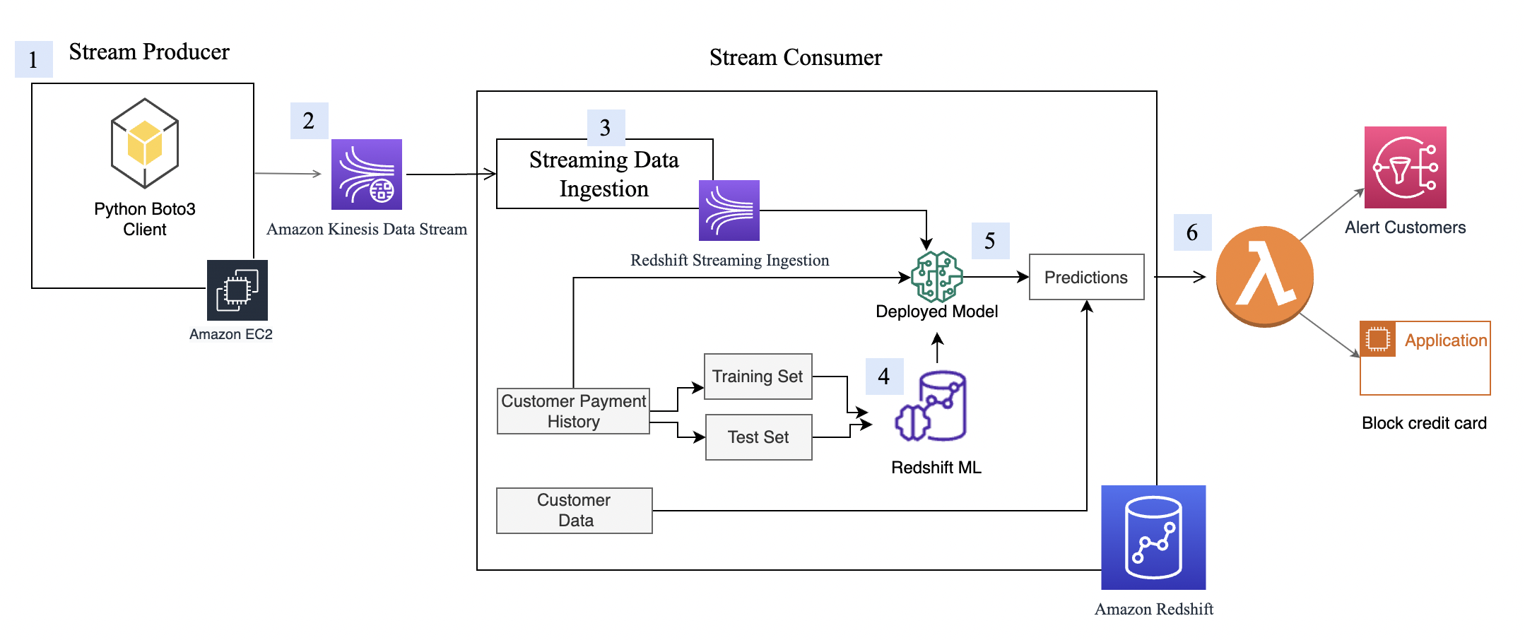
The step-by-step process is as follows:
- The EC2 instance simulates a credit card transaction application, which inserts credit card transactions into the Kinesis data stream.
- The data stream stores the incoming credit card transaction data.
- An Amazon Redshift Streaming Ingestion materialized view is created on top of the data stream, which automatically ingests streaming data into Amazon Redshift.
- You build, train, and deploy an ML model using Redshift ML. The Redshift ML model is trained using historical transactional data.
- You transform the streaming data and generate ML predictions.
- You can alert customers or update the application to mitigate risk.
This walkthrough uses credit card transaction streaming data. The credit card transaction data is fictitious and is based on a simulator. The customer dataset is also fictitious and is generated with some random data functions.
Prerequisites
- Create an Amazon Redshift cluster.
- Configure the cluster to use Redshift ML.
- Create an AWS Identity and Access Management (IAM) user.
- Update the IAM role attached to the Redshift cluster to include permissions to access the Kinesis data stream. For more information about the required policy, refer to Getting started with streaming ingestion.
- Create an m5.4xlarge EC2 instance. We tested Producer application with m5.4xlarge instance but you are free to use other instance type. When creating the instance, use the amzn2-ami-kernel-5.10-hvm-2.0.20220426.0-x86\_64-gp2 AMI.
- To make sure that Python3 is installed in the EC2 instance, run the following command to verity your Python version (note that the data extraction script only works on Python 3):
- Install the following dependent packages to run the simulator program:
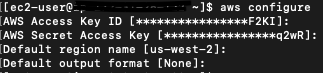
- Configure Amazon EC2 using the variables like AWS credentials generated for IAM user created in step 3 above. The following screenshot shows an example using aws configure.
Set up Kinesis Data Streams
Amazon Kinesis Data Streams is a massively scalable and durable real-time data streaming service. It can continuously capture gigabytes of data per second from hundreds of thousands of sources, such as website clickstreams, database event streams, financial transactions, social media feeds, IT logs, and location-tracking events. The data collected is available in milliseconds to enable real-time analytics use cases such as real-time dashboards, real-time anomaly detection, dynamic pricing, and more. We use Kinesis Data Streams because it’s a serverless solution that can scale based on usage.
Create a Kinesis data stream
First, you need to create a Kinesis data stream to receive the streaming data:
- On the Amazon Kinesis console, choose Data streams in the navigation pane.
- Choose Create data stream.
- For Data stream name, enter
cust-payment-txn-stream. - For Capacity mode, select On-demand.

- For the rest of the options, choose the default options and follow through the prompts to complete the setup.
- Capture the ARN for the created data stream to use in the next section when defining your IAM policy.

Set up permissions
For a streaming application to write to Kinesis Data Streams, the application needs to have access to Kinesis. You can use the following policy statement to grant the simulator process that you set up in next section access to the data stream. Use the ARN of the data stream that you saved in the previous step.
Configure the stream producer
Before we can consume streaming data in Amazon Redshift, we need a streaming data source that writes data to the Kinesis data stream. This post uses a custom-built data generator and the AWS SDK for Python (Boto3) to publish the data to the data stream. For setup instructions, refer to Producer Simulator. This simulator process publishes streaming data to the data stream created in the previous step (cust-payment-txn-stream).
Configure the stream consumer
This section talks about configuring the stream consumer (the Amazon Redshift streaming ingestion view).
Amazon Redshift Streaming Ingestion provides low-latency, high-speed ingestion of streaming data from Kinesis Data Streams into an Amazon Redshift materialized view. You can configure your Amazon Redshift cluster to enable streaming ingestion and create a materialized view with auto refresh, using SQL statements, as described in Creating materialized views in Amazon Redshift. The automatic materialized view refresh process will ingest streaming data at hundreds of megabytes of data per second from Kinesis Data Streams into Amazon Redshift. This results in fast access to external data that is quickly refreshed.
After creating the materialized view, you can access your data from the data stream using SQL and simplify your data pipelines by creating materialized views directly on top of the stream.
Complete the following steps to configure an Amazon Redshift streaming materialized view:
- On the IAM console, choose policies in the navigation pane.
- Choose Create policy.
- Create a new IAM policy called
KinesisStreamPolicy. For the streaming policy definition, see Getting started with streaming ingestion. - In the navigation pane, choose Roles.
- Choose Create role.
- Select AWS service and choose Redshift and Redshift customizable.
- Create a new role called
redshift-streaming-roleand attach the policyKinesisStreamPolicy. - Create an external schema to map to Kinesis Data Streams :
Now you can create a materialized view to consume the stream data. You can use the SUPER data type to store the payload as is, in JSON format, or use Amazon Redshift JSON functions to parse the JSON data into individual columns. For this post, we use the second method because the schema is well defined.
- Create the streaming ingestion materialized view
cust\_payment\_tx\_stream. By specifying AUTO REFRESH YES in the following code, you can enable automatic refresh of the streaming ingestion view, which saves time by avoiding building data pipelines:
Note that json\_extract\_path\_text has a length limitation of 64 KB. Also from\_varbye filters records larger than 65KB.
- Refresh the data.
The Amazon Redshift streaming materialized view is auto refreshed by Amazon Redshift for you. This way, you don’t need worry about data staleness. With materialized view auto refresh, data is automatically loaded into Amazon Redshift as it becomes available in the stream. If you choose to manually perform this operation, use the following command:
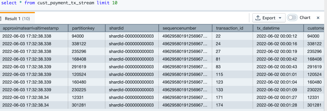
- Now let’s query the streaming materialized view to see sample data:
- Let’s check how many records are in the streaming view now:

Now you have finished setting up the Amazon Redshift streaming ingestion view, which is continuously updated with incoming credit card transaction data. In my setup, I see that around 67,000 records have been pulled into the streaming view at the time when I ran my select count query. This number could be different for you.
Redshift ML
With Redshift ML, you can bring a pre-trained ML model or build one natively. For more information, refer to Using machine learning in Amazon Redshift.
In this post, we train and build an ML model using a historical dataset. The data contains a tx\_fraud field that flags a historical transaction as fraudulent or not. We build a supervised ML model using Redshift Auto ML, which learns from this dataset and predicts incoming transactions when those are run through the prediction functions.
In the following sections, we show how to set up the historical dataset and customer data.
Load the historical dataset
The historical table has more fields than what the streaming data source has. These fields contain the customer’s most recent spend and terminal risk score, like number of fraudulent transactions computed by transforming streaming data. There are also categorical variables like weekend transactions or nighttime transactions.
To load the historical data, run the commands using the Amazon Redshift query editor.
Create the transaction history table with the following code. The DDL can also be found on GitHub.
Let’s check how many transactions are loaded:
Check the monthly fraud and non-fraud transactions trend:
Create and load customer data
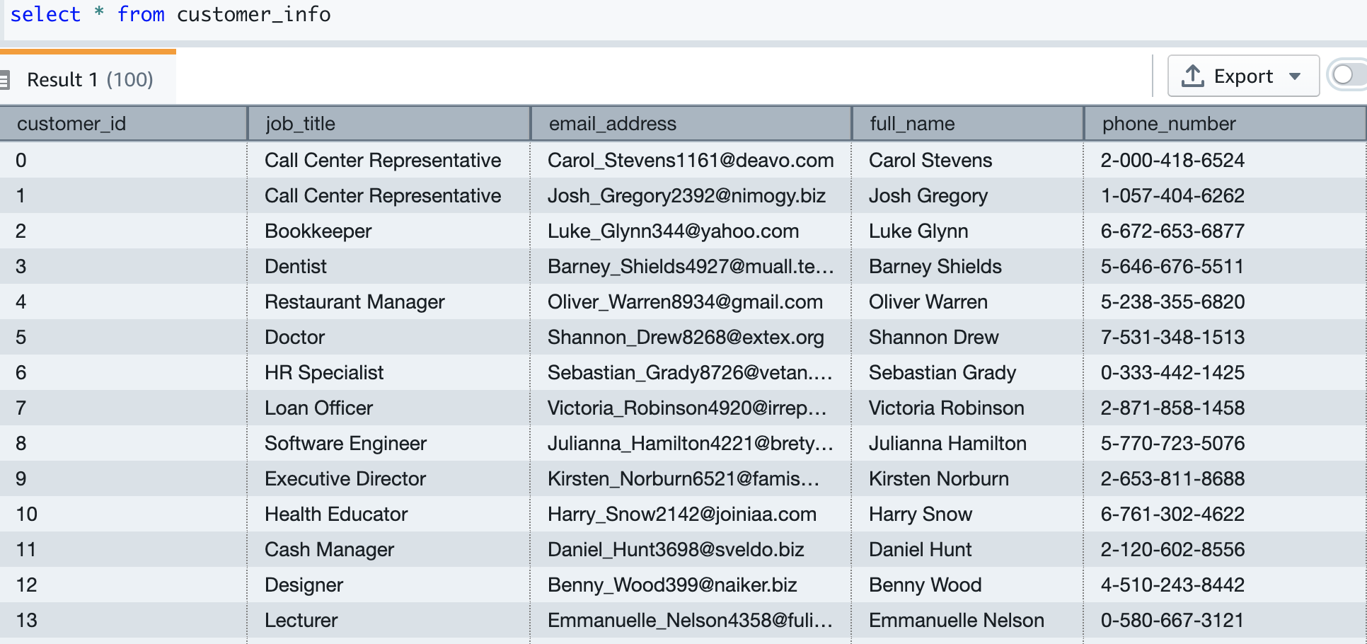
Now we create the customer table and load data, which contains the email and phone number of the customer. The following code creates the table, loads the data, and samples the table. The table DDL is available on GitHub.
Our test data has about 5,000 customers. The following screenshot shows sample customer data.
Build an ML model
Our historical card transaction table has 6 months of data, which we now use to train and test the ML model.
The model takes the following fields as input:
We get tx\_fraud as output.
We split this data into training and test datasets. Transactions from 2022-04-01 to 2022-07-31 are for the training set. Transactions from 2022-08-01 to 2022-09-30 are used for the test set.
Let’s create the ML model using the familiar SQL CREATE MODEL statement. We use a basic form of the Redshift ML command. The following method uses Amazon SageMaker Autopilot, which performs data preparation, feature engineering, model selection, and training automatically for you. Provide the name of your S3 bucket containing the code.
I call the ML model as Cust\_cc\_txn\_fd, and the prediction function as fn\_customer\_cc\_fd. The FROM clause shows the input columns from the historical table public.cust\_payment\_tx\_history. The target parameter is set to tx\_fraud, which is the target variable that we’re trying to predict. IAM\_Role is set to default because the cluster is configured with this role; if not, you have to provide your Amazon Redshift cluster IAM role ARN. I set the max\_runtime to 3,600 seconds, which is the time we give to SageMaker to complete the process. Redshift ML deploys the best model that is identified in this time frame.
Depending on the complexity of the model and the amount of data, it can take some time for the model to be available. If you find your model selection is not completing, increase the value for max\_runtime. You can set a max value of 9999.
The CREATE MODEL command is run asynchronously, which means it runs in the background. You can use the SHOW MODEL command to see the status of the model. When the status shows as Ready, it means the model is trained and deployed.
The following screenshots show our output.
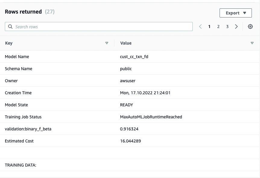
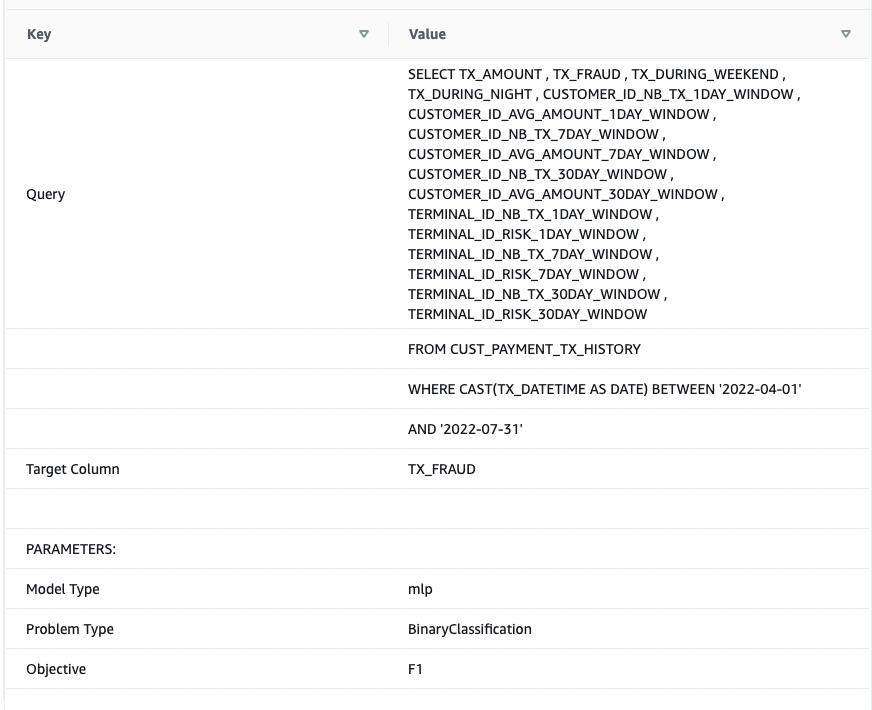
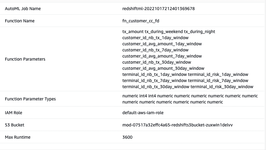
From the output, I see that the model has been correctly recognized as BinaryClassification, and F1 has been selected as the objective. The F1 score is a metric that considers both precision and recall. It returns a value between 1 (perfect precision and recall) and 0 (lowest possible score). In my case, it’s 0.91. The higher the value, the better the model performance.
Let’s test this model with the test dataset. Run the following command, which retrieves sample predictions:
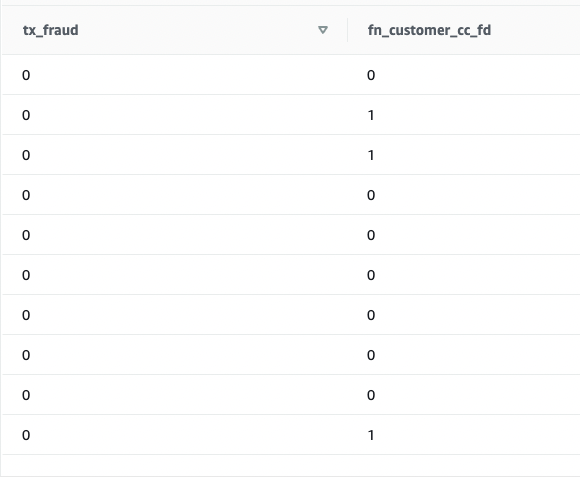
We see that some values are matching and some are not. Let’s compare predictions to the ground truth:
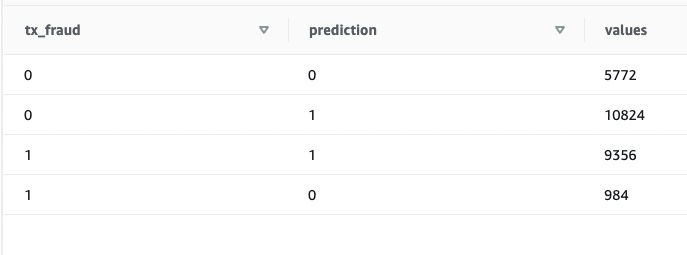
We validated that the model is working and the F1 score is good. Let’s move on to generating predictions on streaming data.
Predict fraudulent transactions
Because the Redshift ML model is ready to use, we can use it to run the predictions against streaming data ingestion. The historical dataset has more fields than what we have in the streaming data source, but they’re just recency and frequency metrics around the customer and terminal risk for a fraudulent transaction.
We can apply the transformations on top of the streaming data very easily by embedding the SQL inside the views. Create the first view, which aggregates streaming data at the customer level. Then create the second view, which aggregates streaming data at terminal level, and the third view, which combines incoming transactional data with customer and terminal aggregated data and calls the prediction function all in one place. The code for the third view is as follows:
Run a SELECT statement on the view:
As you run the SELECT statement repeatedly, the latest credit card transactions go through transformations and ML predictions in near-real time.
This demonstrates the power of Amazon Redshift—with easy-to-use SQL commands, you can transform streaming data by applying complex window functions and apply an ML model to predict fraudulent transactions all in one step, without building complex data pipelines or building and managing additional infrastructure.
Expand the solution
Because the data streams in and ML predictions are made in near-real time, you can build business processes for alerting your customer using Amazon Simple Notification Service (Amazon SNS), or you can lock the customer’s credit card account in an operational system.
This post doesn’t go into the details of these operations, but if you’re interested in learning more about building event-driven solutions using Amazon Redshift, refer to the following GitHub repository.
Clean up
To avoid incurring future charges, delete the resources that were created as part of this post.
Conclusion
In this post, we demonstrated how to set up a Kinesis data stream, configure a producer and publish data to streams, and then create an Amazon Redshift Streaming Ingestion view and query the data in Amazon Redshift. After the data was in the Amazon Redshift cluster, we demonstrated how to train an ML model and build a prediction function and apply it against the streaming data to generate predictions near-real time.
If you have any feedback or questions, please leave them in the comments.
About the Authors
 Bhanu Pittampally is an Analytics Specialist Solutions Architect based out of Dallas. He specializes in building analytic solutions. His background is in data warehouses—architecture, development, and administration. He has been in the data and analytics field for over 15 years.
 Praveen Kadipikonda is a Senior Analytics Specialist Solutions Architect at AWS based out of Dallas. He helps customers build efficient, performant, and scalable analytic solutions. He has worked with building databases and data warehouse solutions for over 15 years.
 Ritesh Kumar Sinha is an Analytics Specialist Solutions Architect based out of San Francisco. He has helped customers build scalable data warehousing and big data solutions for over 16 years. He loves to design and build efficient end-to-end solutions on AWS. In his spare time, he loves reading, walking, and doing yoga.